On Objectivity and Specificity of

the Probabilistic Basis for Testing.

By

G. Rasch.

1: Basic formula for the,simple dichotomic model.

One of the situations to be considered in the present paper is the following.

A number of elements, called "objects", characterized by positive scalar parameters, C1,•••,Cn , are exposed to a set of

other elements, called "agents", also characterized by positive

scalar parameters, c i ,... l ck . The "contact" between an object, no.. v , and an agent, no. i , produces with a certain probabili-

ty, depending upon C v and e i , one out of two possible responses,

called 1 and 0

Denoting the response by avi we then have

avi = 1 or 0 for v=1,...,n, i=1,...,k

For the set of nk responses we assume stochastic independence:

n k (1,2) 101((avi ))1(C v ),(Ei)/ = vill inl Pfavi l& v ,c i /

and for each pair (v,i) the probability is specified as

a ( v E i ) vi

(1.3) pfa v'e.1 = •1

This modal_ was presented in [2] and has been dealt with

elsewhere, but for easy reference we shall reproduce the basic steps in the algebraic theory of this "simple dichotomic model".-

According to (1.3) the probability (1.2) of any zero-one

matrix ((avi )) is

( 1 .4)

r s.

1-/ ne l

Pl((aviNg 1v

),( 6 .)} = (v) (i) Y(( v ),(E i ))

where T v and s i denote the marginal sums

E a . = r E a . = s. (i) vi v , (v)

1 ( 1 .5 )

and where for short

(1,6) II II (1+v1

E.) = Y(( v ),(cd. )) • (v) (i)

The further algebra may be simplified by using vector-matrix notations like

(1,7)

a** .((a. v)) l

= l'""n) ' E * = (El"'" Ek )

r* = (r 1"'"rn)23* = (sl'"" sk )

together with the following definition

a alk (1.8) x * = x1 ...x

of a real vector

x* = (x l ,...,xk )

raised to a power that is an enumerating vector

a (a 1 , ...,

each ai being an integer = 0 ,

and similarly for x** and a** being matrices. The convenience

of (1.8) lies partly in the condensation of the formulae and

partly in the obvious rule

x a,• x

The formula (1.4) takes on the form

r„ E

(1 .1 0) Pf a** * 7 *

a*+13 (1.9)

I (C*,E*)

P I T** y e* /

y(c* Ir* ) = r 7

(S ) ES;

pfs *

S * )1 ( IS ) 6*

6 1 - * i(c/6*)

Y( IS * ) = * 1 F (r ) [

With the symbol

(1.n ) S

*

for the number of zero-one matrices with the marginal vectors r and s it follows from (1.10) that

s*

(1.12)

plr* ,s* I * ,e * 1 = r* E*

-*' *

Summing over all vectors s that are compatible with a given

vector r * the marginal distribution

obtains, and on dividing that into (1.12) we get the conditional

distribution

(1.15) pfs * Ir*7 E* / = s* Y(E*Ir*)

Analogously

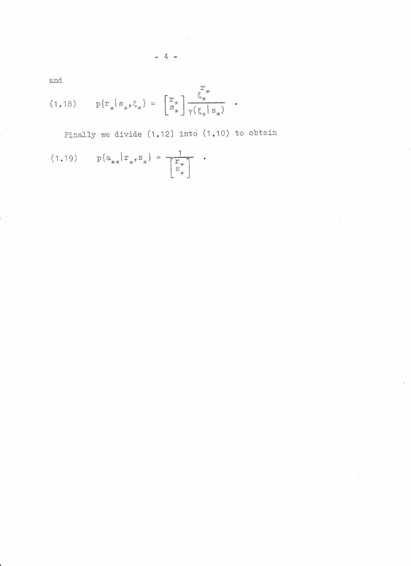
and

(1.18) pfr * Is**

r*

[rs *i y( Is)

Finally we divide (1.12) into (1.10) to obtain

( 1 .19) it I s = ** *

Comments upon appraisal of the parameters. - Specific objectivity.

2. The parameters 'C11 .„,Cn signify manifestations of a certain

property of a set of "objects" which are investigated by means

of a set of "agents" characterized by the parameters e il ...,Ek Thus in principle the C's stand for properties of the objects

per se, irrespective of which E i t S might be used for locating

them. Therefore they really ought to be appraised without any

reference to the Ei's actually employed for this purpose - just

like reading a. temperature of an object should give essentially

the same result whichever adequate thermometer were used.

Now the joint distribution (1.12) of r * and s* depends on

both sets of parameters. Therefore an evaluation of E„ 1 ,..., 11

based upon this probabilistic statement would in principle be

contaminated by the e i 's But the conditional distribution

(1.18) of r for given s is independent of e ; therefore an

evaluation of C based upon that statement will be unaffected

by which values the elements of E * may have. Of course, it

depends on s , the distribution of which,(1.16),in turn depends

on (and ) , but this is a different matter: s is a known

vector * is not and, in principle, never will become known.

The same argument of course applies to the e i 's , which by

means of (1.15) can be evaluated uninfluenced by the Vs

The separation of the parameters achieved by the formulae

(1.18) and (1,15) is closely related to the most fundamental

requirement in Natural Sciences, in particular in Physics,

namely that scientific statements should be objective*)

During centuries philosophers have disagreed about which

concept should be attached to the term objectivity, and on this

occasion I am not entering upon a discussion of that matter, I

only wish to point out that the above mentioned separation

exemplifies a type of objectivity which I qualify by the

predicate "specific". By which I mean that the statement in question - in the present case one about, say, the a-parameters

- is not affected by the free variation of contingent factors

within the specified frame of reference*

' ) , The frame of reference

cf. Hermann Weyl, Philosophy of Mathematics and Natural Science, Princeton University 1947, p. 71.

hero being the interaction of objects and agents, the agent

parameters are those which are contingent or incidental in state-

ments about the object parameters.

Now a statistician may ask: What is the price of this precious objectivity? DonTt we loose some valuable information

by insisting upon it?

In the present case the answer is: Not As a matter of fact,

the two conditional distributions (1.15) and (1.18) are equival-

ent with the joint distribution (1.12).

From the elementary formula

(2,1)

plr* ,s* IC * = Pfr Is 1P{s ems }

= T.) { ,s I r*lEJ-Pt r I F.,,E * 1

follows that

P{r IS 2* P{r fe (2.2) = E

(r u ) p{s ir (r* ) 13{s * } pls

which together with pfr.ls * , * 1 produces plr* ,s * I * , 6* / . That the expression thus obtained coincides with (1,12) is easily

verified,

To this may be added that when also (1.19) is taken into

account, the model itself, as expressed in (1.10), is com-

pletely recovered.

3, On the specificit- of a model control.

The formula (1.19) tells that the probability of the matrix

a conditional upon the marginal vectors r and s,, i2 in- ** dependent of all of the parameters, thus being a consequence

of the structure of the model,irrespective of the values of the

parameters, Therefore it would seem a. suitable basis for-a

specifically objective model control, i.e. for testing the

validity of the model in a way that is unaffected by the values

of the parameters Which as regards the structure of the model,

are the "contingent factors" within the given framework.

It should be noticed, however, that the derivation of (1.19)

only shows that if the model holds then this formula applies :

i.e. that (1.19) is a nescessar' condition for the model to •

hold. True enough, according to the preceding section we may,

taking (1.2) for granted, work back to (1,3), but only if (1.15)

and (1.18) are also taken into account.

The following statement concerns what can be concluded from

(1.19) without support from (1.15) and (1.18).

Theorem I. If the elements of a stochastic zero-one matrix

(3. 1) a **

= ((a V1 .)) v=1 ,oasey 9 i=1 , , ,., k yo,s,

are independent:

(3.2) pla*,1 (n) (

n )pla,.1 ,

vi

and if the distribution of the matrix, conditional upon the

marfnal vectors r x and s defined by (1.5) and (1.7) is

P. iven by (1.19) for a particular 'pair (r - s ) containing no uninformative elements - i,e, each r y / 0 and k , each s i / 0

and n - than two real, positive vectors

( 3 . 3 )

exist such that (1,3) holds for each air

vi vi Pf av ivi 1 = ----- • X > 0 vi 14Avi

a

(3.4)

Since all of the avi's are either 0 or 1 their probabilities

may be represented by

Due to the stochastic independence (3.2) the probability of

the matrix a becomes **

(3.5) p{ a **

a** **

* 1 = n n(1+x .y x** = (v) (i) vi

Summing over a** such that the marginal vectors are kept fixed

we get

(3.6) p(x ** Ir * ,s* )

p{,,,,s* Ix**} = (v) (i)

and in consequence

(3 .7)

whore

(3.8 )

p{a Ir I s ,X 1= ** * * **

a ** **

Y(X ir ,s ) ** * *

a Y(N. IT ,s =

x ** ** * *

with the same summation over a ** as above.

Now identification of (3.7) with (1.19) puts such restric-

tions on the X .'s that vi

a** p(X ir s ) (3.9)

** */ * **

must hold for all a es with the marginal vectors r and s **

Let

a** ..-((a

v .)) and a'** = ((alvi ))

be any two such matrices, then we must have

a at (3.10)

= *k **

or, taking logarithms,

(3.11) E E a.34, = E E at . ( v ) ( i) VI VI ( v)

(i) VI VI

where

(3.12). va. = log Xvi •

According to assumption no r y determines all of the elements

8.1)11 ....,avk ,neitherdoesanys.determine all of the elements

a1 i'"'' ani Therefore, marking any two object numbers,

p and v , and any two agent numbers, i and j it is possible •

to find two admissible matrices that are identical, except

where the rows no. p and v intersect the columns no. i and j ,

In those places we may have the elements

ma** in a' **

i j i j

(3.13) 1.t 1 0 p 0 1

v 0 1 v 1 0 .

Thus (3.11) requires that

(3.1 4 ) . = . . 111 vj PJ

for any two pairs (p., v) and (i 1 j), even for p=v and for i=j

since (3.14) then is trivial. Averaging now over p and j while v and i are kept fixed

we get

- 1 0 -

(3.14) 114. = V1 v . . • •

whichmeansthatX.factorizes into

(3. 1 5)

xi = vsi , v = V.

Si = e

On inserting this into (3.4) we get (1.3), which completes the

proof of the theorem ) .

With theorem I it becomes clear that, given the independence

(3.2), the relation (1.19) is a condition for the validity of

the model (1.3) which is both nescessary and sufficient. There-

fore I shall characterize (1.19) as El specific basis for testing

the structure - (1,3) of the model.

At the beginning of this section it was pointed out that

(1.19) is a specifically objective basis for the same testing.

These two concepts are fundamentally different.

From (1.19) some more special statements might be derived -

e.g. the conditional mean value of the product of all elements

of the matrix a** as a. function of r and s* • That would still

be objective since it is, of course, algebraically independent

of the parameters, but being 0 except for all r y = k (and all

s = n), the model cannot be deduced from this value alone.

And therefore it is not specific.

On the other hand, one might formulate a statement that is

specific, but involves all of the parameters - if nothing else,

then the relation (1.4) - and therefore not being objective.

In_ passing it may be noted that for the extension of (1.3) to

to independent binomial distributions

a .

.m ,E. va. v

1 = ( m . vi E.) Pfa

va.

a vi vi

which may sometimes be useful, both the basic algebra of sect.1

and the inversion theorem I generalize readily.

A probali,stic statement that combines the two properties,

specificity and specific objectivity, as we have it in (1.19),

would seem a most desirable point of departure for entering upon the testing of a hypothesis.

(4.1b)

then

(4.2) m 1 pf al a21 m 1 ,m2, 1 , C 2 1 =

Pla2 1 m221 = ( :2) c2

Mn 2 ( i+co )

a 2

- 12 -

4. On com arir two binotial distributions. Let a1 and a2 be stochastically independent and

(4-.1a)

a..

m1 \ Cl PI al = 1x1 1 '

For the sum

(4.3)

= a1 a2

the distribution is

Yo (C1'':2 1m1i m 2 ) plcim m r Cl= 2''1' 2 2 m m (1+C1 ) ) 1

with

(4.5) Yc (C1 C2 I ml ,m2 ) = E ( m2 ) C1al C2a2 al+are al a2

(

and furthermore

(4.6) Pl a1 a2 I c / m1 ' 111 2' Cl ' C2

11

)

cal ca2 a2 1 2

lc ( C1 C2 11:1 1 )

When

(4.7)

= c2=

- 1 3 -

- a hypothesis to be tested - this reduces to

(4.8)

and

(4.9)

Y e (C ,Clin 1 , m2 ) =

pfa 1 ,a2 1c,C l m 1

/ m 1 +m2 \ rc

(

al ) a2 )

M 4-M2) ( l c

which forms the basis for R, A. Fisher's "exact test" for

comparing two relative frequencies [1]

Clearly (4,9) is independent of the parameter C , which

according to the hypothesis is common to the two distributions

(4.1a) and (4.1b); thus it is specifically objective statement,

But furthermore it is specific for the hypothesis in

question: Theorem IIa, If the inde endent variables '1 and a2 follow

the binomial distributions (

) and if the conditional

distribution (4.6) is given by right hand term of (4.9),

then the two pframeters C i and must coincide. Theorem In. For the coincidence of C i and in (4,2) it

suffices that the distribution (4.6) is_21aLL21 .911v indepen-

dent of the ratio L;1L2_. To begin with the latter: As (4.5) is homogeneous in C i and

2 the right hand term of (4.6) depends only on their ratio. And if it is independent of that it must equal its value for

Ci = C, which according to (4.8) reduces to the right hand term of (4.9).

Identifying next the right hand terms of (4,6) and (4.9) we

find that

m l +m2 ̀"11 c2'2 Yc C2 1111 1 ' 111 2 ) = - 1 2

2 asholdingforallaand a. with the sum c . (4.7) follows ' from the identity for a 1 =c , a2.0 and a1.01a2=c

- 14 -

Low and again the adequacy of a test based solely upon (4,9)

has been questioned. Realizing, that this condition is both

necessary and sufficient for the hypothesis (4.7), provided

that we are at all dealing with independent binomially

distributed variables, I feel fully satisfied about the

adequacy of the basis for Fisher's test.

- 15 -

5. Generalizations. The results of the preceding section are readily generalized

to comparisons of several binomial distributions, of several

multinomial distributions, in fact to several "enumerative distributions", i.e. those of the form

as xa. ,

(5.1a) pla IX 1 = * a(X)

where a and X may be vectors:

(5.1b) pla a k X 1 = 1"'" '1"" , k

a ak a a1 1 • • • "k

a(X1'""

I may just indicate the steps in comparing two such

distributions. For (5 . 1 a) and b

Pb, • /4(. (5.2) plb* 14.1 *

(11* )

we have, independence being presumed, a. b

as pb • X *4 * - * * * * (5.3) pla 1 b IX*7 4 1 -

a (X* ) P(11* )

and

(5.4) Plc IX } - * * * a(X* ) P(I1* )

with

Ye (X4 ,11* )

c = a + b*

b, 11 ) = aa Pb , a b =c * * *

(5.6)

and

(5.7)

- 16 -

Accordingly

a b* af3 X 1.), a lb * *

p{a .b Ic I X 1 11A = ------ ------- (5.8) * *

is (Xla ) 9 *

which for

( 5.9)

X* =

becomes independent of the common parameter:

as pb * * p b c — 7 * re

-*

aa Pb Yc * a*+b*=c *

(5.10) then is a specifically objective statement, and it is a nescessary condition for (5.9). That it is also sufficient,

thus specific for (5.9), is seen by identifying (5.10) with

(5.8) which leads to

(5.12) a* b*

* Ye (X*' 11* ) = Ye X

as holding for any pair (a *l b* ) satisfying (5.6). It follows that

a -a k X ai (5.13) X *11 ** =

i=1

must remain constant under the passible variation of a * which is defined by

(5.14) 0 < a. c. = =

* * * *

1 0 x * p{x 16 } =• e * * 7177-7 a(x )

+Do 6..*x y(0 ) = f e *a(x.)dx I

k = II dx. .

i=1 1

- 17 -

Ifforan,yjwithci >

1wetakea..1 , all the other = J

a.i ls=0,itieseenthatX=Ili .Thus (5.9) must hold, except- ing elements with the corresponding c

j = 0 .

The properties demonstrated in some cases have, of course, to do with the Darmois-Koopman or Exponential family of •

distributions.

Without going into the general theory of this family I may

just indicate how the same train of thought works in the fol-

lowing very simple case of k-dimensional differentiable

distribution: With

( 5.1 5 )

we consider

1" k

*

For two distributions

6 x (5.18) 1 pfx le = v* 1 yOD

. v* via ( ) v=1,2 x v v* v*

of independent variables

x v* = (xv1'

xvk )

we have

a1 (x1* )a2 (x2* ) c 01* 1* e* x-,

(5.19) Pfx1* 2x2* 1 ei*$ 62.

-;= } .Y1 (61)72(62)

- 18 -

Transforming to xi* and

(5.20) Z* = X1*+X2*

we get

(5.21) p{x z 10 0 2#} 1*Y 1* , 2*

(x1* )a2 (z* -x13 ) e(el*

(6 1* ).Y2 (e 2* )

)x +e z 1* 2* *

and on integration with respect to xi*

(5.22) P {z* 1 e2* } — — Y1 (el *) i2 (62* )

+00 (0 -6 2 )t • f e

* *a 1 (t* )a°

0 z 2* *

-t* )dt *

On dividing this into (5.21) the conditional distribution of x1 , given z obtains:

(0-1- -62*/ x1* (x )a (z -x )e (5.23) p 1 z 0 - 1 1* 2 * 1* 1* 1* 1 1*/ 2* - +Do (0

1-62 it

f e Lt* /a2 (z* -t* )dt _co

which for

(5.24) 01* = 02* = 0*

simplifies to

- 1 9 -

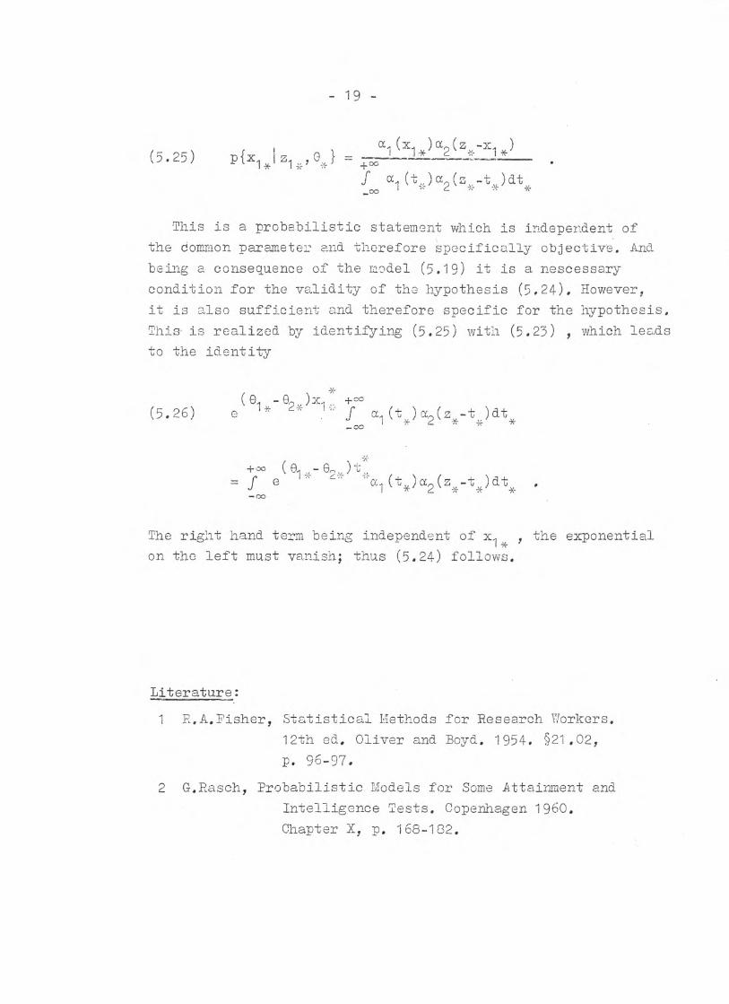
(5.25) Pbc1* lz1 , 0* 1 +00a 1 (x)a2 (z * -x1* )

f a1 (t * )a2 (z -t * )dt

This is a. probabilistic statement which is independent of the Common parameter and therefore Specifically objective. And

being a consequence of the model (5.19) it is a neseessary

condition for the validity of the hypothesis (5.24). However,

it is also sufficient and therefore specific for the hypothesis,

This is realized by identifying (5.25) with (5.23) which leads

to the identity

(5.26) (e1 , - e2* )dt * *

= f +°°

e(e1 - 24k )t 4 a ( t ie ) 0:2 (z *)dt -x-

The right hand term being independent of x l* , the exponential

on the left must vanish; thus (5.24) follows.

Literature:

1 R.A.Fisher, Statistical Methods for Research Workers.

12th ed. Oliver and Boyd. 1954. §21.02,

p. 96 - 97.

2 G.Rasch, Probabilistic Models for Some Attainment and

Intelligence Tests. Copenhagen 1960. Chapter X , p. 168-182.