ON-OFF THRESHOLD MODELS OF SOCIAL BEHAVIOR A Thesis Presented by Kameron Decker Harris to The Faculty of the Graduate College of The University of Vermont In Partial Fulfillment of the Requirements for the Degree of Master of Science Specializing in Mathematics October, 2012
Transcript
ON-OFF THRESHOLD MODELS OF
SOCIAL BEHAVIOR
A Thesis Presented
by
Kameron Decker Harris
to
The Faculty of the Graduate College
of
The University of Vermont
In Partial Fulfillment of the Requirementsfor the Degree of Master of Science
Specializing in Mathematics
October, 2012
Accepted by the Faculty of the Graduate College, The University of Vermont, in partial fulfillmentof the requirements for the degree of Master of Science, specializing in Mathematics.
Thesis Examination Committee:
AdvisorPeter Sheridan Dodds, Ph.D.
Christopher M. Danforth, Ph.D.
ChairpersonJoshua Bongard, Ph.D.
Dean, Graduate CollegeDomenico Grasso, Ph.D.
August 15, 2012
Abstract
We study binary state dynamics on a social network, where nodes act according to individualresponse functions of the average state of their neighborhood. These response functions modelthe competing tendencies of imitation and non-conformity by incorporating an “off-threshold” intostandard threshold models of behavior. In this way, we attempt to capture important aspects offashions and general societal trends.
Allowing varying amounts of stochasticity in both the network and response functions, we finddifferent outcomes in the random and deterministic versions of the model. In the limit of a large,dense network, however, these dynamics coincide. The dynamical behavior of the system rangesfrom steady state to chaotic depending on network connectivity and update synchronicity. A meanfield theory is laid out in detail for general random networks. In the undirected case, the mean fieldtheory predicts that the dynamics on the network are a smoothed version of the response functiondynamics. The theory is compared to simulations on Poisson random graphs with response functionsthat average to the chaotic tent map.
1 The four different ways the model can be realized. . . . . . . . . . . . . . . . . . . . 10
iii
List of Figures
1 A graph consisting of one isolated node and a connected component of 5 nodes. . . . 32 An example on-off threshold response function. . . . . . . . . . . . . . . . . . . . . . 103 The tent map stochastic response function, f(x), Eqn. (6.1). . . . . . . . . . . . . . . 184 Bifurcation diagram for the dense map Φ(φ;α), Eqn. (6.2). . . . . . . . . . . . . . . 195 Deterministic (FG-FR) dynamics on a small graph. . . . . . . . . . . . . . . . . . . . 226 The 3-dimensional bifurcation diagram computed from the mean field theory. . . . . 247 Mean field theory bifurcation diagram slices for various fixed values of z and α. . . . 258 Bifurcation diagram from fully stochastic (SG-SR) simulations. . . . . . . . . . . . . 25
iv
1 Introduction
Almost universally, people enjoy observing, speculating, and arguing about their fellow humans’
behavior, including what they are wearing, the music they listen to, and however else they might
express themselves. Trends fascinate, whether past, present, or future. Contemporary examples of
prevalent trends include skinny jeans, fixed-wheel bicycles, and products made by Apple Inc. In the
60’s, shag carpets and floral wallpaper would take their place. Trends are also prevalent in language:
“hipster” was popular in the 40’s and evolved into “hippie”, but it has been reappropriated today
with different connotations; “groovy” was once used seriously, and now comes out tongue-in-cheek.
The dynamics of these cultural phenomena are fascinating and complex. They reflect numerous
factors such as the political climate, social norms, technology, marketing, and history. These phe-
nomena are also influenced by events that are essentially random. We are usually able to explain
the emergence of a fad after the fact, but it is extremely difficult to predict a priori whether some
behavior will become popular. Furthermore, those behaviors which are adopted by a large fraction
of the population can lose their excitement and die out forever or later recur unpredictably.
In this work we describe a mathematical model of the rise and fall of trends. Our model is a
social contagion process, where people are influenced by the behavior of their friends. The agents in
the model act according to simple competing tendencies of imitation and non-conformity. One can
argue that these two ingredients are essential to all of the trends discussed in the first paragraph.
Simmel, in his classic essay “Fashion” (1957), believed that these are the essential forces behind the
creation and destruction of fashions.
The model is not meant to be quantitative, except perhaps in carefully designed experiments.
But it captures the features with which we are familiar: some trends take off and some do not; some
trends are stable while others vary wildly through time. Our model is closely related to the seminal
work of Granovetter (1978) and Schelling (1971). Being a mathematical model, it is also connected
to theories of percolation, disease spreading, and magnetism.
We focus on the derivation and analysis of dynamical master equations that describe the expected
evolution of the system state. Through these equations we are able to predict the behavior of the
social contagion process. In some cases, this can be done by hand, but most of the time we resort
to numerical methods for their iteration or solution.
This thesis is structured as follows. In Section 2, we introduce the reader to important back-
1
ground material relevant to the on-off threshold model. In Section 3, we define the model and its
deterministic and stochastic variants. In Section 4, we provide an analysis of the model when the
underlying network is fixed. Section 5 develops a mean field theory of the model in the most general
kind of random graphs. In Section 6, we consider the model on Poisson random graphs with a spe-
cific kind of response function. Our analysis is then applied to this specific case, and we compare the
results of simulations and theory. Finally, Section 7 presents conclusions and directions for further
research.
2 Background
2.1 Basics of graphs and networks
When modeling any dynamical system of many interacting particles or agents, we are often forced
to start with a simplified description of their interactions. In a solid, for example, atoms are situated
on some sort of lattice and assumed to interact only with their nearest neighbors. However, in many
cases the interactions we aim to model do not have the periodic structure of a lattice. Graphs,
which are just a set of points connected by lines, are a more general mathematical structure. We
denote a graph G as an ordered pair G = (V,E) where V is the set of vertices (also called nodes)
and E ⊆ V × V the set of edges (also called links). Here, E is a set of ordered pairs, and we denote
an edge from vertices a to b as ab ∈ E. The terms graph and network will be used interchangably,
but have acquired different connotations. Hackett (2011, §1.2.1) puts this rather nicely:
To model a complex system as a graph is to filter out the functional details of eachof its components, and the idiosyncrasies of their interactions with each other, and tofocus instead on the underlying structure (topology) as an inert mathematical construct.Although this technique is central also to network theory, the word network, in contrast,usually carries with it connotations of the context in which the overarching system exists,particularly when that system displays any sort of nonlinear dynamics. For example,when investigating the spread of infectious disease on a human sexual contact networkit makes sense to consider the relevant sociological parameters as well as the abstracttopology, and it is in such settings that the interdisciplinary aspect that distinguishesnetwork theory comes to the fore.
In models of human behavior, interactions can be considered to occur on a social network. Each
person is connected to those people they interact with. Interactions that constitute a connection
between two people, A and B, may be defined in many ways. For example:
1. A contacts B. This could mean:
2
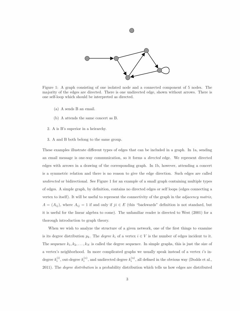
Figure 1: A graph consisting of one isolated node and a connected component of 5 nodes. Themajority of the edges are directed. There is one undirected edge, shown without arrows. There isone self-loop which should be interpreted as directed.
(a) A sends B an email.
(b) A attends the same concert as B.
2. A is B’s superior in a heirarchy.
3. A and B both belong to the same group.
These examples illustrate different types of edges that can be included in a graph. In 1a, sending
an email message is one-way communication, so it forms a directed edge. We represent directed
edges with arrows in a drawing of the corresponding graph. In 1b, however, attending a concert
is a symmetric relation and there is no reason to give the edge direction. Such edges are called
undirected or bidirectional. See Figure 1 for an example of a small graph containing multiple types
of edges. A simple graph, by definition, contains no directed edges or self loops (edges connecting a
vertex to itself). It will be useful to represent the connectivity of the graph in the adjacency matrix,
A = (Aij), where Aij = 1 if and only if ji ∈ E (this “backwards” definition is not standard, but
it is useful for the linear algebra to come). The unfamiliar reader is directed to West (2001) for a
thorough introduction to graph theory.
When we wish to analyze the structure of a given network, one of the first things to examine
is its degree distribution pk. The degree ki of a vertex i ∈ V is the number of edges incident to it.
The sequence k1, k2, . . . , kN is called the degree sequence. In simple graphs, this is just the size of
a vertex’s neighborhood. In more complicated graphs we usually speak instead of a vertex i’s in-
degree k(i)i , out-degree k(o)i , and undirected degree k(u)i , all defined in the obvious way (Dodds et al.,
2011). The degree distribution is a probability distribution which tells us how edges are distributed
3
among nodes. The average degree z =∑∞
i=0 kpk characterizes the overall density of edges. A degree
distribution which is sharply peaked about its mean indicates a relatively homogeneous network
where vertices tend to have the same number of incident edges. In contrast, a skewed distrbution
could result in some nodes having very high degree while the majority have low degree. This is
common in real networks, and the tail of the degree distribution often follows an approximate power
law pk ∼ k−α for some exponent α (Newman, 2003).
2.2 Random graphs
Random graphs are a family of models used to represent networks from the real world, although
their suitability as such is questionable for reasons that will be elaborated below. Nevertheless, they
are well-suited to analysis and as null models.
The simplest random graph is the binomial model introduced by Erdos and Renyi (Bollobas,
2001). Define a probability space G(N, p) of graphs on N vertices where any of the(N2
)
possible
edges are chosen independently with probability p. The average degree in the network will be
z = p(N − 1). We will often make statements about this network in the limit of large system size
N → ∞. (In physics, this is referred to as the thermodynamic limit. Many expressions are simplified
in performing this approximation, and derived results can be quite accurate given a large enough,
albeit finite, N .) The degree distribution pk ≡ P (K = k) =(N−1
k
)
pk(1 − p)N−1−k, a binomial
distribution, is well approximated by the Poisson distribution pk = zke−z/k! with parameter z = Np
when N is large and z fixed. For this reason, G(N, p) is also called the Poisson random graph model.
As noted previously, many networks observed in the real world have heavy-tailed distributions, so
the Poisson model is not suitable for those types of networks. Furthermore, real networks often
contain a high density of triangles or clustering — friendship tends to be transitive. Poisson random
graphs, on the other hand, have zero clustering in the thermodynamic limit.
A more flexible generalization is the configuration model. In this model, either the degree
sequence (Molloy and Reed, 1995, 1998) or the expected degree sequence (Chung and Lu, 2002)
is given in advance (also see Newman, 2003); the models produce similar networks with subtle
differences. The configuration model of Molloy and Reed (1995, they were not the first to consider
it; see the references therein) can be thought of as a random wiring process as follows. First, draw a
degree sequence k1, . . . , kN independently according to the desired degree distribution pk. We assign
ki stubs (half-edges) to each vertex i ∈ V . Next, choose a pair of stubs at random, connect them,
4
remove both from the queue of stubs, and continue until all stubs are connected. The resulting graph
will have the imposed degree sequence, so long as the sum of the degrees is even. There may be self-
loops or repeated edges, neither of which are allowable for simple graphs. However, we expect these
to occur increasingly rarely for large N , and they can be removed without affecting the resulting
graph much. Degree-degree correlations can be introduced by shuffling edges as described in Melnik
et al. (2011) and Payne et al. (2011). The configuration model also lacks triangles and higher-order
cliques in the thermodynamic limit, although some work has been done to create random graph
models with clustering (see Hackett, 2011, §§4-5).
2.3 Dynamical processes on networks
Networks provide a topology on top of which all kinds of dynamical processes take place. In many
cases, the structure of the network itself heavily influences the dynamics. For instance, ferromagnetic
materials can be modeled as atoms in a lattice network, where the bulk magnetization is the result
of interactions between individual atoms’ magnetic moments; strikingly different results occur in
different dimensional lattices. Another example is a food web, a network of species connected by
trophic interactions (being eaten or eating someone else). The populations of the species in the
ecosystem can be described by dynamical equations that reflect the structure of the network, and
this can affect ecosystem stability. These are just two examples where dynamical processes on
networks are a reasonable way to model system behavior. Since networks are ubiquitous structures,
these models appear across all disciplines (Vespignani, 2012).
2.3.1 Random boolean networks
Consider boolean or binary state dynamics, where each node can be either “on” or “off” (in various
contexts this can mean active/inactive, infected/susceptible, or spin up/spin down). The state of
node i is encoded by a variable xi ∈ 0, 1, and the system state is x = (xi). At each time step,
nodes receive input from their neighbors in the graph. They then compute a function of that input,
i.e. fi(xj1 , xj2 , . . . , xjki) where j1, . . . , jki
are the neighbors of node i. This determines their state in
the next time step. Because the state space 0, 1N is finite, all trajectories are eventually periodic.
The detailed structure of the cycles depends “combinatorially” on the details of the network and
the boolean functions.
The dynamics described above, for general fi : 0, 1ki → 0, 1, are known as a boolean net-
5
works. These were first studied by Kauffman (1969) as a model for dynamical behavior within cells.
See the review by Aldana et al. (2003). Most researchers have considered the dynamics on random
K-regular graphs with a parameter p that determines the bias between 0s and 1s in the output of
the update functions fi, which are otherwise randomly chosen boolean functions.
As mentioned, deterministic boolean network models must be eventually periodic. However, the
behavior of the transient and the structure of the basins of attraction are different for different
parameters K and p. In particular, there is a critical value of the connectivity Kc(p) that separates
the transient dynamics into two phases (Aldana et al., 2003):
1. Frozen, K < Kc: The distance between nearby trajectories x(t) and x′(t) decays exponentially
with time.
2. Critical, K = Kc: The temporal evolution of distance between trajectories is determined by
fluctuations.
3. Chaotic, K > Kc: The distance between nearby trajectories grows exponentially with time.
Note that in the rest of this thesis, p will always refer to the probability of connection in the
G(N, p) Poisson random graph model, and K will always refer to the random variable for node
degree.
2.3.2 Social models
When modeling social systems with a boolean network, the nodes represent people and their states
encode whether or not they participate in a behavior, possess a certain belief, etc. This could be
rioting or not rioting (Granovetter, 1978), buying a particular style of tie (Granovetter and Soong,
1986), liking a particular band or style of music, or believing in some controversial or unintuitive
idea, e.g. climate change. The state can represent any behavior with only two mutually exclusive
possibilities.
The function fi that determines how node i changes state is called its response function in
sociological contexts. Granovetter (1978) and Schelling (1971, 1973) pioneered the use of threshold
response functions in models of collective social behavior (although they were not the first; see the
citations in their papers). This was based on the intuition that, in order for a person to adopt some
new behavior, the fraction of the population exhibiting that behavior might need to exceed some
6
critical value, the person’s threshold. These models were generalized to the case where the dynamics
take place on a network by Watts (2002). If we initialize a social network with some fraction of active
nodes, some of their neighbors’ thresholds may be exceeded and the activity can spread (depending
on the distribution of thresholds and network structure). A threshold response function f(x; r) with
threshold r returns 0 if x < r and 1 if x ≥ r. The edge case could be defined differently, but this
will not influence the dynamics except in carefully constructed “pathological” scenarios.
Standard threshold models have simple dynamical behavior: in a word, “spreading”. If a single
activation, on average, leads to more than one subsequent activation, then the spreading will be
successful. The activity will increase in a sigmoidal fashion until some final fraction of the network
is activated. These kinds of spreading are often studied with branching processes. See the excellent
book by Harris (1963) for an overview of branching processes and the widely-used generating function
formalism. Branching processes have been used to model, among other things, extinction of families,
species, and genes, neutron cascades (as happens during nuclear chain reactions), and high energy
particle showers caused by cosmic rays. The generating function formalism developed in part by
Newman (as in Newman, 2003; Watts, 2002) to analyze spreading on networks is a straightforward
application of the classical theory of branching processes.
There have been papers in the literature concerning threshold random boolean network models
for modeling neural networks (Aldana et al., 2003). Those models take place on signed, weighted
graphs, which differ from the networks considered here, and the problems considered are different.
It would be interesting to explore the connections between our on-off threshold model (Section 3)
and other threshold boolean network models.
2.4 Some notation
The Bachmann-Landau asymptotic notations are used throughout this thesis. When used carefully,
asymptotic notation greatly improves the readability of analytic statements and proofs. It is also
widely used in probability. For an overview of the notation’s history and usage, see Knuth (1976)
and the references therin. The notations we have used here are (citing from Knuth (1976)):
• O(f(n)) is the set of all g(n) such that there exist positive constants C and n0 with |g(n)| ≤
Cf(n) for all n ≥ n0.
• Ω(f(n)) is the set of all g(n) such that there exist positive constants C and n0 with g(n) ≥
7
Cf(n) for all n ≥ n0.
• o(f(n)) is the set of all g(n) such that g(n)/f(n) → 0 as n → ∞.
• g(n) ∼ f(n) if g(n)/f(n) → 1 as n → ∞.
Formally, each of the above define sets of functions, but we often statements such as “f is O(g)”
(often read “f is big-oh of g”) to mean “f ∈ O(g)”.
When expressing probabilities we will use notation of the form P (X = x), P (X = x|Y = y),
etc. Here, P (X = x) is the probability that random variable X equals the value x. Upper-case
characters will generally correspond to the random variable, while lower-case characters correspond
to the value of the variable.
Symbols in boldface, e.g. x, represent vector quantities or vector-valued functions.
3 The on-off threshold model
Let G = (V,E) be a graph with N = |V |. Assign each vertex i ∈ V an on-threshold ri and an off-
threshold si, with 0 ≤ ri ≤ si ≤ 1. Then that node’s response function fi(x; ri, si) is 1 if ri ≤ x ≤ si
and 0 otherwise. Let x(0) ∈ 0, 1N be the initial states of all nodes. At time step t, every node i
computes the fraction φi of their neighbors in G who are active and takes the state fi(φi; ri, si) at
the next time step t+ 1.
The above defines a deterministic model for a fixed graph with fixed response functions. It is
thus a type of boolean network (Section 2.3.1). In the rest of this Section, we will describe how
this model is different from the random boolean networks in the literature. This is mainly due to
the on-off threshold response functions we consider, but also the type of random graph on which
the dynamics take place, varying amounts of stochasticity which we introduce in the networks and
response functions, and possibly asynchronous updates.
Here we study a simple extension of the classical threshold models (such as Granovetter, 1978;
Schelling, 1971, 1973; Watts, 2002; Dodds and Watts, 2004, among others): the response function
also includes an off-threshold. See Figure 2 for an example. This is exactly the model of Granovet-
ter and Soong (1986), but on a network. We motivate this choice of response functions with the
8
following (also see Granovetter and Soong, 1986). (1) Imitation: the on state becomes favored as
the fraction of active neighbors surpasses the on-threshold (bandwagon effect). (2) Non-conformity:
the on state is eventually less favorable with the fraction of active neighbors past the off-threshold
(reverse bandwagon, snob effect). (3) Simplicity: in the absence of any raw data of “actual” re-
sponse functions, which are surely highly context-dependent and variable, we choose the simplest
deterministic functions which capture imitation and non-conformity.
Repeating ourselves somewhat, note that a node activates if and only if its input is within a given
range, otherwise it deactivates. Each node is assigned an on-threshold r and an off-threshold s which
must satisfy 0 ≤ r ≤ s ≤ 1. The response function f(x; r, s) is 1 if r ≤ x ≤ s and 0 otherwise. Each
node reacts only to the fraction of its neighbors who are active, rather than the absolute number.
The input varies from 0 to 1 in steps of 1/k, where k is the node’s degree. Note that if r = 0 the
node activates spontaneously, and if s = 1 we have the usual kind of threshold response function
(with no off-threshold).
A crucial difference between our model and many related threshold models is that, in those
models, an activated node can never reenter the susceptible state. Gleeson and Cahalane (2007)
call this the permanently active property and elaborate on its importance to their analysis. Such
models must eventually reach a steady state. When the dynamics are deterministic, this will be
a fixed point, and in the presence of stochasticity the steady state is characterized by some fixed
fraction of active nodes subject to fluctuations. The introduction of the off-threshold builds in a
mechanism for node deactivation. Because nodes can now recurrently transition between on and off
states, the long time behavior of the deterministic dynamics can be periodic, with potentially high
period. With stochasticity, the dynamics can be chaotic.
3.2 The networks considered
The mean field analysis in Section 5 is applicable to any network characterizable by its degree
distribution. As mentioned before, the vast majority of the theory of random boolean networks
assumes a regular random graph. Fortunately, such theories are easily generalized to other types
of graphs with independent edges, such as Poisson and configuration model random graphs. Some
specific results are given for G a realization of the Poisson random graph G(N, z/N), and these are
the networks considered in Section 6.
9
0 r 0.5 s 10
0.2
0.4
0.6
0.8
1
xf(x
)
Figure 2: An example on-off threshold response function. Here, r = 0.33 and s = 0.85. The nodewill activate if r ≤ x ≤ s, where x is the fraction of its neighbors who are active. Otherwise it turnsoff.
Table 1: The four different ways the model can be realized. These are the combinations of fixedor stochastic graphs and response functions. In the thermodynamic limit of the totally stochasticversion, where the graph and response functions change every time step, the mean field theory(Section 5) is exact.
3.3 Stochastic variants
The specific graph G and node thresholds ri, si determine exactly which behaviors are possible. These
are chosen from some distribution of graphs, such as G(N, z/N), and distribution of thresholds with
joint density P (R = r, S = s). The specific graph and thresholds define a realization of the model
(see Aldana et al., 2003). When these are fixed for all time, then we have full knowledge of the
possible model dynamics. Given an initial condition x(0), the dynamics x(t) are deterministic and
known for all t ≥ 0.
With the introduction of noise, the system is no longer eventually periodic. Fluctuations at the
node level allow a greater exploration of state space, and the behavior is comparable to that of the
general class of discrete-time maps. Roughly speaking, the mean field theory we develop in Section
5 becomes more accurate as more stochasticity is introduced.
We allow randomness to be introduced to the network and/or response functions of the model.
Taking all of their possible combinations yields four different, yet similar, designs (see Table 1).
10
3.3.1 Stochastic graphs
First, the network itself can change every time step. This is the stochastic, as opposed to fixed,
network version of the model. For example, we could draw a new graph from G(N, z/N) every
time step. This amounts to rewiring the links while keeping the degree distribution fixed, and is
alternately known as a mean field or random mixing variant of the deterministic model. Statistical
physicists also use the words “annealed” (for stochastic) and “quenched” (for fixed) (see Aldana
et al., 2003, for an explanation and a short history of the terms).
3.3.2 Stochastic responses
Second, the response functions can change every time step. This is the stochastic response function
version of the model. Again, we will need a well-defined distribution P (R = r, S = s) for the
thresholds. For large N this amounts to a single response function f , the expected response function
f(x) =
∫
da
∫
db P (R = r, S = s)f(x; r, s). (3.1)
We call f : [0, 1] → [0, 1] the stochastic response function. Its interpretation is the following. For an
updating node with a fraction x of active neighbors at the current time step, then, at the next time
step, the node assumes the state 1 with probability f(x) and the state 0 with probability 1− f(x).
3.3.3 The concept of “temperature” in the system
In this thesis, the network and response functions are either fixed for all time or are resampled every
time step. One could tune smoothly between the two extremes by introducing rates at which these
reconfigurations occur. These rates are inversely related to quantities that behave like temperature
(one for the network and another for response funcitions). When in the fixed case, the temperature
is zero, and there are no fluctuations. In the stochastic case, the temperature is very large or infinite,
and fluctuations occur every time step.
3.4 Synchronicity of the update
Finally, we introduce a parameter α for the probability that a given node updates. When α = 1,
all nodes update every time step, and the update rule is said to be synchronous. When α = 1/N ,
only one node is expected to update with each timestep, and the update rule is said to be totally
11
asynchronous. This is equivalent to a randomly ordered serial update. For intermediate values, α is
the expected fraction of nodes which update each time step.
4 Fixed networks
Take the case where the response functions and graph are fixed (FG-FR), but the update may be
synchronous or asynchronous. Let xi(t) be the probability that node i is in state 1 at time t. The
dynamics follow the master equation
xi(t+ 1) = αfi
(
∑Nj=0 Aijxj(t)∑N
j=0 Aij
)
+ (1− α)xi(t), (4.1)
which can be written in matrix-vector notation as
x(t+ 1) = αf (Tx(t)) + (1− α)x(t). (4.2)
Here T = D−1A is sometimes called the transition probability matrix (in the context of a random
walker), D is the diagonal degree matrix, and f = (fi). Eqns. (4.1) and (4.2) are not entirely correct
when there are isolated nodes. In that case, ki =∑
j Aij = 0 for certain i, thus the denominator in
(4.1) is zero and D−1 undefined. If the initial network contains isolated nodes, set all entries in the
corresponding rows of T to zero.
The matrix L = D−A is called the Laplacian (sometimes the combinatorial Laplacian) and L =
I −D−1/2AD−1/2 is called the normalized Laplacian (I is the identity). So T = D−1/2(I −L)D1/2.
We see that T is similar to I −L, and the associated change of basis is a rescaling of axis i by√ki.
4.1 Asynchronous limit
Here, we show that when α ≈ 1/N , time is effectively continuous and the dynamics can be described
by an ordinary differential equation. This is similar to the analysis of Gleeson (2008). Consider Eqn.
4.2. Subtracting x(t) from both sides and setting ∆x(t) = x(t+ 1)− x(t) and ∆t = 1 yields
∆x(t)
∆t= α (f(Tx(t))− x(t)) . (4.3)
12
Since α is assumed small, the right hand side is small, and thus ∆x(t) is also small. Making the
continuum approximation dx(t)/dt ≈ ∆x(t)/∆t yields the differential equation
dx
dt= α (f(Tx)− x) . (4.4)
The parameter α sets the time scale for the system. Similar asynchronous, continuous time limits
apply to the dynamical equations in the dense case, Eqn. (4.5), and in the mean field theory, Eqns.
(5.3) and (5.4).
4.2 Dense network limit for Poisson random graphs
The following result is particular to Poisson random graphs, but similar results are possible for
other random graphs with dense limits. By Oliveira (2010), when z is Ω(logN) there exists a typical
Laplacian matrix Ltyp = IN − 1N1†N/N such that the actual L ≈ Ltyp in the induced 2-norm
(spectral norm) with high probability. We let 1N denote the length-N vector of ones and (·)† the
matrix transpose. In this limit, T ≈ T typ = 1N1†N/N . So T effectively averages the node states:
Tx(t) ≈ T typx(t) =∑N
i=1 xi(t)/N ≡ φ(t). We make this approximation in Eqn. 4.2 and average
Note that the edge-oriented state variable ρ contains all of the dynamically important information,
rather than the vertex-oriented variable φ.
5.2 Analysis of the map equation
The function Fk(ρ; f) is known in polynomial approximation theory as the kth Bernstein polynomial
(in the variable ρ) of f (Phillips, 2003; Pena, 1999). These are approximating polynomials which
have applications in computer graphics due to their “shape-preserving properties”. The Bernstein
operator Bk takes f -→ Fk. This is a linear, positive operator which preserves convexity for all k
and exactly interpolates the endpoints f(0) and f(1). Immediate consequences include that, for
concave f (e.g. the tent map or logistic map), we have concave Fk for all k and Fk ↑ f uniformly.
This convergence is typically slow. Importantly, Fk ↑ f implies that g(ρ; pk, f) < f for any degree
distribution pk. Also, each Fk is a smooth function and the derivatives F (k)k (x) → f (k)(x) where
f (k)(x) exists.
In some cases, the dynamics of the undirected mean field theory given by ρ(t + 1) = G(ρ(t)),
Eqn. (5.3), are effectively those of the map Φ, from the dense limit Eqn. (4.5). This is hinted at by
the shape-preserving properties of Bernstein polynomials. Let qk = kpk/z; this is sometimes called
the edge-degree distribution, since it represents the probability that a random stub is connected to a
degree k vertex. We see that g(ρ; pk, f), Eqn. (5.2), can be seen as the expectation of a sequence of
random functions Fk under the edge-degree distribution (indeed, this is how it was derived). From
the convergence of the Fk’s, we expect g(ρ; pk, f) ≈ f(ρ) if z is “large enough” and the edge-degree
distribution has a “sharp enough” peak about z. Then as z → ∞ the mean field coincides with the
15
dense network limit we found for Poisson random graphs, Eqn. 4.5. Some thought leads to a sufficient
condition for this kind of convergence: the standard deviation σ(z) of the degree distribution must be
o(z). In Appendix A we prove this as Lemma 1. If the original degree distribution pk is characterized
by having mean z, variance σ2, and skewness γ1, then the edge-degree distribution qk will have mean
z+σ2/z and variance σ2[1+ γ1σ/z− (σ/z)2]. Considering the behavior as z → ∞, we can conclude
that requiring σ ∈ o(z) and γ1 ∈ o(1) are sufficient conditions on pk to apply Lemma 1. Poisson
degree distributions (σ =√z and γ1 = z−1/2) fit these criteria.
5.3 Generalized random networks
In the most general kind of random networks, edges can be undirected or directed. In that case node
degree is denoted by a vector k = (ku, ki, ko)†. The degree distribution is written as pk ≡ P (K = k).
There may also be correlations between node degrees. Correlations of this type are encoded by
the conditional probabilities p(u)k,k′ ≡ P (K = k, u|K′ = k′), p(i)
k,k′ ≡ P (K = k, i|K′ = k′), and
p(o)k,k′ ≡ P (K = k, o|K′ = k′), the probability that an edge starting at a degree k′ node ends at
a degree k node and is, respectively, undirected, incoming, or outgoing relative to the destination
degree k node. We introduced this convention in (Payne et al., 2011). These conditional probabilities
can also be defined in terms of the joint distributions of node types connected by undirected and
directed edges.
The mean field equations for the on-off threshold model are closely related to the equations for
the time evolution of a contagion process (Payne et al., 2011, Eqns. (13–15)). We omit a detailed
derivation, since it is similar to that in Section 5.1 (see also Payne et al., 2011; Gleeson and Cahalane,
2007). The result is a coupled system of equations for the density of active stubs which now may
16
depend on node type (k) and edge type (undirected or directed):
ρ(u)k
(t+ 1) =α∑
k′
p(u)k,k′
k′
u∑
ju=0
k′
i∑
ji=0
(
k′uju
)(
k′iji
)
×[
ρ(u)k′ (t)
]ju [
1− ρ(u)k′ (t)
](k′
u−ju)
×[
ρ(i)k′ (t)
]ji [
1− ρ(i)k′ (t)
](k′
i−ji)
f
(
ju + jik′u + k′i
)
+ (1− α)ρ(u)k
(t) (5.6)
ρ(i)k(t+ 1) =α
∑
k′
p(i)k,k′
k′
u∑
ju=0
k′
i∑
ji=0
(
k′uju
)(
k′iji
)
×[
ρ(u)k′ (t)
]ju [
1− ρ(u)k′ (t)
](k′
u−ju)
×[
ρ(i)k′ (t)
]ji [
1− ρ(i)k′ (t)
](k′
i−ji)
f
(
ju + jik′u + k′i
)
+ (1− α)ρ(i)k(t) . (5.7)
The active fraction of nodes at a given time is given by:
φ(t+ 1) =α∑
k
pk
ku∑
ju=0
ki∑
ji=0
(
kuju
)(
kiji
)
×[
ρ(u)k
(t)]ju [
1− ρ(u)k
(t)](ku−ju)
×[
ρ(i)k(t)]ji [
1− ρ(i)k(t)](ki−ji)
f
(
ju + jiku + ki
)
+ (1− α)φ(t) . (5.8)
6 Poisson random graphs with tent map average response
function
The results so far have been entirely general, in the sense that the underlying network and thresholds
are arbitrary. Now we apply the general theory to the case of Poisson random graphs with a simple
distribution of thresholds.
The networks we consider are Poisson random graphs from G(N, z/N). The thresholds r and
s are distributed uniformly on [0, 1/2) and [1/2, 1), respectively. This distribution results in the
17
0 0.2 0.4 0.6 0.8 10
0.2
0.4
0.6
0.8
1
x
f(x)
z=1 10 100
Figure 3: The tent map stochastic response function, f(x), Eqn. (6.1). Also shown are the edgemaps g(x; z) = g(x; pk, f), Eqn. (5.2), for z = 1, 10, 100. These pk are Poisson distributions withmean z, and f is the tent map. As z increases, g(x; z) approaches f .
stochastic response function
f(x) =
2x : 0 ≤ x < 1/2
2− 2x : 1/2 ≤ x ≤ 1, (6.1)
shown in Figure 3. The tent map is a well-known chaotic map of the unit interval (Alligood et al.,
1996). We thus expect the on-off threshold model with this stochastic response function to exhibit
similarly interesting behavior.
6.1 Analysis of the dense limit
When the network is in the dense limit (Section 4.2), the dynamics follow φ(t + 1) = Φ(φ(t);α),
where
Φ(φ;α) = αf(φ) + (1− α)φ =
(1 + α)φ : 0 ≤ φ < 1/2
(1− 3α)φ+ 2α : 1/2 ≤ φ ≤ 1. (6.2)
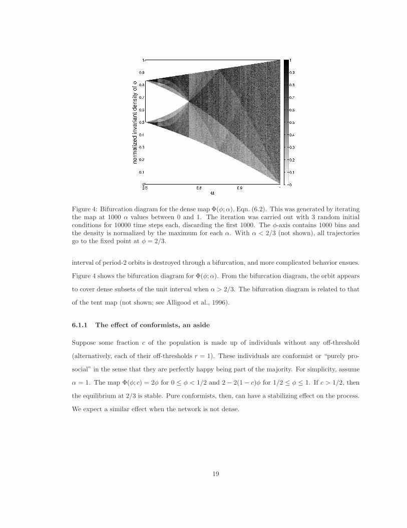
Solving for the fixed points of Φ(φ;α), we find one at φ = 0 and another at φ = 2/3. When α < 2/3,
the nonzero fixed point is stable. When α = 2/3, [1/2, 5/6] is an interval of period-2 orbits. Any
orbit will eventually land on one of these period-2 orbits. When α is slightly greater than 2/3, this
18
Figure 4: Bifurcation diagram for the dense map Φ(φ;α), Eqn. (6.2). This was generated by iteratingthe map at 1000 α values between 0 and 1. The iteration was carried out with 3 random initialconditions for 10000 time steps each, discarding the first 1000. The φ-axis contains 1000 bins andthe density is normalized by the maximum for each α. With α < 2/3 (not shown), all trajectoriesgo to the fixed point at φ = 2/3.
interval of period-2 orbits is destroyed through a bifurcation, and more complicated behavior ensues.
Figure 4 shows the bifurcation diagram for Φ(φ;α). From the bifurcation diagram, the orbit appears
to cover dense subsets of the unit interval when α > 2/3. The bifurcation diagram is related to that
of the tent map (not shown; see Alligood et al., 1996).
6.1.1 The effect of conformists, an aside
Suppose some fraction c of the population is made up of individuals without any off-threshold
(alternatively, each of their off-thresholds r = 1). These individuals are conformist or “purely pro-
social” in the sense that they are perfectly happy being part of the majority. For simplicity, assume
α = 1. The map Φ(φ; c) = 2φ for 0 ≤ φ < 1/2 and 2 − 2(1 − c)φ for 1/2 ≤ φ ≤ 1. If c > 1/2, then
the equilibrium at 2/3 is stable. Pure conformists, then, can have a stabilizing effect on the process.
We expect a similar effect when the network is not dense.
19
6.2 Mean field
6.2.1 Analysis
The degree-dependent map Fk(ρ; f) can be written in terms of incomplete regularized beta functions.
Since f is understood to be the tent map, we will write Fk(ρ; f) = Fk(ρ). First, use the piecewise
form of Eqn. (6.1) to write
Fk(ρ) =M∑
j=0
(
k
j
)
ρj(1− ρ)k−j
(
2j
k
)
+k∑
j=M+1
(
k
j
)
ρj(1− ρ)k−j
(
2−2j
k
)
= 2− 2ρ− 2M∑
j=0
(
k
j
)
ρj(1− ρ)k−j +
(
4
k
) M∑
j=0
(
k
j
)
ρj(1− ρ)k−jj.
We have let M = /k/20 for clarity and used the fact that the binomial distribution(kj
)
ρj(1− ρ)k−j
sums to one and has mean kρ. For n ≤ M , we have the identity
M∑
j=0
(j)n
(
k
j
)
ρj(1− ρ)k−j = ρn(k)nI1−ρ(k −M,M − n+ 1)) (6.3)
where Ix(a, b) is the regularized incomplete beta function and (x)n is the falling factorial (Winkler
et al., 1972; NIST, 2012). This is an expression for the partial (up to M) nth factorial moment of
the binomial distribution with parameters k and ρ. Note that when n = 0 we recover the well-known
expression for the binomial cumulative distribution function. So,
The forms of Eqn. (6.4a) and Eqn. (6.4b) make clear that Fk(ρ) is bounded above by the tent
map f(ρ). We find a weak bound for the rate which Fk(ρ) converges to f(ρ). For ρ < 1/2, using
20
Eqn. (6.4a),
f(ρ)− Fk(ρ) = 4ρIρ(M,k −M)− 2Iρ(M + 1, k −M)
≤ 2 (Iρ(M,k −M)− Iρ(M + 1, k −M))
≤ 2ρM (1− ρ)k−M
MB(M,k −M)
≤2(1/2)k
MB(M,k −M)
≤4Γ(k)
k2k[Γ(k/2)]2(for even k)
≤ 2π−1/2 1
k·Γ(k/2 + 1/2)
Γ(k/2)= O(k−1/2),
where we have used identities from NIST (2012). We can find the same O(k−1/2) behavior with
Eqn. (6.4b) for ρ > 1/2.
6.2.2 Numerical algorithm
The map g(ρ; pk, f) is parametrized here by the network parameter z, since pk is fixed as a Poisson
distribution with mean z and f is the tent map. So, we write it as simply g(ρ; z). To evaluate
g(ρ; z), we compute Fk(ρ) using Eqn. (6.4) and constrain the sum in Eqn. (5.2) to values of k with
/z − 3√z0 ≤ k ≤ 1z + 3
√z2. This computes contributions to within three standard deviations of
the average degree in the graph, requiring only O(√z) evaluations of Eqn. (6.4). The representation
in Equation (6.4) allows for quick numerical evaluation of Fk(ρ) for any k. This was performed in
MATLAB using the built-in routines for the incomplete beta function.
In Figure 3, g(x; z) is plotted for z = 1, 10, and 100. We confirm the conclusions of Section 5.2:
g(x; z) is bounded above by f(x), and g(x; z) ↑ f(x) as z → ∞. Convergence is slowest at x = 1/2,
and the kink that the tent map has there has been smoothed out by the effect of the Bernstein
operator.
6.3 Simulations
We performed direct simulations of the on-off threshold model. We did this for the FG-FR, FG-SR,
and SG-SR designs, in the abbreviations of Table 1. Unless otherwise noted, N = 104. When
making the bifurcation diagrams, the first 3000 time steps were considered transient and discarded,
21
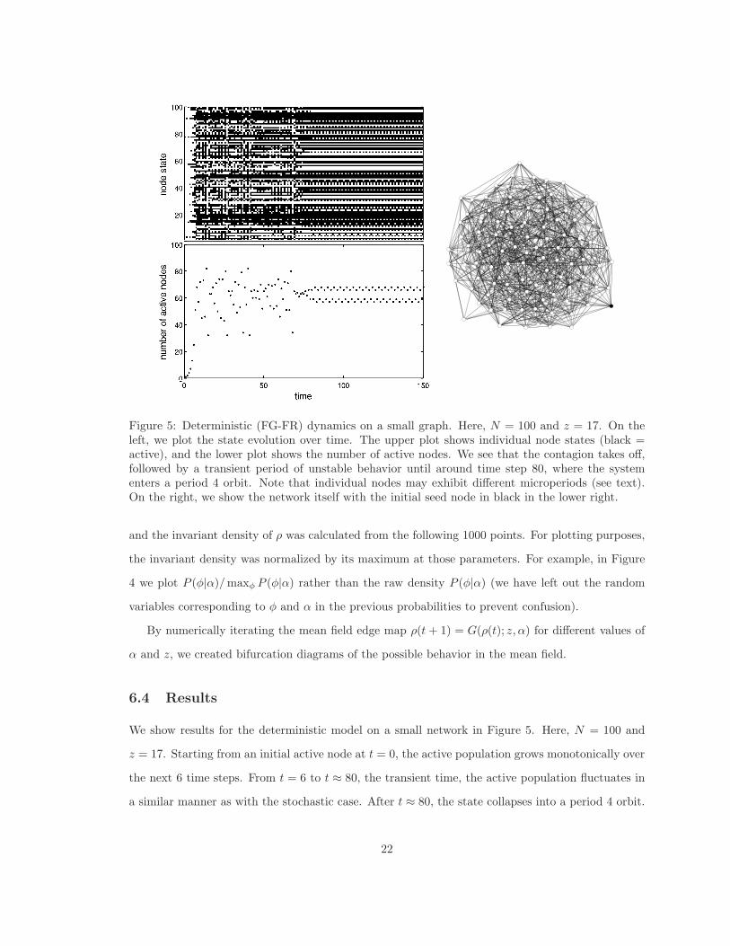
Figure 5: Deterministic (FG-FR) dynamics on a small graph. Here, N = 100 and z = 17. On theleft, we plot the state evolution over time. The upper plot shows individual node states (black =active), and the lower plot shows the number of active nodes. We see that the contagion takes off,followed by a transient period of unstable behavior until around time step 80, where the systementers a period 4 orbit. Note that individual nodes may exhibit different microperiods (see text).On the right, we show the network itself with the initial seed node in black in the lower right.
and the invariant density of ρ was calculated from the following 1000 points. For plotting purposes,
the invariant density was normalized by its maximum at those parameters. For example, in Figure
4 we plot P (φ|α)/maxφ P (φ|α) rather than the raw density P (φ|α) (we have left out the random
variables corresponding to φ and α in the previous probabilities to prevent confusion).
By numerically iterating the mean field edge map ρ(t+ 1) = G(ρ(t); z,α) for different values of
α and z, we created bifurcation diagrams of the possible behavior in the mean field.
6.4 Results
We show results for the deterministic model on a small network in Figure 5. Here, N = 100 and
z = 17. Starting from an initial active node at t = 0, the active population grows monotonically over
the next 6 time steps. From t = 6 to t ≈ 80, the transient time, the active population fluctuates in
a similar manner as with the stochastic case. After t ≈ 80, the state collapses into a period 4 orbit.
22
We call the overall period of the system its “macroperiod”. Individual nodes may exhibit different
“microperiods”. Note that the macroperiod is the lowest common multiple of the individual nodes’
microperiods. In Figure 5, we observe microperiods 1, 2, and 4. The focus of this thesis has been the
analysis of the on-off threshold model, and the deterministic (FG-FR) case has not been as amenable
to analysis as the stochastic cases. A deeper examination through simulation of the deterministic
case will appear in Dodds et al. (2012).
We explore the mean field dynamics by examining the limiting behavior of the active edge fraction
ρ under the map G(ρ; z,α). The map dynamics were simulated for a mesh of points in the (z,α)
plane. We plotted the 3-dimensional (3-d; N -d is N -dimensional for any integer N) bifurcation
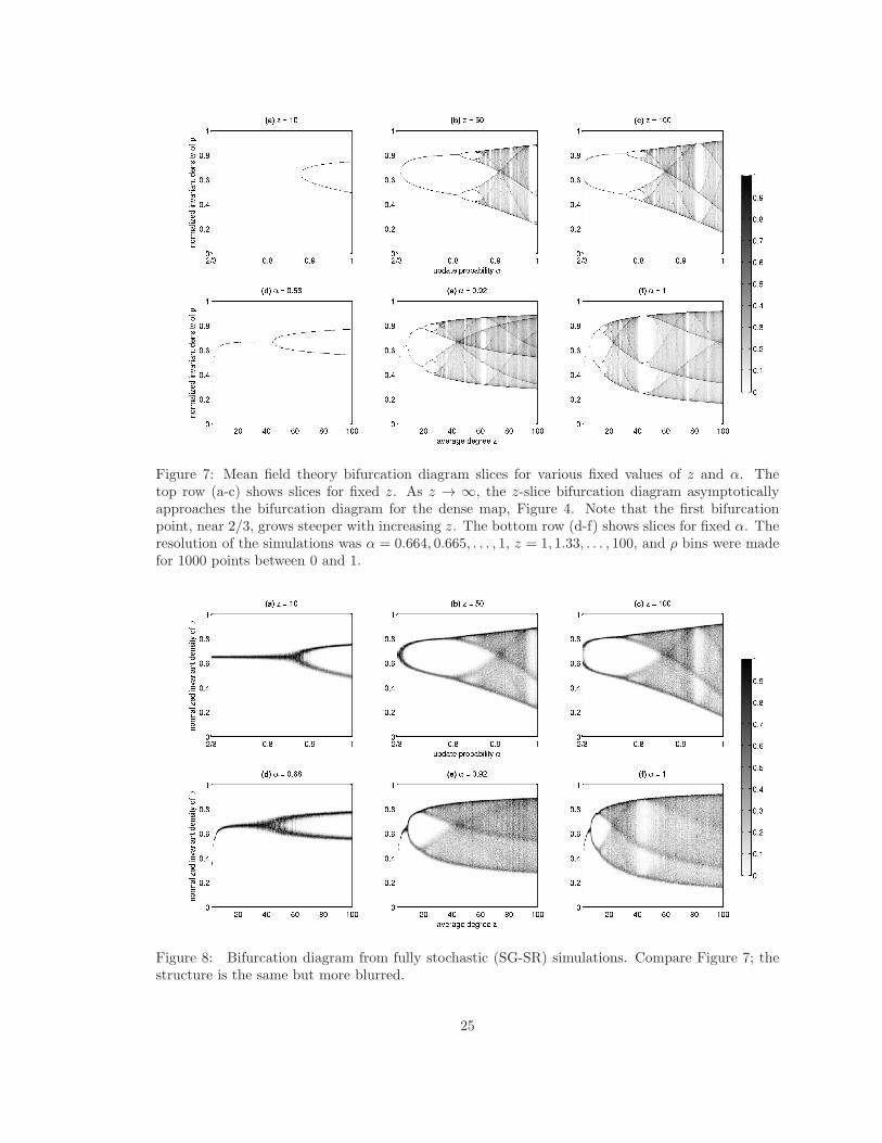
structure of the mean field theory in Figure 6. We also made 2-d bifurcation plots for fixed z and α
slices through this volume, Figures 7 and 8. In all cases, the invariant density of ρ is normalized by
its maximum for that (z,α) pair and indicated by the greyscale value.
The mean field map dynamics exhibit period-doubling bifurcations in both parameters z and α.
Visualizing the bifurcation structure in 3-d (Figure 6) shows interlacing period-doubling cascades in
the two parameter dimensions. These bifurcations are more clearly resolved when we take slices of
the volume for fixed parameter values. The mean field theory (Figure 7) closely matches the SG-SR
simulations (Figure 8). Since the first derivative G′ < Φ′ for any finite z, the bifurcation point
α = 2/3 which we found for the dense map Φ is an upper bound for the first bifurcation point of G.
The actual location of the first bifurcation point depends on z, but α = 2/3 becomes more accurate
for higher z (in Figures 6c and 7c, z = 100, and it is an excellent approximation). When α = 1, the
first bifurcation point occurs at z ≈ 7.
The bifurcation diagram slices resemble each other and evidently fall into the same universality
class as the logistic map (Feigenbaum, 1978, 1979). This class contains all 1-d maps with a sin-
gle, locally-quadratic maximum. Due to the properties of the Bernstein polynomials, Fk(ρ; f) will
universally have such a quadratic maximum for any concave, continuous f (Phillips, 2003). So this
will also be true for g(ρ; z, f) with z finite, and we see that z partially determines the amplitude
of that maximum, as in Figure 3. Thus z acts as a bifurcation parameter. The parameter α tunes
between G(ρ; z, 1) = g(ρ; z, f) and G(ρ; z, 0) = ρ, so it has a similar effect. Note that the tent
map f and the dense limit map Φ are kinked at their maxima, so their bifurcation diagrams are
qualitatively different from those of the mean field. The network, by constraining the interactions
among the population, causes the mean field behavior to fall into a different universality class than
23
Figure 6: The 3-dimensional bifurcation diagram computed from the mean field theory. The axes X= z, Y = α, Z = ρ are provided to orient the reader. The discontinuities of the surface are due tothe limited resolution of our simulations. See Figure 7 for the parameters used. This was plotted inParaview.
24
Figure 7: Mean field theory bifurcation diagram slices for various fixed values of z and α. Thetop row (a-c) shows slices for fixed z. As z → ∞, the z-slice bifurcation diagram asymptoticallyapproaches the bifurcation diagram for the dense map, Figure 4. Note that the first bifurcationpoint, near 2/3, grows steeper with increasing z. The bottom row (d-f) shows slices for fixed α. Theresolution of the simulations was α = 0.664, 0.665, . . . , 1, z = 1, 1.33, . . . , 100, and ρ bins were madefor 1000 points between 0 and 1.
Figure 8: Bifurcation diagram from fully stochastic (SG-SR) simulations. Compare Figure 7; thestructure is the same but more blurred.
25
the response function map.
7 Conclusions
We constructed the on-off threshold model as a simple model for social behavior as influenced by
others. This model allows us to study the effects of differing amounts of fixedness in the social
network and individual response functions. A detailed mean-field theory was then developed and
applied to a specific case, where the network is Poisson and the response functions average to the
tent map.
The model is rich in interesting mathematical behavior. The deterministic case, which we have
barely touched on here, merits further study. In particular, we would like to characterize the
distribution of periodic sinks, how the collapse time scales with system size, and how similar the
transient dynamics are to the mean-field dynamics.
Furthermore, the model should be tested on realistic networks. These could include power law
or small world random graphs, or real social networks gleaned from data.
Finally, the ultimate validation of this model would emerge from a better understanding of social
dynamics themselves. Characterization of people’s true response functions is therefore critical. This
might lead to more complicated context- and history-dependent models. Comparison of model
output to large data sets, such as data generated by social media, may provide an area for further
experimentation.
26
References
Aldana, M., Coppersmith, S., and Kadanoff, L. P. (2003). Boolean dynamics with ran-dom couplings. In Kaplan, E., Marsden, J. E., and Sreenivasan, K. R., editors, Per-spectives and Problems in Nonlinear Science, chapter 2, pages 23–90. Springer, New York.http://arxiv.org/abs/nlin/0204062.
Alligood, K. T., Sauer, T. D., and Yorke, J. A. (1996). Chaos: An Introduction to DynamicalSystems. Springer.
Bollobas, B. (2001). Random Graphs. Cambridge University Press, 2nd edition.
Chung, F. and Lu, L. (2002). The average distances in random graphs with give expected degrees.PNAS, 99(25):15879–15882.
Derrida, B. and Pomeau, Y. (1986). Random networks of automata: A simple annealed approxima-tion. Europhys. Lett., 1(2):45–49.
Dodds, P. S., Harris, K. D., and Danforth, C. M. (2012). Limited Imitation Contagion on RandomNetworks: Chaos, Universality, and Unpredictability. In preparation.
Dodds, P. S., Harris, K. D., and Payne, J. L. (2011). Direct, physically motivated derivation ofthe contagion condition for spreading processes on generalized random networks. Phys. Rev. E,83:056122.
Dodds, P. S. and Watts, D. J. (2004). Universal behavior in a generalized model of contagion. Phys.Rev. Lett., 92(21):218701.
Feigenbaum, M. J. (1978). Quantitative universality for a class of nonlinear transformations. Journalof Statistical Physics, 19(1):25–52.
Feigenbaum, M. J. (1979). The universal metric properties of nonlinear transformations. Journal ofStatistical Physics, 21(6):669–706.
Gleeson, J. P. (2008). Cascades on correlated and modular random networks. Phys. Rev. E,77:046117.
Gleeson, J. P. and Cahalane, D. J. (2007). Seed size strongly affects cascades on random networks.Phys. Rev. E, 75:056103.
Granovetter, M. (1978). Threshold models of collective behavior. American Journal of Sociology,83(6):1420–1443.
Granovetter, M. and Soong, R. (1986). Threshold models of interpersonal effects in consumerdemand. Journal of Economic Behavior and Organization, 7:83–99.
Hackett, A. W. (2011). Cascade Dynamics on Complex Networks. PhD thesis, University of Limerick.
Harris, T. E. (1963). The Theory of Branching Processes. Number 119 in Die Grundlehren derMathematischen Wissenschaften. Springer-Verlag, Berlin.
Kauffman, S. A. (1969). Metabolic stability and epigenesis in randomly constructed genetic nets.Journal of Theoretical Biology, 22:437–467.
Knuth, D. E. (1976). Big omicron and big omega and big theta. SIGACT News, 8(2):18–24.
Melnik, S., Hackett, A., Porter, M. A., Mucha, P. J., and Gleeson, J. P. (2011). The unreasonableeffectiveness of tree-based theory for networks with clustering. Phys. Rev. E, 83(3):036112.
Molloy, M. and Reed, B. (1995). A critical point for random graphs with a given degree sequence.Random Structures and Algorithms, 6:161–179.
Molloy, M. and Reed, B. (1998). The size of the giant component of a random graph with a givendegree sequence. Combinatorics Probability and Computing, 7(3):295–305.
Newman, M. E. J. (2003). The structure and function of complex networks. SIAM Review, 45(2):167–256.
NIST (2012). Digital Library of Mathematical Functions. http://dlmf.nist.gov.
Oliveira, R. I. (2010). Concentration of the adjacency matrix and of the Laplacian in random graphswith independent edges. http://arxiv.org/abs/0911.0600.
Payne, J. L., Harris, K. D., and Dodds, P. S. (2011). Exact solutions for social and biologicalcontagion models on mixed directed and undirected, degree-correlated random networks. Phys.Rev. E, 84:016110.
Pena, J. M., editor (1999). Shape Preserving Representations in Computer-Aided Geometric Design.Nova Science Publishers, Inc.
Phillips, G. M. (2003). Interpolation and Approximation by Polynomials. Springer. See chapter 7.
Schelling, T. C. (1971). Dynamic models of segregation. Journal of Mathematical Sociology, 1:143–186.
Schelling, T. C. (1973). Hockey helmets, concealed weapons, and daylight saving. Journal of ConflictResolution, 17(3):381–428.
Simmel, G. (1957). Fashion. American Journal of Sociology, 62(6):541–559.
Vespignani, A. (2012). Modelling dynamical processes in complex socio-technical systems. NaturePhysics, 8:32–39.
Watts, D. J. (2002). A simple model of global cascades on random networks. PNAS, 99(9):5766–5771.
West, D. B. (2001). Introduction to Graph Theory. Prentice Hall, Upper Saddle River, NJ, 2ndedition.
Winkler, R. L., Roodman, G. M., and Britney, R. R. (1972). The determination of partial moments.Management Science, 19(3):290–296.
Lemma 1. For k ≥ 1, let fk be continuous real-valued functions on a compact domain X withfk → f uniformly. Let qk be a probability mass function on Z+ parametrized by its mean z and withstandard deviation σ(z), assumed to be o(z). Then,
limz→∞
(
∞∑
k=0
qkfk
)
= f.
Proof. Suppose 0 ≤ α < 1 and let K = /z − zα0. Then,
g =∞∑
k=0
qkfk =K∑
k=0
qkfk +∞∑
k=K+1
qkfk. (A.1)
Since fk → f uniformly as k → ∞, for any ε > 0 we can choose z large enough that
|fk(x)− f(x)| < ε (A.2)
for all k > K and all x ∈ X. Without loss of generality, assume that |fk| ≤ 1 for all k. Then,
|g − f | ≤( σ
zα
)2+ ε.
The σ/zα term is a consequence of the Chebyshev inequality applied to the first sum in (A.1). Sinceσ grows sublinearly in z, this term vanishes for some 0 ≤ α < 1 when we take the limit z → ∞. Theε term comes from the second sum in (A.1) and (A.2), and it can be made arbitrarily small.
Appendix B Online material
To better explore the 3-d mean field bifurcation structure, we created movies of the the z and αslices as the parameters are dialed. The videos are available athttp://www.uvm.edu/~kharris/on-off-threshold/bifurc_movies.zip.Also, a VTK file with the 3-d bifurcation data, viewable in Paraview is athttp://www.uvm.edu/~kharris/on-off-threshold/volume_normalized.vtk.zip.
Videos of the individual-node dynamics for small networks in the FG-FR and FG-SR cases areshown for some parameters which produce interesting behavior. These are available athttp://www.uvm.edu/~kharris/on-off-threshold/graph_movies.zip.
The FG-FR, FG-SR, and SG-SR cases were implemented in Python. The code is available athttp://www.uvm.edu/~kharris/on-off-threshold/code.zip.