ON OPTIMAL INFERENCE IN THE LINEAR IV MODEL By Donald W. K. Andrews, Vadim Marmer, and Zhengfei Yu January 2017 Revised February 2018 COWLES FOUNDATION DISCUSSION PAPER NO. 2073R COWLES FOUNDATION FOR RESEARCH IN ECONOMICS YALE UNIVERSITY Box 208281 New Haven, Connecticut 06520-8281 http://cowles.yale.edu/
Transcript
ON OPTIMAL INFERENCE IN THE LINEAR IV MODEL
By
Donald W. K. Andrews, Vadim Marmer, and Zhengfei Yu
�Andrews gratefully acknowledges the research support of the National Science Foundation via grant numbers SES-1355504 and SES-1656313. Marmer gratefully acknowledges the research support of the SSHRC via grant numbers410-2010-1394 and 435-2013-0331. The authors thank Marcelo Moreira, James MacKinnon, a co-editor, and threereferees for helpful comments.
Abstract
This paper considers tests and con�dence sets (CS�s) concerning the coe¢ cient on the endogenous vari-
able in the linear IV regression model with homoskedastic normal errors and one right-hand side endogenous
variable. The paper derives a �nite-sample lower bound function for the probability that a CS constructed
using a two-sided invariant similar test has in�nite length and shows numerically that the conditional like-
lihood ratio (CLR) CS of Moreira (2003) is not always �very close,� say :005 or less, to this lower bound
function. This implies that the CLR test is not always very close to the two-sided asymptotically-e¢ cient
(AE) power envelope for invariant similar tests of Andrews, Moreira, and Stock (2006) (AMS).
On the other hand, the paper establishes the �nite-sample optimality of the CLR test when the correlation
between the structural and reduced-form errors, or between the two reduced-form errors, goes to 1 or -1 and
other parameters are held constant, where optimality means achievement of the two-sided AE power envelope
of AMS. These results cover the full range of (non-zero) IV strength.
The paper investigates in detail scenarios in which the CLR test is not on the two-sided AE power
envelope of AMS. Also, theory and numerical results indicate that the CLR test is close to having greatest
average power, where the average is over a grid of concentration parameter values and over pairs alternative
hypothesis values of the parameter of interest, uniformly over pairs of alternative hypothesis values and
uniformly over the correlation between the structural and reduced-form errors. Here, �close�means :015 or
less for k � 20; where k denotes the number of IV�s, and :025 or less for 0 < k � 40:The paper concludes that, although the CLR test is not always very close to the two-sided AE power
envelope of AMS, CLR tests and CS�s have very good overall properties.
Keywords: Conditional likelihood ratio test, con�dence interval, in�nite length, linear instrumental
variables, optimal test, weighted average power, similar test.
JEL Classi�cation Numbers: C12, C36.
1 Introduction
The linear instrumental variables (IV) regression model is one of the most widely used models
in economics. It has been widely studied and considerable e¤ort has been made to develop good
estimation and inference methods for it. In particular, following the recognition that standard two
stage least squares t tests and con�dence sets (CS�s) can perform quite poorly under weak IV�s
(see Dufour (1997), Staiger and Stock (1997), and references therein), inference procedures that
are robust to weak IV�s have been developed, e.g., see Kleibergen (2002) and Moreira (2003, 2009).
The focus has been on models with one right-hand side (rhs) endogenous variable, because this
arises most frequently in applications, and on over-identi�ed models, because Anderson and Rubin
(1949) (AR) tests and CS�s are robust to weak IV�s and perform very well in exactly-identi�ed
models.
Andrews, Moreira, and Stock (2006) (AMS) develop a �nite-sample two-sided AE power en-
velope for invariant similar tests concerning the coe¢ cient on the rhs endogenous variable in the
linear IV model under homoskedastic normal errors and known reduced-form variance matrix. They
show via numerical simulations that the conditional likelihood ratio (CLR) test of Moreira (2003)
has power that is essentially (i.e., up to simulation error) on the power envelope. Chernozhukov,
Hansen, and Jansson (2009) (CHJ) show that this power envelope also applies to non-invariant
tests provided the envelope is for power averaged over certain direction vectors in a unit sphere.
CHJ also shows that the invariant similar tests that generate the two-sided AE power envelope
are �-admissible and d-admissible. Mikusheva (2010) provides approximate optimality results for
CLR-based CS�s that utilize the testing results in AMS. Chamberlain (2007), Andrews, Moreira,
and Stock (2008), and Hillier (2009) provide related results.
It is shown in Dufour (1997) that any CS with correct size 1�� must have positive probabilityof having in�nite length at every point in the parameter space. The AR and CLR CS�s have this
property. In fact, simulation results show that in some over-identi�ed contexts the AR CS has
a lower probability of having an in�nite length than the CLR CS does. For example, consider a
model with one rhs endogenous variable, k IV�s, a concentration parameter �v (which is a measure
of the strength of the IV�s), homoskedastic normal errors, a correlation �uv between the structural-
equation error and the reduced-form error (for the �rst-stage equation) equal to zero, and no
covariates. When (k; �v) equals (2; 7); (5; 10); (10; 15); (20; 15); and (40; 20); the di¤erences between
the probabilities that the 95% CLR and AR CS�s have in�nite length are :013; :027; :037; :043;
and :049; respectively.1 In fact, one obtains positive di¤erences for all combinations of (k; �v) for
k = 2; 5; 10; 20; 40 and �v = 1; 5; 10; 15; 20: Hence, in these over-identi�ed scenarios the AR CS1See Table SM-I in the Supplemental Material for other parameter combinations.
1
outperforms the CLR CS in terms of its in�nite-length behavior, which is an important property
for CS�s. Similarly, one obtains positive (but smaller) di¤erences also when �uv = :3 for the same
range of (k; �v) values. On the other hand, for �uv = :5; :7; and :9; the di¤erences are negative over
the same range of (k; �v) values.
The AR and CLR CS�s are based on inverting AR and CLR tests that fall into the class of
invariant similar tests considered in AMS. Hence, the simulation results for �uv = :0 and :3 raise
the question: how can these results be reconciled with the near optimal CLR test and CS results
described above? In this paper, we answer this question and related questions concerning the
optimality of the CLR test and CS.
The contributions of the paper are as follows. First, the paper shows that the probability that
an invariant similar CS has in�nite length for a �xed true parameter value �� equals one minus the
power against �� of the test used to construct the CS as the null value �0 goes to 1 or �1: Thisleads to explicit formulae for the probabilities that the AR and CLR CS�s have in�nite length.
Second, the paper determines a �nite-sample lower bound function on the probabilities that a
CS has in�nite length for CS�s based on invariant similar tests. This lower bound is obtained by
using the �rst result and �nding the limit of the power bound in AMS as the null value �0 goes
to 1 or �1: The lower bound function is found to be very simple. It is a function only of j�uvj;�v; and k: These results allow one to compare the probabilities that the AR and CLR CS�s have
in�nite length with the lower bound.
Third, simulation results show that the AR and CLR CS�s are not always close to the lower
bound. This is not surprising for the AR CS, but it is surprising for the CLR CS in light of the
AMS results. The probabilities that the CLR CS has in�nite length are found to be o¤ the lower
bound function by a magnitude that is decreasing in j�uvj; increasing in k; and are maximized over�v at values that correspond to somewhat weak IV�s, but not irrelevant IV�s. For �uv = 0; the paper
shows (analytically) that the AR test achieves the lower bound function. Hence, for �uv = 0; the
probabilities that the CLR CS has in�nite length exceed the lower bound by the same amounts as
reported above for the di¤erence between the in�nite length probabilities of the CLR and AR CS�s
for several (k; �v) values. On the other hand, for values of j�uvj � :7; the CLR CS has probabilities
of having in�nite length that are close to the lower bound function, :010 or less and typically much
less, for all (k; �v) combinations considered. For values of j�uvj � :7; the AR CS has probabilities
of having in�nite length that are often far from the lower bound. For j�uvj = :9 and certain values
of �v; they are as large as :084; :196; :280; :353; and :422 for k = 2; 5; 10; 20; and 40; respectively.2
The AMS numerical results did not detect scenarios where the CLR test�s power is o¤ the two-
2See Table SM-I in the SM.
2
sided power envelope because AMS focussed on power for a �xed null hypothesis and a wide range
of alternative values, whereas the probability that CS has in�nite length depends on underlying
tests�power for a �xed true parameter and arbitraily distant null hypothesis values. As discussed
in Section 4 below, power in these two scenarios is di¤erent.
AMS reports results for only two values of the correlation � between the reduced-form errors,
viz., � = :5 and :95: However, this is not the reason that AMS did not detect scenarios where the
CLR test�s power is noticeably o¤ the two-sided power envelope. Figure SM-I in the Supplemental
Material provides graphs that are the same as in AMS, but with � = 0; rather than � = :5 or :95:
Even for � = 0; the power of the CLR test is close to the POIS2 power envelope in the scenarios
considered, viz., :0110 or less. Note that � = 0 is the � value that yields many of the largest
di¤erences between the power of the CLR test and the POIS2 power envelope found in this paper
when the true �� = 0 is �xed and the null value �0 varies.
Fourth, the paper derives new optimality properties of the CLR and Lagrange multiplier (LM)
tests when �uv ! �1 or � ! �1 with other parameters �xed at any values (with non-zeroconcentration parameter). In particular, optimality holds for �xed �nite non-zero values of the
concentration parameter. Optimality here is in the class of invariant similar tests or similar tests
and employs the two-sided AE power envelope of AMS. These results are empirically relevant
because they are consistent with the numerical results that show that the CLR test is close to the
power envelope when j�uvj is large, viz., :7 and :9; but not extremely close to one.These optimality results hold because taking �uv ! �1 or � ! �1 with other parameters �xed
drives the length of the mean vector of the conditioning statistic T; as de�ned in AMS and below,
to in�nity. This is the same mechanism that yields asymptotic optimality of the CLR and LM tests
when the concentration parameter goes to in�nity as n ! 1 (i.e., under strong or semi-strong
IV�s). The results show that arbitrarily large values of the concentration parameter are not needed
for limiting optimality of the CLR and LM tests.
Fifth, we simulate power di¤erences (PD�s) between the two-sided AE power envelope of AMS
and the power of the CLR test for a �xed alternative value �� and a range of �nite null values
�0 (rather than the PD�s as �0 ! �1 discussed above). These PD�s are equivalent to the false
coverage probability di¤erences between the CLR CS and the corresponding infeasible optimal
CS for a �xed true value �� at incorrect values �0: We consider a wide range of (�0; �v; �uv; k)
values. The maximum (over �0 and �v values) PD�s range between [:016; :061] over the (�uv; k)
values considered. On the other hand, the average (over �0 and � values) PD�s only range between
[:002; :016]: This indicates that, although there are some (�0; �) values at which the CLR test is
noticeably o¤ the power envelope, on average the CLR test�s power is not far from the power
3
envelope. The maximum PD�s over (�0; �) are found to increase in k and decrease in j�uvj: The�v values at which the maxima are obtained are found to (weakly) increase with k and decrease
in j�uvj: The j�0j values at which the maxima are obtained are found to be independent of k anddecrease in j�uvj:
Sixth, the paper considers a weighted average power (WAP) envelope with a uniform weight
function over a grid of concentration parameter values �v and the same two-point AE weight
function over (�; �) as in AMS. We refer to this as the WAP2 envelope. We determine numerically
how close the power of the CLR test is to the WAP2 envelope. We �nd that the di¤erence between
the WAP2 envelope and the average power of the CLR test is in the range of [:001; :007] over all
of the (�0; ��; �uv; k) values that we consider. Hence, the average power of the CLR test is quite
close to the WAP2 envelope.
Other papers in the literature that consider WAP include Wald (1943), Andrews and Ploberger
(1994), Andrews (1998), Moreira and Moreira (2013), Elliott, Müller, and Watson (2015), and
papers referenced above. The WAP2 envelope considered here is closest to the WAP envelopes
in Wald (1943), AMS, and CHJ because the other papers listed put a weight function over all of
the parameters in the alternative hypothesis, which yields a single weighted alternative density. In
contrast, the WAP2 envelope, Wald (1943), AMS, and CHJ consider a family of weight functions
over disjoint sets of parameters in the alternative hypothesis, which yields a WAP envelope.
In conclusion, based on our �ndings, we recommend use of the CLR test and CS. More specif-
ically, we recommend using heteroskedasticity-robust versions of these procedures that have the
same asymptotic properties as these procedures under homoskedasticity. For example, such tests
are given in Andrews, Moreira, and Stock (2004) and Andrews and Guggenberger (2015). The
CLR CS has higher probability of having in�nite length than the AR CS in some scenarios, and
the CLR test is not a UMP two-sided invariant similar test. But, no such UMP test exists and the
CLR CS is close to the two-sided AE power envelope for invariant similar tests when j�uvj is notclose to zero and is close to the WAP2 envelope for all values of j�uvj:
Finally, we point out that the results of this paper illustrate a point that applies more generally
than in the linear IV model. In weak identi�cation scenarios, where CS�s may have in�nite length
(or may be bounded only due to bounds on the parameter space), good test performance at a priori
implausible parameter values is important for good CS performance at plausible parameter values.
More speci�cally, the probability under an a priori plausible parameter value �� that a CS has
in�nite length depends on the power of the test used to construct the CS against �� when the null
value j�0j is arbitrarily large, which may be an a priori implausible null value.For the computation of CLR CS�s, see Mikusheva (2010). For a formula for the power of the
4
CLR test, see Hillier (2009).
The paper is organized as follows. Section 2 speci�es the model. Section 3 de�nes the class of
invariant similar tests. Section 4 contrasts the power properties of tests in the scenario where �0
is �xed and �� takes on large (absolute) values, with the scenario where �� is �xed and �0 takes
on large (absolute) values. Section 5 provides a formula for the probability that a CS has in�nite
length. Section 6 derives a lower bound on the probability that a CS constructed using two-sided
invariant similar tests has in�nite length. Section 7 reports di¤erences between the probability
that the CLR CS has in�nite length and the lower bound derived in the previous section. Section
8 proves the optimality results for the CLR test described above. Section 9 reports di¤erences
between the power of CLR tests and the two-sided AE power bound of AMS for a wide range of
parameter con�gurations. Section 10 provides comparisons of the power of the CLR test to the
WAP2 power envelope described above. Proofs and additional theoretical and numerical results
are given in the Supplemental Material (SM).
2 Model
We consider the same model as in Andrews, Moreira, and Stock (2004, 2006) (AMS04,
AMS) but, for simplicity and without loss of generality (wlog), without any exogenous variables.
The model has one rhs endogenous variable, k instrumental variables (IV�s), and normal errors
with known reduced-form error variance matrix. The model consists of a structural equation and
a reduced-form equation:
y1 = y2� + u and y2 = Z� + v2; (2.1)
where y1; y2 2 Rn and Z 2 Rn�k are observed variables; u; v2 2 Rn are unobserved errors; and
� 2 R and � 2 Rk are unknown parameters. The IV matrix Z is �xed (i.e., non-stochastic) and
has full column rank k: The n� 2 matrix of errors [u:v2] is i.i.d. across rows with each row havinga mean zero bivariate normal distribution.
The two corresponding reduced-form equations are
Y := [y1 :y2] := [Z�� + v1 :Z� + v2] = Z�a0 + V; where
V := [v1 : v2] = [u+ v2� : v2]; and a := (�; 1)0: (2.2)
The distribution of Y 2 Rn�2 is multivariate normal with mean matrix Z�a0; independence acrossrows, and reduced-form variance matrix 2 R2�2 for each row. For the purposes of obtaining
exact �nite-sample results, we suppose is known. As in AMS, asymptotic results for unknown
5
and weak IV�s are the same as the exact results with known : The parameter space for � = (�; �0)0
is Rk+1:
We are interested in tests of the null hypothesis H0 : � = �0 and CS�s for �:
As shown in AMS, Z 0Y is a su¢ cient statistic for (�; �0)0: As in Moreira (2003) and AMS, we
consider a one-to-one transformation [S : T ] of Z 0Y :
S := (Z 0Z)�1=2Z 0Y b0 � (b00b0)�1=2 � N(c�(�0;) � ��; Ik) and
T := (Z 0Z)�1=2Z 0Y �1a0 � (a00�1a0)�1=2 � N(d�(�0;) � ��; Ik); where
d�(�0;) := b0b0 � (b00b0)�1=2 det()�1=2 2 R; and b = (1;��)0: (2.3)
As de�ned, S and T are independent. Note that S and T depend on the null hypothesis value �0:
3 Invariant Similar Tests
As in Hillier (1984) and AMS, we consider tests that are invariant to orthonormal transfor-
mations of [S : T ]; i.e., [S : T ] ! [FS : FT ] for a k � k orthogonal matrix F: The 2� 2 matrix Qis a maximal invariant, where
Q = [S:T ]0[S:T ] =
24 S0S S0T
S0T T 0T
35 =24 QS QST
QST QT
35 and Q1 =
0@ S0S
S0T
1A =
0@ QS
QST
1A ; (3.1)
e.g., see Theorem 1 of AMS. Note that Q1 is the �rst column of Q and the matrix Q depends on
the null value �0:
The statistic Q has a non-central Wishart distribution because [S :T ] is a multivariate normal
matrix that has independent rows and common covariance matrix across rows. The distribution of
Q depends on � only through the scalar
� := �0Z 0Z� � 0: (3.2)
Leading examples of invariant identi�cation-robust tests in the literature include the AR test,
the LM test of Kleibergen (2002) and Moreira (2009), and the CLR test of Moreira (2003). The
latter test depends on the standard LR test statistic coupled with a �conditional� critical value
6
that depends on QT . The LR, LM, and AR test statistics are
LR :=1
2
�QS �QT +
q(QS �QT )2 + 4Q2ST
�;
LM := Q2ST =QT = (S0T )2=T 0T; and AR := QS=k = S0S=k: (3.3)
The critical values for the LM and AR tests are �21;1�� and �2k;1��=k; respectively, where �
2m;1��
denotes the 1� � quantile of the �2 distribution with m degrees of freedom.
A test based on the maximal invariant Q is similar if its null rejection rate does not depend
on the parameter � that determines the strength of the IV�s Z: As in Moreira (2003), the class of
invariant similar tests is speci�ed as follows. Let the [0; 1]-valued statistic �(Q) denote a (possibly
randomized) test that depends on the maximal invariant Q: An invariant test �(Q) is similar with
signi�cance level � if and only if E�0(�(Q)jQT = qT ) = � for almost all qT > 0 (with respect to
Lebesgue measure), where E�0(�jQT = qT ) denotes conditional expectation given QT = qT when
� = �0 (which does not depend on �):
The CLR test rejects the null hypothesis when
LR > �LR;�(QT ); (3.4)
where �LR;�(QT ) is de�ned to satisfy P�0(LR > �LR;�(QT )jQT = qT ) = � and the conditional
distribution of Q1 = (QS ; QST )0 given QT is speci�ed in AMS and in (12.3) in the SM.
The invariance condition discussed above is a rotational invariance condition. In some cases,
we also consider a sign invariance condition. A test that depends on [S : T ] is sign invariant if it is
invariant to the transformation [S : T ] ! [�S : T ]: A rotation invariant test is also sign invariantif it depends on QST only through jQST j: Tests that are sign invariant are two-sided tests. In fact,AMS shows that the two-sided AE power envelope is identical to the power envelope generated by
sign and rotation invariant tests, see (4.11) in AMS.
For simplicity, we will use the term invariant test to mean a rotation invariant test and the term
sign and rotation invariant test to describe a test that satis�es both invariance conditions.
The paper also provides some results that apply to tests that satisfy no invariance properties.
A test �([S : T ]) (that is not necessarily invariant) is similar with signi�cance level � if and only if
E�0(�([S : T ])jT = t) = � for almost all t (with respect to Lebesgue measure), where E�0(�jT = t)
denotes conditional expectation given T = t when � = �0 (which does not depend on �); see
Moreira (2009).
7
4 Power Against Distant Alternatives Compared to Distant Null
Hypotheses
In this section, we consider the power properties of tests when j�� � �0j is large, where ��denotes the true value of �:We compare scenario 1; where �0 and are �xed and �� takes on large
(absolute) values, to scenario 2; where �� and are �xed and �0 takes on large (absolute) values.
Scenario 1 yields the power function of a test against distant alternatives. Scenario 2 yields the
false coverage probabilities of the CS constructed using the test for distant null hypotheses (from
the true parameter value ��). We show that, while power goes to one in scenario 1 as �� ! �1for �xed �0 for standard tests, it is not true that power goes to one in scenario 2 as �0 ! �1 for
�xed ��: Hence, the power properties of tests are quite di¤erent in scenarios 1 and 2.
The numerical power function and power envelope calculations in AMS are all of the type in
scenario 1: The di¤erence in power properties of tests between scenarios 1 and 2 suggests that it
is worth exploring the properties of tests in scenarios of the latter type as well. We do this in
the paper and show that the �nding of AMS that the CLR test is essentially on the two-sided AE
power envelope and is always at least as powerful as the AR test does not hold when one considers
a broader range of null and alternative hypothesis values (�0; ��) than considered in the numerical
results in AMS.
It is convenient to consider the AR test, which is the simplest test. The AR test rejects
H0 : � = �0 when S0S > �2k;�: When the true value is �; the distribution of the S
0S statistic is
noncentral �2 with noncentrality parameter
c2�(�0;) � � (4.1)
and k degrees of freedom. For the �xed null hypothesis H0 : � = �0; �xed ; and �xed �; the
power at the alternative hypothesis value �� is determined by c2��(�0;): We have
limj��j!1
c2��(�0;) = limj��j!1
(�� � �0)2 � (b00b0)�1 =1: (4.2)
Hence, the power of the AR test goes to one as j��j ! 1:On the other hand, if one �xes the alternative hypothesis value �� and one considers the limit
8
as j�0j ! 1; then one obtains
limj�0j!1
c2��(�0;) = limj�0j!1
(�� � �0)2 � (b00b0)�1
= limj�0j!1
(�� � �0)2 � (!21 � 2!12�0 + !22�20)�1
= 1=!22; (4.3)
where !21; !22; and !12 denote the (1; 1); (2; 2); and (1; 2) elements of ; respectively. Hence, the
power of the AR test does not go to one as j�0j ! 1 even though j�0 � ��j ! 1: This occursbecause the structural equation error variance, V ar(ui) = b00b0; diverges to in�nity as j�0j ! 1:
The di¤ering results in (4.2) and (4.3) is easy to show for the AR test, but it also holds for
Kleibergen�s and Moreira�s LM test and Moreira�s CLR test. For brevity, we do not provide such
results here.
Note that Davidson and MacKinnon (2008, Sec. 4) provide di¤erent, but somewhat related,
results to those in this section.3 They consider power when �0 is �xed and �� takes on large
(absolute) values (as in scenario 1) but when the correlation �uv (between the structural-equation
error u and the reduced-form error v2) is held �xed and the structural equation error variance is
estimated. In contrast, the results given here are for the case where the correlation � (between the
reduced-form errors v1 and v2) is held �xed because � can be consistently estimated and, hence,
in large samples can be treated as �xed and known. This is not true for �uv: In the Davidson and
MacKinnon (2008) scenario, power does not go to one as �� ! �1 for �xed �0:
5 Probability That a Con�dence Set Has In�nite Length
In this section, we show that the probability that a CS has in�nite length is given by one minus
the power of the test used to construct the CS as the null value �0 of the test goes to 1 or �1:This provides motivation for interest in the power of tests as �0 ! �1: It shows why high poweragainst distant null hypotheses is highly desirable.
We sometimes make the dependence of Q; S; and T on Y and �0 explicit and write
We denote the (1; 1); (1; 2); and (2; 2) elements of Q�0(Y ) by QS;�0(Y ); QST;�0(Y ); and QT;�0(Y );
respectively.
3Davidson and MacKinnon (2008) do not consider the probabilities of unbounded CS�s or provide optimalityresults for tests, which are the main focus of this paper.
9
Let
�(Q�0(Y )) = 1(T (Q�0(Y )) > cv(QT�0(Y ))) (5.2)
be a (nonrandomized) invariant similar level � test for testing H0 : � = �0 for �xed known ;
where T (Q�0(Y )) is a test statistic and cv(QT�0(Y )) is a (possibly data-dependent) critical value.Examples include the AR, LM, and CLR tests in (3.3). Let CS� be the level 1�� CS correspondingto �: That is,
CS�(Y ) = f�0 : �(Q�0(Y )) = 0g: (5.3)
We say CS�(Y ) has right (or left) in�nite length, which we denote by RLength(CS�(Y )) =1(or LLength(CS�(Y )) =1), if
9K(Y ) <1 such that � 2 CS�(Y ) 8� � K(Y ) (or 8� � �K(Y )): (5.4)
We say CS�(Y ) has in�nite length, which we denote by Length(CS�(Y )) =1; if it has right andleft in�nite lengths. A CS with in�nite length contains a set of the form (�1;K1(Y ))[(K2(Y );1)for some �1 < K1(Y ) � K2(Y ) <1:
Let P��;�;(�) denote probability for events determined by Y when Y has a multivariate normaldistribution with means matrix [��� : �] 2 R2k; independence across rows, and variance matrix for each row. Let P��;�0;�;(�) denote probability for events determined by Q when Q := [S : T ]
0[S :
T ] and [S : T ] has the multivariate normal distribution in (2.3) with � = �� and � = �0���: In this
case, Q has a noncentral Wishart distribution whose density is given in (12.2) in the SM.
For �xed true value �� and reduced-form variance matrix ; let �� denote the corresponding
structural variance matrix of each row of [u : v2]: Let �uv denote the correlation between the
structural and reduced-form errors, i.e., the correlation corresponding to ��: Some calculations
show that
�uv =!12 � !22��
(!21 � 2!12�� + !22�2�)1=2!2and
�� =
24 �2u �u�v�uv
�u�v�uv �2v
35 =24 !21 � 2!12�� + !22�2� !12 � !22��
!12 � !22�� !22
35 ; (5.5)
where !21; !22; and !12 the elements of ; see (12.9) in the SM. By the �rst equality in the second
line of (5.5), �2u = V ar(ui); �2v = V ar(v2i); and �uv = Corr(ui; v2i):
10
It is shown in Lemma 16.1 in the SM that the limit as �0 ! �1 of Q�0(Y ) is
Q�1(Y ) :=
24 e02Y0PZY e2 � 1�2v e02Y
0PZY �1e1 � �(1��
2uv)
1=2�u�v
e02Y0PZY
�1e1 � �(1��2uv)
1=2�u�v
e01�1Y 0PZY
�1e1 � (1� �2uv)�2u
35 ; (5.6)
where PZ := Z(Z 0Z)�1Z 0; e1 := (1; 0)0; and e2 := (0; 1)0: Let QT;�1(Y ) denote the (2; 2) element
of Q�1(Y ): It is also shown in Lemma 16.1 in the SM that Q�1(Y ) has a noncentral Wishart
distribution with means matrix ���(1=�v; �uv=(�v(1 � �2uv)1=2)) 2 Rk�2 and identity variance
matrix.4
Theorem 5.1 Suppose CS�(Y ) is a CS based on invariant level � tests �(Q�0(Y )) whose test
statistic and critical value functions, T (q) and cv(qT ); respectively, are continuous at all positivede�nite 2 � 2 matrices q and positive constants qT ; P��;�;(T (Qc(Y )) = cv(QT;c(Y ))) = 0 for
c = +1 in parts (a) and (c) below and c = �1 in part (b) below. Then, for all (��; �;);
(c) if the tests are sign invariant, i.e., T (Q) depends on QST only through jQST j; thenP��;�;(Length(CS�(Y )) =1) = 1� lim�0!�1 P��;�0;�;(�(Q) = 1):
Comments. (i). For the AR, LM, and LR tests, the continuity conditions on T (q) and cv(qT )hold given their simple functional forms in (3.3) using the assumption that qT > 0 for the LM
statistic and using the continuity of �LR;�(qT ); which holds by the argument in the proof of Thm.
10.1 in Andrews and Guggenberger (2016). We have P��;�;(T (Q�1(Y )) = cv(QT;�1(Y ))) = 0 for
the AR and LM tests because cv(QT;�1(Y )) is a constant and T (Q�1(Y )) is absolutely continuouswith respect to Lebesgue measure. For the CLR test, P��;�;(T (Q�1(Y )) = cv(QT;�1(Y ))) = 0 by
the argument given in the proof of Theorem 6.4 in the SM. The AR, LM, and CLR test statistics are
sign invariant. Hence, parts (a)-(c) of Theorem 5.1 apply to these tests. Theorem 6.4(a)-(c) below
provides formulae for the quantities lim�0!�1 P��;�0;�;(�(Q) = 1); which appear in Theorem 5.1,
for the AR, LM, and CLR tests.
(ii). Comment (iii) to Theorem 6.2 below provides a lower bound on 1�lim�0!1 P��;�0;�;(�(Q)
= 1) over all sign and rotation invariant similar level � tests. Combining this with Theorem 5.1(c)
yields a lower bound on the probability that a CS CS�(Y ) based on such tests has Length = 1:The lower bound on the probability that Length = 1 is greater than the lower bound on the
probability that RLength =1 (or that LLength =1) unless �uv = 0 (in which case it turns outthat they are equal).
4The density of this distribution is given in (12.4) in the SM.
11
Theorem 13.1 in the SM provides lower bounds on 1� lim�0!�1 P��;�0;�;(�(Q) = 1) over all
invariant similar level � tests. Combining these with Theorem 5.1(a) and (b) yields lower bounds
on the probabilities that a CS CS�(Y ) has RLength = 1 based on �0 ! 1 and LLength = 1based on �0 ! �1:
(iii). Note that Theorem 5.1 does not impose similarity, just invariance. The results of Theorem
5.1(a) and (b) also hold for a CS�(Y ) that is based on level � tests that are not invariant. Denote
such tests by �(S�0(Y ); T�0(Y )) and suppose their test statistic and critical value functions, T (s; t)and cv(t); respectively, are continuous at all k � 2 matrices [s : t] and k vectors t and satisfy
1) = 1� lim�0!1 P��;�0;�;(�([S : T ]) = 1) and likewise with LLength(�); �0 ! �1; and c = �1in place of RLength(�); �0 !1; and c = +1: If, in addition, the tests satisfy: T (Sc(Y ); Tc(Y )) �cv(Tc(Y )) for c = +1 i¤ the same inequality holds for c = �1; then Theorem 5.1(c) also holds.
(These results hold by a straightforward modi�cation of the proof of Theorem 5.1.)
(iv). By Dufour (1997), all CS�s for � with correct size must have positive probability of
having in�nite length (assuming � is not bounded away from 0). In consequence, expected CS
length, which is a standard measure of the performance of a CS, is in�nite for all identi�cation-
robust CS�s. Due to this, Mikusheva (2010) compares CS�s based on their expected truncated
lengths for various truncation values. The result of Theorem 6.2 below implies that, for two CS�s
where the rhs of Theorem 6.2(c) is smaller for the �rst CS than the second, the �rst CS has smaller
expected truncated length than the second for su¢ ciently large truncation values.
(v) Section 25 in the Supplemental Material extends Theorem 5.1 to the linear IV model that
allows for heteroskedasticity and autocorrelation (HC) in the errors, as in Moriera and Ridder
(2017).
6 Power Bound as �0! �1
In this section, we provide two-sided AE power bounds for invariant similar tests as �0 ! �1for �xed ��:We obtain these bounds by �nding the limit of the power bounds in Theorem 3 of AMS
as �0 ! �1: The power bounds also apply to the larger class of similar tests for which invarianceis not imposed, provided power is averaged over ��=jj��jj vectors using the uniform distribution onthe unit sphere in Rk; as in CHJ.
Using Theorem 5.1, these results are used to obtain bounds on the probabilities that CS�s
constructed using sign and rotation invariant similar tests have in�nite length. They also are used
12
to obtain bounds on certain average probabilities that similar invariant tests and similar tests have
in�nite right (or left) length.
This section also determines the power of the AR, LM, and CLR tests as �0 ! �1 and the
probabilities that AR, LM, and CLR CS�s have in�nite length.
6.1 Density of Q as �0! �1
The density of Q := [S : T ]0[S : T ] when [S : T ] has the multivariate normal distribution in (2.3)
only depends on � through � := �0���: Let fQ(q;��; �0; �;) denote this density when � = ��:
It is a noncentral Wishart density with means matrix of rank one and identity covariance matrix,
which was �rst derived by Anderson (1946, eqn. (6)). An explicit expression for fQ(q;��; �0; �;)
is given in (12.2) in the SM.
Now, we determine the limit of the density fQ(q;��; �0; �;) as �0 ! �1: De�ne
ruv :=�uv
(1� �2uv)1=2and �v := �=�2v = �0���=�
2v: (6.1)
Note that �v is the concentration parameter, which indexes the strength of the IV�s. Let
fQ(q; �uv; �v) denote the density of Q := [S : T ]0[S : T ] when [S : T ] has a multivariate nor-
mal distribution with means matrix
�� � (1=�v; ruv=�v) 2 Rk�2; (6.2)
all variances equal to one, and all covariances equal to zero. This density also is a noncentral Wishart
density with means matrix of rank one and identity covariance matrix. The density depends on
ruv; �v; and � only through �uv and �v: An explicit expression for fQ(q; �uv; �v) is given in (12.4)
in Section 12.1 the SM.
Lemma 6.1 For any �xed (��; �;); lim�0!�1 fQ(q;��; �0; �;) = fQ(q; �uv; �v) for all 2 � 2variance matrices q; where �uv and �v are de�ned in (5.5) and (6.1), respectively.
Comment. Lemma 6.1 is proved by showing: lim�0!�1 c��(�0;) = �1=�v and lim�0!�1d��(�0;) = � !22���!12
!2(!21!22�!212)1=2
= � �uv�v(1��2uv)1=2
; see Lemma 15.1 in the SM. When expressed in
terms of ��; the latter limit only depends on �uv; �u; and �v and its functional form is of a
relatively simple multiplicative form.
Let P��;�0;�;(�) and P�uv ;�v(�) denote probabilities under the alternative hypothesis densitiesfQ(q;��; �0; �;) and fQ(q; �uv; �v); respectively, de�ned above.
13
6.2 Two-Sided AE Power Bound as �0! �1
AMS provides a two-sided power envelope for invariant similar tests based on maximizing av-
erage power against two points in the alternative hypothesis: (��; �) and (�2�; �2): AMS refers to
this as the two-sided AE power envelope because given one point (��; �); the second point (�2�; �2)
is the unique point such that the test that maximizes average power against these two points is a
two-sided AE test under strong IV asymptotics. This power envelope is a function of (��; �):
Given (��; �); the second point (�2�; �2) satis�es
�2� = �0 �d�0(�� � �0)
d�0 + 2r�0(�� � �0)and �2 = �
(d�0 + 2r�0(�� � �0))2
d2�0; (6.3)
where r�0 := e01�1a0 � (a00�1a0)�1=2; see (4.2) of AMS. We let POIS2(Q;�0; ��; �) denote the
optimal average-power test statistic for testing � = �0 against (��; �) and (�2�; �2): Its condi-
tional critical value is denoted by �2;�0(QT ): For brevity, the formulas for POIS2(Q;�0; ��; �) and
�2;�0(QT ) are given in Section 17 in the SM.
The limit as �0 ! �1 of the POIS2(Q;�0; ��; �) statistic is shown in (17.6) in the SM to be
2(QT ; j�uvj; �v) := exp(��vr2uv=2)(�vr2uvQT )�(k�2)=4I(k�2)=2(p�vr2uvQT ); and
�(Q; �uv) := QS + 2ruvQST + r2uvQT ; (6.4)
where Q; QS ; QST ; and QT are de�ned in (3.1), �uv is de�ned in (5.5), ruv and �v are de�ned in
(6.1), and I�(�) denotes the modi�ed Bessel function of the �rst kind of order � (e.g., see Comment(ii) to Lemma 3 of AMS for more details regarding I�(�)):
Let �2;1(qT ) denote the conditional critical value of the POIS2(Q;1; j�uvj; �v) test statistic.That is, �2;1(qT ) is de�ned to satisfy
for all qT � 0; where PQ1jQT (�jqT ) denotes probability under the null density fQ1jQT (�jqT ); which isspeci�ed explicitly in (12.3) in the SM and does not depend on �0:
When �uv = 0; the test based on POIS2(Q;1; j�uvj; �v) is the AR test. This follows because�(Q; 0) = QS ; (Q; 0; �v) is monotone increasing in �(Q; 0); and 2(QT ; 0; �v) is a constant. Some
intuition for this is that EQST = 0 under the null and limj�0j!1EQST = 0 under any �xed
14
alternative �� when �uv = 0:5 In consequence, QST is not useful for distinguishing between H0 and
H1 when j�0j ! 1 and �uv = 0: Furthermore, it is shown in (13.5) and Theorem 13.1 in the SM
that the AR test is also the best one-sided test as �0 ! +1 and as �0 ! �1:The following theorem shows that the POIS2(Q;1; j�uvj; �v) test provides a two-point average-
power bound as �0 ! �1 for any invariant similar test for any �xed (��; �) and :
Theorem 6.2 Let f��0(Q) : �0 ! �1g be any sequence of invariant similar level � tests of
H0 : � = �0 for �xed known : For �xed (��; �); (�2�; �2) de�ned (6.3), and ; the two-sided AE
power envelope test POIS2(Q;1; j�uvj; �v) de�ned in (6.4) and (6.5) satis�es
Comments. (i). The power bound in Theorem 6.2 only depends on (��; �); (�2�; �2); and
through j�uvj; which is the absolute magnitude of endogeneity under ��; and �v; which is the
concentration parameter.
(ii). The power bound in Theorem 6.2 is strictly less than one. Hence, it is informative.
(iii). For sign and rotation invariant similar tests ��0(Q); the lim sup on the left-hand side in
Theorem 6.2 is the average of two equal quantities.
(iv). Theorem 6.2 can be extended to cover sequences of similar tests f��0(S; T ) : �0 !�1g that satisfy no invariance properties, using the proof of Theorem 1 in CHJ. In this case,
the left-hand side (lhs) probabilities in Theorem 6.2 depend on � or, equivalently (�; ��=jj��jj);rather than just �: In this case, Theorem 6.2 holds with P��;�0;�;(��0(Q) = 1) replaced byRP��;�;��=jj�� jj;(��0(S; T ) = 1)dUnif(��=jj��jj) and analogously for the term that depends on
(�2�; �2); where P��;�;��=jj�� jj;(�) denotes probability under (��; �; ��=jj��jj;) and Unif(�) de-notes the uniform measure on the unit sphere in Rk:
6.3 Lower Bound on the Probability That a CS Has In�nite Length
Next, we combine Theorems 5.1 and 6.2 to provide a lower bound on the probability that a
sign and rotation invariant similar CS has in�nite length. The same lower bound applies to the
average probability over (��; �) and (�2�; �) that a rotation invariant similar CS has right (left)
5We have EQST = ES0ET by independence of S and T; EQST = 0 under H0 because ES = 0; andlimj�0j!1EQST = 0 under �� because ET = ��d��(�0;); lim�0!�1 d��(�0;)! �ruv=�v by Lemma 15.1(e) inthe SM, and ruv = 0 when �uv = 0:
15
in�nite length. For a similar CS with no invariance properties, the same lower bound applies to a
di¤erent average probability that the CS has right (left) in�nite length.
Let P��;�;(�) denote probability for events determined by (Z0Z)1=2Z 0Y that depend on � only
through �; such as events that are determined by a CS based on invariant tests.
Corollary 6.3 Suppose CS�(Y ) is a CS based on invariant similar level � tests �(Q�0(Y )) that
satisfy the continuity condition in Theorem 5.1. (a) For any �xed (��; �;);
Comments. (i). All three lower bounds in Corollary 6.3 are the same. The di¤erent parts of
Corollary 6.3 specify di¤erent probabilities or average probabilities that have this lower bound.
(ii). Corollary 6.3(a) also holds for a similar CS that does not satisfy any invariance properties.
In this case, P��;�;(RLength(CS�(Y )) =1) is replaced byRP��;�;��=jj�� jj;(RLength(CS�(Y )) =
1)dUnif(��=jj��jj) and analogously for the other three lhs terms that depend on LLength(CS�(Y ))and/or (�2�; �2): This holds provided the similar level � tests �(S�0(Y ); T�0(Y )) that de�ne the
CS satisfy the conditions in Comment (iii) to Theorem 5.1.
6.4 Power of the AR, LM, and CLR Tests as �0! �1
Here, we provide the power of the AR, LM, and CLR tests as �0 ! �1 for �xed (��;):
Theorem 6.4 For �xed true (��; �;); the AR, LM, and CLR tests satisfy
where AR; LM; and LR are de�ned as functions of Q in (3.3), �2m;1�� is the 1� � quantile of the�2m distribution, and �2m(�v) is a noncentral �
2m random variable with noncentrality parameter �v:
16
Comments. (i) By Theorem 5.1(c), Theorem 6.4 provides the probabilities that the AR, LM, and
CLR CS�s have in�nite length when the true parameters are (��; �;): These probabilities depend
only on (j�uvj; �v): For the AR CS, they only depend on �v:(ii) As pointed out by a referee, the AR CS has in�nite length when the �rst-stage F test
strictly fails to reject H0 : � = 0k; meaning that y02PZy2=!2 < �2k;1�� (with a strict inequality).
When the �rst-stage F test rejects H0 : � = 0k; i.e., y02PZy2=!2 > �2k;1��; the AR CS has �nite
length. When y02PZy2=!2 = �2k;1��; the AR CS can have in�nite length, right length, or left length,
or have �nite length.6 Results in Mikusheva (2010, Proofs of Thms. 1 and 2) provide expressions
for the cases where the LM and CLR CS�s have in�nite lengths, but they do not seem to have as
simple intuitive interpretations as for the AR CS.
7 Comparisons of Probabilities That Con�dence Sets Have
In�nite Length
Next, we investigate how close are the probabilities the CLR CS has in�nite length to the
lower bound in Corollary 6.3. Let POIS2 refer to the tests that generates the two-sided AE power
envelope of AMS. These tests depend on the alternative (��; �) considered and : Let POIS21 refer
to the tests in (6.4), which are the limits as �0 ! �1 of the POIS2 tests. These tests depend on
�� (through j�uvj) and �v: Let POIS2 and POIS21 CS�s refer to the CS�s constructed by inverting
the POIS2 and POIS21 tests. These CS�s are infeasible because they depend on knowing (��; �):
Table I reports di¤erences in simulated probabilities that the CLR and POIS21 CS�s have
in�nite lengths. The latter provide a lower bound on in�nite-length probabilities for CS�s based on
sign and rotation invariant tests, such as the CLR CS, by Corollary 6.3(b). Hence, these di¤erences
are necessarily nonnegative. The results cover k = 2; 5; 10; 20; 40; a range of � values between 1 and
60 depending on the value of k; and �uv = 0; :3; :5; :7; :9: Table I also reports the probabilities that
the CLR CS has in�nite length for the same k and � values and a subset of the �uv values, viz.,
0; :7; :9: The true value of �� is taken to be 0 wlog by Section 22 in the SM. The results for negative
and positive �uv values are the same by Section 22 in the SM, and hence, results for negative �uv
are not reported. The number of simulation repetitions employed is 50; 000: The critical values are
determined using 100; 000 simulation repetitions.
The results show that the CLR CS is not close to optimal in some parameter scenarios. In
6These results hold because (i) the AR test strictly fails to reject H0 : � = �0 when S0S < �2k;1�� i¤ b
00Y
0PZY b0 <
b00b0�2k;1�� i¤ a�
20 + b�0 + c < 0; where a := y
02PZy2 � !2�2k;1��; b := �2(y01PZy2 � !12�2k;1��); and c := y01PZy1 �
!1�2k;1��; using (2.3) and some calculations, and (ii) the AR CS has in�nite length when a < 0:When a = 0; the AR
CS has in�nite right length if b < 0; in�nite left length if b > 0; in�nite length if b = 0 and c � 0; and �nite length ifb = 0 and c > 0: For related results, see Dufour and Taamouti (2005).
17
particular, the di¤erences in probabilities of in�nite length (DPIL�s) between the CLR and the
POIS21 CS�s are positive for numerous combinations of (k; �; �uv): The DPIL�s are increasing in k;
decreasing in j�uvj; and maximized in the middle of the range of � values considered. For example,for (k; �uv) = (2; 0); DPIL2 [:002; :016] over the � values considered, whereas for (k; �uv) = (5; 0);DPIL2 [:003; :031] and for (k; �uv) = (40; 0); DPIL2 [:002; :049]:7 Hence, k has a noticeable e¤ecton the magnitude of non-optimality of the CLR CS with larger values of k leading to larger non-
optimality. For (k; �) = (5; 10); we have DPIL2 [:002; :031] over the �uv values considered, andfor (k; �) = (20; 15); we have DPIL2 [:001; :046] over the �uv values considered. Hence, j�uvj alsohas a noticeable e¤ect on the magnitude of non-optimality of the CLR CS in terms of DPIL�s with
non-optimality greatest at �uv = 0:8
8 Optimality of CLR and LM Tests as �uv! �1 or �! �1
The results of Table I show that the magnitude of non-optimality of the CLR CS decreases as
j�uvj increases to 1: This raises the question of whether CLR tests are optimal in some sense in
the limit as j�uvj ! 1: In this section, we show that this is indeed the case, not just for power as
�0 ! �1; but uniformly over all (�0; ��) parameter values in a two-sided AE power sense.Let � denote the correlation parameter corresponding to the reduced-form variance matrix ;
i.e., � := !12=(!1!2):
In this section, we provide parameter con�gurations under which the CLR and LM tests have
optimality properties. The results cover the case of strong and semi-strong identi�cation (where
� ! 1): They cover the cases where �uv ! �1 or � ! �1 for (almost) any �xed values ofthe other parameters, which includes weak identi�cation of any strength. And, they cover the
cases where (�uv; �0) ! (�1;�1) or (�; �0) ! (�1;�1) and the other parameters are �xed at(almost) any values, which also includes weak identi�cation.
In somewhat related results, CHJ show that the CLR and LM tests can be written as the limits
of certain WAP LR tests, which indicates that they are at least close to being admissible.
Let d2�� := d2��(�0;) and c2��:= c2��(�0;): As in Section 6.2, let POIS2(Q;�0; ��; �) and
�2;�0(QT ) denote the optimal average-power test statistic and its data-dependent critical value.
Let �21(c21) denote a noncentral �
21 random variable with noncentrality parameter c21:
7The simulation standard deviations of the DPIL�s are in the range of [:0000; 0014] with most being in the rangeof [:0004; :0012]; see Table SM-I in the SM.
8Table SM-I in the SM shows that the di¤erences in probabilities that the AR and POIS2 CS�s have in�nitelength are very large for large �uv values for some � values. For example, for �uv = :9; they are as large as:084; :196; :280; :353; :422 for k = 2; 5; 10; 20; 40; respectively, for some � values. As shown above, AR = POIS2 when�uv = 0; so the di¤erences are zero in this case and they increase in j�uvj for given (k; �):
18
Theorem 8.1 Consider any sequence of null parameters �0 and true parameters (��; �;) such
that �d2�� !1 and �1=2c�� ! c1 2 Rnf0g: Then, as �d2�� !1 and �1=2c�� ! c1;
(b) P��;�0;�;(LR > �LR;�(QT ))! P (�21(c21) > �21;1��); and
(c) P��;�0;�;(LM > �21;1��)! P (�21(c21) > �21;1��):
Comments. (i). Theorem 8.1 shows that the CLR and LM tests have the same limit power as the
POIS2 test. Theorem 8.1 provides both �nite-sample limiting optimality results, where n is �xed
and the limits are determined by sequences of parameters (�0; ��; �;); and large-sample limiting
optimality results, where the limits are determined by sequences of sample sizes n and parameters
(�0; ��; �;):
(ii). By Corollary 1 of AMS, for any invariant similar test �(Q); for any (��; �0; �;);
1
2
�P��;�0;�;(�(Q) = 1) + P�2�;�0;�2;(�(Q) = 1)
�� P��;�0;�;(POIS2(Q;�0; ��; �) > �2;�0(QT )):
(8.1)
That is, the POIS2 test determines the two-sided AE average power envelope of AMS for in-
variant similar tests, where the average is over (��; �) and (�2�; �2): A fortiori, by Theorem 1 of
CHJ, for any similar test �([S : T ]) (that is not necessarily invariant), for any (��; �0; �;); (8.1)
holds with P��;�0;�;(�(Q) = 1) replaced by the power averageRP��;�0;�;��=jj�� jj;(�([S : T ]) =
1)dUnif(��=jj��jj) and likewise for the second lhs summand in (8.1). Hence, the POIS2 test alsodetermines this average power envelope for similar tests.
These results and Theorem 8.1 show that the CLR and LM tests achieve these average power
envelopes for all (��; �0; �;) asymptotically when �d2��!1 and �1=2c�� ! c1 6= 0:
(iii) The power envelopes in Comment (ii) translate immediately into false coverage probability
(FCP) lower bounds for CS�s based on invariant similar tests and similar tests. Speci�cally, one
minus the lhs in (8.1), which equals the average FCP of the point �0 by the CS based on �(Q);
where the average is over the truth being (��; �) and (�2�; �2); is greater than or equal to one
minus the rhs in (8.1). In the case of non-invariant similar tests, the bound is on the average of
the FCP�s of the CS with averaging over (��; �) and (�2�; �2) and ��=jj��jj in the unit sphere inRk: Thus, Theorem 8.1 shows that the CLR and LM CS�s have optimal average FCP properties
asymptotically when �d2�� !1 and �1=2c�� ! c1 6= 0:(iv). Theorem 8.1 does not apply when the IV�s are completely irrelevant, i.e., � = 0; because
� = 0 implies that c1 = 0: However, Theorem 8.1 does cover some cases where the IV�s can be
arbitrarily weak, see Theorem 8.2 below.
Next, we provide conditions under which �d2�� !1 and �1=2c�� ! c1 2 Rnf0g; as is assumed
19
in Theorem 8.1. First, if �0 and are �xed, is nonsingular, and (��; �) satisfy �!1 and
�1=2(�� � �0)! L 2 R as �!1; (8.2)
then �d2�� ! 1 and �1=2c�� ! c1 2 Rnf0g with c1 = L(b00b0)�1=2: Here L indexes the local
alternatives against which the tests have nontrivial power. This result covers the usual strong IV
case in which � is �xed, Z 0Z depends on n; and � = �0Z 0Z� !1 as n!1:The scenario in (8.2) also covers cases where � = �n ! 0 as n!1; but su¢ ciently slowly that
� = �0nZ0Z�n ! 1 as n ! 1; which covers �semi-strong�identi�cation. As far as we are aware,
this is the only optimality property in the literature for tests under semi-strong identi�cation. The
scenario in (8.2) also covers �nite-sample, i.e., �xed n; cases in which Z 0Z is �xed, � diverges, i.e.,
jj�jj ! 1; and �min(Z 0Z) > 0: In these cases, � = �0Z 0Z� !1 as jj�jj ! 1:The most novel cases in which Theorem 8.1 applies are when �uv ! �1 or � ! �1: The next
result shows that �d2�� !1 and �1=2c�� ! c1 2 Rnf0g when �uv ! �1 or � ! �1 and the otherparameters are �xed at (almost) any values. It also shows that this holds when (�uv; �0)! (1;�1)or (�1;�1) or (�; �0) ! (1;�1) or (�1;�1) and the other parameters are �xed at (almost)any values.
Theorem 8.2 (a) Suppose the parameters �0; ��; �u > 0; �v > 0; and � > 0 are �xed, �uv 2(�1; 1); and �uv ! �1: Then, (i) lim�uv!�1 �
mality results for the CLR and LM tests and CS�s as �uv ! �1 or � ! �1 with �0 �xed or jointlywith �0 ! �1 for (almost) any �xed values of the other parameters. These results apply for any
strength of the IV�s except � = 0: These results are much stronger than typical weighted average
power (WAP) results because they hold for (almost) any �xed values of the parameters �0; ��; �1;
20
�v; and � > 0 when �uv ! �1 and (almost) any �xed values of the parameters �0; ��; !1; !2; and� > 0 when � ! �1:
(ii). The cases �uv ! �1 and � ! �1 are closely related because (1��2)1=2!1 = (1��2uv)1=2�uby (16.10) in the SM. Thus, �uv ! �1 implies j�j ! 1 and/or !1 ! 0: And, � ! �1 impliesj�uvj ! 1 and/or �u ! 0:
(iii) The asymptotic results of Theorem 8.2 as �uv ! �1 or � ! �1 are empirically relevantbecause they re�ect the behavior of the CLR test even when j�uvj or j�j is not very close to one.See the results in Table I when �uv (= �) equals :7 and :9: The results of Theorem 8.2 indicate
that it would be informative for empirical papers to report estimates of � (which is consistently
estimable even under weak IV�s).
9 General Power/False-Coverage-Probability Comparisons
By Theorem 5.1, the results in Table I equal power di¤erences (PD�s) between the POIS2 and
CLR tests as the null value �0 ! �1 for �xed true value �� = 0: Here, we consider PD�s between
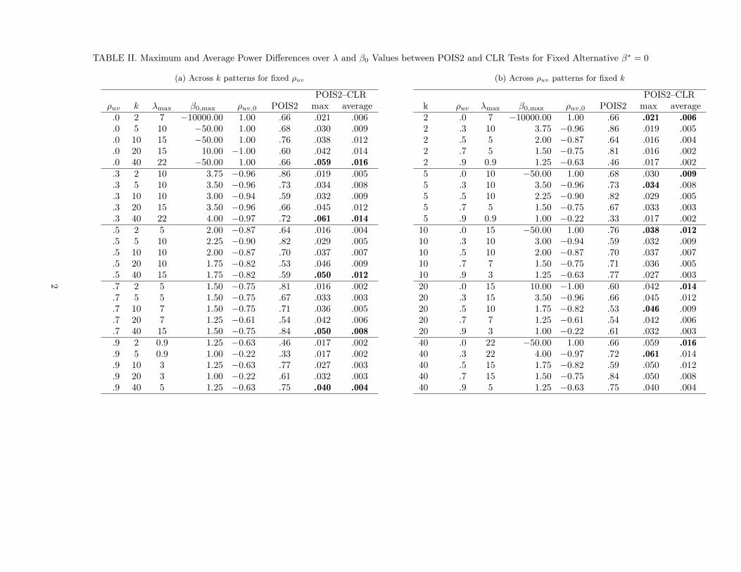
the POIS2 and CLR tests for �nite �0 values, rather than PD�s as �0 ! �1: Speci�cally, TableII reports maximum and average PD�s over �0 2 R and � > 0 for a �xed true value �� = 0 for a
range of values of (�uv; k): As above, the choice of �� = 0 (and !21 = !22 = 1) is wlog. These PD�s
are equivalent to false coverage probability di¤erences (FCPD�s) between the CLR and POIS2 CS�s
for a �xed true value �� at incorrect values �0: They are necessarily nonnegative.
The � values considered are 1; 3; 5; 7; 10; 15; 20; as well as 22; 25 when k = 20 and 40; and :7; :8; :9
when k = 2 and 5 and �uv = :9: The positive and negative �0 values considered are those with
j�0j 2 f:25; :5; :::; 3:75; 4; 5; 7:5; 10; 50; 100; 1000; 10000g: These (�; �0) values were chosen, based onpreliminary simulations, to ensure that changes in the PD�s in Table II (and Tables III and IV
below) across neighboring values (�; �0) are small.
The number of simulation repetitions employed is 5; 000: The critical values are determined
using 100; 000 simulation repetitions. For example, the simulation standard deviations for the PD�s
for (�uv; k) = (0; 20) and any �xed (�0; �) value range from [:0013; :0040] across di¤erent (�0; �)
values, which compares to simulated averages of the PD�s over (�0; �) values that are of the :014
order of magnitude.
Tables II(a) and II(b) contain the same numbers, but are reported di¤erently to make the
patterns in the table more clear. Table II(a) shows variation across k for �xed �uv; whereas Table
II(b) shows variation across �uv for �xed k: The third and fourth columns in each table report the
values of � and �0 at which the maximum PD is obtained. The �fth column in each table reports
21
�uv;0; which is the correlation between the structural-equation and reduced-form errors when �0
is the true value (based on the assumption that the consistently-estimable reduced-form variance
matrix is the same whether the truth is �0 or ��): In contrast, �uv is the same correlation, but
when �� is the true value� which is the true � value in the PD simulations. The sixth column in
the tables reports the power of the CLR test at the (�0; �) values that maximize the PD for given
(�uv; k); i.e., at (�0;max; �max):
Table II shows that the maximum (over (�0; �)) PD�s between the POIS2 and CLR tests range
between [:016; :061] over the (�uv; k) values. On the other hand, the average (over (�0; �)) PD�s
only range between [:002; :016] over the (�uv; k) values. This indicates that, although there are
some (�0; �) values at which the CLR test is noticeably o¤ the two-sided AE power envelope, on
average the CLR test�s power is not far from the power envelope.
In contrast, the analogous maximum and average PD ranges for the AR test are [:079; :513]
and [:012; :179]; see Table SM-III in the SM. For the LM test, they are [:242; :784] and [:010; :203];
see Table SM-IV in the SM. Hence, the power of AR and LM tests is very much farther from the
POIS2 power envelope than is the power of the CLR test.
Table II(a) shows that the maximum and average (over (�0; �)) PD�s for the CLR test are
clearly increasing in k: Table II(a) shows that for �uv � :3; the PD�s are maximized at more or less
the same �0 regardless of the value of k: For �uv = 0; this is also true to a certain extent, because
the sign of �0 is irrelevant (when �uv = 0) and the values 50 and 10; 000 are both large values.
Table II(a) also shows that for each �uv; the PD�s are maximized at � values that (weakly) increase
with k: The increase is particularly evident going from k = 20 to 40:
Table II(b) shows that for k � 5; the maximum PD�s are more or less the same for �uv � :7;
but noticeably lower for �uv = :9: For k = 2; the maximum PD�s are more or less the same for all
�uv considered. Table II(b) shows that, for each k; the PD�s are maximized at j�0j values that arecloser to 0 as �uv increases. Table II(b) also shows that, for each k; the PD�s are maximized at �
values that are closer to 0 as �uv increases.9
In sum, the maximum PD�s over (�0; �) are found to increase in k ceteris paribus and decrease
in �uv ceteris paribus. The � values at which the maxima are obtained are found to (weakly)
increase with k ceteris paribus and decrease in �uv ceteris paribus. The j�0j values at which themaxima are obtained are found to be independent of k ceteris paribus and decrease in �uv ceteris
paribus.
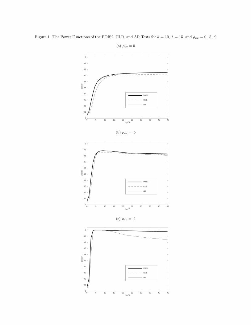
Next, Figure 1 provides a picture of how the power of the CLR, AR, and POIS2 tests di¤er
as a function of �0 when other parameters are held �xed. Results given are for three parameter
9See Table SM-II in the SM for how the maximum PD�s over �0 vary with � for the (�uv; k) values in Table II.
22
con�gurations �uv = 0; :5; :9 with � = 15; k = 10; and �� = 0 in all three con�gurations. These
parameter con�guations are chosen because they are ones in which the power of the CLR test is
noticeably o¤ the power envelope for su¢ ciently large �0 when �uv = 0 and :5:
Figure 1(a) for �uv = 0 shows: (i) the power of all three tests does not go to one as �0 ! 1(the limit value depends on the magnitude of �; which is 15 in Figure 1), (ii) the CLR test is o¤
the power envelope and the AR test is on the power envelope (up to the numerical accuracy) for
large �0 � ��; and (iii) the reverse is true for smaller �0 � ��:Figures 1(b) for �uv = :5 shows: (i) the power of all three tests does not go to one as �0 !1;
(ii) the CLR test is o¤ the power envelope for large �0 � �� and on the power envelope (up to thenumerical accuracy) for smaller �0 � ��; and (iii) the AR test is on the power envelope (up to thenumerical accuracy) for intermediate values of �0 � �� and o¤ the power envelope for larger and
smaller �0 � ��:Figures 1(c) for �uv = :9 shows: (i) the power of all three tests does not go to one as �0 !1;
but the powers of the CLR and POIS2 tests are quite close to one for �0 large, (ii) the CLR test
is on the POIS2 power envelope (up to the numerical accuracy) for all �0 values, and (iii) the AR
test is o¤ the POIS2 power envelope for most of the �0 values considered, including small and large
�0 values.
In all of the simulations considered (across the parameters scenarios considered in Table II), the
CLR test was found to be on the POIS2 power envelope (up to the numerical accuracy) for small
values of �0 � ��:The numerical results in this section show that the �nding of AMS that the CLR test is essen-
tially on the two-sided AE power envelope does not hold when one considers a broader range of null
and alternative hypothesis values (�0; ��) than those considered in the numerical results in AMS.
10 Di¤erences between CLR Power and an Average Over �
Power Envelope
In this section, we introduce a �WAP2�power envelope for similar tests with weight functions
over: (i) a �nite grid of � values, f�j > 0 : j � Jg; (ii) the same two-points (��; �j) and (�2�; �2j)as in AMS for each �j for j � J; and (iii) the same uniform weight function over ��=jj��jj as inCHJ. In particular, we use the uniform weight function over the 36 values of � in f2:5; 5:0; :::; 90:0g:
The WAP2 envelope is a function of (�0; ��): The WAP2(Q; �0; ��) test statistic that generates
this envelope is of the formPJj=1( (Q;�0; ��j ; �j)+ (Q;�0; �2�j ; �2j))=
PJj=1 2 2(QT ;�0; ��; �j);
where the functions (Q;�0; �; �) and 2(QT ;�0; �; �) are as in AMS (and as in (12.5) in the SM).
23
The WAP2(Q; �0; ��) conditional critical value �2;�0;J(qT ) is de�ned to satisfy PQ1jQT (WAP2(Q;
�0; ��) > �2;�0;J(qT )jqT ) = � for all qT � 0; where PQ1jQT (�jqT ) denotes probability under thedensity fQ1jQT (�jqT ); which is speci�ed in (12.3) in the SM.
To be consistent with Tables I and II, we report PD�s between the WAP2(Q; �0; ��) and CLR
tests for �� = 0 and a range of �0 values. These PD�s are equivalent to the FCPD�s between
the CLR and WAP2 CS�s for �xed true �� and varying incorrect �0 values. The di¤erences are
necessarily nonnegative.
We consider �uv 2 f0; :3; :5; :7; :9; :95; :99g; k = 2; 5; 10; 20; 40; the same �0 values as in Table
II, and !21 = !22 = 1: (The large �uv values of :95 and :99 are included to show that the results are
not sensitive to �uv being close to one.) Since �� = 0; � = �uv: Section 22 in the SM shows that
taking �� = 0 and !21 = !22 = 1 is wlog provided the support of the weight function for � is scaled
by !22 when !2 6= 1: The number of simulation repetitions employed is 1; 000 for each �j value.
With power averaged over the 36 �j values and independence of the simulation draws across �j ;
this yields simulation SD�s that are comparable to using 36; 000 simulation repetitions. The critical
values are determined using 100; 000 simulation repetitions for k = 5 and 10; 000 for other values
of k:
For brevity, Table III reports results only for k = 5 for a subset of the �0 values considered.
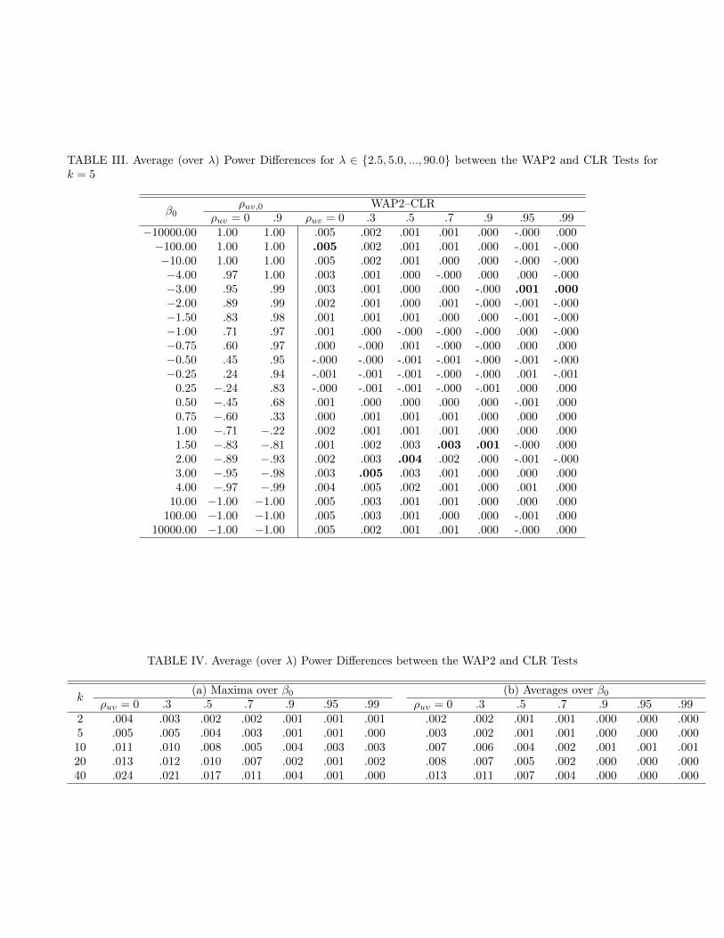
Results for all values of k and �0 considered are given in Table SM-V in the SM. Table IV reports
summary results for all values of k: In particular, Table IV(a) provides the maxima over �0 of the
average over � PD�s for each (�uv; k): Table IV(b) provides the average over �0 of the average over
� PD�s for each (�uv; k):
Table III shows that the CLR test has power quite close to the WAP2 power envelope for k = 5:
The PD�s for �uv 2 f0; :3; :5; :7g; we have PD2 [:000; :005] and SD2 [:0003; :0007] across all �0values. For �uv 2 f:9; :95; :99g; we have PD2 [:000; :001] and SD2 [:0000; :0003] across all �0 values.
Table IV shows that PD�s between the WAP2 power envelope and the CLR power are increasing
in k and decreasing in j�uvj: For k = 2; the maximum PD over �0 and �uv values is very small:
:004: In the worst case for CLR, which is when (k; �uv) = (40; 0); the maximum PD over �0 values
is substantially larger: :024: The average (over �0 values) PD in this case is :013; which is not very
large. For k = 40 and �uv � :9; the maximum PD (over �0 and �uv values) is very small: :004: This
is consistent with the theoretical optimality properties of the CLR test as �uv ! �1 described inSection 8. For k = 40 and �uv � :9; the average PD (over �0 values and the �ve �uv values) is very
small: :000: The second worst case for CLR in Table IV is when (k; �uv) = (20; 0): In this case, the
maximum PD over �0 values is :013; which is noticeably lower than :024 for (k; �uv) = (40; 0):
In conclusion, the results in Tables III and IV show that the CLR test is very close to the WAP2
24
power envelope for most (k; �uv; �0) values, but can deviate from it by as much as :024 for some �0
values when (k; �uv) = (40; 0):
25
References
Anderson, T. W. (1946): �The Non-central Wishart Distribution and Certain Problems of Multi-
variate Statistics,�Annals of Mathematical Statistics, 17, 409-431.
Anderson, T. W. and H. Rubin (1949): �Estimation of the Parameters of a Single Equation in a
Complete System of Stochastic Equations,�Annals of Mathematical Statistics, 20, 46�63.
Andrews, D. W. K. (1998): �Hypothesis Testing with a Restricted Parameter Space,�Journal of
Econometrics, 84, 155�199.
Andrews, D. W. K., and P. Guggenberger (2015): �Identi�cation- and Singularity-Robust Infer-
ence for Moment Condition Models,�Cowles Foundation Discussion Paper No. 1978, Yale
University.
� � � (2016): �Asymptotic Size of Kleibergen�s LM and Conditional LR Tests for Moment Con-
dition Models,�Econometric Theory, 32, forthcoming. Also available as Cowles Foundation
Discussion Paper No. 1977, Yale University.
Andrews, D. W. K., M. J. Moreira, and J. H. Stock (2004): �Optimal Invariant Similar Tests for
Instrumental Variables Regression with Weak Instruments,�Cowles Foundation Discussion
Paper No. 1476, Yale University.
� � � (2006): �Optimal Two-sided Invariant Similar Tests for Instrumental Variables Regres-
sion,�Econometrica, 74, 715�752.
Andrews, D. W. K. and W. Ploberger (1994): �Optimal Tests When a Nuisance Parameter Is
Present Only Under the Alternative,�Econometrica, 63, 1383�1414.
Chamberlain, G. (2007): �Decision Theory Applied to an Instrumental Variables Model,�Econo-
metrica, 75, 609�652.
Chernozhukov, V., C. Hansen, and M. Jansson (2009): �Admissible Invariant Similar Tests for
Davidson, R. and J. G. MacKinnon (2008): �Bootstrap Inference in a Linear Equation Estimated
by Instrumental Variables,�Econometrics Journal, 11, 443�477.
Dufour, J.-M. (1997): �Some Impossibility Theorems in Econometrics with Applications to Struc-
tural and Dynamic Models,�Econometrica, 65, 1365�1387.
26
Dufour J.-M., and M. Taamouti (2005): �Projection-Based Statistical Inference in Linear Struc-
tural Models with Possibly Weak Instruments,�Econometrica, 73, 1351�1365.
Elliott, G., U. K. Müller, and M. W. Watson (2015): �Nearly Optimal Tests When a Nuisance
Parameter Is Present Under the Null Hypothesis,�Econometrica, 83, 771�811.
Hillier, G. H. (1984): �Hypothesis Testing in a Structural Equation: Part I, Reduced Form Equiv-
alence and Invariant Test Procedures,�unpublished manuscript, Dept. of Econometrics and
Operations Research, Monash University.
� � (2009): �Exact Properties of the Conditional Likelihood Ratio Test in an IV Regression
Model,�Econometric Theory, 25, 915�957.
Kleibergen, F. (2002): �Pivotal Statistics for Testing Structural Parameters in Instrumental Vari-
ables Regression,�Econometrica, 70, 1781-1803.
Mikusheva, A. (2010): �Robust Con�dence Sets in the Presence of Weak Instruments,�Journal
of Econometrics, 157, 236�247.
Mills, B., M. J. Moreira, and L. P. Vilela (2014): �Tests Based on t-Statistics for IV Regression
with Weak Instruments,�Journal of Econometrics, 182, 351�363.
Moreira, M. J. (2003): �A Conditional Likelihood Ratio Test for Structural Models,�Economet-
rica, 71, 1027-1048.
� � � (2009): �Tests with Correct Size When Instruments Can Be Arbitrarily Weak, Journal of
Econometrics, 152, 131�140.
Moreira, H. and M. J. Moreira (2013): �Contributions to the Theory of Optimal Tests,�unpub-
lished manuscript, FGV/EPGE, Brasil.
Moreira, M. J. and G. Ridder (2017): �Optimal Invariant Tests in an Instrumental Variables Re-
gression with Heteroskedastic and Autocorrelated Errors,�manuscript in preparation, FGV,
Brazil.
van der Vaart, A. W. (1998): Asymptotic Statistics. Cambridge, UK: Cambridge University Press.
van der Vaart, A. W. and J. A. Wellner (1996): Weak Convergence and Empirical Processes. New
York: Springer.
27
Wald, A. (1943): �Tests of Statistical Hypotheses Concerning Several Parameters When the Num-
ber of Observations Is Large,�Transactions of the American Mathematical Society, 54, 426�
482.
28
TABLE I. Differences in Probabilities of Infinite-Length CI’s for the CLR and POIS2∞ CI’s, and Probabilities ofInfinite-Length POIS2∞ CI’s as Functions of k, λ and ρuv