On Parameter Estimation - Applications in Radio Astronomy ...837951/FULLTEXT01.pdf · On Parameter...

On Parameter Estimation -Applications in Radio

Astronomy and Power Networks

Jonas Lundback

Ronneby, May 2005

Department of Telecommunications and Signal Processing

Blekinge Institute of Technology

S-372 25 Ronneby, Sweden

c© Jonas Lundback

Blekinge Institute of TechnologyLicentiate Series No. 2005:09

ISSN 1650-2140ISBN 91-7295-065-X

Published 2005Printed by Kaserntryckeriet ABKarlskrona 2005Sweden

v

Abstract

Signal processing is a common part of the modern society used to obtainhigh functionality in a vast number of applications. As the development ofadvanced electronics and powerful computers continue, the limit of the func-tionality in many systems is increased. Furthermore, as the signal processingcan be performed on digitalized signals more advanced methods and algo-rithms can be employed and enhance the results.

In radio-based astronomy a new window of discovery against space hasopened using digitally based antenna array systems to observe signals withspectral contents ranging up to a major part of the VHF-band. This enables ahigh degree of flexibility and incorporates several areas e.g. radio astronomy,signal processing and advanced electronic design, in the development andconstruction of the technology. The usage of digital signal processing is alsoseen in power networks to control and monitor the state of the system. Thepower network is a complex and vital construction for the population thatdemand a high degree of security and reliability. Methods for monitoringand diagnostics are needed. If a fault can be found with high accuracy thetime spent on repairs can be kept low reducing the cost and the consumersdiscontent.

This thesis concerns parameter estimation within radio-based astronomyand fault localization on power lines. In this thesis the connection betweenthe two areas is the use of electromagnetic modelling of underlying physicalproperties, parameter estimation and digitally based equipment used for ad-vanced signal processing. The first area concerns the estimation of propertiesof electromagnetic waves e.g. direction of arrival and state of polarization,using an antenna array consisting of Tripole antennas. The properties of thisantenna and the corresponding array configuration are investigated in partI-III of this thesis. The second area concerns fault localization on power linesusing frequency modulated radar techniques. Part IV and V of this thesispresent the concept and properties of this fault locator.

vii

Preface

Part

I On Signal Separation Using Polarization Diversity and Tripole Arrays

II Analysis of a Tripole Array for Polarization and Direction of ArrivalEstimation

III Fundamental Limitations for Polarization Estimation with Applicationsin Array Processing

IV On Fault Localization on Power Lines - An FMCW Based Fault Locator

V FMCW Radar for Fault Localization on Power Lines

ix

Acknowledgments

I would like to express my profound gratitude to Professor Sven Nordebowho has been my advisor and guide throughout the work of this thesis. Hehas generously shared his knowledge and experience in the field of signalprocessing. I am utterly grateful for the wisdom and experience, rangingfrom Radio astronomy to Rock’n Roll, that Professor Bo Thide has conveyedduring our work in the LOIS project.

Furthermore, I want to seize the opportunity to thank the following peoplefor their involvement in my work; the staff at AerotechTelub, especially IngeFalk and Hakan Petersson, for their helpfulness and support towards the LOISproject. Christer Stoij at Sivers IMA for generously supplying equipment andtechnical knowledge of microwave engineering. Magnus Akke at ABB andLund Institute of Technology for sharing his knowledge in power engineeringand the arrangement of measurement equipment.

I wish to thank my colleagues at the department of electronics, especiallymy roommate Therese Sjoden, and the colleagues at the school of Mathematicsand System Engineering. For the interesting discussions, the collaborationsand the continuous education I am truly thankful.

During this period of my graduate education I have had the fortune ofmeeting many people that have affected my work and increased my knowledgeand experience. I hope that none of them are feeling forgotten when readingthis.

I thank my family and parents-in-law for their support and encouragementthat are important ingredients in this work, and a special thanks to Kjell forhis endless supply of convenient comments.

Finally, I am deeply thankful for all the love, support and patience that myfiancee Jessica has generously offered me, even in times where I might havedeserved less. She is truly remarkable and a most wonderful kind-heartedwoman.

Jonas LundbackVaxjo, May 2005

xi

Contents

Publication list . . . . . . . . . . . . . . . . . . . . . . . . . . . . . . . . . . . . . . . . . . . . . . . . . . . . . . 13

Introduction . . . . . . . . . . . . . . . . . . . . . . . . . . . . . . . . . . . . . . . . . . . . . . . . . . . . . . . . . 15

Part

I On Signal Separation Using Polarization Diversity and Tripole Arrays. . . . . . . . . . . . . . . . . . . . . . . . . . . . . . . . . . . . . . . . . . . . . . . . . . . . . . . . . . . . . . . . . . . 27

II Analysis of a Tripole Array for Polarization and Direction of ArrivalEstimation . . . . . . . . . . . . . . . . . . . . . . . . . . . . . . . . . . . . . . . . . . . . . . . . . . . . . . . . 41

III Fundamental Limitations for Polarization Estimation with Applicationsin Array Processing. . . . . . . . . . . . . . . . . . . . . . . . . . . . . . . . . . . . . . . . . . . . . . . . 56

IV On Fault Localization on Power Lines - An FMCW Based Fault Locator.. . . . . . . . . . . . . . . . . . . . . . . . . . . . . . . . . . . . . . . . . . . . . . . . . . . . . . . . . . . . . . . . . . . 74

V FMCW Radar for Fault Localization on Power Lines . . . . . . . . . . . . . 121

13

Publication list

Part I is published as:

J. Lundback, S. Nordebo, ”On Signal Separation Using Polarization Diversityand Tripole Arrays”, In Proc. Mathematical Modelling of Wave Phenomena,Vaxjo, Sweden, November 2002.

This work has also been published in revised form as:J. Lundback, S. Nordebo, ”On Polarization Estimation Using Tripole Arrays”,In Proc. IEEE Antennas and Propagation 2003, Columbus, USA, July 2003.

Part II is published as:

J. Lundback, S. Nordebo, ”Analysis of a Tripole Array for Polarization andDirection of Arrival Estimation”, In Proc. Third IEEE Sensor Array andMultichannel Signal Processing Workshop, Sitges, Spain, July 2004.

Part III is submitted as:

S. Nordebo, M. Gustavsson, J. Lundback, ”Fundamental Limitations for Po-larization Estimation with Applications in Array Processing”, submitted toIEEE Transactions on Signal Processing.

Part IV is published as:

J. Lundback, S. Nordebo, M. Akke, T. Biro, ”On Fault Localization on PowerLines - An FMCW Based Fault Locator”, Research Report 05030, ISSN 1650-2647, VXU/MSI/EL/R/–05030/–SE, Vaxjo university, April 2005.

Part V is accepted for presentation as:

J. Lundback, S. Nordebo, ”FMCW Radar for Fault Localization on PowerLines”, accepted for presentation at RVK05, Linkoping, Sweden, June 2005.

14

15

Introduction

The work summarized in this thesis can be divided into two parts connected bythe use of electromagnetic modelling in signal processing applications, specif-ically parameter estimation. This introduction is divided into two parts; thefirst part introduces the concept of the Tripole antenna and the related vectorsensor. The second part introduces the area of fault localization on powerlines.

The Tripole Antenna and the Related Vector-sensor

In [Com81] Compton introduces the concept of the Tripole antenna which isan antenna constructed by three perpendicular dipoles centred at the sameposition. This can be interpreted as an antenna array with three dipole anten-nas and in [Com81] the Tripole is shown to possess good interference rejectionproperties and polarization separation properties when adaptive tracking isutilized.

To fully exploit and measure the properties of an electromagnetic waveNehorai and Paldi in [NP94] introduced the vector-sensor that consists ofsix electric and magnetic elements, collocated in space but orthogonally ori-ented. This enables measurements of the complete electromagnetic field at theantenna, which could not be accomplished using scalar sensors. The vector-sensor provides more flexibilities and robustness compared with the Tripoleantenna. Specifically, the vector-sensor can possess a good performance in asituation where the Tripole antenna is less efficient [NP94]. These benefits areobtained at a cost of the three additional magnetic dipole elements and corre-sponding additional receiver equipment, increased computational complexityand mutual coupling between the electrical dipoles and the magnetic dipoles.The choice of antenna is therefore not obvious.

In light of the benefit of measuring the complete electromagnetic field thevector-sensor has been investigated and proposed as an efficient antenna dur-ing the last decade, see e.g. [HN96, KCTN96a, KCTN96b, ANT99, HN95,Li93]. In the context of Direction-Of-Arrival (DOA) and polarization esti-mation there are several publications concerning the usage of eigenstructurebased methods e.g. ESPRIT [Tre02] and MUSIC [PS97] or methods devel-oped based on their foundations, see e.g. [Li93, HTN99, WZ00] and referencestherein.

In radio-based astronomy the search-space of incoming electromagneticwaves can be limited to the upper hemisphere and thereby the number of

16

elements can be reduced, [JTR04, Won01], and still provide information aboute.g. the source location for an arbitrarily polarized electromagnetic wave.

Within the digital-radio-telescope project LOIS [Loi05], related to the LO-FAR project [Lof05], the Tripole antenna has to this day been the proposedantenna configuration based on its simple but effective structure. However,the possibility of using other or similar advanced antennas is under consider-ation. Since the number of antennas in this digital-radio astronomy projectis planned to be large the choice of the antenna type is important. Froma cost-effective and flexibility/robustness point of view the Tripole antennais suitable for this application where the antenna array, in the fully func-tional stage, should be able to measure incoming electromagnetic waves withfrequencies ranging up to approximately 200 MHz.

Each antenna, regardless of configuration, is connected to an individualdigital-receiver capable of guaranteeing 10 dB signal-to-noise ratio at −103dBm input power with a 3.4 kHz bandwidth at 5 MHz. The receiver is com-pletely based on digital processing and controlled by central unit, e.g. a digi-tal signal processor or a field programmable gate array capable of supplyingthe user with a large flexibility depending on the requirements of operation.Communication with the receivers in the array is made over the Internet andeffectively moves the computational burden to a central computer, an ordi-nary desktop computer or a distributed parallel processing unit. This enablesthe usage of advanced digital signal processing algorithms.

The work done on the Tripole array is summarised below and included aspart I-III of this thesis.

Fault Localization on Power Lines

The modern society demands a robust and reliable power system that canguarantee continuous power delivery for the major part of the year. Sincepower systems are large and complex constructions there is a need for fastand accurate fault localization equipment.

A major threat against technology such as a power network is solar windscontaining large amounts of energy in clouds of charged plasma originatedfrom e.g. coronal mass ejections (CMEs). Although the earth magnetic fieldis protective, a high-energy event can effectively disable a power network. Onescientific goal of the LOIS project [Loi05] is to monitor the sun and the spaceweather, to provide accurate reports and warnings concerning high-energysolar events that approaches the earth. Using the information gathered aboutthe event, the concerned parties can secure the continuous operation.

17

The fact that researchers have investigated the topics of fault locators forseveral years displays the need for accurate and economic solutions. With theaid of such equipment, faults can be accurately localized and repair crews canmaximise their efficiency regarding the time spent finding the fault location.Since a general power network can include a vast number of components andcircuits, different voltage levels, different feeder configurations and differenttypes of cables with different length etc., it is not an obvious task to constructa general fault locator, see e.g. [And95, And98].

Proposed fault locators are based on e.g. travelling waves generated by thefault, external signal injection techniques, algorithms using voltage and cur-rent phasors and measurements of the voltage and the currents on the powerline. The phasor based fault locators are in general mounted within the powersystem and measures the post-fault transients to acquire the correspondingfundamental frequency phasors, either by filtering or by numerical methods[LER85]. This approach is similar to the fault locators based on raw voltageand current measurements but here the analysis to obtain the fault locationis performed in the time domain, see e.g. [AGH00, BG04].

Travelling wave based fault locators are often considered to be mountedwithin the power system and in conjunction with the Global Position Systemthe travelling waves are time-stamped at both ends of the power line. Usingknowledge of the power line under investigation the distance to the faultcan be estimated. This requires some form of communication between thefault locators to obtain the difference in the time of arrival of the travellingwave at both ends, see e.g. [ZXX04, Lee93]. The travelling waves producean electromagnetic field transmitted by the power cable that could provideinformation about the fault and be measured using e.g. a polarization sensitiveantenna, such as the Tripole antenna.

Signal injection techniques can be used both on an energized and on adeenergized power line since the transients and travelling waves generatedby the fault are not of primary interest. This type of fault locator is basedon Time Domain Reflectometry where the reflection of the injected signalat an impedance discontinuity is recorded and processed to obtain a timedifference between the time of transmission and the time of arrival. There aredifferent types of signals or waveforms suggested for usage, see e.g. [TF96] andreferences therein, but the most common is pulse-shaped signals. Dependingon the desired resolution or accuracy and the maximum distance to a fault,there exist a flexibility in selecting the signal properties.

In [DST72] the authors suggested the usage of Frequency Modulated Con-tinuous Wave (FMCW) signals instead of the pulse-shaped signals. The

18 Introduction

FMCW radar is a well-known and versatile technique in the radar community,see e.g. [Gri90, Sto92, Sko80]. It has interesting properties that are of greatimportance in the context of fault localization on power lines e.g. the time-bandwidth product can be selected large resulting in good accuracy, severalsynchronised measurement can be averaged to obtain better signal-to-noiseratio and the post-measurement analysis can be performed in the frequencydomain. This concept has not been explored further and in this thesis wecontinue to develop and investigate the concept in a situation involving a oneline to ground (1LG) fault. The work done regarding fault localization issummarised below and included as part IV-V of this thesis.

Part I - On Signal Separation Using PolarizationDiversity and Tripole Arrays

This paper investigates the linear independency of the steering vectors asso-ciated with an array of Tripole antennas. There is a clear connection betweenthese properties and the estimation quality using high-resolution subspacebased methods such as e.g. MUSIC. We state conditions based on the num-ber of incoming signals and their polarization state and develope bounds onthe number of linearly independent steering vectors one can expect if theconditions are fulfiled. Simulations are included to exemplify the theory.

Part II - Analysis of a Tripole Array for Polar-ization and Direction of Arrival Estimation

We consider using the tripole array to estimate the polarization state andone-dimensional DOA of one incoming electromagnetic wave. The quality ofthe estimates are investigated based on the Cramer-Rao Bound. Assumingknowledge about the direction of arrival of the incoming wave, using beam-forming or a priori information, we introduce a polarization state estimatorbased on the stokes parameters and a linear Least-Square formulation. Theperformance of the estimator is compared to Cramer-Rao Bound and is seento indicate good estimation possibilites.

Introduction 19

Part III - Fundamental Limitations for Polar-ization Estimation with Applications in ArrayProcessing

This paper investigates fundamental physical limits concerning polarizationestimation using electrically small antennas. The modelling of the receivingantennas is based on spherical vector modes, radiating Q and broadband Fanotheory. The concept of a probing multimode array utilizing beamforming tosuppress interferers is introduced. A maximum likelihood polarization esti-mator for the probing array is derived. The Fisher Information is used as ameasure of the performance of the multimode array for polarization estima-tion. It is seen that the performance is invariant to the direction parametersand the polarization state but depends strongly on the degree of polarization,the electrical size of the antenna and the system bandwidth.

Part IV - On Fault Localization on Power Lines- An FMCW Based Fault Locator

In this report we investigate the use of FMCW radar for fault localizationon power lines. This includes basic theory and an electromagnetic model forthe frequency dependent transmission line parameters. Simulations and cal-culations of the corresponding theoretical optimum performance obtained viathe Cramer-Rao Bound are included. Also, we present and discuss measure-ments made in laboratory and in a field-experiment of an FMCW based faultlocator.

Part V - FMCW Radar for Fault Localizationon Power Lines

This paper summarizes the work made concerning fault localization on powerlines. The concept of an FMCW based fault locator is presented using trans-mission line theory and the performance is quantified using the Cramer-RaoBound. Measurements and simulations are included and processed using high-resolution spectrum estimation methods.

20 Introduction

Bibliography

[AGH00] S. M. McKennaa A. Gopalakrishanan, M.Kezunovic and D.M.Hamai. Fault location using the distributed parameter trans-mission line model. IEEE Transactions on Power Delivery,15(4):1169–1174, October 2000.

[And95] P. M. Anderson. Analysis of Faulted Power Systems. Wiley-IEEEPress, 1995.

[And98] P. M. Anderson. Power System Protection. Wiley-IEEE Press,1998.

[ANT99] K. C. Ho A. Nehorai and B. T. G. Tan. Minimum-noise-variancebeamformer with an electromagnetic vetor-sensor. IEEE Trans-actions on Signal Processing, 47(3):601–618, March 1999.

[BG04] S. M. Brahma and A. A. Girgis. Fault location on a transmissionline using synchronized voltage measurements. IEEE Transac-tions on power Delivery, 19(4):1619–1622, October 2004.

[Com81] R. T. Compton. The tripole antenna: An adaptive array withfull polarization flexibility. IEEE Trans. Antennas Propagat.,29(6):944–952, November 1981.

[DST72] W. Pomeroya D. Stevens, G. Ott and J. Tudor. Frequency–modulated fault locator for power lines. IEEE Transactions onPower Apparatus and Systems, 95(5):1760–1768, 1972.

[Gri90] H. D. Griffiths. New ideas in fm radar. Electronics & Commu-nication Engineering Journal, 2(5):185–194, October 1990.

21

22 Introduction

[HN95] B. Hochwald and A. Nehorai. Polarimetric modeling and param-eter estimation with applications to remote sensing. IEEE Trans.Signal Processing, 43(8):1923–1935, August 1995.

[HN96] B. Hochwald and A. Nehorai. Identifiability in array processingmodels with vector-sensor applications. IEEE Transactions onSignal Processing, 44:83–95, January 1996.

[HTN99] K-C Ho, K-C Tan, and A. Nehorai. Estimating directions ofarrival of completely and incompletely polarized signals withelectromagnetic vector sensors. IEEE Trans. Signal Processing,47(10):2845–2852, October 1999.

[JTR04] R. Shavit J. Tabrikian and D. Rahamim. An efficient vector sen-sor configuration for source localization. IEEE Signal ProcessingLetters, 11(8):690–693, August 2004.

[KCTN96a] K. C. Ho K. C. Tan and A. Nehorai. Linear dependence of steer-ing vectors of an electromagnetic vector-sensor. IEEE Transac-tions on Signal Processing, 44:3099–3107, December 1996.

[KCTN96b] K. C. Ho K. C. Tan and A. Nehorai. Uniqueness study ofmeasurements obtainable with arrays of electromagnetic vector-sensors. IEEE Transactions on Signal Processing, 44:1036–1039,April 1996.

[Lee93] H. Lee. Development of an accurate traveling wave fault loca-tor using global positioning satelites. In Spring Meeting of theCanadian Electrical Association, Montreal, Quebec, March 1993.

[LER85] M. M. Saha L. Eriksson and G. D. Rockefeller. An accurate faultlocator with compensation for apparent reactance in the faultresistance resulting from remote-end infeed. IEEE Transactionson Power Apparatus and Systems, PAS-104(2):424–436, Febru-ary 1985.

[Li93] J. Li. Direction and polarization estimation using arrays withsmall loops and short dipoles. IEEE Trans. Antennas Propagat.,41(3):379–387, March 1993.

[Lof05] Low frequency array. Webpage, February 2005.http://www.lofar.org/.

Introduction 23

[Loi05] Lofar outrigger in scandinavia. Webpage, February 2005.http://www.lois-space.net.

[NP94] A. Nehorai and E. Paldi. Vector-sensor array processing for elec-tromagnetic source localization. IEEE Transactions on SignalProcessing, 42(2):376–398, February 1994.

[PS97] R. Moses P. Stoica. Introduction to Spectral Analysis. PrenticeHall, 1997.

[Sko80] Merrill I. Skolnik. Introduction to Radar Systems. McGraw-Hill,2 edition, 1980.

[Sto92] A. G. Stove. Linear fmcw radar techniques. IEE Proceedings–F,139(5):343–350, October 1992.

[TF96] V. Taylor and M. Faulkner. Line monitoring and fault locationusing spread spectrum on power line carrier. Generation, Trans-mission and Distribution, IEE, 143(5):427–434, 1996.

[Tre02] H. L. Van Trees. Optimum Array Processing. John Wiley & Sons,Inc., New York, 2002.

[Won01] K. T. Wong. Direction finding/polarization estimation – dipoleand/or loop triad(s). IEEE Transactions on Aerospace and Elec-tronic Systems, 37(2):679–684, April 2001.

[WZ00] K. T. Wong and M. D. Zoltowski. Closed–form direction findingand polarization estimation with arbitrarily spaced electromag-netic vector–sensors at unknown locations. IEEE Trans. Anten-nas Propagat., 48(5):671–681, May 2000.

[ZXX04] L. Zhengyi Z. Xiangjun, Li K. K. and Y. Xianggen. Fault locationusing traveling wave for power networks. In Industry ApplicationsConference, 2004. 39th IAS Annual Meeting, volume 4, pages2426–2429. IEEE, 2004.

Part I

On Signal SeparationUsing Polarization

Diversity and TripoleArrays

Part I is published as:

J. Lundback, S. Nordebo, ”On Signal Separation Using Polarization Diversityand Tripole Arrays”, In Proc. Mathematical Modelling of Wave Phenomena,Vaxjo, Sweden, November 2002.

On Signal Separation Using Polarization

Diversity and Tripole Arrays

J. Lundback, S. Nordebo

Abstract

This paper concerns signal separation in the context of estimatingthe Direction Of Arrival (DOA) and the state of the electromagneticpolarization using Tripole antenna arrays. We derive an analytical ex-pression for the electromagnetic far-field of the Tripole antenna arrayand a signal model for the waves received by the array. In a two–dimensional DOA–parameter space it is shown that there can be atmost two linearly independent steering vectors per distinct DOA. Moreover, steering vectors are linearly independent iff the polarization stateof the corresponding two signals are different. In the case of DOA froma one-dimensional parameter space we show that the steering vectorsare linearly independent if the Haar condition is satisfied and that thereare at most equal number of distinct DOA as there are Tripole antennaswith at most two distinct states of polarizations per DOA. This is illus-trated in simulations using MUSIC and Capons method for parameterestimation.

1 Introduction

The use of signal processing on antenna arrays that have certain physicalproperties enables the estimation of electromagnetic (EM) wave parameterssuch as the Direction Of Arrival (DOA) and the state of polarization, seee.g. [Li93, WZ00, HTT98]. Related problems of great technical relevance aresignal separation and interference cancellation based on space and polarizationdiversity, see e.g. [WZ00, HTT98, Com81].

Within classical estimation theory using subspace methods such as e.g.Multiple Signal Classification (MUSIC) [WZ00, HTT98, SV93] it is usuallyimplicitly assumed that a steering vector corresponds to the sought param-eter (such as DOA) if this steering vector belongs to the signal subspace.

27

28 Part I

This is usually true for a simple array problem, such as with the UniformLinear Array (ULA) and a one–dimensional parameter space, if the Haar con-dition is satisfied [Kre78]. For multi–dimensional parameter estimation suchas with (2–D) polarization and (2–D) DOA estimation the situation is muchmore complicated. It is possible that a steering vector is linearly dependentof the associated signal subspace even though this steering vector does notcorrespond to any present signal [HTT98]. This uniqueness issue is of greatimportance for the possibilities of DOA and polarization estimation as wellas for the possibilities of signal separation and interference cancellation.

In this contribution we study the array of Tripole antennas and the prop-erties of the associated array manifold given a certain antenna length andpropagation constant. We show that there are no more than two linearly in-dependent steering vectors for each direction of arrival (DOA) and that thesesteering vectors are linearly independent iff they correspond to distinct statesof polarization. Hence, in principle, it is possible to estimate the state of po-larization of only one signal per DOA. Furthermore, in the case of a uniformlinear array and a one–dimensional DOA–parameter space (two–dimensionalwave propagation) we use the Haar condition to show that a steering vectoris linearly independent of the signal subspace if there are less distinct DOAsthen there are Tripole antennas. Hence, given M Tripole antennas, we areguaranteed to uniquely estimate M −1 distinct (1–D) DOAs regardless of thenumber of incoming signals and their state of polarization.

2 The Steering Vector Based Signal Model

The Tripole antennas are oriented so that the three antenna elements of length2h are aligned along the Cartesian base vectors x1, x2, x3, respectively. Themagnetic vector potential for antenna i = 1, 2, 3 is given by Ai(r) = Ai(r)xiwhere

Ai(r) =µ0

4π

∫ h

−h

Ii(xi)e−jk|r−xi

xi|

|r − xixi|dxi, (1)

cf. [Bal97], where µ0 is the permeability of free space, r = rr is the positionvector in spherical coordinates, Ii(xi) is the current distribution for antennai and k = ω/c = 2π/λ is the wave number for free space, ω the angularfrequency, λ the wave length and c the speed of wave propagation. We assumethat the current distribution is given by

Ii(xi) = I0i sin(β(h− |xi|)) (2)

On Signal Separation Using Polarization Diversity and Tripole Arrays 29

where β > k is the propagation constant for the antenna and I0i is the complexcurrent amplitude.

The electric far–field approximation for antenna i is given by the followingrelation, cf. [Bal97]

Ei(r) =e−jkr

krF i(r) = −jωAi(r) · (θθ + φφ) (3)

where F i(r) is the far–field amplitude and θ and φ the unit vectors for spher-ical angles. By inserting (1) and (2) in (3) we find the far–field amplitude forantenna i

F i(r) =−jkωµ0I0i

4πG(r · xi)xi · (θθ + φφ) (4)

where

G(ψ) =

∫ h

−h

sin(β(h− |x|))ejkψxdx = 2βcos(kψh) − cos(βh)

β2 − k2ψ2. (5)

It is assumed that β > k, and hence G(ψ) > 0 since |ψ| ≤ 1. Note also thatG(ψ) → βh2 when h→ 0.

Now, consider the situation where there are L waves impinging on theantenna array given by

El(r, t) = sl(t)(sin γlejηl θl + cos γlφl)e

jk

rl·r, l = 1, . . . , L (6)

where sl(t) is the complex baseband signal, γl and ηl are the two polarizationparameters interpreted as spherical angles on the poincare sphere cf. [Com81],

and rl, θl and φl are the unit spherical coordinate vectors corresponding tothe direction of the incoming wave front. The state of polarization of the lthwave is defined by the complex number Pl = tan γle

jηl .Suppose there are M Tripole antennas at positions rm, m=1,. . . ,M. The

lth received signal at antenna m and Tripole element i is proportional to thescalar product

El(rm, t)·F i(rl) ∼ ejk

rl·rmG(rl·xi)(xi·θlθl+xi·φlφl)·(sin γlejηl θl+cos γlφl) = ami

(7)cf. [SDS98], where the complex amplitudes ami are the elements of the steering

vector of the antenna array. Hence from (7), the 3M × 1 steering vector maybe written as

a(θl, φl, γl, ηl) = A(θl, φl)P(γl, ηl) (8)

30 Part I

where

A(θl, φl) = d(θl, φl) ⊗ (G(θl, φl)B(θl, φl)), (9)

d(θl, φl) = [ejk

rl·r1 · · · ejk

rl·rM ]T , (10)

G(θl, φl) = diag [G(rl · x1) G(rl · x2) G(rl · x3)] , (11)

B(θl, φl) =

x1 · θl x1 · φlx2 · θl x2 · φlx3 · θl x3 · φl

=

cos θl cosφl − sinφlcos θl sinφl cosφl− sin θl 0

, (12)

P(γl, ηl) =

(sin γl · e

jηl

cos γl

), (13)

and where ⊗ denotes the Kronecker product.The received signals at the antenna array can now be modelled as follows

x(t) = As(t) + n(t) (14)

where x(t) is the received 3M × 1 complex baseband signal, A = [a1 · · · aL]where al = a(θl, φl, γl, ηl), s(t) = [s1(t) · · · sL(t)]T and n(t) represents zeromean additive white Gaussian noise (AWGN) with covariance matrix σ2

nI.The range space of A is called the signal subspace.

3 Properties that guarantee linearly indepen-

dent steering vectors

In this section, we state five theorems that have great significance regardingthe uniqueness of DOA estimates using eigenspace methods such as MUSICand related techniques, see e.g. [WZ00, HTT98, SV93]. These theorems havealso a great impact on the possibilities to perform signal separation and in-terference cancellation, see e.g. [Com81].

Theorem 1 There are no more than two linearly independent steering vec-tors for any given DOA (θ, φ).

Proof: This follows directly from the vector space structure given in (8) wherethe matrix A(θ, φ) is 3M × 2. 2

Theorem 2 Given any fixed DOA (θ, φ). Two steering vectors a(θ, φ, γ, η)and a(θ, φ, γ′, η′) are linearly independent iff the corresponding states of po-larization are distinct, i.e. P = tan γejη 6= P ′ = tan γ′ejη

′

, or (γ, η) 6= (γ′, η′).


Proof: Since G(θ, φ) > 0 and B(θ, φ) has orthogonal columns, it followsthat C(θ, φ) = G(θ, φ)B(θ, φ) has full rank. Hence, A(θ, φ)x = d(θ, φ) ⊗C(θ, φ)x = 0 implies that x = 0 and the matrix A(θ, φ) has linearly indepen-dent columns. Now, since [a(θ, φ, γ, η) a(θ, φ, γ ′, η′)] = A(θ, φ)[P(γ, η) P(γ′, η′)]it is concluded that the two steering vectors a(θ, φ, γ, η) and a(θ, φ, γ ′, η′)are linearly independent iff det[P(γ, η) P(γ ′, η′)] 6= 0, or equivalently, P =tan γejη 6= P ′ = tan γ′ejη

′

. 2

The steering vectors belong to the complex vector space C3M . In general,the set of steering vectors a(θl, φl, γl, ηl)

L

l=1 may be linearly dependent, eventhough L < 3M and the points (θ1, φ1, γ1, η1) 6= · · · 6= (θL, φL, γL, ηL) aredistinct, cf. [HTT98]. We emphasize that this is a natural property sincethere is no Haar condition [Kre78] for functions of several variables.

In this contribution, we investigate sufficient conditions for linearly inde-pendent steering vectors when the array response vector d(θ, φ) satisfy theHaar condition. Specifically, we consider now the case with a uniform lineararray (ULA) with θ = π/2, 0 ≤ φ ≤ π, rm = x1(m − 1)λ/2 and d(φ) =d(π/2, φ) = [1 ejπ cosφ · · · ejπ cosφ(M−1)]T . The vector function d(φ) ∈ CM sodefined satisfies the Haar condition [Kre78], hence rank[d(φ1) · · ·d(φK)] = Kif K ≤ M and the points φ1 6= · · · 6= φK are distinct (cf. the Vandermondematrix).

Denote A(φ) = A(π/2, φ) and C(φ) = C(π/2, φ), hence A(φ) = d(φ) ⊗C(φ) and the corresponding steering vector is denoted a(φ, γ, η) = A(φ)P(γ, η).We are now ready to state the following theorem

Theorem 3 Suppose that the array response vector d(φ) ∈ CM satisfies theHaar condition. Then the matrix [A(φ1) · · ·A(φK)] has full rank if K ≤ Mand the points φ1 6= · · · 6= φK are distinct.

Proof: Consider the equation [A(φ1) · · ·A(φK)]x = 0, or d(φ1) ⊗ C(φ1)x1 +· · ·d(φK)⊗C(φK)xK = 0 where the right–hand side is a 3M × 1 zero vector.This equation can be rearranged as C(φ1)x1d

T (φ1)+ · · ·C(φK)xKdT (φK) =

0 where the right–hand side is a 3 ×M zero matrix. The last equation canbe written

[d(φ1) · · ·d(φK)]

xT1 C

T (φ1)...

xTKC

T (φK)

= 0

where the right–hand side is an M × 3 zero matrix. The Haar condition nowimplies that C(φk)xk = 0, and xk = 0 since C(φk) has full rank. Hence,x = 0 and the proof is concluded. 2

32 Part I

Finally, we state two theorems with direct application to eigenspace basedestimation techniques.

Theorem 4 Suppose that the array response vector d(φ) ∈ CM satisfies the

Haar condition. Given a set of steering vectors a(φl, γl, ηl)L

l=1 correspondingto K distinct DOA’s φ(k) where K ≤M −1. Then a steering vector a(φ, γ, η)

is linearly independent of the set a(φl, γl, ηl)L

l=1 if

1. φ 6= φl for all l = 1, . . . , L

2. φ = φl for just one index l ∈ 1, . . . , L and (γ, η) 6= (γl, ηl)

Proof: To prove the first statement above, assume that the vector a(φ, γ, η)

is linearly dependent of the set a(φl, γl, ηl)L

l=1, hence

a(φ, γ, η) +L∑

l=1

xla(φl, γl, ηl) = 0 (15)

where K ≤ M − 1 and φ 6= φl for all l = 1, . . . , L. Let l(k)j denote the

K subsequences of 1, . . . , L corresponding to the distinct DOA’s for whichφl(k)j

= φ(k). Now, (15) can be rewritten as

A(φ)P(γ, η) +

K∑

k=1

A(φ(k))∑

j

xl(k)j

P(γl(k)j

, ηl(k)j

) = 0 (16)

which is in contradiction with Theorem 3 since P(γ, η) 6= 0.To prove the second statement above, we start again with (15) where

φ = φl for one single index l ∈ 1, . . . , L and (γ, η) 6= (γl, ηl). Without lossof generality we assume that φ = φ1 and rewrite (15) as

A(φ) (P(γ, η) + x1P(γ1, η1)) +

K∑

k=2

A(φ(k))∑

j

xl(k)j

P(γl(k)j

, ηl(k)j

) = 0 (17)

which is again in contradiction with Theorem 3 since det [P(γ, η) P(γ1, η1)] 6=0 for (γ, η) 6= (γ1, η1). 2

Theorem 5 Suppose that the array response vector d(φ) ∈ CM satisfies the

Haar condition. Given a set of steering vectors a(φl, γl, ηl)L

l=1 correspondingto K distinct DOA’s φl where K ≤M . This set of steering vectors is linearlyindependent if there are at most two distinct states of polarization per DOA(φl = φl′ , (γl, ηl) 6= (γl′ , ηl′)).

Proof: The proof of Theorem 5 is similar to the proof of Theorem 4. 2


4 Simulations

We now illustrate the properties of the Tripole array established in section 3using the signal model (14). Because there are numerous simulations usingall four parameters γ, η, θ and φ, we only consider a few cases that illustratethe theorems in the situations where γ and θ are to be estimated with bothMUSIC and Capons method. In the simulation we use a Tripole antennaarray with the element–spacing d = λ

2 , the antenna wave number β = k and

the length of an Tripole antenna h = λ4 .

0 10 20 30 40 50 60 70 80 900

10

20

30

40

50

60

70

Theta [deg]

Direction Of Arrival Estimation

Pow

er p

er a

ngle

[dB

]

Capons MethodMUSIC

Figure 1: There are 7 Tripole antennas and 6 incoming signals at θ =10, 20, 34, 50, 76, 80 degrees, each with SNR = 30 dB. MUSIC can locate themall but the SNR is too low for the Capon method to resolve them perfectly.

Figures 1 and 2 displays the estimation of DOA in one dimension. Forthis simulation we have chosen η = 10o, γ = 34o, φ = 90o, L = 6 and thesignal to noise ratio SNR = 30 dB for each incoming signal. This limits ourDOA estimation to a search over θ. In figure 1 there are 7 Tripole antennas

34 Part I

0 10 20 30 40 50 60 70 80 9020

25

30

35

40

45

50

55

60

65

70

Theta [deg]

Direction Of Arrival Estimation

Pow

er p

er a

ngle

[dB

]

Capons MethodMUSIC

Figure 2: The number of incoming signal are L = 6 and the number of Tripoleantennas are M = 3. Then there are steering vectors that might be linearlydependent. This results in that MUSIC is unable to estimate the DOA andCapons method provides a low-resolution estimate.

in the array, one more than the number of incoming signals. Then theorem4 states that there will be no linearly dependence among the steering vectorsand MUSIC will be able to estimate all six DOA with high resolution. Onedifference between the estimation methods is that Capons method needs ahigher SNR to give the same resolution that MUSIC can provide. If we de-crease the number of Tripole antennas to M = 3, we will not, according totheorem 4, be able to guarantee that each steering vector is linearly indepen-dent with every other. Therefore, when using MUSIC, one or more estimatedDOAs could be false. This means that the steering vector created by MUSICto probe the noise–subspace, for an angle θ where there exist no DOA, is lin-early dependent on the steering vectors in the signal–subspace correspondingto existing DOAs. As seen in figure 2 MUSIC is unable to estimate the DOA


because there are linearly dependence among the steering vectors and severalfalse DOAs appears in the estimation.

We simulate the estimation of the polarization state parameter γ in threecases for M = 3. In the first and second case we have two incoming signalswith the same DOA, θ = 34o φ = 90o, the polarization state parametersη = 37o and γ1 = 45o and γ2 = 100o, respectively. In the first case thedifference in power between the two signals is 50 dB and in the second casethe power difference is 10 dB. According to theorem 2, two incoming signalswith the same DOA but different polarization states have linearly independentsteering vectors. But as MUSIC searches the noise-subspace with a createdsteering vector it adds this steering vector to the signal-subspace that onlyhas a dimension of two. Therefore the constructed steering vector is linearly

0 20 40 60 80 100 120 140 160 1800

10

20

30

40

50

60

70

Gamma [deg]

Polarization Estimation

Pow

er p

er a

ngle

[dB

]

Capons MethodMUSIC

Figure 3: Two incoming signals with the same DOA but a power differenceof 50 dB and different polarization states. Only the high–powered signal isfound by Capons method. MUSIC is unable to produce an estimate becauseof linearly dependency among the steering vectors.

36 Part I

dependent on the two steering vectors that spans the signal–subspace andin figure 3 we see that MUSIC is unable to estimate the polarization stateparameter but Capons method is able to find one polarization state insteadof the two states that should be present. This because the difference in powerbetween the signals is so large that the low-power signal is neglected and thehigh–power signal is interpreted as the only one present. If we use a signalto signal ratio of 10 dB, figure 4, MUSIC will not produce an estimate of γand Capons method produces a poor estimate of the high–powered signalspolarization state.

0 20 40 60 80 100 120 140 160 1800

10

20

30

40

50

60

70

Gamma [deg]

Polarization Estimation

Pow

er p

er a

ngle

[dB

]

Capons MethodMUSIC

Figure 4: The power difference is 10 dB and Capons method can only producea low–resolution estimate of the high–powered signal.

In the third case we remove the signal with γ2 = 100o, only estimatingthe polarization state of the signal with γ1 = 45o and using an SNR = 10 dB,figure 5. We see that MUSIC has the highest resolution.


0 20 40 60 80 100 120 140 160 180−10

0

10

20

30

40

50

Gamma [deg]

Polarization EstimationP

ower

per

ang

le [d

B]

Capons MethodMUSIC

Figure 5: With only one signal present MUSIC makes a high–resolution esti-mation of the polarization state. Capons method produces a low–resolutionestimate.

5 Summary

In this paper, we study the array of Tripole antennas and the properties ofthe associated array manifold given a certain antenna length and propagationconstant. In particular, we state theorems that have great significance regard-ing the uniqueness of the estimates of Direction Of Arrival (DOA) and thestate of polarization using eigenspace methods such as MUSIC and relatedtechniques. We show that there are no more than two linearly independentsteering vectors for each direction of arrival (DOA) and that these steeringvectors are linearly independent iff they correspond to distinct states of polar-ization. Hence, in principle, it is possible to estimate the state of polarizationof only one signal per DOA. We emphasize that in general, steering vectorsmay be linearly dependent even though the number of distinct signal param-

38 Part I

eters are less then the number of sensors and that this is a natural propertysince there is no Haar condition for functions of several variables. In thecase of a uniform linear array and a one–dimensional DOA–parameter space(two–dimensional wave propagation) we use the Haar condition to show thata steering vector is linearly independent of the signal subspace if there areless distinct DOAs then there are Tripole antennas. Hence, given M Tripoleantennas, we are guaranteed to uniquely estimate M−1 distinct (1–D) DOAsregardless of the number of incoming signals and their state of polarization.

References

[Bal97] C. A. Balanis. Antenna Theory: Analysis and Design. Wiley, 1997.

[Com81] R. T. Compton. The tripole antenna: An adaptive array with fullpolarization flexibility. IEEE Trans. Antennas Propagat., 29(6):944–952, November 1981.

[HTT98] K-C Ho, K-C Tan, and B. T. G. Tan. Linear dependence of steer-ing vectors associated with tripole arrays. IEEE Trans. Antennas

Propagat., 46(11):1705–1711, November 1998.

[Kre78] E. Kreyszig. Introductory Functional Analysis with Applications.John Wiley & Sons Inc., 1978.


[SDS98] H. Griffiths J. Encinasa S. Drabowitch, A. Papiernik and B. L.Smith. Modern Antennas. Chapman & Hall, 1998.

[SV93] A. Swindlehurst and M. Viberg. Subspace fitting with diverselypolarized antenna arrays. IEEE Trans. Antennas Propagat.,41(12):1687–1694, December 1993.

[WZ00] K. T. Wong and M. D. Zoltowski. Closed–form direction findingand polarization estimation with arbitrarily spaced electromagneticvector–sensors at unknown locations. IEEE Trans. Antennas Prop-

agat., 48(5):671–681, May 2000.

Part II

Analysis of a Tripole Arrayfor Polarization andDirection of Arrival

Estimation

Part II is published as:

J. Lundback, S. Nordebo, ”Analysis of a Tripole Array for Polarization andDirection of Arrival Estimation”, In Proc. Third IEEE Sensor Array andMultichannel Signal Processing Workshop, Sitges, Spain, July 2004.

Analysis of a Tripole Array for Polarization and

Direction of Arrival Estimation

J. Lundback, S. Nordebo

Abstract

In this paper we evaluate the performance of a Tripole array forestimation of the polarization and one-dimensional direction of arrival(DOA). We employ a model based on far-field calculations of a Tripoleantenna and completely polarized electromagnetic waves carrying Gaus-sian distributed signals. The analysis of the performance is based oncalculations of the Cramer-Rao Lower Bound (CRLB) for the polariza-tion and DOA estimators. It is seen that the Tripole array is suitablefor polarization estimation with or without knowledge of the DOA. Itis also seen that the quality of the DOA estimate depends strongly onthe polarization state.

1 Introduction

The Tripole antenna consists of three orthogonal dipoles and was proposed byR.T Compton [Com81] as an adaptive array with full polarization flexibilitythat has the ability to protect the desired signal from interference. Furtherstudies, e.g. [HTT98, LN03], are concerned with the properties of the steer-ing vectors for an array of Tripole antennas in the context of polarizationand DOA estimation. The Tripole antenna has been proposed as one possiblechoice of antenna construction to be used in the LOIS (LOFAR Outrigger InScandinavia) project [LOI05] which is related to the LOFAR (Low FrequencyArray) project [LOF05]. The primary field of application for the two projectsare radio based astrophysics. The two low frequency arrays are mainly de-signed to operate in the 10 − 240 MHz frequency range, corresponding to awavelength of 30 − 1.25 m.

In this contribution we calculate the analytic far-field expression for aTripole antenna assuming that the size of the antenna is comparable to the

41

42 Part II

wavelength of operation. Previous work of Compton [Com81] and Tan et al.

[HTT98] is based on a Tripole antenna which is very small compared to thewavelength i.e. an antenna consisting of elemental dipoles. We believe thatboth models are needed depending on the frequencies of operation and theconstruction details of the Tripole antennas.

We use the electromagnetic model to develop a signal model for a Tripolearray i.e. an array of Tripole antennas. This model incorporates the proper-ties of the Tripole array when arbitrarily polarized electromagnetic waves arereceived by the array. The electromagnetic waves are assumed to have fulldegree of polarization. We calculate the CRLB for the polarization parame-ters and the azimuth angle. Based on these calculations we investigate andidentify important properties of the performance of the Tripole array whenused to estimate the polarization and one-dimensional DOA of one incomingelectromagnetic wave. A similar approach was used in [WF91] for circularlypolarized antennas and linearly polarized signals. We develop a numericallyeffective polarization state estimator based on the maximum likelihood crite-rion and the properties of the Stokes parameters [Jac99]. We then compare thestatistical performance of the polarization state estimator with the calculatedCRLB.

2 The Electromagnetic Model

The Tripole antenna consists of three orthogonal dipole elements with length2h that are oriented along the Cartesian base vectors x1, x2, x3, respectively.We assume that each dipole i = 1, 2, 3 has the current distribution

Ii(xi) = I0i sin(γ(h− |xi|)) (1)

where γ is the propagation constant for the dipoles and I0i is the complexamplitudes. The electric far–field approximation for dipole i is given by, cf.[Bal97],

Ei(r) =e−jkr

krF i(r) (2)

where

F i(r) =−jkωµ0I0i

4πG(r · xi)xi · (θθ + φφ) (3)

is the far–field amplitude and θ, φ the unit vectors for spherical angles, µ0

is the permeability of free space, r = rr is the position vector in spherical

Analysis of a Tripole Array for Polarization and Direction of Arrival Estimation 43

coordinates, k = ω/c = 2π/λ is the wave number for free space, ω the angularfrequency, λ the wavelength and c the speed of wave propagation. Further,

G(ψ) =

∫ h

−h

sin(γ(h− |x|))ejkψxdx = 2γcos(kψh) − cos(γh)

γ2 − k2ψ2(4)

describes the radiation properties of dipole i due to the current distribution in(1). Observe that the electromagnetic far–field amplitude of a Tripole antennawith 2h < λ/50 can be described by (2) using G(ψ) = 2h, [Bal97]. This modelis frequently used after normalization with 2h, i.e. G(ψ) = 1.

Consider an array of M Tripole antennas where there are L waves imping-ing, each wave given by

El(r, t) = vl(t)(Eθlθl + Eφlφl)ejk

rl·r, (5)

Eθl = cosαl sinβl − j sinαl cosβl, (6)

Eφl = cosαl cosβl + j sinαl sinβl, (7)

where l = 1, . . . , L, vl(t) is the complex baseband signal that changes slowlywith time and therefore considered approximately constant during the propa-gation time across the Tripole array. Here, αl and βl are the two polarizationparameters that defines the degree of ellipticity and the inclination of the po-larization plane, respectively. Further, rl, θl and φl are the unit sphericalcoordinate vectors corresponding to the direction of the incoming wavefront.Observe that rl corresponds to the DOA of the incoming wave front and de-pends on the parameters θl and φl that are defined as the elevation angle andazimuth angle in a spherical coordinate system. By using (5) to describe theincoming waves we have assumed that the waves have full degree of polariza-tion since both Eθl and Eφl have the same complex amplitude sl(t).

We define the coherency matrix of the l:th incoming wave as

Jl =

(EθlE

∗θl EθlE

∗φl

EφlE∗θl EφlE

∗φl

)(8)

where ∗ denotes the conjugate operation.We now introduce the four Stokes parameters, see e.g. [Jac99], and relate

them to Jl using (6) and (7),

s0l = [Jl]22 + [Jl]11 = 1, (9)

s1l = [Jl]22 − [Jl]11 = s0l cos 2αl cos 2βl, (10)

s2l = 2<[Jl]21 = s0l cos 2αl sin 2βl, (11)

s3l = 2=[Jl]21 = s0l sin 2αl, (12)

44 Part II

where [Jl]kj equals the element with index kj of Jl and < and = are thereal–part and imaginary–part operators. Observe that

s0l =√s21l + s22l + s23l (13)

since we consider waves with full degree of polarization. We describe Jl usingthe Stokes parameters as

Jl =3∑

i=0

silFi (14)

where

F0 =

(1/2 00 1/2

), F1 =

(−1/2 0

0 1/2

),

F2 =

(0 1/2

1/2 0

), F3 =

(0 −i/2i/2 0

).

3 The Signal Model

The complex open-circuit voltage induced in dipole i of Tripole m from signall can be described using (2)-(7) as, cf. [Bal97],

Vmi = G(rl · xi)xi · (θlθl + φlφl) · El(rm, t), (15)

where rm is the placement vector of Tripole antenna m. After the receivedsignals have been downconverted to baseband, filtered with a anti-aliasingfilter and sampled we denote the vector of sampled outputs from each dipoleelement in the Tripole array as

x(n) = Av(n) + w(n) (16)

where A is a 3M × L matrix consisting of the array steering vectors

A = [a1 . . . aL] (17)


and

al = AlPl, (18)

Al = dl ⊗ (GlBl) , (19)

Gl = diag [G(rl · x1)G(rl · x2)G(rl · x3)] , (20)

Bl =

cos θl cosφl − sinφlcos θl sinφl cosφl− sin θl 0

, (21)

Pl =

(cosαl sinβl − j sinαl cosβlcosαl cosβl + j sinαl sinβl

), (22)

dl =[ejk

rl·r1 . . . ejk

rl·rM

]T, (23)

where diag [·] denotes the diagonal of the matrix inside the brackets and ⊗denotes the Kronecker product.

The complex signals vl(n) are arranged in the L× 1 signal matrix v(n) =[v1(n) . . . vL(n)]T and we assume that v(n) ∼ N (0,Cv) and Cv = diag

[σ2

1 . . . σ2L

].

By ∼ we mean ”distributed as” and N refers to the Gaussian distribution.The 3M × 1 noise vector w(n) is composed of identical and independent dis-tributed (IID) Gaussian elements, w(n) ∼ N (0, σ2

wI) and we assume thatv(n) and w(n) are independent. Then

E x(n) = 0, (24)

Cx = Ex(n)xH(n)

= ACvA

H + σ2wI, (25)

where (·)H denotes the Hermitian transpose and E· denotes the expectationoperator.

Next, we observe that (25) can be rewritten using (8), (14), (18) and (22)as

Cx =

L∑

l=1

σ2l Al

(3∑

i=0

silFi

)AHl + σ2

wI. (26)

In (26) we see that the Stokes parameters impose a linear structure of Cx andwe shall use this property to find a polarization state estimator.

4 The Polarization State Estimator

We exploit the structure of Cx to find a numerically effective estimator ofthe Stokes parameters that combined with (9)-(12) will provide a polarization

46 Part II

state estimator. We consider the situation where there is only one incidentsignal, L = 1, and we assume that the DOA is known and is given by (θ1, φ1).We consider the following mean-square estimator of the Stokes parameters,

s = arg mins11,s21,s31

∥∥∥CMLEx − Cx

∥∥∥2

F(27)

where F denotes the Frobenius norm, s = [s11 s21 s31]T ,

CMLEx =

1

N

N∑

n=1

x(n)x(n)H (28)

is the maximum likelihood estimate of Cx, see e.g. [Tre02], and from (26),

Cx = σ21

3∑

i=0

si1A1FiAH1 + σ2

wI. (29)

When the number of snapshots N are sufficiently large CMLEx will provide a

consistent estimate of Cx and we obtain s by a projection of CMLEx onto the

subspace spanned by A1FiAH1 3

i=1.The solution to (27) using (28) and (29) is

s =(FHF

)−1

FH

(−s01F0 −

σ2w

σ21

vecI +1

σ21

vecCMLEx

)(30)

where vec· is the column stacking operation, I is a 3M×3M identity matrixand

Fi = vecA1FiA

H1

, i = 0, 1, 2, 3, (31)

F =[F1 F2 F3

]. (32)

In (30) we assume knowledge about σ21 , σ

2w and s01. From (9) s01 = 1 which

we use in (30). After calculating s it is most likely that s will not fulfil (13)since we have not incorporated (13) as a constraint in the solution of (27).We therefore estimate s01 as

s01 =√s211 + s221 + s231 (33)


and using (9)-(12) together with (30) we can estimate the polarization stateof the incoming wave as

α1 = 0.5 arcsin

(s31s01

)(34)

and

β1 = 0.5 arctan

(s21s11

). (35)

4.1 Cramer-Rao Lower Bound

The CRLB for an unbiased parameter ζp of the parameter vector ζ can befound in e.g. [Tre02] as,

var ζp ≥[I−1(ζ)

]pp, (36)

[I(ζ)]pq = Ntr

C

−1x

∂Cx

∂ζpC

−1x

∂Cx

∂ζq

,

where var · is the variance operator, I(ζ) is the Fisher Information Ma-trix (FIM), N is the number of snapshots, p, q = 1...P, P is the number ofparameters and tr· is the trace operator.

We form the parameter vector ζ = [α1β1φ1]T, C

−1x and ∂Cx

∂ζpwhich can be

readily found using (9)-(12) and (26).

5 Simulations

In section 5.1 we investigate the performance of the Tripole array for differentDOAs and point out some important properties. In section 5.2 we focus onthe Tripole arrays ability to estimate the polarization of one incoming wavedepending on the polarization state. We also evaluate α1 (34) and β1 (35)from section 4. Throughout the simulations we set d = λ/2, γ = 2π/λ,M =4, L = 1 and 2h = λ/3.

5.1 Polarization State and DOA Dependency

We assume that θ1 = 90, N = 1, SNR= 30 dB and calculate the CRLB for α1

and φ1. The result of one calculation is shown in figure 1. The electromagneticmodel of the Tripole antenna using the current distribution in (1) introduces

48 Part II

0 50 100 150 200 250 300 350−27

−26.8

−26.6

−26.4

−26.2

−26

a φ1[deg]

CR

LB [d

B]

0 50 100 150 200 250 300 350

−120

−100

−80

−60

−40

−20

0

b φ1 [deg]

CR

LB [d

B]

Figure 1: a) The CRLB for α1 versus the DOA (θ1 = 90, φ1). b) The CRLBfor φ1 versus the DOA. For both figures the solid curve corresponds to α1 =45, circular polarization, and the dashed curve to α1 = 0, β1 = 90, linearvertical polarization.

a dependency of φ1 in the CRLB for α1. This is consistent with intuition sincewe will have an antenna pattern dependent on the properties of the currentdistribution. In calculations similar to figure 1a it is seen that the CRLB forthe polarization state (α1, β1) have a minor dependency of the DOA.

In figure 1b we see that the CRLB for the azimuth angle φ1 is stronglydependent on the DOA as well as the polarization state of the incident wave.The worst performance is expected when the incident wave has linear polar-ization because this will obstruct the use of all three elements in the Tripoleantenna. This is seen in figure 1b where β1 = 90, dashed curve. Circular po-larization fully exploits the Tripole arrays spatial resolution properties, figure1b solid curve. This is in agreement with the conclusions in [Com81]. Basedon the CRLB calculations made we believe that previous work of Compton[Com81], made using one small Tripole antenna should be applicable to our


model of the Tripole array.

5.2 Polarization Estimation Using the Tripole Array

Here, we investigate the statistical performance of the polarization estimatorsdeveloped in section 4 and make a comparison to the optimal performance.By observing the optimal performance we can also evaluate the Tripole arraysability to estimate the polarization state. We assume that we know the DOA(θ1 = 8, φ1 = 15) and signal strength σ2

1 . We approximate the noise varianceas σ2

w = min eig(CMLEx ) i.e. the minimum eigenvalue of C

MLEx . The unknown

polarization state is (α1 arbitrary, β1 = 79). We evaluate the statistical per-formance of the algorithm by a Monte–Carlo simulation using 5000 iterationsand N = 3000. We then compare the root mean square error (RMSE) of α1

and β1 with their minimum RMSE i.e. the square root of the CRLB for α1

and β1, respectively. From section 5.1 we know that the CRLB for α1 and β1

will only have a minor dependency of the DOA.Here, we investigate how the polarization state of the incoming wave affects

the RMSE of the estimator and the optimal RMSE. The results are displayedin figure 2. In figure 2a, we observe that the RMSE of α1 is very close tothe minimum RMSE except for α1 = 45 where there is a deviation from theminimum RMSE. This relates to the properties of (34) where a small variation

of the argument S31

S01around 1 will result in a large variation of α1. Increasing

the SNR will decreases the deviation from the minimum RMSE. The RMSEof β1, figure 2b, is very close to the minimum RMSE. When the polarizationellipse approaches circular i.e. α1 → 45, the inclination β1 will be harder toestimate. For α1 = 45 the inclination β1 is impossible to estimate.

Increasing the SNR or N will decrease the RMSE of β1 which is also seenin figures 3b and 4b. In figure 3 we investigate the performance of α1 and β1

for for different values of the SNR. In figure 3a we see that the RMSE of α1

is very close to the minimum RMSE for both values of α1 and that the fourcurves are on top of each other resulting in the same performance for bothvalues of α1. This can be compared to the increase in the RMSE of β1 due tothe increase of α1, in 3b. Still, the polarization state estimator performs welland is very close to the the minimum RMSE above the breakpoint, SNR= 10dB, where the RMSE of β1 is significantly larger than the minimum RMSE.This is also related to the value of α1, since for α1 = 23 the RMSE of β1 isequal to the minimum RMSE for SNR= 10 dB and we therefore need a highSNR to estimate β1 when α1 approaches 45.

50 Part II

0 5 10 15 20 25 30 35 40 450

0.05

0.1

0.15

0.2

a α1 [deg]

RM

SE

[deg

]

min RMSE N=1500RMSE N=1500min RMSE N=3000RMSE N=3000

0 5 10 15 20 25 30 35 40 450

1

2

3

4

5

b α1 [deg]

RM

SE

[deg

]

Figure 2: a) The RMSE of α1 compare to the minimum RMSE. b) The

RMSE of β1 compared to the minimum RMSE. For both figures the solidcurve corresponds to the minimum RMSE when N = 1500, the dashed curveto the minimum RMSE when N = 3000, triangles and circles corresponds tothe RMSE of α1 and β1.

Finally, in figure 4 we investigate the performance of α1 and β1 for differentvalues of N when α1 = 40 and β1 = 79. It is seen in figure 4a that theRMSE of α1 is very close to the minimum RMSE even for small values of N.The decrease of the SNR will result in a higher RMSE and by using moresnapshots we can lower the RMSE. We have seen in previous simulations thatthe RMSE of β1 is dependent on α1 and in figure 4b we can observe that for alow SNR we need a large number of snapshots before the RMSE of β1 attainsthe minimum RMSE.


10 15 20 25 30 35 40 45 50 55 600

0.2

0.4

0.6

0.8

1

a SNR[dB]

RM

SE

[deg

]min RMSE α

1=23°

RMSE α1=23°

min RMSE α1=40°

RMSE α1=40°

10 15 20 25 30 35 40 45 50 55 600

1

2

3

4

5

b SNR[dB]

RM

SE

[deg

]

Figure 3: a) The RMSE of α1 for α1 = 23, 40 compared to the minimum

RMSE. b) The RMSE of β1 for α1 = 23, 40 compared to the minimumRMSE.

6 Summary

We have investigated the performance of the Tripole array for polarization andone-dimensional DOA estimation and we pointed out some crucial properties.We conclude that the Tripole array has very good polarization estimationabilities which is seen in the simulations and by the minimum RMSE in figures2-4. We observed that the minimum RMSE of the polarization parameters arevirtually independent of the DOA whereas the DOA estimation properties arestrongly dependent on the true DOA and the polarization state. Also, usingthe Stokes parameters we developed a polarization state estimator that is seento have a good performance compared to the Cramer–Rao Lower Bound.

52 Part II

500 1000 1500 2000 2500 3000 3500 4000 45000

0.5

1

1.5

2

a N

RM

SE

[deg

]

min RMSE SNR=10dBRMSE SNR=10dBmin RMSE SNR=30dBRMSE SNR=30dB

500 1000 1500 2000 2500 3000 3500 4000 45000

2

4

6

8

10

b N

RM

SE

[deg

]

Figure 4: a) The RMSE of α1 for SNR= 10, 30 dB compared to the minimum

RMSE. b) The RMSE of β1 for SNR= 10, 30 dB compared to the minimumRMSE.

References

[Bal97] C. A. Balanis. Antenna Theory: Analysis and Design. Wiley, 1997.

[Com81] R. T. Compton. The tripole antenna: An adaptive array with fullpolarization flexibility. IEEE Trans. Antennas Propagat., 29(6):944–952, November 1981.

[HTT98] K-C Ho, K-C Tan, and B. T. G. Tan. Linear dependence of steer-ing vectors associated with tripole arrays. IEEE Trans. Antennas

Propagat., 46(11):1705–1711, November 1998.

[Jac99] J.D. Jackson. Classical Electrodynamics. Wiley, 1999.


[LN03] J. Lundback and S. Nordebo. On polarization estimation usingtripole arrays. In IEEE Antennas and Propagation Society Interna-

tional Symposium, volume 1, pages 65–68. IEEE, June 2003.

[LOF05] Low frequency array. Webpage, February 2005.http://www.lofar.org/.

[LOI05] Lofar outrigger in scandinavia. Webpage, February 2005.http://www.lois-space.net.


[WF91] A.J. Weiss and B. Friedlander. Performance analysis of diverselypolarized antenna arrays. IEEE Transactions on Signal Processing,39(7):1589–1603, July 1991.

Part III

Fundamental Limitationsfor Polarization Estimationwith Applications in Array

Processing

Part III is submitted as:

S. Nordebo, M. Gustavsson, J. Lundback, ”Fundamental Limitations for Po-larization Estimation with Applications in Array Processing”, submitted toIEEE Transactions on Signal Processing.

Fundamental Limitations for Polarization

Estimation with Applications in Array

Processing

Sven Nordebo, Mats Gustafsson, Jonas Lundback

Abstract

In this paper we demonstrate that the combination of statistical sig-nal processing, electromagnetic theory and antenna theory yields simpleand very useful tools for analyzing fundamental physical limitations as-sociated with polarization and/or DOA estimation using arbitrary mul-tiport antennas. By using spherical vector modes as a generic modelfor the scattering, we show how the corresponding Cramer–Rao lowerbounds can be calculated for any real antenna system. The sphericalvector modes and their associated equivalent circuits and Q factor ap-proximations are used together with the broadband Fano theory as ageneral framework for analyzing electrically small multiport antennas.In particular, we employ the Fisher information as a measure to eval-uate the performance of an ideal multimode antenna processor withrespect to its ability to estimate the state of polarization of a partiallypolarized plane wave coming from a given direction.

1 Introduction

The Direction of Arrival (DOA) estimation using antenna arrays has beenthe topic for research in array and statistical signal processing over severaldecades and comprises now well developed modern techniques such as max-imum likelihood and subspace methods, see e.g. [KV96, VSO97, SN90] andthe references therein. Recently, there has been an increased interest in incor-porating properties of electromagnetic wave propagation with the statisticalsignal estimation techniques used for sensor array processing and there areseveral papers dealing with direction finding and polarization estimation us-ing electromagnetic vector sensors and diversely polarized antenna arrays,

56

Fundamental Limitations for Polarization Estimation with Applications in Array Processing 57

tripole arrays, etc., see e.g. [WZ00, Li93, SV93, HTT98, WF93, LS94, HN95,HTT97, HTN99, WLZ04, Won01].

The classical theory of radiating Q uses spherical vector modes and equiv-alent circuits to analyze the properties of a hypothetical antenna inside asphere, see e.g. [Chu48, Har61, Han81, CR64, Fan69, Tha78, McL96, GJQ00].An antenna with a high Q factor has electromagnetic fields with large amountsof stored energy around it, and hence, typically low bandwidth and high losses[Han81]. From a radiating point of view, the high–order vector modes givethe high–resolution aspects of the radiation pattern. As is well known, anyattempt to accomplish supergain will result in high currents and near fields,thereby setting a practical limit to the gain available from an antenna of agiven size, see also [Kar03]. The classical theory of broadband matching showshow much power that can be transmitted between a transmission line and agiven load [Fan50], i.e. the antenna. Hence, by considering an antenna of agiven size and bandwidth, together with the Q-values which are computablefor each vector mode [CR64], the broadband Fano–theory [Fan50] can be usedto estimate the maximum useful multipole order, and to calculate an upperbound for the transmission coefficient of any particular vector mode, see also[GN04, NG04, NG05].

In this paper we show how the Cramer–Rao lower bounds for DOA and/orpolarization estimation can be derived for arbitrary multiport antennas by us-ing spherical vector modes as a generic model for the scattering. In particular,by using the classical theory of radiating Q together with the broadband Fanotheory, we evaluate the performance of an ideal multimode antenna processorwith respect to its ability to estimate the state of polarization of a partiallypolarized plane wave coming from a given direction.

2 Signal Model for Receiving Antennas

2.1 Spherical Vector Waves, Radiating Q and Broad-band Fano Theory

Assume that all sources are contained inside a sphere of radius r = a, and letk = ω/c denote the wave number, ω = 2πf the angular frequency, eiωt thetime–convention, and c and η the speed of light and the wave impedance offree space, respectively. The transmitted electric and magnetic fields, E(r)and H(r), can then be expanded in outgoing spherical vector waves uτml(kr)

58 Part III

for r > a as [AW01, Jac75, New02]

E(r) =∞∑

l=1

l∑m=−l

2∑τ=1

fτmluτml(kr) (1)

H(r) = − 1iη

∞∑l=1

l∑m=−l

2∑τ=1

fτmluτml(kr) (2)

where fτml are the expansion coefficients or multipole moments and τ denotesthe complementary index. Here τ = 1 (τ = 2) corresponds to a transversalelectric (TE) wave and τ = 2 (τ = 1) corresponds to a transversal magnetic(TM) wave. The other indices are l = 1, 2, . . . ,∞ and m = −l . . . , l where ldenotes the order of that mode. It can be shown that in the far field whenr →∞, the electric field is given by

E(r) =e−ikr

krF (r) (3)

where F (r) is the far field amplitude given by

F (r) =∞∑

l=1

l∑m=−l

2∑τ=1

il+2−τfτmlAτml(r) (4)

and where Aτml(r) are the spherical vector harmonics [AW01, Jac75, New02].Furthermore, it can also be shown that the total power Ps transmitted by theantenna can be expressed in terms of the expansion coefficients as

Ps =1

2ηk2

∞∑l=1

l∑m=−l

2∑τ=1

|fτml|2. (5)

For further details about the spherical vector mode representation we refer tothe appendix and [AW01, Jac75, New02].

Next, we assume that the antenna(array) can be represented by a multi-port model where a finite number of modes (multipoles) M is employed, seeFig. 1. Here, x+

i and x−i denote the incident and reflected voltages at theantenna waveguide connections for i = 1, . . . , N where N is the number ofantenna ports. These voltages are normalized so that the power delivered toa particular antenna port is |x+

i |2

2Zgand the corresponding reflected power is


Multiportcouplingnetwork

representingantennastructure

MatchingNetwork

Waveguide

Equivalentcircuit

fα

k ηx+

i

x−i

Zg

Eg

1Qω0

Qω0

r = a

Figure 1: Multiport model of an arbitrary antenna inserted inside a sphereof radius r = a. The depicted series RCL resonance circuit is a Q–factorapproximation of the exact equivalent circuit of order l.

|x−i |2

2Zgwhere Zg is the impedance of the propagating wave guide mode. Each

antenna port is assumed to be connected to a lossless matching network asdepicted in Fig. 1. In the left end of Fig. 1, we let the equivalent voltagefα

k represent the propagated wave amplitude where fα denotes the expan-sion coefficients for the spherical vector waves as in (1) and (5). Here, themulti–index α = (τ,m, l) is chosen to simplify the notation.

On transmission from the input terminals with incident voltage waves x+i ,

the transmitted wave field fα is given by[fα

k

]= Sx+

√η

Zg(6)

where S = [Sαi] is the properly scaled transmission matrix which maps thevector of incident voltages x+ = [x+

i ] to propagated multipoles fα. Thereflected voltages are given by x− = Γx+ where Γ is the reflection matrix.Conservation of total power yields the relationship

ΓHΓ + SHS ≤ I (7)

where equality holds for lossless antennas. Hence, we have for the singularvalues of these scattering matrices σ(S) ≤ 1 and σ(Γ) ≤ 1.

Now, considering one single incident wave x+i , the antenna reciprocity

theorem [DPG+98] yields

x−i x+i = −i

λ2

2π

Zg

ηF (k0) ·E0 (8)

60 Part III

where E0 is the complex vector amplitude of an incoming plane wave E0e−ikk0·r

from direction k0 and x−i the corresponding received signal. Further, F (r) isthe far field amplitude corresponding to the transmitted signal x+

i . Hence, byusing (4) the received vector signal is obtained from the reciprocity theorem(8) as

x− =

√Zg

η

2π

kTAE (9)

where T = ST = [Siα], A is an M × 2 matrix where each row correspondsto the spherical components of the spherical vector harmonics il+1−τAα(k0),and E is an 2 × 1 vector containing the corresponding signal components ofthe electric field E0. Observe that σ(T) ≤ 1.

Observe that the signal model given in (9) is in principle valid for anymultiport antenna system. Given that we can calculate the farfield F (r)from the incident voltage waves x−, the scattering matrix T = ST is obtainedby calculating the multipoles fα = iτ−l−2

∫A∗

τml(r) · F (r) dΩ by integratingover the unit sphere and by exploiting the orthonormality of the sphericalvector harmonics.

As was originally described by Chu [Chu48], an arbitrary antenna insidea sphere of radius r = a can be modeled using a coupling network connectingindependent equivalent circuits representing each spherical mode, see Fig. 1.The propagated power for each mode is represented by the power loss overthe terminating resistance η and the wave impedance as seen by the sphericalmode at radius a is equal to the input impedance of the equivalent circuit forall frequencies.

In theory, the equivalent circuits for the multipoles can be used to derivea Fano limit for any TE or TM mode. However, instead of using the ana-lytic expressions of the impedance it is common to use the Q factor to getan estimate of the bandwidth [Chu48, Har61, Han81, CR64, Fan69, Tha78,McL96, GJQ00]. At and around the resonance frequency, ω0, the antennais modeled as a series RCL circuit as depicted in Fig. 1, and the impedanceof the antenna is only matched to the feeding network at the resonance fre-quency. By considering an antenna of a given electrical size ka, fractionalbandwidth B, and the Q–values which are computable for each mode order l[CR64], the Fano–theory [Fan50] can be used to calculate the following up-per bound for the transmission coefficient tl for a particular mode, cf. e.g.


[Fan50, GN04, NG04, NG05]

|tl| ≤√

1− e−2πQl

1−B2/4B . (10)

For all practical purposes the maximum useful order lmax is finite andcan be coarsely estimated from (10) as follows. Suppose e.g. that we areonly interested in the modes (τ,m, l) contributing to the far field with powerPτml ≤ ε. The maximum useful order lmax then satisfies

Pτml =1

2ηk2|fτml|2 ≤ |tl|2Pin ≤ ε (11)

where Pin is the (appropriately scaled) input power.Although any real multiport antenna may be analyzed using the signal

model in (9), it is particulary interesting to investigate the fundamental phys-ical limitations associated with a hypothetical ideal mode–coupled antennafor which there is no coupling between the antenna input terminals and thetransmission matrix T contains the optimum transmission coefficients (10)on its main diagonal. Such an idealized antenna, eventhough it is not physi-cally realizable, will constitute an important Bench–mark for any real antennasystem.

2.2 The Cramer–Rao Lower Bound for Polarization Es-timation

Now, considering an array of J similar antennas modeled as in (9) and po-sitioned at locations rj , a complex baseband model [Tre02] for the receivedsignal is given by

x = VE + n (12)

where

V =

√Zg

η

2π

ka⊗TA (13)

and where a is the J × 1 steering vector of complex phases e−ikk0·rj and ⊗denotes the Kronecker product, cf. [Tre02]. Further, the sensor noise n ismodeled as zero mean white complex Gaussian noise [Mil74] with variance σ2

n

and covariance matrix σ2nI. We assume a narrowband signal model where k

corresponds to the carrier frequency ω0 and the fractional bandwidth B = ∆ωω0

is reasonable low. Here ∆ω denotes the absolute bandwidth and σ2n = N0ω0B

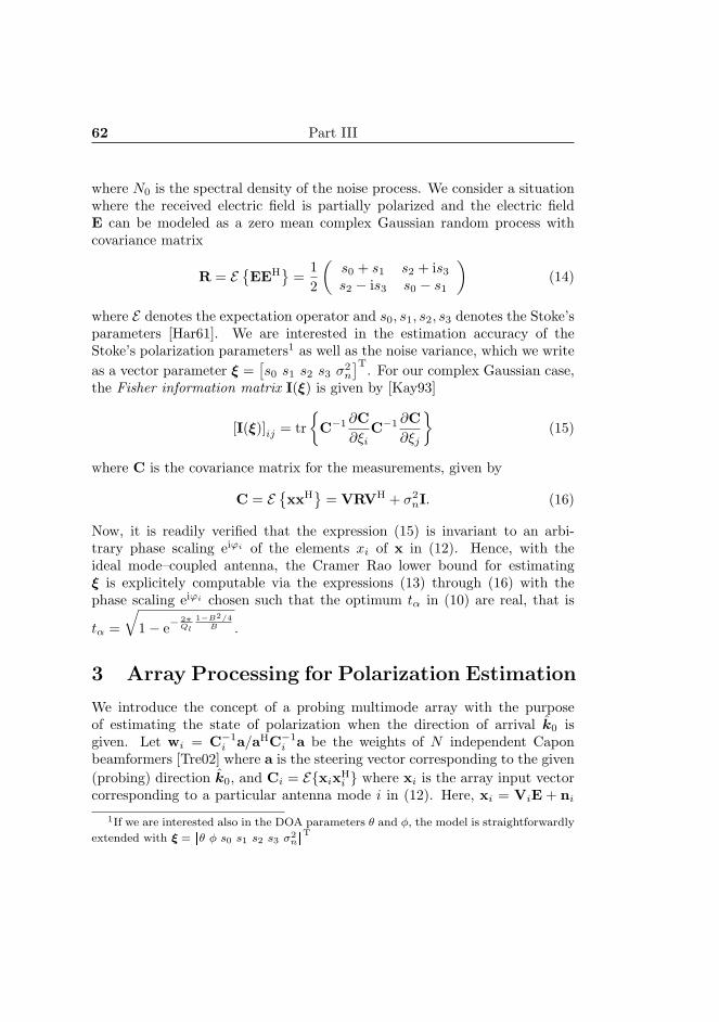
62 Part III

where N0 is the spectral density of the noise process. We consider a situationwhere the received electric field is partially polarized and the electric fieldE can be modeled as a zero mean complex Gaussian random process withcovariance matrix

R = EEEH

=

12

(s0 + s1 s2 + is3

s2 − is3 s0 − s1

)(14)

where E denotes the expectation operator and s0, s1, s2, s3 denotes the Stoke’sparameters [Har61]. We are interested in the estimation accuracy of theStoke’s polarization parameters1 as well as the noise variance, which we writeas a vector parameter ξ =

[s0 s1 s2 s3 σ2

n

]T. For our complex Gaussian case,the Fisher information matrix I(ξ) is given by [Kay93]

[I(ξ)]ij = trC−1 ∂C

∂ξiC−1 ∂C

∂ξj

(15)

where C is the covariance matrix for the measurements, given by

C = ExxH

= VRVH + σ2

nI. (16)

Now, it is readily verified that the expression (15) is invariant to an arbi-trary phase scaling eiϕi of the elements xi of x in (12). Hence, with theideal mode–coupled antenna, the Cramer Rao lower bound for estimatingξ is explicitely computable via the expressions (13) through (16) with thephase scaling eiϕi chosen such that the optimum tα in (10) are real, that is

tα =

√1− e−

2πQl

1−B2/4B .

3 Array Processing for Polarization Estimation

We introduce the concept of a probing multimode array with the purposeof estimating the state of polarization when the direction of arrival k0 isgiven. Let wi = C−1

i a/aHC−1i a be the weights of N independent Capon

beamformers [Tre02] where a is the steering vector corresponding to the given(probing) direction k0, and Ci = ExixH

i where xi is the array input vectorcorresponding to a particular antenna mode i in (12). Here, xi = ViE + ni

1If we are interested also in the DOA parameters θ and φ, the model is straightforwardly

extended with ξ =θ φ s0 s1 s2 s3 σ2

n

T


where Vi =√

Zg

η2πk a ⊗ tiA where ti and ni are the ith rows of T and n,

respectively.It is readily seen that the signal model for the processed signals y =

wHi xi

becomes

y = V0E + ny (17)

where V0 =√

Zg

η2πk TA and ny =

wH

i ni

, and where the covariance matrix

is given byCy = V0RVH

0 + σ2nG (18)

where G is a diagonal matrix with diagonal entries wHi wi. Hence, it is as-

sumed that the processor is able to reject a limited number (less then J)of interferers coming from discrete directions kj , and the remaining noise issensor noise colored by the processor weights.

The Maximum Likelihood (ML) estimator for the situation above can bederived by extending the results in e.g. [Tre02, Jaf88] which are given for thecase when the noise is white and G = I. It is assumed here that the matrixV = V0 has dimension n × m with n > m. Further, let Ry be the samplecovariance matrix based on I independent measurements yi

Ry =1I

I∑i=1

yiyHi . (19)

By extending the derivation in [Tre02] to include a general positively definitecoloration matrix G as above, the ML estimator for (R, σ2

n) can be found as

σ2n =

1n−m

trG−1P⊥V Ry (20)

R = V+(Ry − σ2

nG)

(V+)H (21)

where

P⊥V = I−V

(VHG−1V

)−1VHG−1 (22)

V+ =(VHG−1V

)−1VHG−1 (23)

are the orthogonal projector onto RV⊥ and the pseudoinverse of V,respectively, where the weighted norm based on G−1 is used.

64 Part III

4 Numerical examples

In Fig. 2 is shown the optimum transmission coefficients |tl|2 from (10) withQ–values corresponding to the first 3 mode orders l = 1, 2, 3, cf. [CR64], asthe electrical size ka as well as the fractional bandwidth B is varied. Thefigure illustrates the difficulty to match higher order modes, as well as thefact that all modes will ultimately become useful (useless) as the electricalsize increases (decreases), or as the bandwidth decreases (increases).

In Fig. 3 is shown the Fisher information functional log det I(ξ) based on(15), for a single, ideal tripole antenna with a = 1 and

A =

√38π

cos θ cos φ − sinφcos θ sinφ cos φ− sin θ 0

(24)

corresponding to the three fundamental TM modes of lowest order l = 1,or equivalently, the three ideal electrical dipoles in the cartesian base vectordirections x, y, z. The functional log det I(ξ) is shown as a function of theelectrical size ka with the optimum transmission coefficients tα calculated asin (10) with B = 5 % and Q = 1

ka + 1(ka)3 , cf. [CR64]. The Stoke’s parameters

are parameterized as

s1 = Ps0 cos(2α) cos(2β)s2 = Ps0 cos(2α) sin(2β)s3 = Ps0 sin(2α)

(25)

where 0 ≤ P ≤ 1 is the degree of polarization. The signal–to–noise ratiodefined as SNR = s0

σ2n

Zg

η ( 2πk )2 was chosen to 50 dB. Our study shows that the

estimation performance of the tripole antenna as measured by the functionallog det I(ξ) is invariant to the directional parameters θ and φ as well as tothe polarization parameters α and β. However, the functional log det I(ξ)depends strongly on the polarization degree P , as well as on the electrical sizeka of the antenna and the bandwidth B of the system.


0 0.2 0.4 0.6 0.8 110

-4

10-3

10-2

10-1

100

Optimum transmission coefficient |tl|2

Electrical size ka

l = 1

l = 2

l = 3

Figure 2: Optimum transmission coefficient |tl|2 as a function of electrical sizeka for the first 3 mode orders l = 1, 2, 3. Fractional bandwidth is B = 1, 5, 10%.

66 Part III

10-3

10-2

10-1

100

-10

0

10

20

30

40

50

60

70

80Fisher Information log det(I)

P = 1

P = 0.999

P = 0.99

P = 0.9

P = 0

Electrical size ka

Figure 3: Fisher Information log det(I) as a function of electrical size ka forpolarization degrees P = 1, 0.999, 0.99, 0.9, 0. Fractional bandwidth is B = 5%.

5 Summary

Fundamental physical limitations associated with DOA and/or polarizationestimation using antennas or antenna arrays are analyzed. As a general frame-work for the analysis, spherical vector modes and their associated equivalentcircuits and Q factor approximations are employed together with the broad-band Fano theory. The concept of a probing multimode array is introducedwhich is equivalent to one single multimode antenna without interferers butwith colored noise, and the explicit form of the corresponding ML estimatorfor the state of polarization is given. The log–determinant of the Fisher infor-mation matrix is employed as a measure to evaluate the performance of theideal multimode antenna processor with respect to its ability to estimate thestate of polarization of a partially polarized plane wave coming from a given


direction. Our study shows that the estimation performance of the ideal mul-timode antenna is invariant to the directional parameters as well as to thepolarization parameters for a given polarization degree. However, the estima-tion performance depends strongly on the polarization degree, as well as onthe electrical size of the antenna and the bandwidth of the system.

A Spherical Vector Waves

The outgoing spherical vector waves are given by

u1ml(kr) = hl(kr)A1ml(r)

u2ml(kr) =1k∇× u1ml(kr) =

(krhl(kr))′

krA2ml(r) +

√l(l + 1)

hl(kr)kr

A3ml(r)

(26)where Aτml(r) are the spherical vector harmonics and hl(x) the sphericalHankel functions of the second kind, see [AW01, Jac75, New02]. The sphericalvector harmonics Aτml(r) are given by

A1ml(r) =1√

l(l + 1)∇× (rYml(r))

A2ml(r) = r ×A1ml(r)A3ml(r) = rYml(r)

(27)

where Yml(r) are the scalar spherical harmonics given by

Yml(θ, φ) = (−1)m

√2l + 1

4π

√(l −m)!(l + m)!

Pml (cos θ)eimφ (28)

and where Pml (x) are the associated Legendre functions [AW01]. For negative

m–indices, the scalar waves satisfies the symmetry Y−m,l(r) = (−1)mY∗ml(r),

and henceAτ,−m,l(r) = (−1)mA∗

τml(r). (29)

References

[AW01] George B. Arfken and Hans J. Weber. Mathematical Methods forPhysicists. Academic Press, New York, fifth edition, 2001.

[Chu48] L. J. Chu. Physical limitations of Omni-Directional antennas.Appl. Phys., 19:1163–1175, December 1948.

68 Part III

[CR64] R. E. Collin and S. Rothschild. Evaluation of antenna Q. IEEETrans. Antennas Propagat., 12:23–27, January 1964.

[DPG+98] S. Drabowitch, A. Papiernik, H. Griffiths, J. Encinas, and B. L.Smith. Modern Antennas. Chapman & Hall, 1998.

[Fan50] R. M. Fano. Theoretical limitations on the broadband match-ing of arbitrary impedances. Journal of the Franklin Institute,249(1,2):57–83 and 139–154, jan,feb 1950.

[Fan69] R. L. Fante. Quality factor of general antennas. IEEE Trans.Antennas Propagat., 17(2):151–155, March 1969.

[GJQ00] W. Geyi, P. Jarmuszewski, and Y. Qi. The Foster reactance the-orem for antennas and radiation Q. IEEE Trans. Antennas Prop-agat., 48(3):401–408, March 2000.

[GN04] M. Gustafsson and Sven Nordebo. On the spectral efficiency ofa sphere. Technical Report LUTEDX/(TEAT-7127)/1–24/(2004),Lund Institute of Technology, Department of Electroscience, P.O.Box 118, S-211 00 Lund, Sweden, 2004. Submitted to IEEE Trans.on Antennas and Propagation.

[Han81] R. C. Hansen. Fundamental limitations in antennas. Proc. IEEE,69(2):170–182, 1981.

[Har61] R. F. Harrington. Time Harmonic Electromagnetic Fields.McGraw-Hill, New York, 1961.

[HN95] B. Hochwald and A. Nehorai. Polarimetric modeling and param-eter estimation with applications to remote sensing. IEEE Trans.Signal Processing, 43(8):1923–1935, August 1995.

[HTN99] K-C Ho, K-C Tan, and A. Nehorai. Estimating directions of arrivalof completely and incompletely polarized signals with electromag-netic vector sensors. IEEE Trans. Signal Processing, 47(10):2845–2852, October 1999.

[HTT97] K-C Ho, K-C Tan, and B. T. G. Tan. Efficient method for es-timating directions–of–arrival of partially polarized signals withelectromagnetic vector sensors. IEEE Trans. Signal Processing,45(10):2485–2498, October 1997.


[HTT98] K-C Ho, K-C Tan, and B. T. G. Tan. Linear dependence of steer-ing vectors associated with tripole arrays. IEEE Trans. AntennasPropagat., 46(11):1705–1711, November 1998.

[Jac75] J. D. Jackson. Classical Electrodynamics. John Wiley & Sons,New York, second edition, 1975.

[Jaf88] A. G. Jaffer. Maximum likelihood direction finding of stochasticsources: A separable solution. In 1988 IEEE International Con-ference on Acoustics, Speech, and Signal Processing, pages 2893–2896. IEEE Signal Processing Society, 1988.

[Kar03] Anders Karlsson. Physical limitations of antennas in a lossymedium. Technical Report LUTEDX/(TEAT-7114)/1–15/(2003),Lund Institute of Technology, Department of Electroscience, P.O.Box 118, S-211 00 Lund, Sweden, 2003.

[Kay93] S. M. Kay. Fundamentals of Statistical Signal Processing, Estima-tion Theory. Prentice-Hall, Inc., NJ, 1993.

[KV96] H. Krim and M. Viberg. Two decades of array signal process-ing research: the parametric approach. IEEE Signal ProcessingMagazine, 13(4):67–94, July 1996.


[LS94] J. Li and P. Stoica. Efficient parameter estimation of partiallypolarized electromagnetic waves. IEEE Trans. Signal Processing,42(11):3114–3125, November 1994.

[McL96] James S. McLean. A re-examination of the fundamental limitson the radiation Q of electrically small antennas. IEEE Trans.Antennas Propagat., 44(5):672–676, May 1996.

[Mil74] K. S. Miller. Complex Stochastic Processes. Addison–Wesley Pub-lishing Company, Inc., 1974.

[New02] Roger G. Newton. Scattering Theory of Waves and Particles.Dover Publications, New York, second edition, 2002.

70 Part III

[NG04] Sven Nordebo and M. Gustafsson. Fundamental limitations forDOA estimation by a sphere. Technical Report LUTEDX/(TEAT-7128)/1–26/(2004), Lund Institute of Technology, Department ofElectroscience, P.O. Box 118, S-211 00 Lund, Sweden, 2004. Sub-mitted to IEEE Trans. on Signal Processing.

[NG05] Sven Nordebo and Mats Gustafsson. Multichannel broadbandFano theory for arbitrary lossless antennas with applications inDOA estimation. In 2005 IEEE International Conference onAcoustics, Speech, and Signal Processing. IEEE Signal ProcessingSociety, 2005. (Accepted for publication).

[SN90] P. Stoica and A. Nehorai. Music, maximum likelihood, and cramer-rao bound: further results and comparisons. IEEE Trans. Acous-tics, Speech, and Signal Processing, 38(12):2140–2150, December1990.

[SV93] A. Swindlehurst and M. Viberg. Subspace fitting with diverselypolarized antenna arrays. IEEE Trans. Antennas Propagat.,41(12):1687–1694, December 1993.

[Tha78] H. L. Thal. Exact circuit analysis of spherical waves. IEEE Trans.Antennas Propagat., 26(2):282–287, March 1978.


[VSO97] M. Viberg, P. Stoica, and B. Ottersten. Maximum likelihood ar-ray processing in spatially correlated noise fields using parameter-ized signals. IEEE Trans. Signal Processing, 45(4):996–1004, April1997.

[WF93] A. J. Weiss and B. Friedlander. Maximum likelihood signal esti-mation for polarization sensitive arrays. IEEE Trans. AntennasPropagat., 41(7):918–925, July 1993.

[WLZ04] K. T. Wong, L. Li, and M. D. Zoltowski. Root–MUSIC–baseddirection–finding and polarization estimation using diversely po-larized possibly collocated antennas. IEEE Antennas & WirelessPropagation Letters, 3(8):129–132, 2004.


[Won01] K. T. Wong. Direction finding/polarization estimation – dipoleand/or loop triad(s). IEEE Transactions on Aerospace and Elec-tronic Systems, 37(2):679–684, April 2001.

[WZ00] K. T. Wong and M. D. Zoltowski. Closed–form direction findingand polarization estimation with arbitrarily spaced electromag-netic vector–sensors at unknown locations. IEEE Trans. AntennasPropagat., 48(5):671–681, May 2000.

Part IV

On Fault Localization onPower Lines - An FMCW

Based Fault Locator

Part IV is published as:

J. Lundback, S. Nordebo, M. Akke, T. Biro, ”On Fault Localization on PowerLines - An FMCW Based Fault Locator”, Research Report 05030, ISSN 1650-2647, VXU/MSI/EL/R/–05030/–SE, Vaxjo university, April 2005.

On Fault Localization on Power Lines -

An FMCW Based Fault Locator

J. Lundback, S. Nordebo, M. Akke, T. Biro

Abstract

In this report we consider using frequency modulated continuouswaves to locate a one line to ground fault on a power line. We modelthe power line using transmission line theory combined with Carson’smodel for the frequency dependent transmission line parameters in twobasic configurations. Simulations using different frequency estimationalgorithms are presented and compared with the Cramer-Rao Bound.Measurements using a fault locator in a laboratory environment and ina field-experiment are also studied. It is observed that fault-locationestimation with high accuracy is possible using limited bandwidth.

1 Introduction

In this report we present a Frequency Modulated Continuous Wave (FMCW)fault locator for power lines using transmission line theory as well as mea-surements to exemplify the concept. In microwave technology, FMCW radarrepresents one of the oldest, simplest but also one of the most versatile typesof radar, cf. [Gri90, Sto92]. Even though the basic ideas and advantages ofusing FMCW radar techniques for power line fault localization were estab-lished already in [DST72] and revived for optical fibre systems in [UC85], theapplication area for transmission lines still seems to be vastly unexplored.

In our view, the FMCW radar techniques for power line fault localizationhas a great potential mainly because of the versatile time-bandwidth prop-erty that can be exploited to achieve high accuracy in situations where theusable bandwidth is limited but the measurement time is less critical. Thus,by averaging over many successive frequency sweeps a high signal–to–noise–ratio SNR is readily obtained which is required for obtaining good estimationperformance. Further, the FMCW approach converts the distance-to-fault

74

On Fault Localization on Power Lines - An FMCW Based Fault Locator 75

estimation into a frequency estimation issue in which several high-resolutionalgorithms e.g. ESPRIT, CAPON, MUSIC, Prony, etc., [PS97, PG01, AW02,MB94, Kay87, Tre02] that can be utilized to obtain high accuracy.

Today, there exist functional systems for fault localization, but there isalso a pronounced demand from the power industry to significantly improvethe cost, efficiency and accuracy of these systems. This is probably the rea-son to the relatively large amount of research pursued on this topic over thelast 10 years. However, most of the research results are concerned with 50Hz impedance measurements or transient analysis up to a few kHz, see e.g.[AGH00, BG04] and references therein, and does not take into account thepossibility of exploiting travelling waves which are relevant for much widerfrequency ranges.

Our work is based on a previous study in [AB04] where measurementsof the frequency dependent impedance of a thin wire of length 1.5 km withground return were performed. The measurement setup is considered as adownscaled experimental setup of the phenomena’s occurring on real powerlines since the models used are valid for a general set of geometries. In [AB04],the experimental results are compared with mathematical models for powerlines such as given in e.g. [Car26]. For frequency intervals relevant for powerline transients, a discrepancy is observed between the experimental resultsand the models. It is noted that the model in [Car26] is based on the as-sumption that the length of the wire is much longer than the wave lengthsconsidered. Hence, this condition cannot always be assumed to hold in thecase of grounding faults in power distribution systems. Furthermore, it isconcluded that the dynamics of the grounding system should be incorporatedin the model.

In the present study, we have performed an additional field test and mea-surement campaign on the thin wire with ground return in order to verifythe possibility of exploiting the FMCW range estimation techniques to mea-sure the distance to ground fault. Since neither the measurement nor theestimation strategies has been optimised we expect that these results can beimproved significantly in future studies.

Next, we give a survey of some existing fault localization methods. Insection 2 we start by developing a signal model using transmission line theoryand Carson’s model for the fundamental case of a wire or line with unknownlength connected to a load impedance. Thereafter, in section 3 we examine theoptimal performance that can be expected from any unbiased estimator usingthe Cramer-Rao Bound (CRB) and corresponding simulations that exploit thefrequency estimation algorithms of section 4. The signal model is then verified

76 Part IV

experimentally using coaxial cables, section 6.1. In section 6.2 we account fora field-experiment using a downscaled power line setup and present somerelated results. Finally, in section 7 we expand the signal model from section2 to a more realistic but still limited situation and present calculations of theoptimal performance together with simulations.

1.1 Survey on fault localization

A transmission system is a high voltage system (50–400 kV), usually directlyearthed, with power lines of a length typically ranging from 100 km to 600km. The distribution systems are medium voltage systems (10–50 kV), usuallyhigh–resistance earthed, with power lines of a length typically ranging from100 m to 20 km. Hence, the requirements for fault localization in transmissionsystems are fundamentally different than for distribution systems.

ASEA (now ABB) pioneered the development of impedance based faultlocators for transmission systems in the beginning of the 1980’s, see [LER85].Initially, the fault locator was installed as a separate box but has later been in-tegrated in the distance protection terminals. The installed base of separateand integrated fault locators amounts to more than 10000 units worldwidetoday. Manufacturers claim that the impedance based fault locators can de-termine the distance to fault with an accuracy of 1 to 3 %. However, users offault locators now want to determine the tower where the fault has occurredso that the maintenance crew knows exactly where to go and can take thefastest route to the fault location. This means that there is a need to improvethe accuracy of fault locators. The distance between towers on transmissionlines is in the order of 300 m and the transmission line may have a length upto 600 km. This means that the desired accuracy is in the order of 0.05 %or at least one order of magnitude better than the existing impedance basedfault locators. The introduction of series capacitors on transmission lines isone method to increase the transfer capability of a transmission system with-out using additional line corridors. On a series compensated line, there is nolonger a unique relation between the physical distance to the fault locationand the measured electrical reactance measured by an impedance based faultlocator. This means that an impedance based fault locator gives more thanone possible fault location and additional information must be collected andprocessed before the maintenance crew can be directed to the fault location.The advent of the GPS and GLONASS, see [Wil91, Wil92, YGGB91] makes itpossible to determine the arrival of fault generated transients with an absoluteaccuracy of 1 microsecond or better. This has paved the way for travelling


wave based fault locators. The accuracy of future travelling wave based faultlocators may be an order of magnitude better than the accuracy of impedancebased fault locators. Future travelling wave-based fault locators may also beapplied on series compensated lines and they will provide a unique fault loca-tion. Different kinds of fault generated transients are discussed in [Leh92]. Asingle phase–to–earth fault generates a significant ground mode while a phase–to–phase short circuit generates a significant aerial mode. Aerial modes travelwith a speed that is close to the speed of light while ground modes travel witha lower speed. The design of a travelling wave based fault locator requires agood understanding of wave propagation on power lines. The main issues are:(1) the wave propagation speed of aerial and ground modes, (2) the damp-ing of aerial and ground modes, and (3) the distortion of the fault generatedwaveform, and (4) the scattering of waves at discontinuities along power lines.

Methods for fault localization such as the impedance based measurementtechniques in [LER85] are applicable for transmission systems where the earth–fault currents are high as well as stationary. However, these methods are notdirectly applicable to distribution systems that are often earthed using high–ohm inductors. This is one of the main reasons that the development of faultlocalization techniques for distribution systems is an area of great industrialas well as academic potential today. To this end, the measurement of faultinduced transients is a very interesting possibility [Leh92]. However, the dis-tribution lines are relatively short (100 m to 20 km) and the number of lines isseveral orders of magnitude greater than for transmission systems. The pro-tect terminals for distribution systems are also much more primitive than fortransmission systems. The fault location equipment must therefore be verycheap and simple to mount.

It is also noted that the future trend in the power industry is to replacethe overhead power lines by buried cables. In contrast to failures on overheadpower lines, cable faults are often permanent. Thus, the faulty cable has to beexcavated and a fault localization system of very high accuracy will thereforebe required. Conventional techniques today use pulse radar to estimate faultlocation. However, since buried cables usually have very low bandwidth com-pared to overhead power lines, this is further a motivation to study FMCWradar as a high resolution ranging technique.

Even though the theory for travelling waves on power lines is a rela-tively well established area, see e.g. [Lun95, RGOC00] it appears that re-mote sensing of transients as well as precision reflectometric methods such as[DST72, UC85] is a vastly unexplored area for fault localization. In [Lun95],direct and inverse problems for non-uniform transmission lines with internal

78 Part IV

transient voltage and current sources are considered. In the inverse sourceproblem, the compact Green functions approach based on wave splitting isused to reconstruct the transient voltage and current sources from the tran-sient signals that are received at the two endpoints of the transmission line.However, in [Lun95] the location of the sources is assumed to be known.Hence, here is an apparent potential to consider inverse scattering problemsfor the location of transient sources on transmission lines.

2 Signal Model

In this section we develop a signal model describing the signals that we utilizeto estimate the distance d to a fault or impedance discontinuity. Thereafter, insection 2.1 we model the parameters of the transmission line using Carson’smodel [Car26]. The schematics of the signal model is depicted in figure 1

Figure 1: Schematics of the signal model. The FMCW signal, the bufferand the generator impedance are user parameters. The transmission lineparameters are described by Carson’s model.

and is considered to be a simplified model of a section of a faulted powerline. We consider the load impedance ZL in this setup to be equivalent toa fault impedance in the case of a faulted power line system. Thereby werestrict our investigations to include one line to ground faults (1LG) [And98].This configuration constitutes a first approach that we can easily verify bothexperimentally and by simulations.

The linear FMCW radar signal is

s(t) = Ace−jφ(t), (1)


where Ac is the real amplitude and

φ(t) = 2π

∫ t

0

(f0 + aτ) dτ = 2π(f0t +

a

2t2

)(2)

is the instantaneous phase. The Frequency Modulation (FM) rate a = B/Twhere B is the bandwidth of operation, T is the period time of s(t) duringwhich one frequency sweep is completed and f0 is the frequency at time t = 0or the start frequency of any successive period of s(t). We apply s(t) to atransmission line, see figure 1, and exploit that we can model the transmissionline as a linear system with a frequency response that is dependent on themeasurement position on the transmission line. In point B, figure 1, thefrequency response of the transmission line is, [Poz98]

H(ω) =Z0

Z0 + ZG

1 + ΓLe−2γd

1 − ΓGΓLe−2γd, (3)

where ω is the angular frequency, Z0 the characteristic impedance of thetransmission line, ZG the output impedance of the FMCW signal generator,ZL the load impedance considered to be caused by a fault,

ΓG =ZG − Z0

ZG + Z0(4)

and

ΓL =ZL − Z0

ZL + Z0, (5)

the reflection coefficients at the generator impedance and the load impedance,respectively. Further, γ is the complex propagation constant and d is thedistance from ZG to ZL. The parameters Z0 and γ in (3) are dependent onω. The signal measured at point B in figure 1 is

y(t) =

∫ t

0

h(τ)s(t − τ)dτ = Ace−j2π(f0t+ a

2 t2)

∫ t

0

h(τ)ej2π(f0τ+aτt)e−j2π a2 τ2

dτ,

(6)where h(t) is the impulse response corresponding to H(ω). We choose a so thataτ2

h << 1 where τh is the total duration time of h(τ). Then, for τh ≤ t ≤ T

y(t) ≈ Ace−j2π(f0t+ a

2 t2)

∫ τh

0

h(τ)ej2π(f0+at)τdτ = Ace−j2π(f0t+ a

2 t2)H∗(2π(f0+at)),

(7)

80 Part IV

where ∗ denotes the conjugate. The Intermediate Frequency (IF) signal[Sto92] is given by

x(t) = s∗(t)y(t) = A2cH

∗(2π(f0 + at)). (8)

Observe that x(t) corresponds to the frequency response of the transmissionline with the characteristics of ZL included.

We obtain the discrete-time signal

x(n) = A2cH

∗(ωn), (9)

by sampling x(t) in t = nTs, n = 0, 1, 2..., N − 1, Ts = 1/fs where fs is thesampling frequency, N the number of samples and ωn = 2π(f0+anTs) = ω0+2πanTs. Further, H∗(ωn) can be expressed as a sum of complex exponentialsusing the formula for a geometric sum,

H∗(ωn) =Z0

Z0 + ZG

+∞∑

m=1

(Z0

Z0 + ZG

ΓmL Γm−1

G (1 + ΓG))∗e−2γ∗dm. (10)

Next, from [Poz98],

γ =√

(r + jωl)(jωc) ≈r

2

√c

l+ jω

√cl (11)

where r, l, c are the frequency dependent transmission line parameters, specif-ically r [Ω/m] is the resistance, l [H/m] the inductance and c [F/m] the ca-pacitance, respectively. We have assumed that the conductance is zero ornegligible. Using (10) and (11) we rewrite (9) as

x(n) = A2c

Z0

Z0 + ZG

+∑

m

Ame(−r√

cl+j2ωn

√cl)dm (12)

where

Am = A2c

(Z0

Z0 + ZG

ΓmL Γm−1

G (1 + ΓG)

)∗

. (13)

To handle an infinite number of exponentials in (10) is impractical and de-pending on the attenuation per meter and the length of the transmission line,the number of exponentials that must be considered to obtain a reasonablemodel will vary. In (12) we therefore assume that we need a finite number ofexponentials to model the transmission line with a good accuracy. Observethat x(n) is a harmonic progression of damped complex exponentials wherethe damping and frequency depends on r, l, c, a and d.


2.1 Carson’s Model of the Transmission Line Parameters

We calculate the transmission line parameters according to Carson’s electro-magnetic model of a thin wire above ground with ground return as [Car26],

r = r0 + rf , (14)

l = l0 + lf , (15)

c = c0. (16)

Here, r0, l0 and c0 represent the transmission line parameters when the earthis a perfect conductor while rf and lf are contributions due to the earthsfinite conductivity. Further, using [Car26, And95] we calculate

r0 =ρ

A[Ω/m] , (17)

l0 = 2 · 10−7 ln

(h

0.779z

)[H/m] , (18)

c0 =55.8 · 10−12

ln(2h/z)[F/m] , (19)

where ρ, z, A are the resistivity, the radius and the cross-section area of thetransmission line, respectively, and h is the height of the transmission lineabove the ground. Observe that in Carson’s model rf and lf are frequencydependent while c is not and we obtain rf and lf from e.g. [Car26, And95] bycalculations. In figures 2 and 3 the values of r and l are displayed as functionsof frequency using an FK 1.5 mm2 copper cable. The earth resistivity is1000 Ω/m and h = 1 m. These values are used in the measurements describedin section 6.2.

From calculations of r and l, similar to the one displayed in figure 2 and3, and from the corresponding equations in [Car26] we observe that r is ap-proximately a linear function of frequency and l, although not frequency in-dependent, does not display a large variation over the frequency interval ofoperation. We therefore set

r = r1ω + r2, (20)

l = mean l(ω) , (21)

i.e. we approximate r as a linear function of frequency and l as a constant,equal to the mean value within the frequency interval of operation, see the

82 Part IV

100 120 140 160 180 200 220 240 260 280 3000.1

0.15

0.2

0.25

0.3

0.35

Frequency [kHz]

r [Ω

/m]

Figure 2: Resistance r [Ω/m] according to Carson’s model.

dashed curve in figure 3. Using (20) and (21) we can rewrite (12) as

x(n) = A2c

Z0

Z0 + ZG

+

M∑

m=1

AmePme(−βn+jΩn)m, n = 0, ..., N − 1, (22)

where

P = −d(r1ω0 + r2)

√c

l+ j2ω0d

√cl, (23)

β = 2πar1dTs

√c

l, (24)

Ω = 4πadTs

√cl. (25)

Finally, as a consequence of the approximations made regarding r and l thecharacteristic impedance Z0, depicted in figures 4 and 5, is affected as seenby comparing the solid line with and the dashed curve in both figures, respec-tively. Based on the figures we set Z0 = Z0(2πfa) where fa = 200 kHz or the


100 120 140 160 180 200 220 240 260 280 3002.1

2.12

2.14

2.16

2.18

2.2

2.22

2.24

Frequency [kHz]

l [µH

/m]

Figure 3: Inductance l [H/m] according to Carson’s model. The solid linecorresponds to l given by Carson’s model and the dashed line is an approxi-mation.

median frequency of the frequency interval of operation.We see in (22) that x(n) consists of damped complex exponentials or

damped cisoids with constant amplitudes Am (provided that ZG and ZL arefrequency independent) where d is part of e.g. the fundamental frequency Ω(25). The assumptions regarding the transmission line parameters obtainedusing Carson’s model results in travelling waves with constant phase velocity.This assumption is often made in Time Domain Reflectometry (TDR) wherea pulse is used to estimate the time taken to propagate back and forth on thetransmission line. In practice, the assumption of constant phase velocity inTDR is less likely to hold since the pulse is a wideband signal even thoughthe pulse can be made more narrowband by pulse shaping. Further, TDR re-quires a decision algorithm to estimate when the pulse returns because of thepulse shape distortion. The use of the FMCW radar technique can mitigatethe difficulties in TDR since the bandwidth of the chirp can be chosen smallcompared with the bandwidth of the pulse in TDR.

84 Part IV

100 120 140 160 180 200 220 240 260 280 300548

550

552

554

556

558

560

562

564

Frequency [kHz]

abs

Z 0 [Ω]

Figure 4: The modulus of Z0. The solid curve corresponds to frequency de-pendent r and l according to Carson’s model without approximations, thedashed curve corresponds to r and l according to the approximations above,and the dash-dotted line corresponds to |Z0(2πfa)|.

100 120 140 160 180 200 220 240 260 280 300−2.3

−2.25

−2.2

−2.15

−2.1

−2.05

Frequency [kHz]

arg

Z 0 [deg

]

Figure 5: The phase of Z0. The solid curve corresponds to frequency depen-dent r and l according to Carson’s model without approximations, the dashedcurve corresponds to r and constant l according to the approximations above,and the dash-dotted line corresponds to the phase of Z0(2πfa).


3 Cramer-Rao Bound

In this section we derive the CRB of d using Carson’s model. We assume thatthe signal is distorted by complex White Gaussian Noise (WGN) v(n), withzero mean and variance σ2

v , so that

x(n) = A2cH

∗(ωn) + v(n). (26)

We can represent the samples on vector form as x = [x(0) . . . x(N − 1)]T

whereT denotes the transpose operation. The mean-value vector µ and covariancematrix C of x are

[µ]k = E [x]k = A2cH

∗(ω(k−1)), k = 1 . . . N, (27)

C = E

(x − µ)H

(x − µ)

= σ2vIu, (28)

where Iu is the unity matrix, E · and (·)H denotes the expectation operatorand Hermitian transpose, respectively. The CRB of d is given by CRB d =I−1 where I is the Fisher information and is calculated as [Kay93],

I =2

σ2v

∥∥∥∥∂µ

∂d

∥∥∥∥2

, (29)

where ‖·‖ denotes the Euclidean norm. We define the signal-to-noise ratio(SNR) as

SNR =

(A2

c

σv

)2

. (30)

Observe that the FMCW signal reflected at ZL is attenuated depending on dso the effective SNR is depending on the distance to the fault location. Byeffective SNR we mean the ratio of the power of the fundamental harmonicin (22) to the noise power σ2

v . The effective SNR is therefore always lowerthan the SNR we use and display. In reality we can control the power ofthe FMCW signal or equivalently the SNR, as we defined it, and from thecharacteristics of the transmission line we might be able to select the SNRso that the effective SNR is sufficiently large for the estimation algorithms towork properly.

Further, in the calculations, if nothing else is stated, ZG = 470 Ω, ZL =51 Ω, B = 200 kHz, Ac = 1 V, T = 1 ms, N = 126 and SNR=50 dB. Figure

86 Part IV

30 40 50 60 70 80 900

0.05

0.1

0.15

0.2

0.25

0.3

0.35

0.4

0.45

0.5

Opt

imal

RM

SE

[% o

f dis

tanc

e]

SNR [dB]

Figure 6: Optimal RMSE as a function of SNR. An increase in the SNR de-creases the optimal RMSE. The solid curve corresponds to d = 1000 m, thedashed curve corresponds to d = 5000 m and the dash-dotted curve corre-sponds to d = 10000 m.

6 depict the optimal Root Mean Square Error (RMSE) as a function of theSNR where the optimal RMSE is measured in percentage of d i.e.

Optimal RMSE d =

√CRB d

d· 100 [%] . (31)

Observe that the CRB is calculated using one measurement of one period ofthe FMCW signal. In figure 6 the effect of increasing the SNR on the optimalRMSE is displayed. It is concluded that the increase in SNR decreases theoptimal RMSE and that a SNR larger than 50 dB result in a optimal RMSElower than 0.1 %.


0 1000 2000 3000 4000 5000 6000 7000 8000 9000 100000.01

0.02

0.03

0.04

0.05

0.06

0.07

0.08

0.09

0.1O

ptim

al R

MS

E [%

of d

ista

nce]

Distance d [m]

Figure 7: Optimal RMSE as a function of d. The solid line corresponds toB = 200 kHz, the dashed line corresponds to 500 kHz and the dash-dottedline corresponds to 800 kHz.

Figure 7 depicts the optimal RMSE as a function of d, the solid curvecorresponds to B = 200 kHz, the dashed curve to 500 kHz and the dash-dottedcurve to 800 kHz. Observe the low values of the optimal RMSE which indicatethat a high-resolution estimate of d can be achieved. The calculations indicatethat a higher bandwidth result in a lower RMSE for short distances but anincrease of the RMSE for longer distances. Observe that the attenuation ofthe harmonics in x(n) is proportional to d · B. Therefore will the optimalRMSE increase for larger d and B.

88 Part IV

100 150 200 250 300 350 400 450 500 5500.01

0.02

0.03

0.04

0.05

0.06

0.07

0.08

0.09

0.1

Opt

imal

RM

SE

[% o

f dis

tanc

e]

Number of samples

d=10000 m

d=1000 m

Figure 8: Optimal RMSE as a function of N. The solid line corresponds toB = 200 kHz, the dashed line corresponds to 500 kHz and the dash-dottedline corresponds to 800 kHz.

One possibility that increases the flexibility is to keep B constant andchange T that must be adjusted according to the maximum length of thetransmission line and the sample rate. Increasing the number of samples perperiod of the FMCW signal will increase the performance as seen in figure 8.The solid curve corresponds to B = 200 kHz, the dashed curve to 500 kHzand the dash-dotted curve to 800 kHz. The three upper curves corresponds tod = 10000 m and the three lower curves corresponds to d = 1000 m. Observethat the curves corresponding to B = 500 kHz and B = 800 kHz for d = 1000are approximately equal. The effect of increasing N is visible in all six curvesbut a larger enhancement of the performance is obtained when d = 10000 mcompared to d = 1000 m. This is most likely related to the lower effectiveSNR obtained when d = 10000 compared d = 1000.


4 Frequency Estimation Algorithms

In this report we utilize the following frequency estimation algorithms; FastFourier Transform (FFT), CAPON, MUltiple Signal Classification (MUSIC)and Estimation of Signal Parameters via Rotational Invariance Techniques(ESPRIT). In our application the signal of interest x(n) is a sum of expo-nentially damped cisoids. Therefore, depending on the value of the dampingthe characteristics of x(n) might not be those of an undamped cisoid that thehigh-resolution algorithms were originally designed for. We therefore expectthat the performances of these algorithms are not optimal. But the algo-rithms are still usable in this preliminary study to evaluate the concept andinvestigate if they can be used on short distances where the damping is lowercompared to longer distances. If so, high-resolution algorithms might be usedas a complement to a non-parametric method to produce a more accurate fre-quency estimate based on the estimate of the first method. Observe that herewe are only concerned with finding the frequency of the fundamental cisoidin (22). This corresponds to the frequency with the maximum power, whichcould also be located as the lowest frequency with power above a predefinedthreshold.

The FFT algorithm, see e.g. [PS97, Kay87], is a well known non-parametricalgorithm with a high degree of robustness and low complexity but the perfor-mance can be degraded by spectral leakage. This is not a major disadvantagehere because the cisoids in x(n) are, if several cisoids exist, separated in fre-quency proportional to d. Several methods e.g. windowing can be used tomitigate these effects in such a case.

CAPON, MUSIC and ESPRIT are all based on the autocorrelation matrixR that we estimate as

R =1

L

L−1∑

l=0

x(l)xH(l), (32)

wherex(l) = [x(l) . . . x(l + M − 1)], L = N − M + 1, (33)

and M is a user-parameter in the estimation methods. Observe that weutilize only one period of x(n). By using several versions of x(n) obtainedfrom synchronized measurement we could effectively increase the SNR.

90 Part IV

4.1 CAPON

The CAPON spectral estimator, see e.g. [PS97, YH04], belongs to the familyof Matched Filterbanks (MAFI) that has been shown to exhibit robustnessagainst model errors. The size of the filter or number of coefficients M isa user-parameter and in [LS96] it has been empirically shown that M couldbe chosen as N/4 ≤ M ≤ N/2 to obtain a good performance. Here, wechoose M = N/4. To obtain the CAPON estimator we consider the followingoptimization formulation,

minh

hHRh subjected to h

Ha(ω) = 1, (34)

where a(ω) = [1ejω . . . ejω(M−1)]T . When solved we obtain the optimal weight-vector or the coefficients of the matched filter as

hc =R

−1a(ω)

aH(ω)R−1a(ω). (35)

This is reinserted into in (34) to obtain a power spectral estimate using (32),

Pc(ω) =1

aH(ω)R−1a(ω). (36)

We can now estimate the frequency of the strongest harmonic in x(n) as

ωd = arg maxω

|Pc(ω)| . (37)

4.2 ESPRIT and MUSIC

ESPRIT and MUSIC are high-resolution parametric algorithms that can givevery good accuracy but which are sensitive to model errors, see e.g. [PS97,Tre02] for several references on the topics. It has been verified that ESPRIThas similar statistical accuracy and performance as MUSIC but do not havethe problem of false frequency estimates that MUSIC exhibit. Both methodsrequire knowledge about the number of cisoids present in x(n) and for thisapplication we decide that there is only one dominant cisoid. Both methodsare based on the properties of the eigenvalues and eigenvectors of R. Let

R = UsDsUHs + UvDvU

Hv , (38)


be the eigenvalue decomposition of R, Ds = diag [λ1 . . . λK ]and Dv = diag [λK+1 . . . λM ] where

λm = λm + σ2v , m = 1...K, (39)

λm = σ2v , m = K + 1...M, (40)

(41)

are the eigenvalues of R. Further,

Us = [u1 ... uK ] (42)

contains the eigenvectors corresponding to λk , k = 1...K which spans thesignal subspace. Further,

Uv = [uK+1 ... uM ] (43)

contains the eigenvectors corresponding to λk , k = K +1...M which spans thenoise subspace. The signal subspace and the noise subspace are orthogonalsince the M eigenvectors corresponding to an M × M hermitian matrix aremutually orthogonal. From the eigenvalue decomposition of (32) we obtainthe MUSIC power spectral estimate as

Pm(ω) =1

aH(ω)UvUHv a(ω)

, (44)

and the desired frequency using (37) with Pc(ω) replaced by Pm(ω).The ESPRIT method estimates the frequencies from solving [PS97]

Us2 = Us1Φ, (45)

for Φ, where Us2 equals Us with the first row deleted and Us1 equals Us withthe last row deleted. Further, Φ = C

−1DC where C is a non-singular matrix

and D = diag[ejω1 ...ejωK

]is the matrix describing the rotation of the signal

structure that ESPRIT is based on, see [PS97] for further details. Observethat this rotation is constructed for undamped cisoids. We obtain estimatesof the frequencies as the arguments of the eigenvalues of the matrix Φ, whichare equal to the arguments of the diagonal elements of D. Solving (45) usingthe eigenvalue decomposition of (32) and a Least-Square approach assumingthat Us1 has full column rank gives,

Φ =(U

Hs1Us1

)−1

UHs1Us2. (46)

Since we only search for one cisoid K = 1 and Φ = φ is a scalar and we obtainωd = arg φ , where arg · is the argument operation.

92 Part IV

5 Simulations

Using (25) we can estimate d as

d = ηf , (47)

where

η =1

2a√

cl(48)

is the scaling factor from frequency to distance and f = Ω/(2πTs) is a fre-quency estimate of the strongest harmonic in x(n) corresponding to the fre-quency of the fundamental harmonic in (22). Observe that both c in (16) andl in (21) used in (48) are frequency independent and constant. The resolution

of d is∆d = η∆f (49)

and can be changed by altering a = B/T or ∆f which is the frequencyresolution of the frequency estimation algorithm.

We perform a Monte Carlo simulation using 100 iterations for each valueplotted. Samples of x(n) are obtained using (26) and values of r, l and ctherein are obtained using (14)-(16) without approximations. Further, ZL =51 Ω, ZG = 470 Ω, B = 200 kHz, T = 1 ms, N = 126, ∆f = 10 Hz andSNR= 50 dB if nothing else is stated.


1000 2000 3000 4000 5000 6000 7000 8000 9000 10000

0

0.5

1

1.5

2

2.5

RM

SE

[% o

f dis

tanc

e]

Distance d [m]

Figure 9: The RMSE for FFT (solid curve with dots), CAPON (dashed curve),MUSIC (dash-dotted curve) and ESPRIT (solid curve with + marker). Thesolid curve corresponds to the optimal RMSE. Here, B = 200 kHz.

In figure 9 and figure 10 the RMSE of d is displayed as a function of d forB = 200 kHz and B = 800 kHz, respectively. Note that in figure 9 the RMSEis only slightly decreased when d increases. Therefore the RMSE measuredin meters is increased for longer distances. In figure 10, B = 800 kHz andthe RMSE of FFT, MUSIC and ESPRIT decreases nearly linear with thedistance. This indicates a nearly constant RMSE measured in meters. Also,ESPRIT and MUSIC are seen to be the best estimators in this simulationbut this can be related to the property of returning biased estimates whenthe signal is not a pure undamped cisoid. However, for short distances thefour algorithms have similar performance. In both figures we observe thatthe values of the RMSE indicate an overall good accuracy depending on thechoice of B and FFT is a natural choice of frequency estimation algorithmbased on simulations and robustness. Moreover, the CAPON method can beexpanded to account for the damping property [YH04] but this increases thecomplexity and computational power needed.

94 Part IV

1000 2000 3000 4000 5000 6000 7000 8000 9000 10000

0

0.5

1

1.5

2

2.5

RM

SE

[% o

f dis

tanc

e]

Distance d [m]

Figure 10: The RMSE for FFT, solid curve with dots), CAPON (dashedcurve), MUSIC (dash-dotted curve) and ESPRIT (solid curve with + marker).The solid curve corresponds to the optimal RMSE. Here, B = 800 kHz.


1000 2000 3000 4000 5000 6000 7000 8000 9000 10000

0

0.5

1

1.5

2

2.5

RM

SE

[% o

f dis

tanc

e]

Distance d [m]

Figure 11: The RMSE for FFT (solid curve with dots), CAPON (dashedcurve), MUSIC (dash-dotted curve) and ESPRIT (solid curve with + marker).The optimal RMSE is the solid curve. Here, B = 200 kHz and T = 0.25 ms.

In figure 11 we set T = 0.25 ms and B = 200 kHz to obtain the same FMrate a as in figure 10. Comparing figure 11 and 10 we see that the performanceof the algorithms are decreased, indicating that the increase of B result in abetter accuracy than the decrease of T.

For shorter distances a must be chosen large enough so that we are ableto record sufficient information about x(n) during one period or T s of theFMCW signal. In figure 12, B = 800 kHz corresponding to the same case asin figure 10 but now for shorter distances. As seen, the algorithms are notable to achieve the same accuracy for shorter distances compared to longerdistances where the fundamental harmonic of x(n) has a higher frequency andsufficient information can be recorded during T s.

96 Part IV

200 400 600 800 1000 1200 14000

1

2

3

4

5

6

RM

SE

[% o

f dis

tanc

e]

Distance d [m]

Figure 12: The RMSE for FFT (solid curve with dots), CAPON (dashedcurve), MUSIC (dash-dotted curve) and ESPRIT (solid curve with + marker).The optimal RMSE is the solid curve. Here, B = 800 kHz and T = 1 ms.


10 20 30 40 50 60 700

0.5

1

1.5

2

2.5

3

3.5

RM

SE

[% o

f dis

tanc

e]

SNR [dB]

Figure 13: The RMSE for FFT (solid curve with dots), CAPON (dashedcurve), MUSIC (dash-dotted curve) and ESPRIT (solid curve with + marker).The optimal RMSE is the solid curve. Here, d = 1243.6 m and B = 200 kHz.

In figure 13 and 14, B = 200 kHz and B = 800 kHz, respectively, and forboth figures d = 1243.5 m. The figures display the RMSE as a function ofSNR. Both figures show very small variations in the RMSE for an SNR largerthan 50 dB. The nearly constant RMSE is most likely due to the approxima-tion of l since the approximation of r is more accurate. Also, the simulationsindicate that an SNR much higher than 50 dB does not guarantee a higheraccuracy. However, this is dependent on d and the damping properties of thetransmission line.

98 Part IV

10 20 30 40 50 60 700

0.5

1

1.5

2

2.5

3

3.5

RM

SE

[% o

f dis

tanc

e]

SNR [dB]

Figure 14: The RMSE for FFT (solid curve with dots), CAPON (dashedcurve), MUSIC (dash-dotted curve) and ESPRIT (solid curve with + marker).The optimal RMSE is the solid curve. Here, d = 1243.6 m and B = 800 kHz.


200 300 400 500 600 700 800

0

0.5

1

1.5

2

2.5

RM

SE

[% o

f dis

tanc

e]

Bandwidth [KHz]

Figure 15: The RMSE for FFT (solid curve with dots), CAPON (dashedcurve), MUSIC (dash-dotted curve) and ESPRIT (solid curve with + marker).The optimal RMSE corresponds to the solid curve. Here d = 1243.6 m.

Increasing B makes it possible to record more information during T s andwould result in a lower RMSE as seen in figures 15 and 16 where d = 1243.6and d = 10000 m, respectively.

Simulations where d = 1243.6 m and B = 200 kHz indicate that if theSNR is above 50 dB we can expect a RMSE around 2 % or 25 meters regard-less of the considered frequency estimation algorithm. Also, increasing thebandwidth to B = 800 kHz slightly improves the overall accuracy, especiallyfor longer distances. The optimal RMSE for d = 1243.6 m and B = 200 kHzobtained in section 3 and in the simulations indicate a possible accuracy ofless than 0.1 % or 1.3 meters at 50 dB SNR.

100 Part IV

200 300 400 500 600 700 800

0

0.5

1

1.5

2

2.5

RM

SE

[% o

f dis

tanc

e]

Bandwidth [KHz]

Figure 16: The RMSE for FFT (solid curve with dots), CAPON (dashedcurve), MUSIC (dash-dotted curve) and ESPRIT (solid curve with + marker).The optimal RMSE corresponds to the solid curve. Here d = 10000 m.


6 Measurements

In this section we account for measurements of the distance to a discontinuityin the impedance in both a laboratory experiment and in a field-experiment.The equipment consists of a FMCW signal generator, a buffer circuit thatfeeds the FMCW signal into the transmission line and computer based dataacquisition system. The setup is depicted in figure 1. In the laboratory setup,section 6.1, the transmission line is a coaxial cable. Coaxial cables can bedescribed by a relatively simple electromagnetic model where the transmissionline parameters can be easily computed [Poz98] and therefore also constitutesa reference measurement to verify the equipment. A resistive load terminatesthe coaxial cable and model the fault impedance. In the second measurement,section 6.2, we perform a field-experiment in Salshult, Sweden, based on aprevious measurement made in [AB04]. Here, we argue that Carson’s modelis valid for a general set of geometries and we utilize a thin copper wire,usually used for electrical installations in residences, instead of a power line.This downscaled setup of a power line is a low cost accessible experiment toevaluate our ideas.

6.1 Measurements Using Coaxial Cables

The properties of coaxial cables are well known and therefore constitute a ref-erence measurement to verify the performance of the fault-location algorithmpreviously simulated in section 5. Observe that we do not use Carson’s modelhere because of the measurement setup. We use standard RG58 coaxial cablesand calculate the essential transmission line parameters, [Poz98],

c ≈ 101 pF/m (50)

l ≈ 250 nH/m. (51)

Since these values are theoretical we also perform a calibration procedureusing a specific distance which we refer to as the calibration distance. Here,we use d = 60.09 m with open connector, as the calibration distance. Wethereafter perform a series of measurements and adjust η in (47) so that the

mean-value of d is equal to the calibration distance. This calibration can beinterpreted as a transmission line parameter adjustment since we only havethe theoretical values of c and l and not the actual values. Also, it mightbe a idea to characterize the transmission lines before they are installed andthis procedure can be one possibility. Further, we choose B = 4MHz, T = 1

102 Part IV

ms , Ac = 1 V and record 20 successive periods of the FMCW signal and thesignal on the transmission line. Table 1 and 2 summarize the results for anopen connector and ZL = 25 Ω, respectively.

d FFT CAPON MUSIC ESPRIT

60.09 0.0760 0.1139 0.2873 2.3649e-01462.17 0.5051 0.1598 0.2678 0.883764.53 0.5393 0.1072 0.3495 1.101180.17 0.5600 0.8119 0.0843 0.363882.25 0.7462 0.7048 0.0938 0.257784.61 0.6852 0.3669 0.2645 0.3229100.62 1.0223 1.0171 0.0618 0.2296102.7 1.1620 1.1597 0.2016 0.0227105.06 0.8756 1.1049 0.0894 0.4727

Table 1: RMSE (in meters) for FFT, CAPON, MUSIC and ESPRIT withopen connector. The calibration distance is 60.09 meters.


60.09 1.5936 1.8749 1.495 1.681262.17 1.0352 1.6977 0.5105 0.710380.17 1.4559 1.4082 1.4244 1.273882.25 1.3284 1.5766 1.2703 1.0433100.62 1.0223 1.0170 0.1785 0.2353102.7 0.9289 0.9270 0.0340 0.0203

Table 2: RMSE (in meters) for FFT, CAPON, MUSIC and ESPRIT whenZL = 25 Ω.

Observe that the accuracy is decreased when ZL = 25Ω since the reflectioncoefficient ΓL at ZL is only 1/3 of ΓL when the connector is open. Thefour frequency estimation algorithms have similar performance and with thecalibration we obtain good accuracy.

6.2 Measurements on a Down Scaled Power Line

Figure 17 display a symbolic picture of the measurement configuration andthe main components. A function generator 2) is used to generate the FMCWsignal with a period time T = 1 ms, a bandwidth B = 200 kHz and a start


DAQChA ChB

4

11

23

6

A B5

Figure 17: Overview of the measurement setup; 1) the instruments are con-nected to the ground via a radiator inside a residence, 2) the FMCW signalgenerator 3) the buffer circuit, 4) and 5) are the plastic poles and the coppercable, respectively, 6) the grounding device consisting of copper rods.

frequency f0 = 100 kHz. The chirp-rate is a = B/T = 200 MHz/s. Thechoice of f0, B and T is based on the performance of the equipment andthe measurements made in [AB04] where Carson’s model was experimentallyverified to have a fairly good consistency with the measurements for the chosenfrequency range. In Carson’s model we set the earth resistivity to 1000 Ω/m[And95]. Further, the FMCW signal is applied to the copper cable via a buffercircuit 3) constructed as a voltage follower with slew-rate of 1200 V/µs and abandwidth of 6 MHz. The buffer separates the FMCW signal from the signalon the copper cable and allow us to choose the output impedance of the bufferZG = 470 Ω based on calculations of the characteristic impedance Z0 of thecopper cable. The copper cable or transmission line 5) has 1.5 mm2 area, 7strands, PVC insulation and is used primarily for electrical installations inresidences. The cable is 1243.6 meters long and mounted above ground usingplastic poles 4) with a distance of 15 meters between each pole. Consideringthe sag of the cable in the middle of two poles we assume that the effectiveheight is approximately 1 meters. The cable can be grounded by a connectionto the ground using six copper rods 6). The rods have a diameter of 20 mm, athickness of 5 mm and a length of 1 m. The rods are placed in a star-formationwhere each rod is inserted 0.9 meters below the ground and connected to thecable. The ground return-path, between 6) and 1), consists of the impedanceof the grounding using the rods, the impedance of the current in the ground

104 Part IV

0 20 40 60 80 100 120 140−0.8

−0.6

−0.4

−0.2

0

0.2

0.4

0.6

0.8

Am

plitu

de [V

]

Sample number

Figure 18: A comparison of the measurements and model for one periodof the FMCW signal. The solid curve corresponds to the real-part of themeasured signal x(n), the dashed curve and the dash-dotted curve correspondto the real-part of x(n) obtained with and without the approximations of thetransmission line parameters, respectively. The thin wire is connected to thegrounding device.

and the impedance of the grounding of the house in which we place the dataacquisition equipment. The DC resistance was measured to be approximately65 Ω. The DC resistance for the thin copper wire with length 1243.6 metersis approximately 14 Ω so the DC resistance due to the grounding in the rodsand ground return-path is approximately 51 Ω.

The computer with the DAQ card is used to measure and store the sig-nals at point A and B in figure 17 i.e. the FMCW signal and the signalon the transmission line, respectively. The sample rate is fs = 125 kS/swith 12 bits resolution and simultaneous sampling of both channels. Duringone period of the FMCW signal we collect N = 125 samples of each of thetwo signals. The measurements are stored for off-line processing in Matlab.Using the Hilbert transform [AP02] we obtain the measured versions of the


complex-valued analytic signals s(n) and y(n), (1) and (7) respectively. Wethen calculate x(n) that constitute a measurement of x(n) (26). We performthree measurement series where the copper cable is connected to the ground-ing rods and use three different distances, d = 1243.6, 1263.6, 1293.6 meters.Further, we perform two measurement series where the cable is disconnectedfrom the grounding rods and d = 1243.6, 1263.6 meters.

In figure 18 the solid curve corresponds to the real-part of x(n), the dashedcurve corresponds to the real-part of x(n) using the approximations of r, l in(20) and (21), respectively, and Z0 = Z0(2πfa), fa = 200 kHz. Further,the dash-dotted curve corresponds to the real-part of x(n) without the ap-proximations. The impact of the approximations are seen to be insignificantcompared to the difference between x(n) and x(n). However, there is a strongresemblance between x(n) and x(n) and the characteristics of a damped cisoidis clearly visible in x(n).

We use 100 measurements of successive periods of the FMCW signal anddisplay the mean-value of d and within brackets the RMSE in units of per-centage of the distance. The results are summarized in table 3.


1243.6 1371.4 (10.25) 1393.6 (12.06) 1364.2 (9.70) 1368.1 (10.01)1263.6 1393.2 (10.26) 1415.7 (12.04) 1382.7 (9.43) 1387.0 (9.77)1243.6 1336.4 (7.47) 1321.8 (6.29) 1243.7 (0.28) 1249.2 (0.546)1263.6 1356.0 (7.32) 1340.5 (6.10) 1262.6 (0.42) 1268.4 (0.57)1293.6 1383.3 (6.93) 1363.0 (5.37) 1284.6 (0.76) 1290.1 (0.43)

Table 3: A summary of the results of the measurements. All numbers are inunit meters except those within brackets that are measured in percentage ofdistance. The horizontal line separates the two cases in which the cable isdisconnected or connected to the grounding rods.

Observe that in the case where the thin copper wire is connected to thegrounding rods the frequency dependence of transmission line system is morecomplex due to the effects of the grounding, which are not taken into accounthere. This might be one reason for the difference between the x(n) and x(n)in figure 18. Introducing a model for the grounding should most likely affectthe result in a positive way. Also, Carson’s model is based on a transmissionline of infinite length. After a calibration using d = 1243.6 meters as thecalibration distance we obtain the results displayed in table 4.

106 Part IV


1243.6 1243.6 (0.25) 1243.6 (0.25) 1243.6 (0.28) 1243.6 (0.31)1263.6 1261.8 (0.31) 1260.9 (0.31) 1262.5 (0.42) 1262.8 (0.13)1293.6 1287.2 (0.56) 1282.4 (0.89) 1284.4 (0.77) 1284.4 (0.78)

Table 4: A summary of the results of the measurements. All numbers are inunit meters except those within brackets, which are measured in percentage ofdistance. The cable is connected to the grounding rods and we use d = 1243.6meters as the calibration distance.

7 Expanded Transmission Line Model

We expand the model of the power line system to include the case where thepower line is connected to a receiver with a load impedance ZL, figure 19,and a 1LG fault resulting in the fault impedance ZF . Further, L and ZL areassumed to be known while d and ZF are unknown.

Figure 19: Transmission line model of a power line that delivers power to ZL

and is exposed to a 1LG fault at location d.

From (26) the IF signal x(n) is

x(n) = A2cH

∗e (2π(f0 + anTs)) + v(n), (52)

where the subscript e refers to the expanded model and therefore the frequencyresponse function

He(ω) = V1(0)/S(ω). (53)

In (53) V1(0) is the complex amplitude of the voltage travelling wave measuredat point B in figure 19 and S(ω) is the Fourier transform of s(t). Further,

V1(z) = V +1 e−γz + V −

1 eγz, 0 ≤ z ≤ d, (54)


andV2(z) = V +

2 e−γz + V −2 eγz, d < z ≤ L, (55)

where V1(z) is the voltage travelling wave between point B and ZF , V2(z) isthe voltage travelling wave between ZF and ZL, V +

1 and V +2 , are the complex

amplitudes of the waves travelling in the +z direction, V −1 and V −

2 are thecomplex amplitudes of the waves travelling in −z direction and z is the posi-tion coordinate along the transmission line. Using theory for wave propagationon a transmission line [Poz98] and the boundary conditions at z = 0, z = dand z = L we arrive with the following linear system of equations,

1 + ZG

Z01 − ZG

Z00 0

e−γd eγd −e−γd −eγd

e−γd

Z0− eγd

Z0−

(Z0+ZF

ZF Z0

)e−γd −

(Z0−ZF

ZF Z0

)eγd

0 0(1 − ZL

Z0

)e−γL

(1 + ZL

Z0

)eγL

V +1

V −1

V +2

V −2

=

S(ω)000

,

(56)that describes the complex amplitudes. From the solution of (56) combinedwith (53) we obtain

He(ω) = Z0

ZG+Z0(1 + (1 + ΓG)

ZFZF +Z0

(1+ΓLe−2γ(L−d))−(1−ΓLΓF e−2γ(L−d))(ΓG+e2γd)(1−ΓLΓF e−2γ(L−d))− ZF

ZF +Z0(1+ΓLe−2γ(L−d))(ΓG−e2γd)

),

(57)

where ΓG and ΓL are found in (4) and (5), respectively, and ΓF = ZF −Z0

ZF +Z0. If

we assume that ΓG = 0 i.e. ZG = Z0 so that the reflections occurring at ZG

are minimized, (57) can be written as

He(ω) = 12

(1 + e−2γd

ZFZF +Z0

(1+ΓLe−2γ(L−d))−(1−ΓLΓF e−2γ(L−d))

(1−ΓLΓF e−2γ(L−d))+ ZFZF +Z0

(1+ΓLe−2γ(L−d))

). (58)

By some basic manipulations of (58) we observe that if |ZF | << |Z0|

He(ω) ≈1

2(1 − e−2γd), (59)

and if |ZF | >> |Z0|

He(ω) ≈1

2(1 + ΓLe−2γL). (60)

We argue that x(n) can be described as a sum of cisoids with frequenciesthat are related to the distance travelled on the transmission line system.

108 Part IV

Intuitively, this can be understood by considering the different reflectionsat ZF and at ZL that creates a combination of cisoids. The cisoids havedifferent amplitudes, attenuations and frequencies depending on the distancetravelled, the magnitude of the reflection coefficients and the parameters ofthe transmission line. The two most important cisoids are the one reflectedat ZF , and the one transmitted past ZF , reflected at ZL and once again,transmitted past ZF . Using the assumptions that led to (22) in section 2 wecan write

fd = 2ad√

cl, (61)

andfL = 2aL

√cl, (62)

where fd and fL are the frequencies of the two cisoids, respectively. Dependingon the parameters and properties of the transmission line system we could alsodetect frequencies that are multiple combinations of d and L. In a practicalsituation where an FMCW based fault locator is installed on a power linein operation we most likely have some knowledge about L and can thereforecalibrate the equipment directly or perhaps use some adaptive calibration.When the error occur we can use this information to estimate d.

We verify (52) by experiment using RG58 coaxial cables. Figure 20 displaythe real and imaginary parts of x(n) and the corresponding parts of the mea-sured signal x(n) when ZL = 25 Ω, ZF = 50 Ω, d = 20.57 m and L = 81.76 m.The discrepancies are likely to be measurement errors due to the equipmentor deviations in the values of the components. Figure 21 depict the normal-ized Power-Spectral Density(PSD) of x(n) when ZF = 50 Ω, solid curve, andZF = 200 Ω, dashed curve. The straight lines corresponds to the theoreticalvalues of the frequencies corresponding to d and L.


0 20 40 60 80 100 120−0.4

−0.3

−0.2

−0.1

0

0.1

0.2

0.3

0.4

0.5

0.6

Sample number n

Am

plitu

de [V

]

Imaginary parts

Figure 20: The real and imaginary parts of x(n), dashed curves, and real andimaginary parts of x(n), solid curves.

0 1000 2000 3000 4000 5000 6000 7000 8000 9000 100000

0.1

0.2

0.3

0.4

0.5

0.6

0.7

0.8

0.9

1

0 1000 2000 3000 4000 5000 6000 7000 8000 9000 100000

0.1

0.2

0.3

0.4

0.5

0.6

0.7

0.8

0.9

1

0 1000 2000 3000 4000 5000 6000 7000 8000 9000 100000

0.1

0.2

0.3

0.4

0.5

0.6

0.7

0.8

0.9

1

0 1000 2000 3000 4000 5000 6000 7000 8000 9000 100000

0.1

0.2

0.3

0.4

0.5

0.6

0.7

0.8

0.9

1

0 1000 2000 3000 4000 5000 6000 7000 8000 9000 100000

0.1

0.2

0.3

0.4

0.5

0.6

0.7

0.8

0.9

1

Frequency [Hz]

Nom

inal

PS

D

Figure 21: The normalized PSD of x(n) when ZF = 50 Ω, solid curve, andZF = 220 Ω, dashed curve. The straight lines indicate the frequencies corre-sponding to d and L, respectively.

110 Part IV

7.1 Cramer-Rao Bound

We assume that the vector of unknown parameters is θ = [d ZFr ZFi]T

,where <ZF = ZFr, =ZF = ZFi and <· ,=· denotes the real-partand imaginary-part, respectively. Using (52) and (57) we calculate the FisherInformation matrix assuming WGN as

[I]ij =2

σ2v

<

∂µH

∂θi

∂µ

∂θj

, (63)

where CRB(d) =[I−1

]11

[Kay93].Below are some calculations of the optimal RMSE of d when ZG = 550 Ω,

Ac = 1 V, T = 1 ms, N = 126, L = 3000 m, f0 = 100 kHz and SNR=50 dB.

10−1 100 101 1020

0.5

1

1.5

2

2.5

3

RM

SE

[% o

f dis

tanc

e]

abs(ZF/Z

0)

Figure 22: The optimal RMSE for B = 200 kHz (solid curve), B = 500 kHz(dashed curve) and B = 800 kHz (dash-dotted curve).

Figure 22 depict the optimal RMSE as a function of the ratio |ZF /Z0|where we set ZF proportional to Z0(2π(B/2 + f0)) i.e. the value of Z0 forthe median value of the frequency interval of operation. Here, ZL = 277 Ωand d = 1000 meters. As ZF increases compared to Z0 the optimal RMSE is


500 1000 1500 2000 2500

0

0.2

0.4

0.6

0.8

1

1.2R

MS

E [%

of d

ista

nce]

Distance d [m]

Figure 23: The optimal RMSE for ZF = Z0(2πfa)/10 (solid curve), ZF =Z0(2πfa) (dashed curve) and ZF = 10Z0(2πfa) (dash-dotted curve). Here,B = 200 kHz and fa = 200 kHz.

increased and a larger bandwidth is seen to decrease this behaviour. Concur-rent simulations show that the power of the cisoid reflected at ZF decreasesas ZF grows larger compared to Z0. The increase of the bandwidth is seento mitigate this property by reducing the optimal RMSE. Next, in figure 23,we see that the optimal RMSE indicate that an increase of ZF comparedto Z0 affects the overall estimation performance and especially decrease theperformance for short distances.

If we have knowledge about L and can extract information about thetransmission line parameters from the fault free power line the optimal RMSEindicate that d can be estimated with good accuracy depending on the pa-rameters of the FMCW signal. The choice of B, T and Ac is less complicatedwith this information. A good estimate of ZF might not be possible to obtainand the optimal RMSE indicate that the overall performance depends on theratio of ZF and Z0. We point out that ZG is chosen so that the reflections atthe FMCW generator are mitigated. Also, we have modelled ZF as frequency

112 Part IV

independent.

7.2 Simulations

In the following simulations we use the same prerequisites as in the previoussection if nothing else is stated. Since we now have multiple travelling wavescompared to the simulations in section 5 we only use the FFT and the CAPONmethods to estimate the frequency contents of x(n). In the simulations weassume that we have knowledge about L and can therefore make a straight-forward decision algorithm to obtain a frequency estimate corresponding tod. We select the frequency with the most power below the frequency corre-sponding to L. In the first simulation, figure 24, we display the advantage ofobtaining one reference measurement on a power line without a fault. Fromthis measurement we calculate a compensation factor for η in (47) so thatboth algorithms will produce a correct mean-value estimate of L = 3000 me-ters. We set SNR= 50 dB, B = 800 kHz, ZL = 277 Ω, ZF = Z0(2πfa)/10 Ωand fa = 500 kHz.

In figure 24 the solid curves corresponds to estimates with a preceding cali-bration and the dashed curves to estimates made without calibration. Observethat the calibration has improved the overall performance and that the largerRMSE, in case where we do not utilize a calibration measurement, is likelya consequence of our approximations regarding the transmission line param-eters and the characteristics of IF signal in combination with the frequencyestimation methods. In figure 25 ZF = 5/2Z0(2πfa) Ω and since ZF is largerthan Z0 the energy of the received cisoid corresponding to d is less i.e. alower effective SNR than in the previous simulation. As the fault locationapproaches L the algorithms have difficulties to separate the two frequencies.This behaviour is also due to our simple decision algorithm and can be furthermitigated by increasing the chirp-rate a to separate the two frequencies. Thisproblem is not observed in figure 24 where the effective SNR is larger.

8 Discussion and Conclusions

In this report we have investigated the idea of an FMCW based fault locatoron power lines. We have established a first approach by modelling the powerline using transmission line theory and Carson’s model for the transmissionline parameters. Since Carson’s model is valid for a general set of geome-tries we have used a downscaled model in the simulations and measurements.


500 1000 1500 2000 25000

0.5

1

1.5

2

2.5

3

3.5

4

4.5

5

RM

SE

[% o

f dis

tanc

e]

Distance to fault location d [m]

Figure 24: The RMSE for FFT, curves without + marker, and CAPON,curves with + markers. The solid curves are obtained using a preceding cali-bration and the dashed curves are obtained without a calibration. The dash-dotted line corresponds to the optimal RMSE. Here, ZF = Z0(2πfa)/10 Ωand fa = 500 kHz.

Carson’s model assumes a thin wire of infinite length and is a low-frequencymodel. The CRB and simulations in section 3 and 5, respectively, indicatethat the distance to fault location could be found with high accuracy usingboth high-resolution methods e.g. MUSIC and ESPRIT, and more robustnon-parametric methods e.g. FFT and CAPON. The optimal frequency esti-mation method might not be chosen unambiguously because of the character-istics of the IF signal. Therefore a combination of methods and more advancedtechniques can improve the performance. Simulations and calculations of theRMSE of the associated frequency estimation algorithms indicate that thereis a need for better methods. Measurements on coaxial cables displays goodaccuracy of the current techniques depending on the properties of the loadimpedance and constitutes a validation of the equipment though we expectthat more advanced equipment can produce more accurate measurements.

The measurements in section 6.2 made using a copper cable shows a re-

114 Part IV

500 1000 1500 2000 25000

0.5

1

1.5

2

2.5

3

3.5

4

4.5

5

RM

SE

[% o

f dis

tanc

e]


Figure 25: The RMSE for FFT, curves without + marker, and CAPON,curves with + markers. The solid curves are obtained using a precedingcalibration and the dashed curves are obtained without a calibration. Thedash-dotted line corresponds to the optimal RMS. Here, ZF = 5/2Z0(2πfa) Ωand fa = 500 kHz.

semblance with the theoretical model and the discrepancy can be a resultof the configurations of the measurement where we used a transmission lineof finite length and did not include the properties of the grounding device.Even so, the results shows potential for good accuracy if a calibration methodcan be included. The differences might be mitigated using higher resolutione.g. by increasing B but this is not pursued here. Also, this most likelyrequires a more advanced model of the grounding device. Calculations ofthe actual frequencies obtained using the four methods displays a bias in thefrequency estimates of approximately 40 − 200 Hz. This corresponds to ap-proximately 24 − 120 m with the resolution of approximately 0.6 m/Hz thatwhere used in the measurements. The optimal RMSE for the field-experimentcalculated using the Cramer-Rao Bound is approximately 1.3 meters at 50 dBSNR indicating that other estimation methods are needed. Since we have notmodelled the grounding rods nor do we have a transmission line with infinite


length there can be a gain in including these considerations into the model.Also, this down scaled experiment of a power line has properties that can bemodelled by Carson’s model. Increasing the size of the components to ap-proach a power line configuration we might need a more advanced model, e.g.[RGOC00], that can be used for higher frequencies.

In section 7 we expanded the transmission line model to include a faultimpedance caused by a fault on the transmission line that is connected to areceiver. This model is experimentally verified using coaxial cables and arguedto contain cisoids with frequencies corresponding to transmission line lengthand the distance to the fault location. Simulations and measurement sup-ports this argument and displays indications of good accuracy in accordancewith the optimal RMSE. Also, we include one practical calibration methodwhere we exploit the knowledge about the length of the transmission line andcalibrate the frequency-to-distance relationship. Simulations show that thecalibration improves the overall performance.

References

[AB04] M. Akke and T. Biro. Measurements of the frequency dependentimpedance of a thin wire with ground return. IEEE Transactions

on Power Delivery, 2004. Accepted for publication.

[AGH00] S. M. McKennaa A. Gopalakrishanan, M.Kezunovic and D.M.Hamai. Fault location using the distributed parameter trans-mission line model. IEEE Transactions on Power Delivery,15(4):1169–1174, October 2000.


[And98] P. M. Anderson. Power System Protection. Wiley-IEEE Press,1998.

[AP02] S. U. Pillai A. Papoulis. Probability, Random Variables, and

Stochastic Processes. McGraw-Hill, Inc., fourth edition edition,2002.

[AW02] R. Rytel-Andrianik A. Wojtkiewicz. Optimal detection and es-timation in fmcw radar. In 14th International Conference on

116 Part IV

Microwaves, Radar and Wireless Communications, MIKON-2002,volume 3, pages 778–781. IEEE, May 2002.

[BG04] S. M. Brahma and A. A. Girgis. Fault location on a transmissionline using synchronized voltage measurements. IEEE Transactions

on power Delivery, 19(4):1619–1622, October 2004.

[Car26] J.R. Carson. Wave propagation in overhead wires with groundreturn. Bell System Technical Journal, 5:539–554, 1926.

[DST72] W. Pomeroya D. Stevens, G. Ott and J. Tudor. Frequency–modulated fault locator for power lines. IEEE Transactions on

Power Apparatus and Systems, 95(5):1760–1768, 1972.

[Gri90] H. D. Griffiths. New ideas in fm radar. Electronics & Communi-

cation Engineering Journal, 2(5):185–194, October 1990.

[Kay87] S. M. Kay. Modern Spectral Estimation, Theory and Application.Prentice–Hall, Inc., Englewood Cliffs, NJ, 1987.

[Kay93] S. M. Kay. Fundamentals of Statistical Signal Processing, Estima-

tion Theory. Prentice–Hall, Inc., Upper Saddle River, NJ, 1993.

[Leh92] M. Lehtonen. Transient analysis for ground fault distance esti-mation in electrical distribution networks. Technical report ISBN951–38–4233–9, VTT Publication 115, Technical Research Centreof Finland, S-412 96 Goteborg, Sweden, 1992.

[LER85] M. M. Saha L. Eriksson and G. D. Rockefeller. An accurate faultlocator with compensation for apparent reactance in the fault re-sistance resulting from remote-end infeed. IEEE Transactions

on Power Apparatus and Systems, PAS-104(2):424–436, February1985.

[LS96] J. Li and P. Stoica. An adaptive filtering approach to spectralestimation. IEEE Transactions on Signal Processing, 44(6):1469–1484, June 1996.

[Lun95] J. Lundstedt. Inverse problems on non–uniform transmission

lines. Phd thesis , Royal Institute of Technology, Sweden, 1995.


[MB94] Y. de Villers D. Potvin M. Bouchard, D. Gingras. High resolutionspectrum estimation of fmcw radar signals. In IEEE Seventh SP

Workshop on Statistical Signal and Array Processing, pages 421–424. IEEE, June 1994.

[PG01] E. Storck P. Heide P. Gulden, M. Vossiek. Application of statespace frequency estimation techniques to radar systems. In Acous-

tics, Speech, and Signal Processing, ICASSP ’01., volume 5, pages2877–2880. IEEE, May 2001.

[Poz98] D. M. Pozar. Microwave engineering. John Wiley & Sons, 2edition, 1998.

[PS97] R. Moses P. Stoica. Introduction to Spectral Analysis. PrenticeHall, 1997.

[RGOC00] J. L. Young R. G. Olsen and D. C. Chang. Electromagnetic wavepropagation on a thin wire above earth. IEEE Transactions on

Antennas and Propagation, 48(9):1413–1419, September 2000.



[UC85] D. Uttam and B. Culshaw. Precision time domain reflectometryin optical fiber systems using a frequency modulated continuouswave ranging technique. IEEE Journal of Lightwave Technology,LT-3(5):971–977, October 1985.

[Wil91] R. E. Wilson. Uses of precise time and frequency in power systems.Proceedings of the IEEE (Special Issue on Time and Frequency),79(7):1009–1018, July 1991.

[Wil92] R. E. Wilson. Methods and uses of precise time in power sys-tems. IEEE Transactions on Power Delivery, 7(1):126–132, Jan-uary 1992.

[YGGB91] A. B. Bassevich Y. G. Gauzhva, A. G. Guevorkyan and P. P.Bogdanov. High-precision time and frequency dissemination withglonass. GPS World, 2(7):40–49, July/August 1991.

118 Part IV

[YH04] Q. Cheng Y. Hua, A. B. Gershman, editor. High-resolution and

Robust Signal Processing. Marcel Dekker, New York, 2004.

Part V

FMCW Radar for FaultLocalization on Power

Lines

Part V is accepted for presentation as:

J. Lundback, S. Nordebo, ”FMCW Radar for Fault Localization on PowerLines”, accepted for presentation at RVK05, Linkoping, Sweden, June 2005.

FMCW Radar for Fault Localization on Power

Lines

Jonas Lundback, Sven Nordebo

Abstract

We present the concept of a fault locator for power lines based onFrequency Modulated Continuous Wave (FMCW) radar. The range-to-fault estimation problem is converted into a frequency estimationproblem where high-resolution algorithms can be exploited. We presenttheory and simulations to indicate the accuracy that can be expectedfor different frequency estimation methods and compare their perfor-mance with the Cramer-Rao Bound. Measurements, conducted withan FMCW based fault locator in a laboratory arrangement using coax-ial cables and with a thin wire in a downscaled field-experiment arepresented and compared with theoretical models. The results indicatea high-resolution performance that has a potential to be further in-creased.

1 Introduction

In this contribution we introduce the idea of a fault locator for power linesusing a technique based on FMCW radar. In microwave technology, FMCWradar represents one of the oldest, simplest but also one of the most versatiletypes of radar, cf. e.g. [Sto92]. Even though the basic ideas and advantagesof using FMCW radar techniques for power line fault localization were es-tablished already in [DST72], the application area for transmission lines stillseems to be vastly unexplored.

In our view, the FMCW radar techniques for power line fault localizationhas a great potential mainly because of the versatile time-bandwidth propertythat can be exploited to achieve high accuracy in situations where the usablebandwidth is limited but the measurement time is less critical. By averagingover many successive frequency sweeps a high signal–to–noise ratio is readily

121

122 Part V

obtained which is required for obtaining good estimation performance. Thedevelopment of advanced electronics enables a low-cost small-sized construc-tion of a fault locator with large flexibility based on the FMCW technique.

Today, the impedance based fault locators [LER85] developed by ABBhave an accuracy of 1 to 3 %. Other conventional techniques with similaraccuracy are based on pulse radar, spread spectrum based radar and travellingwave based techniques in conjunction with the Global Position System, seee.g. [ZXX04, BG04]. Since new cables are considered to be installed belowground resulting in a very low bandwidth compared to overhead power lines,an FMCW based fault locator seem to be a high-resolution technique thatcould mitigate the problems with limited bandwidth.

We present the theory concerning FMCW propagation in two fundamentaltransmission line systems where it is seen that the analysis can be performedin the frequency domain where most of the modelling of transmissions lines areconducted. This enables us to include the vast area of transmission line theoryand electromagnetic models of power lines or similar constructions, see e.g.[Car26, And95]. Further, the FMCW approach converts the distance-to-faultestimation into a frequency estimation issue where high-resolution algorithmse.g. CAPON [SS01, PS97] can be employed. Simulations are included andcompared with the Cramer-Rao Bound (CRB). We account for measurementsof the distance to a fault using an FMCW based fault locator.

This paper is organised as follows; in section 2 we account for two fun-damental transmission line configurations. Section 3 describes the conditionsregarding the simulations in section 4 and the measurements in section 5.

2 Signal Model

Consider transmitting the linear FMCW radar signal s(t) in a single-phasetransmission line,

s(t) = Ace−jφ(t), (1)

where Ac is the real amplitude and φ(t) = 2π(f0t + a

2 t2)

is the instanta-neous phase. The Frequency Modulation (FM) rate a = B/T where B isthe bandwidth of operation, T is the period time and f0 is the frequency attime t = 0. The transmission line system has a frequency response func-tion H(ω), ω = 2πf, defined at the location where the FMCW-moduleis connected, point B in Fig. 1. The signal measured at this location isy(t) =

∫ t

0h(τ)s(t−τ)dτ, where h(t) is the impulse response corresponding via

FMCW Radar for Fault Localization on Power Lines 123

the Fourier transform to H(ω). Under weak conditions on the choice of a andf0 we obtain the Intermediate Frequency (IF) signal

x(t) = s∗(t)y(t) + v(t) ≈ A2cH

∗(2π(f0 + at)) + v(t), (2)

where ∗ denotes the conjugate and v(t) is White Gaussian Noise (WGN) withzero mean and variance σ2

v . Observe that WGN is only one type of noisepresent on power lines and a more advanced noise model could be necessary ifa large bandwidth is used, see e.g. [ZD00]. We obtain the discrete-time signal

x(n) = A2cH

∗(ωn) + v(n), (3)

by sampling x(t) in t = nTs, n = 0, 1, 2...N − 1, Ts = 1/fs where fs is thesampling frequency, N is the number of samples and ωn = 2π(f0 + anTs) =ω0 + 2πanTs.

Configuration M2

Configuration M1

Figure 1: Two fundamental configurations of a transmission line system.

In Fig. 1 we display the two configurations of a transmission line systemthat will be used here. The first configuration denoted M1 has a well knownfrequency response [Poz98],

H1(ωn) =Z0

Z0 + ZG

1 + ΓLe−2γd

1 − ΓGΓLe−2γd, (4)

where Z0 is the characteristic impedance of the transmission line, ZG is theoutput impedance of the FMCW signal generator, ZL is the load impedance

124 Part V

considered in this configuration to be caused by a fault, ΓG and ΓL are thereflection coefficients at the generator impedance and the load impedance,respectively. Further, γ is the complex propagation constant and d is thedistance from ZG to ZL. The second configuration denoted M2 has a frequencyresponse

H2(ωn) =Z0

ZG + Z0

(1 + (1 + ΓG)

B

A

), (5)

B = ZF

ZF +Z0

(1 + ΓLe−2γ(L−d)

)−

(1 − ΓLΓF e−2γ(L−d)

),

A =(ΓG + e2γd

) (1 − ΓLΓF e−2γ(L−d)

)− ZF

ZF +Z0

(1 + ΓLe−2γ(L−d)

) (ΓG − e2γd

),

where ΓF = ZF −Z0

ZF +Z0. Next, ZF is considered to be the fault impedance at

distance d while ZL is the input impedance of a receiver or equivalent atdistance L. Observe that Z0 and γ in (4) and (5) are dependent on ωn whileZF and ZL (in both configurations) are assumed to be frequency independent.

Using Carson’s model [Car26] we obtain values of the frequency dependentparameters r and l where r [Ω/m] is the resistance and l [H/m] is the induc-tance, respectively. From calculations in a frequency interval of 100 − 900kHz the variations of l are considered small and we set l as constant, equalto the mean value in the frequency interval. Further, we assume that the ca-pacitance c [F/m] , calculated using expressions given in [And95], is frequencyindependent and constant. These assumptions regarding l and c are oftenmade in e.g. TDR where the transmitted pulse can have a pulse-width of 1 µsto 25 ns and therefore require a large bandwidth. In [Car26] and [And95] itcan be seen that r has a linear frequency dependence and combined with theassumptions above we assume that Z0 is approximately constant or at leasthas small and limited variations within the frequency interval of operation.

In configuration M1 it is easily verified that x(n) consists of a sum of Mcomplex damped exponentials with constant amplitudes and frequencies givenby

Ωm = 4πadTsm√

cl, m = 1, 2, ...,M. (6)

In configuration M2 there exists exponentials with frequencies that are givenby (6) and constructed from combinations of d and L instead of only d. Thetotal number of exponentials depends on the damping and reflection propertiesof the transmission line system. It is informative to observe that if ZG = Z0

then

H1(ωn) =1

2(1 + ΓLe−2γd). (7)

There is only one complex exponential present and if ΓL = 0, d can not beestimated using this reflection-based method.


In (5) we observe that when ZG = Z0 and |ZF | << |Z0|

H2(ωn) ≈1

2(1 − e−2γd), (8)

and if |ZF | >> |Z0|

H2(ωn) ≈1

2(1 + ΓLe−2γL). (9)

The benefits of a good impedance matching network between the FMCW-module and the transmission line system is clear. From (9) we observe that dcan be difficult to estimate if the fault impedance is large compared with thecharacteristic impedance.

From the analysis above we form a distance to fault estimator based on(6) with m = 1 as

d =f

2a√

cl, (10)

where in configuration M1 f is a frequency estimate of the strongest com-ponent in x(n). In configuration M2 f corresponds to the frequency of thestrongest component below the frequency component corresponding to L. Weexploit only information from one frequency component and observe that moreinformation could be obtained with further analysis.

3 Simulation and Measurement Setup

In [AB04], measurements of the frequency dependent impedance of a thin wireof length 1.5 km with ground return were performed and the experimentalresults are compared with the mathematical model for a thin-wire of infinitelength above the ground, given in [Car26]. For frequency intervals relevantfor power line transients, a discrepancy is observed between the experimentalresults and the model.

It is noted that the model in [Car26] is based on the assumption that thelength of the wire is much longer than the wavelengths considered. This condi-tion cannot always be assumed to hold in the case of grounding faults in powerdistribution systems. Furthermore, it is concluded that the dynamics of thegrounding system should be incorporated in the model. Here, we investigatethe assumption that Carson’s model is valid for a general set of geometriesand utilize a thin copper cable, usually used for electrical installations in res-idences, with radius 1.5 mm2, located one meter above the ground and by

126 Part V

connecting the thin wire to a grounding device we obtain a discontinuity inthe impedance.

The grounding device consists of six one meter long copper rods insertedin the ground in a star formation. This downscaled set-up of a power line isa low cost accessible experiment to evaluate our ideas. This is the basis forthe simulations in section 4 and the measurements described in section 5.

4 Simulations

In this section we display simulations using (10) to estimate d from samplesof x(n) (3) in a few interesting situations. We use the following parametersif nothing else is stated; f0 = 100 kHz, T = 1 ms, B = 200 kHz, and N =126. We perform a Monte Carlo simulation using 30 iterations for each valueplotted. Observe that in the simulations x(n) is obtained using Carson’smodel without the approximations that led to (6). Therefore, we set ZG =Z0(ωg), ωg = 2π 2 ·105 so that there is an approximative impedance matchingwithin the frequency interval of operation. Next, we define the signal-to-noiseratio as

SNR =(A2

c/2)2

σ2v

, (11)

where σ2v = 0.001. Observe that the SNR does not give information about the

power of desired exponential in x(n) but rather the power of the transmittedFMCW signal which is a more realistic situation. Therefore will faults locatedat longer distances be more difficult to detect if Ac is chosen small. We usethe FFT algorithm, the CAPON method and the 2D CAPON method fordamped exponentials, see [PS97, SS01], to estimate the frequency content ofx(n). In CAPON and 2D CAPON we use a filter of length N/3.

We compare the performance of the three algorithms with the optimalRoot Mean-Square Error (RMSE) measured in percentage of d and defined as

Optimal RMSEd =

√CRBd

d· 100 [%] . (12)

The CRBd =[I−1

]11

where

[I]kl =2

σ2v

<

∂µH

∂Θk

∂µ

∂Θl

(13)

is the Fisher Information Matrix [Kay93], <· ,=· denots the real-part andimaginary-part, respectively, and (·)H is the hermitian transpose. Further,


1000 2000 3000 4000 5000 6000 7000 8000 9000 10000

10−1

100

101

RM

SE

[% o

f dis

tanc

e]


B=800 KHz

B=200 KHz

B=800 KHz B=200 KHz

Figure 2: The RMSE of d using FFT (solid curve with dots), CAPON (dashedcurve) and 2D CAPON (dash-dotted curve). The solid curve corresponds tothe optimal RMSE.

the parameter vector Θ = [d <ZL =ZL] or Θ = [d <ZF =ZF ]for configurations M1 and M2, respectively. From (3) we have that [µ]k =E x(k − 1) = A2

cH∗(ωk−1), k = 1, ..., N where E is the expectation operator.

Figure 2 depict the performance of the three algorithms compared to theoptimal RMSE for ZL = 0.1Z0(ωg) Ω, SNR= 30 dB and B = 200, 800 kHzusing configuration M1. The optimal RMSE is decreased for short distanceswhile slightly increased for longer distances reflecting the difficulty of choosingone particular bandwidth for a long transmission line. The FFT algorithmhas the best performance and benefits from the increase of the bandwidthwhile CAPON and 2D CAPON both are less affected.

In Fig. 3 the performance of the three algorithms are displayed for ZF =0.1Z0(ωg), Z0(ωg), 10Z0(ωg) Ω and SNR= 30 dB using configuration M2.As observed in (8) and (9) a large value of ZF compared to Z0 increases thedifficulties of estimating d.

128 Part V

1000 2000 3000 4000 5000 6000 7000 8000 9000 10000

10−1

100

101

RM

SE

[% o

f dis

tanc

e]


ZF=0.1 Z

0(ω

g )

ZF= Z

0(ω

g )

ZF=10 Z

0(ω

g )

Figure 3: The RMSE of d using FFT (solid curve with dots), CAPON (dashedcurve) and 2D CAPON (dash-dotted curve). The solid curve corresponds tothe optimal RMSE.

5 Measurements

The equipment consists of an FMCW signal generator, the transmission linesystem of configuration M1 and a computer based data acquisition system.In the laboratory experiment we use standard RG58 coaxial cables for whichc ≈ 101 pF/m and l ≈ 250 nH/m. Further, we choose B = 4 MHz, T = 1ms, Ac = 1 V and record 20 successive measurements. Table 1 summarize theresults for ZL = ∞ Ω (open connector).

In the second measurement we perform a field-experiment in Salshult,Sweden, described in section 3. We perform three measurement series whered = 1243.6, 1263.6, 1293.6 meters and where the thin wire is connected tothe grounding device. Further, we perform two measurement series whered = 1243.6, 1263.6 meters and where the thin wire is disconnected from thegrounding device. Here, f0 = 100 kHz, T = 1 ms, B = 200 kHz, Ac = 5V and N = 125. We record 100 successive measurements and display the


d FFT CAPON 2D CAPON

60.09 0.0760 0.1415 0.141562.17 0.5051 0.1598 0.103264.53 0.5393 0.3356 0.035380.17 0.5600 1.2675 0.968982.25 0.7462 1.1452 1.145284.61 0.6852 0.7906 0.7906100.62 1.0223 2.0651 1.8272102.7 1.1620 1.9510 1.7179105.06 0.8756 1.8752 1.5646

Table 1: RMSE for FFT, CAPON and 2D CAPON when ZL = ∞ Ω (openconnector). All numbers are in unit meters.

mean-value of d and within brackets the RMSE in units of percentage of d.The results are summarized in table 2. Observe that the relative increase of


1243.6 1371.4 (10.25) 1356.0 (9.09) 1420.6 (14.26)1263.6 1393.2 (10.26) 1383.3 (9.55) 1445.5 (14.41)1243.6 1336.4 (7.47) 1321.8 (6.29) 1329.0 (6.89)1263.6 1356.0 (7.32) 1340.5 (6.10) 1349.3 (6.81)1293.6 1383.3 (6.93) 1363.0 (5.37) 1370.2 (5.94)

Table 2: A summary of the results of the measurements. The two cases wherethe cable is disconnected or connected to the grounding rods are separatedby the horizontal line. All numbers are in unit meters except those withinbrackets.

d between the measurement series is clearly visible in the results. When thecopper cable is connected to the grounding rods the frequency function oftransmission line system could have changed and the effects of the groundingare not taken into account. Therefore will the parameters of the transmissionline most likely change in a way that we have not modelled resulting in a biasedestimator. Since neither the measurement nor the estimation strategies havebeen optimised we expect that these results can be improved significantly infuture studies.

Also, Carson’s model is based on a transmission line with infinite length.Introducing a model for the grounding should most likely affect the result in

130 Part V

a positive way. A calibration using this situation implies that we performa calibration where the properties of the grounding are included. In thisinvestigation it is informative and the results are displayed in table 3.


1243.6 1243.6 (0.25) 1243.6 (0.25) 1243.6 (0.25)1263.6 1261.8 (0.31) 1259.7 (0.59) 1262.5 (0.63)1293.6 1287.2 (0.56) 1283.6 (0.93) 1282.1 (1.00)

Table 3: A summary of the results of the measurements. The cable is con-nected to the grounding rods and we use d = 1243.6 as a calibration distance.All numbers are in unit meters except those within brackets.

6 Discussion and Conclusions

In this paper we revive the concept of using FMCW radar to locate the dis-tance to a fault on a power line, introduced in [DST72], using fundamentalsingle-phase transmission line systems combined with transmission line the-ory, Carson’s model and estimation theory. The optimal RMSE calculatedusing the Cramer-Rao Bound are compared to simulations using the FFT,CAPON and 2D CAPON methods to estimate the distance to a fault.

Calculations and simulations where performed and displayed an accuracyof 1− 2% without optimisation of the concept. Further development can pro-duce high-resolution estimates. Measurements using an FMCW based faultlocator in a laboratory experiment and in a field-experiment are presented.The laboratory measurements show good potential using common coaxial ca-bles. The field-experiment is considered to be a downscaled experiment of areal power line and the measurements indicate that proper calibration of thetheoretical model is necessary to obtain high-accuracy results.

References

[AB04] M. Akke and T. Biro. Measurements of the frequency dependentimpedance of a thin wire with ground return. IEEE Transactions

on Power Delivery, 2004. Accepted for publication.



[BG04] S. M. Brahma and A. A. Girgis. Fault location on a transmissionline using synchronized voltage measurements. IEEE Transactions

on Power Delivery, 9(4):1619–1622, 2004.

[Car26] J.R. Carson. Wave propagation in overhead wires with ground re-turn. Bell System Technical Journal, 5:539–554, 1926.

[DST72] W. Pomeroya D. Stevens, G. Ott and J. Tudor. Frequency–modulated fault locator for power lines. IEEE Transactions on

Power Apparatus and Systems, 95(5):1760–1768, 1972.

[Kay93] S. M. Kay. Fundamentals of Statistical Signal Processing, Estimation

Theory. Prentice–Hall, Inc., Upper Saddle River, NJ, 1993.

[LER85] M. M. Saha L. Eriksson and G. D. Rockefeller. An accurate faultlocator with compensation for apparent reactance in the fault re-sistance resulting from remote-end infeed. IEEE Transactions on

Power Apparatus and Systems, PAS-104(2):424–436, February 1985.

[Poz98] D. M. Pozar. Microwave engineering. John Wiley & Sons, 2 edition,1998.

[PS97] R. Moses P. Stoica. Introduction to Spectral Analysis. Prentice Hall,1997.

[SS01] P. Stoica and T. Sundin. Nonparametric nmr spectroscopy. Journal

of Magnetic Resonance, 152:57–69, 2001.


[ZD00] M. Zimmermann and K. Dosert. An analysis of the broadband noisescenario in powerline networks. In 4th International Symposium

Power Line Commmunication, pages 131–138, 2000.

[ZXX04] L. Zhengyi Z. Xiangjun, Li K. K. and Y. Xianggen. Fault locationusing traveling wave for power networks. In Industry Applications

Conference, 2004. 39th IAS Annual Meeting, volume 4, pages 2426–2429. IEEE, 2004.

Date post:	26-Aug-2018
Category:	Documents
Upload:	vandang
View:	233 times
Download:	0 times

On Parameter Estimation - Applications in Radio Astronomy ...837951/FULLTEXT01.pdf · On Parameter...

Documents