ON QUANTUM COHOMOLOGY RINGSOF PARTIAL FLAG VARIETIES
IONUT CIOCAN-FONTANINE
0. Introduction. The main goal of this paper is to give a unified description forthe structure of the small quantum cohomology rings for all projective homogeneousspacesSLn(C)/P , whereP is a parabolic subgroup.
The quantum cohomology ring of a smooth projective variety, or more generally ofa symplectic manifoldX, has been introduced by string theorists (see [Va] and [W1]).Roughly speaking, it is a deformation of the usual cohomology ring, with parameterspace given byH ∗(X). The multiplicative structure of quantum cohomology encodesthe enumerative geometry of rational curves onX. In the past few years, the highlynontrivial task of giving a rigorous mathematical treatment of quantum cohomologyhas been accomplished both in the realm of algebraic and symplectic geometry. Invarious degrees of generality, this can be found in [Beh], [BehM], [KM], [LiT1],[LiT2], [McS], and [RT], as well as in the surveys [FP] and [T].
If one restricts the parameter space toH 1,1(X), one gets thesmall quantum coho-mology ring. This ring, in the case of partial flag varieties, is the object of the presentpaper. In order to state our main results, we first describe briefly the “classical” sideof the story.
We interpret the homogeneous spaceF := SLn(C)/P as the complex, projectivevariety, parametrizing flags ofquotientsof Cn of given ranks, say,nk > · · ·> n1.
By a classical result of Ehresmann [E], the integral cohomology ofF can bedescribed geometrically as the free abelian group generated by theSchubert classes.These are the (Poincaré duals of) fundamental classes of certain subvarieties�w ⊂ F ,one for each element of the subsetS := S(n1, . . . ,nk) of the symmetric groupSn,consisting of permutationsw with descents in{n1, . . . ,nk}.
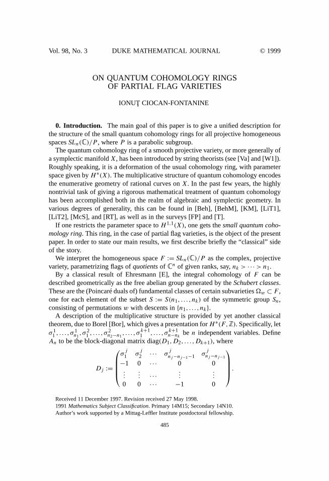
A description of the multiplicative structure is provided by yet another classicaltheorem, due to Borel [Bor], which gives a presentation forH ∗(F,Z). Specifically, letσ 1
1 , . . . ,σ1n1,σ 2
1 , . . . ,σ2n2−n1
, . . . ,σ k+11 , . . . ,σ k+1
n−nk be n independent variables. DefineAn to be the block-diagonal matrix diag(D1,D2, . . . ,Dk+1), where
Dj :=
σj
1 σj
2 · · · σj
nj−nj−1−1 σjnj−nj−1
−1 0 · · · 0 0...
... · · · ......
0 0 · · · −1 0
.Received 11 December 1997. Revision received 27 May 1998.1991Mathematics Subject Classification. Primary 14M15; Secondary 14N10.Author’s work supported by a Mittag-Leffler Institute postdoctoral fellowship.
485
486 IONUT CIOCAN-FONTANINE
Borel’s result states that there is a canonical isomorphism
Z[σ 1
1 , . . . ,σ1n1, . . . ,σ k+1
1 , . . . ,σ k+1n−nk
]/(g1,g2, . . . ,gn)∼=H ∗(F ),(0.1)
with g1, . . . ,gn the coefficients of the characteristic polynomial of the matrixAn.The natural problem arising from the above descriptions is to look for polynomial
representatives for the Schubert classes. The first case in which this problem wassolved is whenF is a Grassmannian, which goes back to Schur and Giambelli.
The general case was obtained independently by Bernstein, Gelfand, and Gelfand[BGG] and by Demazure [D]. In fact, it suffices to solve the above problem for thecompleteflag varietyFn = SLn(C)/B. The point is that the map
H ∗(F,Z)−→H ∗(Fn,Z)(0.2)
induced by flat pullback via the natural projectionFn → F is an embedding. Moreprecisely, the Borel description for the cohomology of the complete flag variety is
Z[x1,x2, . . . ,xn]/(e1, . . . ,en)∼=H ∗(Fn,Z),
whereej is the j th elementary symmetric polynomial inx1, . . . ,xn. A particularlynice set of representatives for the Schubert classes in this case is given by theSchubertpolynomialsSw(x1, . . . ,xn) of Lascoux and Schützenberger [LS]. If we interpret eachσji as theith elementary symmetric polynomial in variablesxnj−1+1, . . . ,xnj , then the
image ofH ∗(F,Z) by the map (0.2) is the subring of polynomials that are symmetricin variables in each of the groups
x1, . . . ,xn1︸ ︷︷ ︸,xn1+1, . . . ,xn2︸ ︷︷ ︸, . . . ,xnk+1, . . . ,xn︸ ︷︷ ︸ .If w ∈ S, thenSw satisfies the above symmetry; hence, it determines a polynomialPw in theσ variables, which represents[�w] in H ∗(F,Z). We call thePw(σ)’s theGiambelli polynomialsassociated toF . (WhenF is a Grassmannian, these are theGiambelli determinants in the Chern classes of the universal quotient.)
Within the Schubert varieties are thespecial Schubert varieties, which are geo-metric realizations of the Chern classes of the universal quotient bundles onF . Theycorrespond to the cyclic permutationsαi,j := snj−i+1× ·· · × snj , for 1≤ j ≤ k and1≤ i ≤ nj , wheresm := (m,m+1) is the simple transposition interchangingm andm+1. Again, whenF is a Grassmannian, there is a classical formula, due to Pieri,expressing the product[�αi,1] · [�w] in the basis of Schubert classes. Its generaliza-tion to the case of the complete flag variety, and hence, by the above discussion, toany partial flag variety as well, was first stated by Lascoux and Schützenberger [LS]and was given a geometric proof by Sottile [So].
In analogy to the case of Grassmannians, we refer to the Giambelli- and Pieri-typeformulas as theclassical Schubert calculusonF .
ON QUANTUM COHOMOLOGY RINGS OFSLn(C)/P 487
The small quantum cohomology ring ofF , denoted byQH ∗(F ), is defined as theZ[q1, . . . ,qk]-moduleH ∗(F,Z)⊗Z Z[q1, . . . ,qk], whereq1, . . . ,qk are formal vari-ables, with a new multiplication, which we denote by∗. This multiplication is ob-tained by replacing the classical structure constants with polynomials inq1, . . . ,qk,whose coefficients are the3-point, genus-zero Gromov-Witten (GW) invariantsof F .A presentation ofQH ∗(F )was given independently by Astashkevich and Sadov [AS]and by Kim [Kim1], with the proof completed in [Kim2]. (The “extreme” cases ofGrassmannians and complete flags were established slightly earlier in [ST], [W2] and[CF1], [GK], respectively.) Their result is as follows. LetBn = (blm)1≤l,m≤n be thematrix with entries
blm =
(−1)nj+1−nj+1qj , if l = nj−1+1 andm= nj+1, for 1≤ j ≤ k,−1, if l = nj +1 andm= nj , for 1≤ j ≤ k−1,
0, otherwise.
Then there exists a canonical isomorphism
Z[σ 1
1 , . . . ,σ1n1, . . . ,σ k+1
1 , . . . ,σ k+1n−nk
][q1, . . . ,qk
]/(G1, . . . ,Gn
)∼=QH ∗(F ),(0.3)
whereG1, . . . ,Gn are the coefficients of the characteristic polynomial of the deformedmatrixAqn := An+Bn.
From the point of view of enumerative geometry, one is interested in computingthe Gromov-Witten invariants ofF , and the description (0.3) is not too helpful unlessone has quantum versions of the Giambelli and Pieri formulas. In other words, oneis interested in developing aquantum Schubert calculus. The first such formulas, inthe case whereF is a Grassmannian, were discovered by Bertram, whose paper [Be]started the subject. Later, his approach was extended to the case of complete flagsto obtain the quantum Giambelli formula for thespecialSchubert classes (see [CF1]and [CF2]). Using this, thequantum Schubert polynomialswere constructed withalgebro-combinatorial methods by Fomin, Gelfand, and Postnikov [FoGP], thereforegiving the full quantum Giambelli formula for the variety of complete flags. They alsogave a special case of the quantum Pieri formula, namely, the quantum Monk formula,which corresponds to multiplying by thefirst Chern class of one of the tautologicalbundles.
As opposed to the situation of the classical cohomology, the quantum story for apartial flag variety is far from being determined by the one for the complete flags.The reason for this is that the quantum cohomology lacks the functoriality enjoyedby the usual one. The main results of this paper are general quantum versions of theGiambelli and Pieri formulas, which hold foranyF . These formulas specialize to theones mentioned above whenF is either a Grassmannian or the complete flag variety.In order to state them, we first introduce some notation.
488 IONUT CIOCAN-FONTANINE
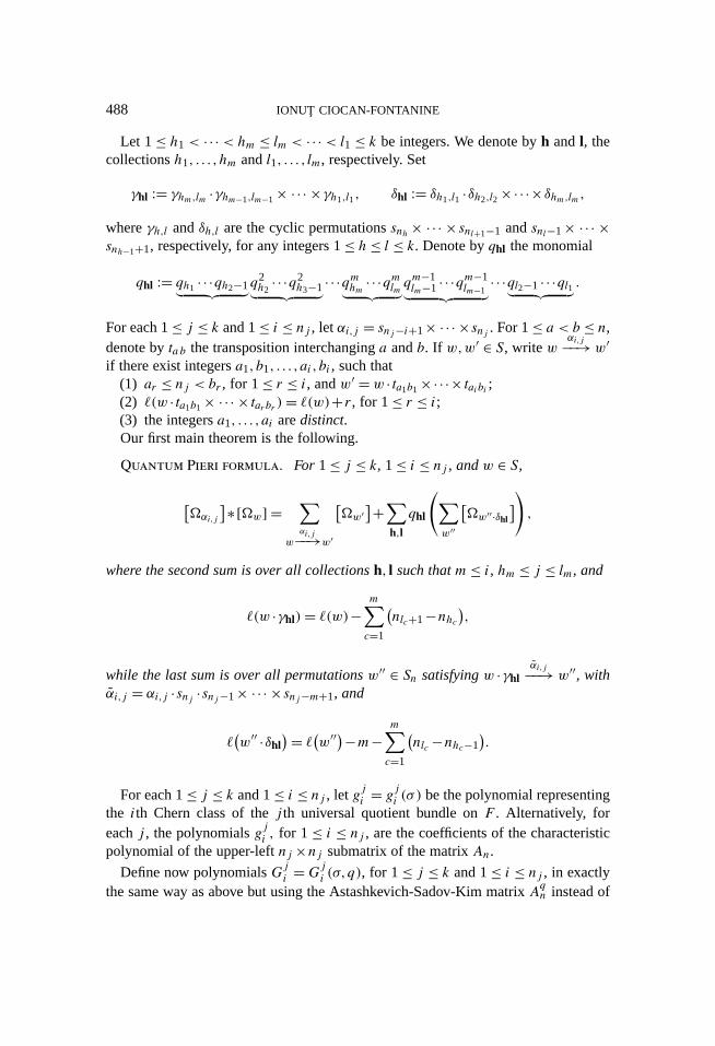
Let 1≤ h1 < · · · < hm ≤ lm < · · · < l1 ≤ k be integers. We denote byh and l, thecollectionsh1, . . . ,hm andl1, . . . , lm, respectively. Set
γhl := γhm,lm ·γhm−1,lm−1 × ·· · ×γh1,l1, δhl := δh1,l1 ·δh2,l2 ×·· ·×δhm,lm,whereγh,l andδh,l are the cyclic permutationssnh× ·· · × snl+1−1 andsnl−1× ·· · ×snh−1+1, respectively, for any integers 1≤ h≤ l ≤ k. Denote byqhl the monomial
lm−1︸ ︷︷ ︸ · · ·ql2−1 · · ·ql1︸ ︷︷ ︸ .For each 1≤ j ≤ k and 1≤ i ≤ nj , letαi,j = snj−i+1× ·· · ×snj . For 1≤ a < b ≤ n,denote byta b the transposition interchanginga andb. If w,w′ ∈ S, writew
αi,j−−→ w′if there exist integersa1,b1, . . . ,ai,bi , such that
(1) ar ≤ nj < br , for 1≤ r ≤ i, andw′ = w · ta1b1 ×·· ·× taibi ;(2) ((w · ta1b1 × ·· · × tarbr )= ((w)+r, for 1≤ r ≤ i;(3) the integersa1, . . . ,ai aredistinct.Our first main theorem is the following.
Quantum Pieri formula. For 1≤ j ≤ k, 1≤ i ≤ nj , andw ∈ S,
[�αi,j
]∗[�w] = ∑wαi,j−−→w′
[�w′
]+∑h,l
qhl
(∑w′′
[�w′′·δhl
]),
where the second sum is over all collectionsh, l such thatm≤ i, hm ≤ j ≤ lm, and
((w ·γhl)= ((w)−m∑c=1
(nlc+1−nhc
),
while the last sum is over all permutationsw′′ ∈ Sn satisfyingw ·γhl αi,j−−→ w′′, withαi,j = αi,j ·snj ·snj−1× ·· · ×snj−m+1, and
((w′′ ·δhl
)= ((w′′)−m−m∑c=1
(nlc−nhc−1
).
For each 1≤ j ≤ k and 1≤ i ≤ nj , let gji = gji (σ ) be the polynomial representingthe ith Chern class of thej th universal quotient bundle onF . Alternatively, foreachj , the polynomialsgji , for 1≤ i ≤ nj , are the coefficients of the characteristicpolynomial of the upper-leftnj ×nj submatrix of the matrixAn.
Define now polynomialsGji =Gji (σ,q), for 1≤ j ≤ k and 1≤ i ≤ nj , in exactlythe same way as above but using the Astashkevich-Sadov-Kim matrixA
qn instead of
ON QUANTUM COHOMOLOGY RINGS OFSLn(C)/P 489
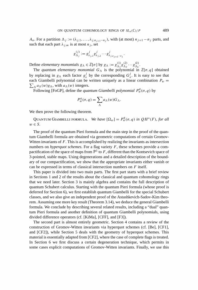
An. For a partition*j := (λj,1, . . . ,λj,nj+1−nj ), with (at most)nj+1−nj parts, andsuch that each partλj,m is at mostnj , set
g(j)*j
:= gjλj,1gjλj,2
· · ·gjλj,nj+1−nj.
Defineelementary monomialsg* ∈ Z[σ ] by g* := g(1)*1g(2)*2
· · ·g(k)*k .The quantum elementary monomialG* is the polynomial inZ[σ,q] obtained
by replacing ing* each factorgjλ by the correspondingGjλ. It is easy to see thateach Giambelli polynomial can be written uniquely as a linear combinationPw =∑*a*(w)g*, with a*(w) integers.Following [FoGP], define thequantum Giambelli polynomialPqw(σ,q) by
Pqw(σ,q)=∑*
a*(w)G*.
We then prove the following theorem.
Quantum Giambelli formula. We have[�w] = Pqw(σ,q) in QH ∗(F ), for allw ∈ S.
The proof of the quantum Pieri formula and the main step in the proof of the quan-tum Giambelli formula are obtained via geometric computations of certain Gromov-Witten invariants ofF . This is accomplished by realizing the invariants as intersectionnumbers onhyperquot schemes. For a flag varietyF , these schemes provide a com-pactification of the space of maps fromP1 toF , different than the Kontsevich space of3-pointed, stable maps. Using degenerations and a detailed description of the bound-ary of our compactification, we show that the appropriate invariants either vanish orcan be expressed in terms of classical intersection numbers onF itself.
This paper is divided into two main parts. The first part starts with a brief reviewin Sections 1 and 2 of the results about the classical and quantum cohomology ringsthat we need later. Section 3 is mainly algebra and contains the full description ofquantum Schubert calculus. Starting with the quantum Pieri formula (whose proof isdeferred for Section 6), we first establish quantum Giambelli for the special Schubertclasses, and we also give an independent proof of the Astashkevich-Sadov-Kim theo-rem. Assuming one more key result (Theorem 3.14), we deduce the general Giambelliformula. We conclude by describing several related results, including a “dual” quan-tum Pieri formula and another definition of quantum Giambelli polynomials, usingdivided difference operators (cf. [KiMa], [CFF], and [F3]).
The second part is almost entirely geometric. Section 4 contains a review of theconstruction of Gromov-Witten invariants via hyperquot schemes (cf. [Be], [CF1],and [CF2]), while Section 5 deals with the geometry of hyperquot schemes. Thismaterial is essentially adapted from [CF2], where the case of complete flags is treated.In Section 6 we first discuss a certain degeneration technique, which permits insome cases explicit computations of Gromov-Witten invariants. Finally, we use this
490 IONUT CIOCAN-FONTANINE
technique, together with the results in the previous two sections, to prove quantumPieri and complete the proof of quantum Giambelli, by establishing the key resultmentioned above.
Acknowledgements.I have learned the subject from Aaron Bertram, and manyof the ideas used in this paper originate in his work on quantum cohomology ofGrassmannians. I am indebted to William Fulton and Bumsig Kim for very usefuldiscussions during the preparation of the paper. This work was completed while Iparticipated in the 1996–1997 program “Enumerative Geometry and Its Relation withTheoretical Physics” at the Mittag-Leffler Institute. I am grateful to the organizers ofthe program and to the staff of the Institute for the stimulating research atmosphereprovided throughout the year.
1. The classical cohomology ring
1.1. Schubert varieties.Let 0= n0< n1< n2< · · ·< nk < nk+1 = n be integers.Let V be a complexn-dimensional vector space. The datak, nj , j = 0, . . . ,k+1,andV are fixed for the rest of the paper. DefineF := F(n1, . . . ,nk,V ) to be thevariety parametrizing flags ofquotientsof V , with ranks given by thenj ’s. F is asmooth, irreducible, projective variety, of dimensionf :=∑k
j=1(n−nj )(nj−nj−1).It comes with a tautological sequence of quotient bundles
VF := V ⊗�F �Qk �Qk−1 � · · · �Q1,
with rank(Qj )= nj .Let Sn be the symmetric group onn letters, and letS := S(n1, . . . ,nk) ⊂ Sn be
the subset consisting of permutationsw with descents in{n1, . . . ,nk}. In other words,when regarded as a function[1,n] → [1,n], w is increasing on each of the intervals[1,n1], [n1+1,n2], . . . , [nk+1,nk+1]. Therank functionof a permutationw ∈ Sn isdefined by
rw(q,p)= card{i | i ≤ q,w(i)≤ p}, for 1≤ q,p ≤ n.
Fix a complete flag of subspacesV1 ⊂ V2 ⊂ ·· · ⊂ Vn−1 ⊂ Vn = V . Forw ∈ S, thecorresponding Schubert variety is defined by
�w := {x ∈ F | rankx
(Vp⊗� →Qq
)≤ rw(q,p),q ∈ {n1, . . . ,nk},1≤ p ≤ n}.�w is an irreducible subvariety inF of (complex) codimension equal to the length((w) of the permutationw. Thedual Schubert varietyto�w is the Schubert varietycorresponding to the permutationw ∈ S, given by
w(i)= n−w(nj +nj−1− i+1)+1, for nj−1+1≤ i ≤ nj ,1≤ j ≤ k.
Throughout this paper,H ∗(F ) denotes the integral cohomology ofF . The fol-lowing two theorems are classical results of Ehresmann [E] (see also [F2, Example14.7.16]).
1.2. A presentation ofH ∗(F ). Consider onF the vector bundles
Lj := ker(Qj →Qj−1
),
and letσ ji := ci(Lj ), for 1 ≤ i ≤ nj − nj−1 and 1≤ j ≤ k + 1. Let x1, . . . ,xnbe independent variables. For all 0≤ i ≤ m ≤ n, let emi denote theith elementarysymmetric function in the variablesx1, . . . ,xm. We regard the variables in each of thegroups
x1, . . . ,xn1︸ ︷︷ ︸,xn1+1, . . . ,xn2︸ ︷︷ ︸, . . . ,xnk+1, . . . ,xn︸ ︷︷ ︸as the Chern roots of the bundlesQ1 andL2, . . . ,Lk+1, respectively. For each 1≤ j ≤k+1, the polynomialse
nji can be written as polynomialsgji = gji (σ 1
1 , . . . ,σk+1nk+1−nk )
in the Chern classes of these bundles. The polynomialgji has weighted degreei,
where eachσ ∗m is assigned degreem. In particular, we have polynomialsgk+1
i , for1≤ i ≤ n.
Denote the polynomial ringZ[σ 11 , . . . ,σ
1n1,σ 2
1 , . . . ,σ2n2−n1
, . . . ,σ k+11 , . . . ,σ k+1
n−nk ] byZ[σ ]. The following is another classical result, due to Borel [Bor].
Theorem 1.3. H ∗(F ) is canonically isomorphic toZ[σ ]/(gk+11 , . . . ,gk+1
n ).
1.3. Classical Schubert calculus forF . Let us recall the Schubert polynomialsof Lascoux and Schützenberger [LS]. Define operators∂i , for i = 1, . . . ,n− 1, onZ[x1, . . . ,xn] by
For anyw ∈ Sn, write w = w◦ · si1 × ·· ·× sik , with k = n(n−1)/2− ((w), wheresi = (i, i + 1) is the transposition interchangingi and i + 1, and wherew◦ is thepermutation of longest length, given byw◦(j) = n− j + 1, for 1 ≤ j ≤ n. TheSchubert polynomialSw(x) ∈ Z[x1, . . . ,xn] is defined by
Sw(x)= ∂ik ◦· · ·◦∂i1(xn−11 xn−2
2 · · ·xn−1).
It is shown in [M] that ifw ∈ S, then the corresponding Schubert polynomial issymmetric in each group of variables
hence, it can be written as a polynomialPw(σ) of weighted degree((w). We call thesePw(σ) Giambelli polynomials. The following theorem is due to Bernstein, Gelfand,and Gelfand [BGG] and Demazure [D].
Theorem 1.4 (Giambelli-type formula). [�w] = Pw(σ) in H ∗(F ).
In particular, consider the cyclic permutations (of lengthi) αi,j := snj−i+1× ·· · ×snj and βi,j := snj+i−1 × ·· · × snj . Note that these permutations are inS. Their
symmetric polynomial in variablesx1, . . . ,xnj . Let f ji (σ ) be the polynomial in the
σ -variables obtained fromhnji . By Theorem 1.4,[
�αi,j]= gji and
[�βi,j
]= f ji in H ∗(F ).(1.1)
The following Pieri-type formula, due to Lascoux and Schützenberger [LS], recentlywas given a geometric proof by Sottile [So].
Let w,w′ ∈ S. For 1≤ a < b ≤ n, denote bytab the transposition interchanginga
andb. Writewαi,j−−→ w′ if there exist integersa1,b1, . . . ,ai,bi , satisfying
(1) am ≤ nj < bm, for 1≤m≤ i, andw′ = w · ta1b1 × ·· · × taibi ;(2) ((w · ta1b1 × ·· · × tambm)= ((w)+m, for 1≤m≤ i; and
(3α) the integersa1, . . . ,ai aredistinct.
Similarly,wβi,j−−→ w′ if there exista1,b1, . . . ,ai,bi as above, satisfying (1), (2) and
(3β) b1, . . . ,bi aredistinct.
Theorem 1.5 (Pieri formula). The following hold inH ∗(F ):(i) [�αi,j ] · [�w] =
∑w
αi,j−−→w′[�w′ ];
(ii) [�βi,j ] · [�w] =∑w
βi,j−−→w′[�w′ ].
Remark 1.6. From the exact sequence
0−→ Lj −→Qj −→Qj−1 −→ 0,
we getci(Qj )=∑nj−nj−1r=0 σ
jr ci−r (Qj−1). But one easily sees thatci(Qj )= [�αi,j ].
Using (1.1), it follows that the polynomialsgji satisfy the following recursion (whichin fact defines them uniquely):
gji =
nj−nj−1∑r=0
σjr gj−1i−r ,(1.2)
where, by convention, we setgj−10 = 1 andgj−1
m = 0, if eitherm< 0 orm> nj−1.Also, using the same exact sequence, the relations (1.1) and (1.2), and the well-
known identity
ON QUANTUM COHOMOLOGY RINGS OFSLn(C)/P 493(nj−1∑r=0
enj−1r t r
)−1
=∑p≥0
(−1)phnj−1p tp,
we get that the following identities hold inH ∗(F ):
σjr =
r∑p=0
(−1)p[�βp,j−1
] ·[�αr−p,j ],(1.3)
[�αi,j
]= nj−nj−1∑r=0
r∑p=0
(−1)p[�βp,j−1
] ·[�αr−p,j ] ·[�αi−r,j−1
],(1.4)
where, by convention,[�α0,m] = [�β0,m] = 1 and[�α<0,m] = 0, for allm.
2. The small quantum cohomology ring ofF . We give below the precise def-inition of the small quantum cohomology ring only for the specific case of a partialflag manifold.
The 3-point, genus-zero Gromov-Witten (GW) invariantsof F , which we denoteby I3,β(γ1γ2γ3), are defined as intersection numbers on Kontsevich’s moduli spaceof stable mapsM0,3(F,β) (see [KM], [K], [BehM], and [FP]). Hereβ ∈H2(F ) andγ1,γ2,γ3 ∈ H ∗(F ). The enumerative significance of these numbers is given by thefollowing result, whose proof can be found in [FP, Lemma 14].
Lemma 2.1. Let51,52, and53 be closed subvarieties ofF representing the coho-mology classesγ1,γ2, andγ3, respectively. Letg1,g2,g3 ∈ SL(n,C) be general ele-ments, and denote bygi5i the translate of5i bygi . ThenI3,β(γ1γ2γ3) is the numberof mapsµ : P1 → F such thatµ∗[P1] = β andµ(P1) meetsg151,g252, andg353.
Since we give a different construction of these invariants in Section 4, we shallsay no more about them here. The multiplication in the (small) quantum cohomologyring is defined using theseI3,β as structure constants. More precisely, this goes asfollows.
Introduce formal variablesq1, . . . ,qk, corresponding, respectively, to the generators(cf. Theorem 1.1)[�sn1 ], . . . , [�snk ] ofH2(F ). For a (holomorphic) mapµ : P1 → F ,
we can writeβ = µ∗[P1] = ∑kj=1dj [�snj ], with dj nonnegative integers. We say
thatµ has multidegreed = (d1, . . . ,dk), and we replaceβ by d in the notation forGW invariants.
LetK := Z[q1, . . . ,qk]. On theK-moduleH ∗(F )⊗ZK, define the quantum mul-tiplication ∗ by putting first[
�u]∗[�v] :=∑
d
qd11 · · ·qdkk
∑w∈S
I3,d
([�u][�v][�w
])[�w
],(2.1)
for all u,v ∈ S, and then extending linearly onH ∗(F ) and trivially onK. The
494 IONUT CIOCAN-FONTANINE
following theorem is a particular case of the general results on associativity of quan-tum cohomology (see [Beh], [BehM], [KM], [LiT1], [LiT2], [McS], and [RT]).
Theorem 2.2. The operation∗ defines an associative and commutativeK-algebrastructure onH ∗(F )⊗ZK.
H ∗(F )⊗ZK together with this multiplication is called the small quantum coho-mology ring ofF and is denoted byQH ∗(F ). The goal of this paper is to give adescription analogous to that in Section 1 for this new algebra.
3. Quantum Schubert calculus
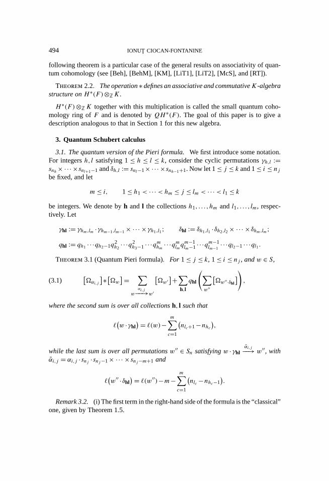
3.1. The quantum version of the Pieri formula.We first introduce some notation.For integersh, l satisfying 1≤ h ≤ l ≤ k, consider the cyclic permutationsγh,l :=snh× ·· · ×snl+1−1 andδh,l := snl−1× ·· · ×snh−1+1. Now let 1≤ j ≤ k and 1≤ i ≤ njbe fixed, and let
m≤ i, 1≤ h1< · · ·< hm ≤ j ≤ lm < · · ·< l1 ≤ kbe integers. We denote byh and l the collectionsh1, . . . ,hm and l1, . . . , lm, respec-tively. Let
Theorem 3.1 (Quantum Pieri formula). For 1≤ j ≤ k, 1≤ i ≤ nj , andw ∈ S,[�αi,j
]∗[�w]= ∑w
αi,j−−→w′
[�w′
]+∑h,l
qhl
(∑w′′
[�w′′·δhl
]),(3.1)
where the second sum is over all collectionsh, l such that
((w ·γhl
)= ((w)− m∑c=1
(nlc+1−nhc
),
while the last sum is over all permutationsw′′ ∈ Sn satisfyingw ·γhl αi,j−−→ w′′, withαi,j = αi,j ·snj ·snj−1× ·· · ×snj−m+1 and
((w′′ ·δhl
)= ((w′′)−m−m∑c=1
(nlc−nhc−1
).
Remark 3.2. (i) The first term in the right-hand side of the formula is the “classical”one, given by Theorem 1.5.
ON QUANTUM COHOMOLOGY RINGS OFSLn(C)/P 495
(ii) The condition((w ·γhl)= ((w)−∑mc=1(nlc+1−nhc) can be rephrased equiva-
lently as
w(nhc)>max
{w(nhc+1), . . . ,w(nlc+1)
}, for 1≤ c ≤m.(∗)
(iii) Note that if m < i, then αi,j = snj−i+1× ·· · × snj−m gives the same kindof cyclic permutation asαi,j , but it determines a Schubert variety only on the flagvarieties for which one of the quotients has ranknj −m! In fact, as seen in the proofof Theorem 3.1, the last sum in the formula comes from applying Theorem 1.5 onsuch a flag variety. That is, the permutationsw′′ are obtained from the terms in the“classical Pieri” for the multiplication of Schubert varieties corresponding tow ·γhlandαi,j . However, it can be easily checked that the permutationsw′′ ·δhl are in fact inS; hence, they define Schubert varieties on our originalF(n1, . . . ,nk,V ). (If m = i,then αi,j is the identity permutation.) Also note that for the terms appearing in thelast sum, we have
((w′′ ·δhl
)= ((w)+ i− m∑c=1
(nlc−nhc−1
)− m∑c=1
(nlc+1−nhc
)= ((w)+((αi,j )−deg(qhl).
(iv) Although the formula seems rather complicated, it is in fact fairly easy tocompute, using the following four steps:
(1) decide which monomialsqhl may appear (these are determined byi andj , dueto the conditionsm≤ i andhm ≤ j ≤ lm);
(2) discard allh, l for which the condition(∗) in Remark 3.2(ii) above is notsatisfied;
(3) for each of the remaining collectionsh, l, perform the classical Pieri multipli-cation of[�w·γhl ] and[�αi,j ];
(4) finally, multiply (to the right) the permutationsw′′ obtained in the previousstep byδhl and discard all the ones for which the length does not drop by thenumber of factors inδhl .
For example, ifF = F(1,3,4,C5), w = (53421) (the corresponding Schubert classis the class of a point), andα2,2 = (13425) is the cycle giving the second Chern classof the tautological quotient bundle of rank 3 onF , one computes[
�(13425)]∗[�(53421)
]= q2[�(52431)]+q1q2[�(23541)
]+q2q3[�(51423)]
+q1q2q3[�(13524)
]+q1q22q3
[�(12345)
].
(v) In the case whenF is thecompleteflag variety, a quantum Pieri formula isstated in the recent preprint [KiMa] of Kirillov and Maeno, and an algebraic proof issuggested. Their formulation is quite different, and we have not checked to see if itagrees with what Theorem 3.1 says in that case.
496 IONUT CIOCAN-FONTANINE
Another quantum Pieri formula, due to Lascoux and Veigneau (only for completeflags and only with an algebraic proof suggested), is announced in [Ve]. The formu-lation is different, but it can be seen to agree with Theorem 3.1.
After this paper was completed, Postnikov [Po] gave an algebro-combinatorialproof of quantum Pieri for complete flags, in yet another different but equivalentformulation.
We prove Theorem 3.1 in Section 6. For the moment, let us see what it says insome special cases, namely,Grassmannians, complete flag varieties, and Lemmas 3.5and 3.6.
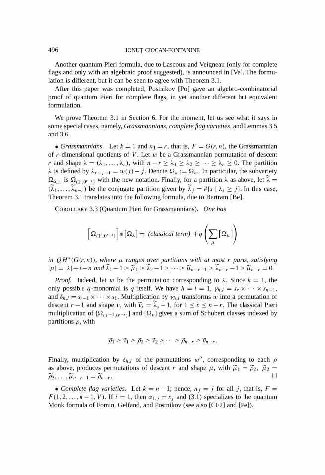
• Grassmannians.Let k = 1 andn1 = r, that is,F =G(r,n), the Grassmannianof r-dimensional quotients ofV . Let w be a Grassmannian permutation of descentr and shapeλ = (λ1, . . . ,λr), with n− r ≥ λ1 ≥ λ2 ≥ ·· · ≥ λr ≥ 0. The partitionλ is defined byλr−j+1 = w(j)− j . Denote�λ := �w. In particular, the subvariety�αi,1 is �(1i ,0r−i ) with the new notation. Finally, for a partitionλ as above, letλ =(λ1, . . . , λn−r ) be the conjugate partition given byλj = #{s | λs ≥ j}. In this case,Theorem 3.1 translates into the following formula, due to Bertram [Be].
Corollary 3.3 (Quantum Pieri for Grassmannians). One has
[�(1i ,0r−i )
]∗[�λ]= (classical term)+q
(∑µ
[�µ])
in QH ∗(G(r,n)), whereµ ranges over partitions with at mostr parts, satisfying|µ| = |λ|+ i−n and λ1−1≥ µ1 ≥ λ2−1≥ ·· · ≥ µn−r−1 ≥ λn−r−1≥ µn−r = 0.
Proof. Indeed, letw be the permutation corresponding toλ. Sincek = 1, theonly possibleq-monomial isq itself. We haveh = l = 1, γh,l = sr × ·· · × sn−1,andδh,l = sr−1× ·· · ×s1. Multiplication byγh,l transformsw into a permutation ofdescentr−1 and shapeν, with νs = λs −1, for 1≤ s ≤ n− r. The classical Pierimultiplication of [�(1i−1,0r−i )] and[�ν] gives a sum of Schubert classes indexed bypartitionsρ, with
ρ1 ≥ ν1 ≥ ρ2 ≥ ν2 ≥ ·· · ≥ ρn−r ≥ νn−r .
Finally, multiplication by δh,l of the permutationsw′′, corresponding to eachρas above, produces permutations of descentr and shapeµ, with µ1 = ρ2, µ2 =ρ3, . . . , µn−r−1 = ρn−r .
• Complete flag varieties.Let k = n−1; hence,nj = j for all j , that is,F =F(1,2, . . . ,n−1,V ). If i = 1, thenα1,j = sj and (3.1) specializes to the quantumMonk formula of Fomin, Gelfand, and Postnikov (see also [CF2] and [Pe]).
ON QUANTUM COHOMOLOGY RINGS OFSLn(C)/P 497
Corollary 3.4 (Quantum Monk formula). One has inQH ∗(F )[�sj
]∗[�w] = (classical term)+∑thl
qh · · ·ql−1[�w·thl
],
where the sum is over all transpositions of integersh, l, with1≤ h≤ j < l ≤ n, suchthat ((w · thl)= ((w)−2(l−h)+1.
Finally, we now look closer at a special case, which is needed later. Recall theidentity (1.4), which holds in the classical cohomology ring of our partial flag variety:
[�αi,j
]= nj−nj−1∑r=0
r∑p=0
(−1)p[�βp,j−1
] ·[�αr−p,j ] ·[�αi−r,j−1
].
We want to compute the right-hand side when the classical product is replaced bythe quantum product. Of course, the answer is obtained by applying Theorem 3.1twice, but this would seem to give, besides the classical term[�αi,j ], numerous“quantum correction” terms. In fact, a more careful analysis shows that there is eitherno correction term or only one such term that we explicitly identify. It is better tobreak the computation into two pieces.
Lemma 3.5. (i) In the classical cohomology ringH ∗(F ), we have, for0 ≤ p ≤r ≤ nj −nj−1, [
�βp,j−1
] ·[�αr−p,j ]= [�βp,j−1·αr−p,j
].
(ii) In the quantum cohomology ringQH ∗(F ), we have[�βp,j−1
]∗[�αr−p,j ]= [�βp,j−1·αr−p,j
]as well; that is, there are no quantum correction terms.
Proof. (i) This is a straightforward computation, for example, using Theorem 1.5(Sottile’s theorem).
(ii) Pick 1≤ h1 < · · · < hm ≤ j ≤ lm < · · · < l1 ≤ k. Sincenj ≥ r+nj−1 ≥ p+nj−1, we also havenl1+1 ≥ nj+1 ≥ nj+1≥ nj−1+p+1. Therefore,βp,j−1(nl1+1) >
βp,j−1(m), for all m< nl1+1, by the definition ofβp,j−1. In particular,
βp,j−1(nl1+1
)> βp,j−1
(nh1
).(3.2)
To get a quantum contribution for the chosenhi andli , we should have, necessarily,by Remark 3.2(ii),
βp,j−1(nh1
)>max
{βp,j−1
(nh1 +1
), . . . ,βp,j−1
(nl1+1
)}.
This contradicts (3.2).
498 IONUT CIOCAN-FONTANINE
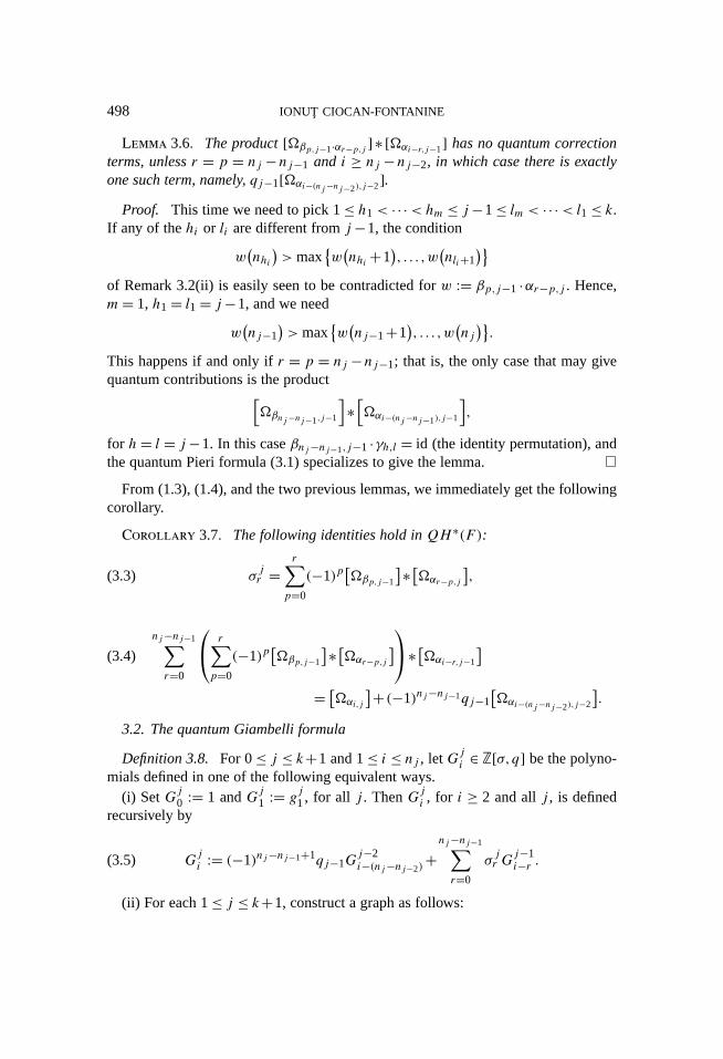
Lemma 3.6. The product[�βp,j−1·αr−p,j ] ∗ [�αi−r,j−1] has no quantum correctionterms, unlessr = p = nj −nj−1 and i ≥ nj −nj−2, in which case there is exactlyone such term, namely,qj−1[�αi−(nj−nj−2),j−2].
Proof. This time we need to pick 1≤ h1< · · ·< hm ≤ j−1≤ lm < · · ·< l1 ≤ k.If any of thehi or li are different fromj−1, the condition
w(nhi)>max
{w(nhi +1
), . . . ,w
(nli+1
)}of Remark 3.2(ii) is easily seen to be contradicted forw := βp,j−1 ·αr−p,j . Hence,m= 1, h1 = l1 = j−1, and we need
w(nj−1
)>max
{w(nj−1+1
), . . . ,w
(nj)}.
This happens if and only ifr = p = nj −nj−1; that is, the only case that may givequantum contributions is the product[
�βnj−nj−1,j−1
]∗[�αi−(nj−nj−1),j−1
],
for h= l = j−1. In this caseβnj−nj−1,j−1 ·γh,l = id (the identity permutation), andthe quantum Pieri formula (3.1) specializes to give the lemma.
From (1.3), (1.4), and the two previous lemmas, we immediately get the followingcorollary.
Corollary 3.7. The following identities hold inQH ∗(F ):
σjr =
r∑p=0
(−1)p[�βp,j−1
]∗[�αr−p,j ],(3.3)
(3.4)
nj−nj−1∑r=0
r∑p=0
(−1)p[�βp,j−1
]∗[�αr−p,j ]∗[�αi−r,j−1
]= [�αi,j
]+(−1)nj−nj−1qj−1[�αi−(nj−nj−2),j−2
].
3.2. The quantum Giambelli formula
Definition 3.8. For 0≤ j ≤ k+1 and 1≤ i ≤ nj , letGji ∈ Z[σ,q] be the polyno-mials defined in one of the following equivalent ways.
(i) SetGj0 := 1 andGj1 := gj1, for all j . ThenGji , for i ≥ 2 and allj , is definedrecursively by
Gji := (−1)nj−nj−1+1qj−1G
j−2i−(nj−nj−2)
+nj−nj−1∑r=0
σjr G
j−1i−r .(3.5)
(ii) For each 1≤ j ≤ k+1, construct a graph as follows:
ON QUANTUM COHOMOLOGY RINGS OFSLn(C)/P 499
• choosej vertices and label themv1, . . . ,vj ;• for every 1≤ l ≤ j−1, join the verticesvl andvl+1 by an edge and give it the
label(−1)nl+1−nl+1ql ;• for every 1≤ l ≤ j , attachnl −nl−1 tails to the vertexvl , with labelsσ l1, . . . ,σ lnl−nl−1
, respectively.
Now defineGji to be the sum of all monomials obtained by choosing edges inthis graph and forming the product of their labels, such that the total degree of themonomial isi, where deg(ql)= nl+1−nl−1 and deg(σ lm)=m, for everyl,m, and notwo of the chosen edges share a common vertex. This description was shown to meby W. Fulton.
(iii) For eachj , the polynomialsGji , for 1 ≤ i ≤ nj , are the coefficients of thecharacteristic polynomial det(Aqnj+λI), whereAqnj is the upper leftnj×nj submatrixof the Astashkevich-Sadov-Kim matrixAqn (see [AS], [Kim1], and [Kim2]).
It is immediate from any of these descriptions thatGji (σ,0)= gji (σ ). We are now
ready to formulate a special case of the quantum Giambelli formula.
Theorem 3.9. (i) [�αi,j ] = Gji (σ,q) in QH ∗(F ), for all 1 ≤ i ≤ nj and 0 ≤j ≤ k.
(ii) Gk+1i (σ,q)= 0 in QH ∗(F ), for all 1≤ i ≤ n.
Proof. The theorem follows by induction onj , using the identities (3.3) and (3.4)in Corollary 3.7, and the recursion (3.5) satisfied by theGji ’s.
Corollary 3.10 [AS], [Kim1], and [Kim2]. There is a canonical isomorphism
QH ∗(F )∼= Z[σ,q]/Iq,whereIq is the ideal(Gk+1
1 , . . . ,Gk+1n ).
Proof. This follows from Theorem 3.9(ii) and [ST, Theorem 2.2].
Remark 3.11.Theorem 3.9(ii) and Corollary 3.10 were formulated independentlyby Astashkevich and Sadov [AS] and Kim [Kim1], with the proof completed in[Kim2]. As far as I know, Theorem 3.9(i) is new here. For the case of complete flags,Theorem 3.9 and Corollary 3.10 were first proved in [CF1].
We now construct the polynomials that give the general quantum Giambelli for-mula, using an idea of Fomin, Gelfand, and Postnikov [FoGP]. For a partition*j :=(λj,1, . . . ,λj,nj+1−nj ) with (at most)nj+1−nj parts and such that each partλj,m isat mostnj , set
g(j)*j
:= gjλj,1gjλj,2
· · ·gjλj,nj+1−nj.
Defineelementary monomialsg* := g*1*2···*k ∈ Z[σ ] by
g* := g(1)*1g(2)*2
· · ·g(k)*k .(3.6)
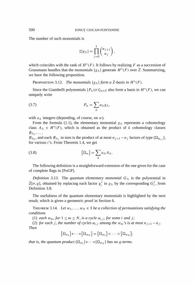
500 IONUT CIOCAN-FONTANINE
The number of such monomials is
<{g*} =k∏j=0
(nj+1
nj
),
which coincides with the rank ofH ∗(F ). It follows by realizingF as a succession ofGrassmann bundles that the monomials{g*} generateH ∗(F ) overZ. Summarizing,we have the following proposition.
Proposition 3.12. The monomials{g*} form aZ-basis inH ∗(F ).
Since the Giambelli polynomials{Pw(σ)}w∈S also form a basis inH ∗(F ), we canuniquely write
Pw =∑*
a*g*,(3.7)
with a* integers (depending, of course, onw).From the formula (1.1), the elementary monomialg* represents a cohomology
classA* ∈ H ∗(F ), which is obtained as the product ofk cohomology classesB*1, . . . ,
B*k , and eachB*j in turn is the product of at mostnj+1−nj factors of type[�αi,j ],for variousi’s. From Theorem 1.4, we get[
�w]=∑
*
a*A*.(3.8)
The following definition is a straightforward extension of the one given for the caseof complete flags in [FoGP].
Definition 3.13. The quantum elementary monomialG* is the polynomial inZ[σ,q], obtained by replacing each factorgji in g* by the correspondingGji , fromDefinition 3.8.
The usefulness of the quantum elementary monomials is highlighted by the nextresult, which is given a geometric proof in Section 6.
Theorem 3.14. Letw1, . . . ,wN ∈ S be a collection of permutations satisfying theconditions
(1) eachwm, for 1≤m≤N , is a cycleαi,j , for somei andj ;(2) for eachj , the number of cyclesαi,j among thewm’s is at mostnj+1−nj .
Then [�w1
]∗· · ·∗[�wN ]= [�w1
]× ·· · ×[�wN ];that is, the quantum product[�w1]∗ · · ·∗[�wN ] has noq-terms.
ON QUANTUM COHOMOLOGY RINGS OFSLn(C)/P 501
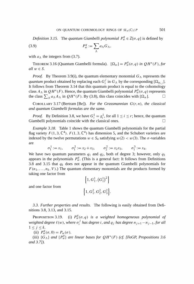
Definition 3.15. Thequantum Giambelli polynomialPqw ∈ Z[σ,q] is defined by
Pqw :=∑*
a*G*,(3.9)
with a* the integers from (3.7).
Theorem 3.16 (Quantum Giambelli formula). [�w] = Pqw(σ,q) in QH ∗(F ), forall w ∈ S.
Proof. By Theorem 3.9(i), the quantum elementary monomialG* represents thequantumproduct obtained by replacing eachGji in G* by the corresponding[�αi,j ].It follows from Theorem 3.14 that this quantum product is equal to the cohomologyclassA* inQH ∗(F ). Hence, the quantum Giambelli polynomialPqw(σ,q) representsthe class
∑*a*A* in QH ∗(F ). By (3.8), this class coincides with[�w].
Corollary 3.17 (Bertram [Be]). For the GrassmannianG(r,n), the classicaland quantum Giambelli formulas are the same.
Proof. By Definition 3.8, we haveG1i = g1
i , for all 1≤ i ≤ r; hence, the quantumGiambelli polynomials coincide with the classical ones.
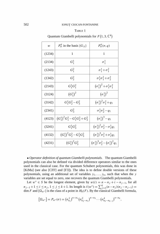
Example 3.18.Table 1 shows the quantum Giambelli polynomials for the partialflag varietyF(1,3,C4). F(1,3,C4) has dimension 5, and the Schubert varieties areindexed by the twelve permutationsw ∈ S4 satisfyingw(2) < w(3). Theσ -variablesare
σ 11 := x1, σ 2
1 := x2+x3, σ 22 := x2x3, σ 3
1 := x4.We have two quantum parametersq1 and q2, both of degree 3; however, onlyq1appears in the polynomialsPqw. (This is a general fact: It follows from Definitions3.8 and 3.15 thatqk does not appear in the quantum Giambelli polynomials forF(n1, . . . ,nk,V ).) The quantum elementary monomials are the products formed bytaking one factor from {
1,G11,(G1
1
)2}and one factor from {
1,G21,G
22,G
23
}.
3.3. Further properties and results.The following is easily obtained from Defi-nitions 3.8, 3.13, and 3.15.
Proposition 3.19. (i) Pqw(σ,q) is a weighted homogeneous polynomial ofweighted degree((w), whereσ ji has degreei, andqj has degreenj+1−nj−1, for all1≤ j ≤ k.
(ii) Pqw(σ,0)= Pw(σ).(iii) {G*} and {Pqw} are linear bases forQH ∗(F ) (cf. [FoGP, Propositions 3.6
and 3.7]).
502 IONUT CIOCAN-FONTANINE
Table 1
Quantum Giambelli polynomials forF(1,3,C4
)w P
qw in the basis{G*} P
qw(σ,q)
(1234) 1 1
(2134) G11 σ 1
1
(1243) G21 σ 1
1+σ 21
(1342) G22 σ 1
1σ21+σ 2
2
(2143) G11G
21
(σ 1
1
)2+σ 11σ
21
(3124)(G1
1
)2 (σ 1
1
)2(3142) G1
1G22−G2
3
(σ 1
1
)2σ 2
1+q1(2341) G2
3 σ 11σ
22−q1
(4123)(G1
1
)2G2
1−G11G
22+G2
3
(σ 1
1
)3−q1(3241) G1
1G23
(σ 1
1
)2σ 2
2−σ 11q1
(4132)(G1
1
)2G2
2−G11G
23
(σ 1
1
)3σ 2
1+σ 11q1
(4231)(G1
1
)2G2
3
(σ 1
1
)3σ 2
2−(σ 1
1
)2q1
• Operator definition of quantum Giambelli polynomials.The quantum Giambellipolynomials can also be defined via divided difference operators similar to the onesused in the classical case. For the quantum Schubert polynomials, this was done in[KiMa] (see also [CFF] and [F3]). The idea is to define double versions of thesepolynomials, using an additional set of variablesy1, . . . ,yn, such that when theyvariables are set equal to zero, one recovers the quantum Giambelli polynomials.
Let w◦ ∈ S be the longest element, given byw(i) = n− nj + i − nj−1, for allnj−1+1≤ i ≤ nj , 1≤ j ≤ k+1. Its length is((w◦)=∑k
j=1(n−nj )(nj −nj−1)=dimF and[�w◦ ] is the class of a point inH0(F ). By the classical Giambelli formula,[
�w◦]= Pw◦(σ )= (
σ 1n1
)n−n1(σ 2n2−n1
)n−n2 · · ·(σknk−nk−1
)n−nk ,
ON QUANTUM COHOMOLOGY RINGS OFSLn(C)/P 503
while expressing[�w◦ ] in the basis{g*} yields[�w◦
]= g1n1g1n1· · ·g1
n1︸ ︷︷ ︸n2−n1 factors
g2n2g2n2· · ·g2
n2︸ ︷︷ ︸n3−n2 factors
· · ·gknkgknk · · ·gknk︸ ︷︷ ︸nk+1−nk factors
= g*◦,
where
*◦ = (*1, . . . ,*k
), *j = (nj , . . . ,nj︸ ︷︷ ︸)
nj+1−nj terms
.
For all integersm, and allj ∈ {1,2, . . . ,k}, set
fm(j) :=m∑r=0
(−1)rGjm−rhr(yn−nj+1+1, . . . ,yn−nj
),
whereGji = Gji (σ,q) are the polynomials in Definition 3.8 fori ≤ nj , Gji = 0 fori > nj , andhr(yn−nj+1+1, . . . ,yn−nj ) is therth complete symmetric function in theindicated variables. Now set
D(j) := det(fnj+b−a(j)
)1≤a,b≤nj+1−nj ,
and define thequantum double Giambelli polynomial ofw◦ to be
Pw◦(σ,q,y) :=k∏j=1
D(j).
For 1≤ l ≤ n, ∂yl denotes the divided difference operator acting on polynomialsP(σ,q,y) by
∂yl P (σ,q,y)=
P(σ,q,y)−syl P (σ,q,y)yl+1−yl ,
with the operatorsyl interchangingyl andyl+1.For every permutationw ∈ S, one can writew = slt × ·· · × sl1 ·w◦, with t =
((w◦)−((w). We define thequantum double Giambelli polynomialPw(σ,q,y) by
Pw(σ,q,y) := (−1)t ∂ylt ◦· · ·◦∂yl1
(Pw◦(σ,q,y)
).
A proof of the next proposition can be found in [F3, Section 4] (cf. [KiMa], [CFF]).
Proposition 3.20. The polynomialPw(σ,q,0) coincides with the quantumGiambelli polynomialPqw in Definition 3.15.
504 IONUT CIOCAN-FONTANINE
• Orthogonality. For a polynomialR ∈ Z[σ ], consider the expansion of its cosetR(modI ) ∈ Z[σ ]/I in the basis{Pw} and define
〈R〉 := coefficient ofPw◦ .
Alternately, expandR(modI ) in the basis{g*} and take the coefficient ofg*◦ . Bythe classical Giambelli formula (Theorem 1.3), we can reformulate Theorem 1.2 asthe following.
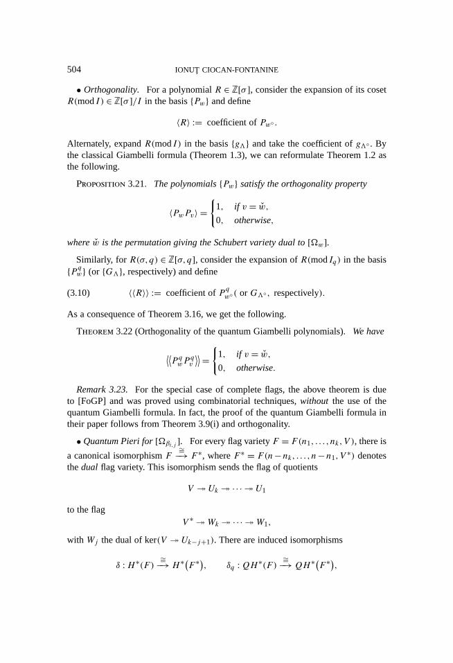
Proposition 3.21. The polynomials{Pw} satisfy the orthogonality property
〈PwPv〉 ={
1, if v = w,0, otherwise,
wherew is the permutation giving the Schubert variety dual to[�w].Similarly, forR(σ,q) ∈ Z[σ,q], consider the expansion ofR(modIq) in the basis
As a consequence of Theorem 3.16, we get the following.
Theorem 3.22 (Orthogonality of the quantum Giambelli polynomials). We have
⟨⟨PqwP
qv
⟩⟩= {1, if v = w,0, otherwise.
Remark 3.23.For the special case of complete flags, the above theorem is dueto [FoGP] and was proved using combinatorial techniques,without the use of thequantum Giambelli formula. In fact, the proof of the quantum Giambelli formula intheir paper follows from Theorem 3.9(i) and orthogonality.
• Quantum Pieri for[�βi,j ]. For every flag varietyF = F(n1, . . . ,nk,V ), there is
a canonical isomorphismF∼=−→ F ∗, whereF ∗ = F(n−nk, . . . ,n−n1,V
∗) denotesthedual flag variety. This isomorphism sends the flag of quotients
V � Uk � · · · � U1
to the flagV ∗ �Wk � · · · �W1,
with Wj the dual of ker(V � Uk−j+1). There are induced isomorphisms
δ :H ∗(F )∼=−→H ∗(F ∗), δq :QH ∗(F )
∼=−→QH ∗(F ∗),
ON QUANTUM COHOMOLOGY RINGS OFSLn(C)/P 505
on the classical and quantum cohomology rings. The mapδq acts on the Schubertbasis byδq([�w])= [�w◦ww◦ ] and on theq variables byδq(qj )= qk−j . (Recall thatw◦ is the longest permutation in the symmetric groupSn, given byw◦(i)= n−i+1.)In particular, one getsδq([�βi,j ])= [�αi,k−j+1].
Hence, in complete analogy with the classical case, the Pieri formula for quantummultiplication with the classes[�αi,j ] onF ∗ (Theorem 3.1) gives a formula for quan-tum multiplication with the classes[�βi,j ] onF . The proofs of the above statements,as well as writing down the actual formula, are straightforward and left to the reader.
We have completed the description ofQH ∗(F ), modulo the proofs of Theorems3.1 and 3.14. The last three sections of the paper are devoted to these proofs, whichare based on the geometry of compactifications of spaces of mapsP1 → F givenby hyperquot schemes. Most of the arguments in [CF2], where the case of completeflags is treated, require little or no changes. Therefore, we refer to the correspondingresults in [CF2] when appropriate and give details only as needed.
4. GW invariants via hyperquot schemes.We recall in this section the construc-tion of 3-point, genus-zero GW invariants by means of hyperquot schemes. Detailscan be found in [Be] and [CF2].
4.1. Hom and hyperquot schemes.For fixed d = (d1,d2, . . . ,dk), let Hd :=Homd(P
1,F ) be the moduli space of holomorphic mapsµ : P1 → F of multide-greed; that is, such thatµ∗[P1] =∑k
j=1dj [�snj ]. Hd is a quasi-projective scheme,
as it can be embedded as an open subscheme of the Hilbert scheme ofP1 × F .SinceF is a homogeneous space,H 1(P1,µ∗TF )= 0 for every mapµ, and standarddeformation theory shows thatHd is smooth and of dimension
h0(P1,µ∗TF)= dimF −µ∗
[P1] ·(KF )
=k∑j=1
(n−nj
)(nj −nj−1
)+ k∑j=1
dj(nj+1−nj−1
).
To give a map of multidegreed is equivalent to specifying a sequence of quotientbundles
VP1 �Mk � · · · �M1,
with rankMj = nj and deg(Mj )= dj , or, by dualizing, a sequence of subbundles
S1 ⊂ ·· · ⊂ Sk ⊂ V ∗P1,
with rankSj = nj and deg(Sj ) = −dj . Let Tj := V ∗P1/Sk−j+1. The Hilbert polyno-
mial of Tj is Pj (m)= (m+1)(n−nk−j+1)+dk−j+1.Let ��d := ��P1,...,Pk (P
1,V ∗P1) be the hyperquot scheme parametrizing flagged
sequences of quotientsheavesof V ∗P1, with Hilbert polynomials given byP1, . . . ,Pk.
506 IONUT CIOCAN-FONTANINE
Theorem 4.1 [Lau], [CF2], and [Kim3]. (i) ��d is a smooth, irreducible, projec-tive variety, of dimension
k∑j=1
(n−nj
)(nj −nj−1
)+ k∑j=1
dj(nj+1−nj−1
),
containingHd as an open dense subscheme.(ii) ��d is a fine moduli space; that is, there exists a universal sequence
V ∗P1×��d
� �dk � · · · � �d2 � �d1 � 0(†)
on P1��d such that each�dj is flat over��d , with relative Hilbert polynomialPj (m). The sequence has the property that for every schemeX overC, together witha sequence of quotients
V ∗P1×X �Qk � · · · �Q1(††)
such that eachQj is flat overX, with relative Hilbert polynomialPj , there exists aunique morphismCX : X→ ��d such that sequence (††) is the pullback of (†) via(id,CX).
(iii) Let �dj := ker(V ∗P1×��d
→ �dk−j+1). Then�dj is a vector bundleof ranknj
and relative degree−dj onP1×��d .
4.2. Generalized Schubert varieties onHd and��d . The moduli space of mapscomes with a universal evaluation morphism
ev: P1×Hd → F,
given byev(t, [µ])= µ(t), which can be used to pull back Schubert varieties toHd .More precisely, fort ∈ P1 andw ∈ S, define a subscheme ofHd by
�w(t)= ev−1(�w)⋂({t}×Hd).As a set,�w(t) consists of all maps of multidegreed, sendingt ∈ P1 to�w.
Alternately, the pullback�w(t) of a Schubert variety can be described as thedegeneracy locus{
where theQj ’s are the tautological quotient bundles onF and whereV1 ⊂ ·· · ⊂Vn−1 ⊂ Vn = V is our fixed reference flag. This last description may be used toextend�w(t) to ��d .
ON QUANTUM COHOMOLOGY RINGS OFSLn(C)/P 507
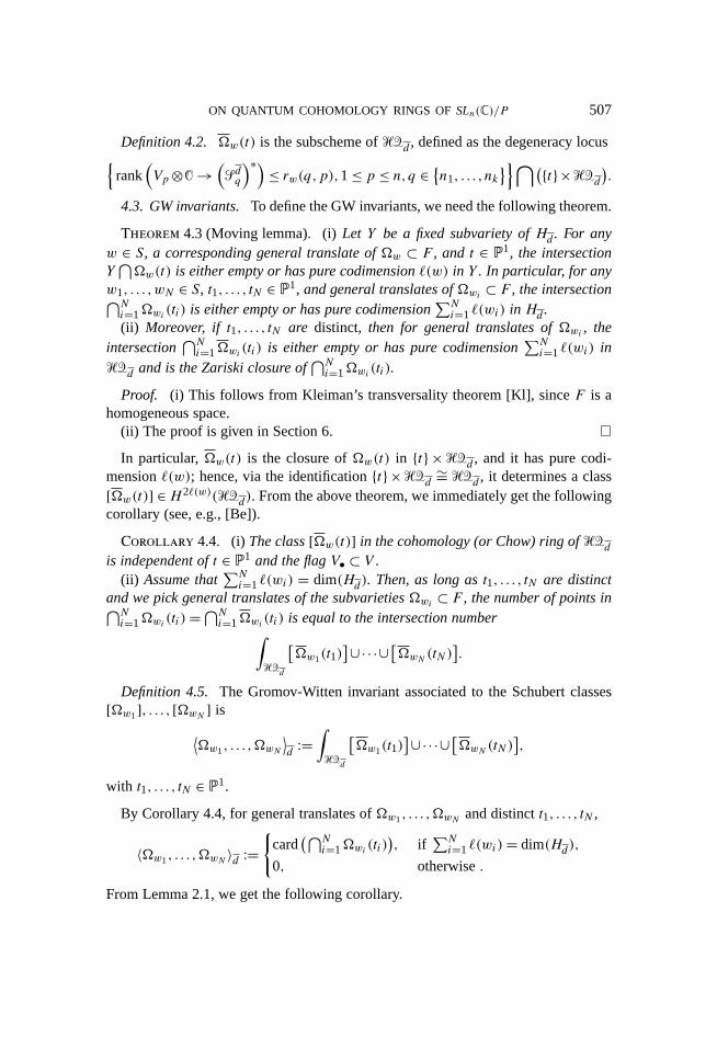
Definition 4.2. �w(t) is the subscheme of��d , defined as the degeneracy locus{rank
4.3. GW invariants.To define the GW invariants, we need the following theorem.
Theorem 4.3 (Moving lemma). (i) Let Y be a fixed subvariety ofHd . For anyw ∈ S, a corresponding general translate of�w ⊂ F , and t ∈ P1, the intersectionY⋂�w(t) is either empty or has pure codimension((w) in Y . In particular, for any
w1, . . . ,wN ∈ S, t1, . . . , tN ∈ P1, and general translates of�wi ⊂ F , the intersection⋂Ni=1�wi (ti) is either empty or has pure codimension
∑Ni=1((wi) in Hd .
(ii) Moreover, if t1, . . . , tN are distinct, then for general translates of�wi , theintersection
⋂Ni=1�wi (ti) is either empty or has pure codimension
∑Ni=1((wi) in
��d and is the Zariski closure of⋂Ni=1�wi (ti).
Proof. (i) This follows from Kleiman’s transversality theorem [Kl], sinceF is ahomogeneous space.
(ii) The proof is given in Section 6.
In particular,�w(t) is the closure of�w(t) in {t}��d , and it has pure codi-mension((w); hence, via the identification{t}��d
∼= ��d , it determines a class[�w(t)] ∈H 2((w)(��d). From the above theorem, we immediately get the followingcorollary (see, e.g., [Be]).
Corollary 4.4. (i) The class[�w(t)] in the cohomology (or Chow) ring of��dis independent oft ∈ P1 and the flagV• ⊂ V .
(ii) Assume that∑Ni=1((wi) = dim(Hd). Then, as long ast1, . . . , tN are distinct
and we pick general translates of the subvarieties�wi ⊂ F , the number of points in⋂Ni=1�wi (ti)=
⋂Ni=1�wi (ti) is equal to the intersection number∫
��d
[�w1(t1)
]∪·· ·∪[�wN (tN)].Definition 4.5. The Gromov-Witten invariant associated to the Schubert classes
[�w1], . . . , [�wN ] is⟨�w1, . . . ,�wN
⟩d:=∫
��d
[�w1(t1)
]∪·· ·∪[�wN (tN)],with t1, . . . , tN ∈ P1.
By Corollary 4.4, for general translates of�w1, . . . ,�wN and distinctt1, . . . , tN ,
〈�w1, . . . ,�wN 〉d :={
card(⋂N
i=1�wi (ti)), if
∑Ni=1((wi)= dim(Hd),
0, otherwise.
From Lemma 2.1, we get the following corollary.
508 IONUT CIOCAN-FONTANINE
Corollary 4.6. The invariant I3,d ([�w1][�w2][�w3]), defined using Kontse-
vich’s space of stable mapsM0,3(F,d), coincides with〈�w1,�w2,�w3〉d . Hence,
[�u]∗[�v]=∑
d
qd11 · · ·qdkk
∑w∈S
⟨�u,�v,�w
⟩d
[�w
].
When N > 3, 〈�w1, . . . ,�wN 〉d does not coincide with the GW invariantIn,d([�w1] · · · [�wN ]) of [KM], as they are solutions to different enumerative ge-ometry problems. However,〈�w1, . . . ,�wN 〉d can also be realized as an intersectionnumber on the Kontsevich moduli spaceM0,N (F,d), and, from this definition, it isnot hard to see that⟨
�w1, . . . ,�wN⟩d=
∑e+f=d
∑v∈S
⟨�w1, . . . ,�wN−2,�v
⟩e
⟨�v,�wN−1,�wN
⟩f,(4.1)
from which it follows that[�w1
]∗[�w2
]∗· · ·∗[�wN ]=∑d
qd11 · · ·qdkk
∑w∈S
⟨�w1, . . . ,�wN ,�w
⟩d
[�w
].(4.2)
We use (4.2) in Section 6 for the proof of Theorem 3.14.
Remark 4.7. (i) Sometimes (4.2) is used as the definition of the quantum multi-plication in the small quantum cohomology ring, and then (4.1) is equivalent to theassociativity of this multiplication.
(ii) (Compare [FoGP].) The relation (4.2), together with the quantum Giambelliformula and the orthogonality property of the quantum Giambelli polynomials, givesa direct (algebro-combinatorial) method to compute the GW invariants ofF . Namely,for anyw1, . . . ,wN ∈ S, we get∑
d
qd11 · · ·qdkk
⟨�w1, . . . ,�wN
⟩d= ⟨⟨Pqw1
× ·· · ×PqwN⟩⟩,(4.3)
where〈〈· · · 〉〉 is defined by(3.10). The Gröbner basis techniques for more efficientcomputations of the invariants, as described in [FoGP, Section 12] for the case ofcomplete flags, can be readily extended to cover the partial flag varieties as well.
We conclude this section by recording for later use a result similar to Theorem 4.3,due to Kim [Kim3, Corollary 3.2].
For every irreducible closed subvarietyY ⊂ F and everyt ∈ P1, we denote byY (t) the preimageev−1(Y )
⋂{t}×Hd and byY (t) the closure ofY (t) in {t}×��d .
Proposition 4.8. Let Y1, . . . ,YN be closed, irreducible subvarieties inF , and
ON QUANTUM COHOMOLOGY RINGS OFSLn(C)/P 509
let t1, . . . , tN be distinct points inP1. Assume that∑Ni=1codimYi = dimHd . Then
for general translates ofYi , the intersection scheme⋂Ni=1Yi(ti) is either empty or
consists of finitely many reduced points. Moreover,
N⋂i=1
Yi(ti)=N⋂i=1
Yi(ti),
and the cardinality of this set is equal to the intersection number∫��d
[Y1(t1)
]∪·· ·∪
[YN(tN)
].
Note that Theorem 4.3 does not follow from Proposition 4.8, since�w(t) may bea priori larger than the closure of�w(t).
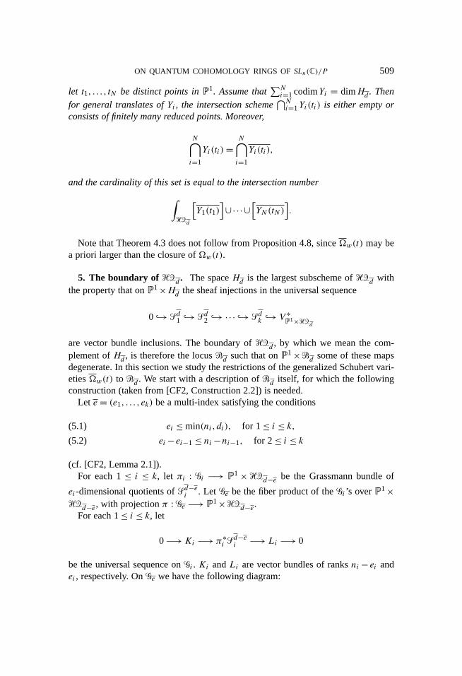
5. The boundary of��d . The spaceHd is the largest subscheme of��d withthe property that onP1×Hd the sheaf injections in the universal sequence
0 ↪→ �d1 ↪→ �d2 ↪→ ··· ↪→ �dk ↪→ V ∗P1×��d
are vector bundle inclusions. The boundary of��d , by which we mean the com-plement ofHd , is therefore the locus�d such that onP1�d some of these mapsdegenerate. In this section we study the restrictions of the generalized Schubert vari-eties�w(t) to �d . We start with a description of�d itself, for which the followingconstruction (taken from [CF2, Construction 2.2]) is needed.
Let e = (e1, . . . ,ek) be a multi-index satisfying the conditions
ei ≤ min(ni,di), for 1≤ i ≤ k,(5.1)
ei−ei−1 ≤ ni−ni−1, for 2≤ i ≤ k(5.2)
(cf. [CF2, Lemma 2.1]).For each 1≤ i ≤ k, let πi : �i −→ P1 × ��d−e be the Grassmann bundle of
ei-dimensional quotients of�d−ei . Let �e be the fiber product of the�i ’s overP1×��d−e, with projectionπ : �e −→ P1×��d−e.
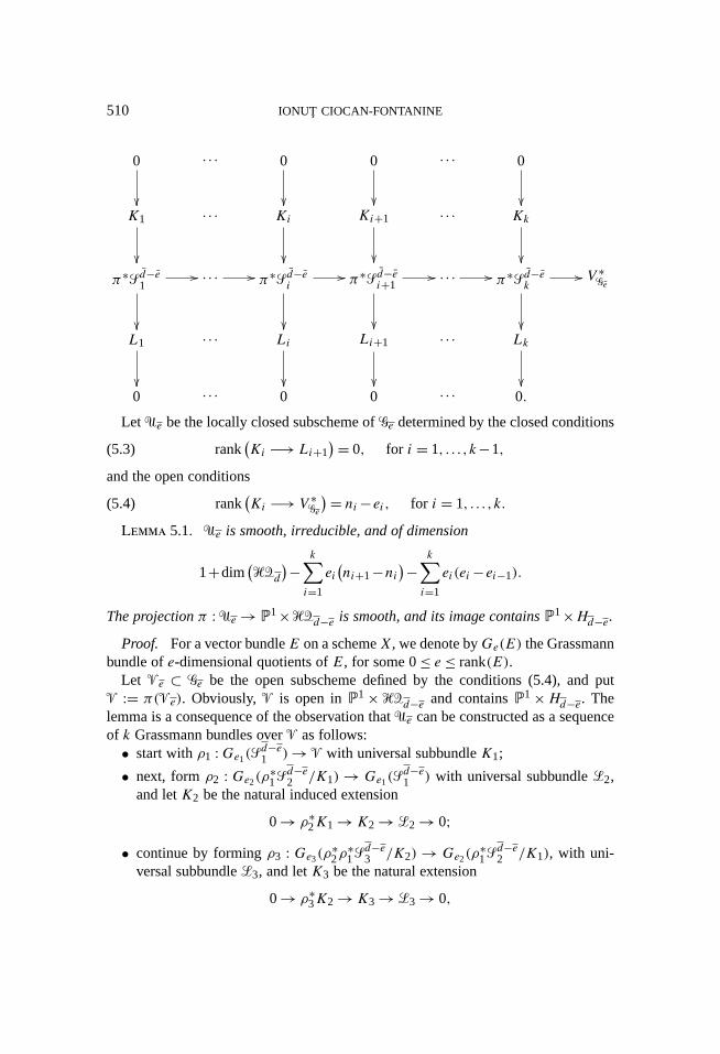
For each 1≤ i ≤ k, let
0−→Ki −→ π∗i �d−ei −→ Li −→ 0
be the universal sequence on�i . Ki andLi are vector bundles of ranksni− ei andei , respectively. On�e we have the following diagram:
510 IONUT CIOCAN-FONTANINE
0
��
· · · 0
��
0
��
· · · 0
��K1
��
· · · Ki
��
Ki+1
��
· · · Kk
��
π∗�d−e1
��
�� · · · �� π∗�d−ei��
��
π∗�d−ei+1
��
�� · · · �� π∗�d−ek
��
�� V ∗�e
L1
��
· · · Li
��
Li+1
��
· · · Lk
��0 · · · 0 0 · · · 0.
Let �e be the locally closed subscheme of�e determined by the closed conditions
rank(Ki −→ Li+1
)= 0, for i = 1, . . . ,k−1,(5.3)
and the open conditions
rank(Ki −→ V ∗
�e
)= ni−ei, for i = 1, . . . ,k.(5.4)
Lemma 5.1. �e is smooth, irreducible, and of dimension
1+dim(��d
)− k∑i=1
ei(ni+1−ni
)− k∑i=1
ei(ei−ei−1).
The projectionπ : �e → P1×��d−e is smooth, and its image containsP1×Hd−e.Proof. For a vector bundleE on a schemeX, we denote byGe(E) the Grassmann
bundle ofe-dimensional quotients ofE, for some 0≤ e ≤ rank(E).Let e ⊂ �e be the open subscheme defined by the conditions (5.4), and put
:= π(e). Obviously, is open inP1 × ��d−e and containsP1 ×Hd−e. Thelemma is a consequence of the observation that�e can be constructed as a sequenceof k Grassmann bundles over as follows:
• start withρ1 :Ge1(�d−e1 )→ with universal subbundleK1;
versal subbundle3, and letK3 be the natural extension
0→ ρ∗3K2 →K3 → 3 → 0,
ON QUANTUM COHOMOLOGY RINGS OFSLn(C)/P 511
and so on.We use this description of�e in the proof of quantum Pieri (see Section 6.3).
Theorem 5.2. There exist morphismsφe : �e −→ ��d with the following prop-erties.
(i) If rank(t,x)�dk−i+1 = n−ni+ei for every1≤ i ≤ k at a point(t,x) ∈ P1×��d ,thenx ∈ φe(�e). In particular,�d is covered by the union ofφe(�e), wheree rangesover all (nonzero) multi-indices satisfying (5.1) and (5.2).
(ii) The restriction ofφe to π−1(P1×Hd−e) is an isomorphism onto its image.
Proof. This proof is the same as the proof of [CF2, Theorem 2.3(ii)].
Lemma 5.3. We have
φ−1e
(�w(t)
)= π−1(P1×�w(t))⋃
�ew(t),
�ew(t) being the locus inside�e(t) := π−1({t}×��d−e), where
rank(Vp⊗� →K∗
q
)≤ rw(q,p),(5.5)
for all p = 1, . . . ,n, q ∈ {n1, . . . ,nk}.Proof. See [CF2, Lemma 3.1].
Following [CF2, Section 3], we now describe the locus�ew(t) of Lemma 5.3. Theanalysis there can be applied in our case without any changes; the only reason forreproducing part of it here is to fix the somewhat elaborate notation needed.
Let a := card{ni − ei | i = 1, . . . ,k}. Sete0 = ek+1 = 0 and define a partition of[0,k+1] as
i0 = 0, ij = min{i | ni−ei ≥ nij−1 −eij−1 +1}, for 1≤ j ≤ a, ia+1 = k+1.
Letmj = nij −eij , for j = 0,1, . . . ,a. By definition, on each of the intervals[1, i1−1
],[i1, i2−1
], . . . ,
[ia−1, ia−1
],[ia,k
],
ni−ei is constant and equal to 0,m1, . . . ,ma, respectively. The corresponding bundlesK∗i are all isomorphic. Therefore, we can restrict the set of rank conditions (5.5),
defining�ew(t) inside�e(t), to
rank(Vp⊗� →K∗
q
)≤ rw(q,p), for 1≤ p ≤ n,q ∈ {ni1, . . . ,nia}.(5.6)
Moreover, we can further modify (5.6). Define recursivelyr := (rj,p)1≤p≤n,1≤j≤aas follows:
r1,p = min{rw(ni1,p),m1
}, 1≤ p ≤ n,
rj,p = min{rw(nij ,p
), rj−1,p+mj −mj−1
}, for 1≤ p ≤ n,2≤ j ≤ a.
512 IONUT CIOCAN-FONTANINE
Lemma 5.4. The conditions
rank(Vp⊗� →K∗
ij
)≤ rj,p, for 1≤ p ≤ n,1≤ j ≤ a(5.7)
define the same degeneracy locus�ew(t) in �e(t).
Proof. See [CF2, Construction 3.5].
Lemma 5.5. (i) There exists a unique permutationwe ∈ Sn such that ifwe(q) >we(q + 1), thenq ∈ {m1, . . . ,ma} and rj,p = rwe (mj ,p), for all 1 ≤ p ≤ n,1 ≤j ≤ a.
(ii) We have((w)−((we)≤∑ki=1ei(ni+1−ni).
Proof. The following explicit construction ofwe is taken from [CF2, Lemma 3.6].For eachj = 0,1, . . . ,a+1, define setsWj(w) by
W0(w)= ∅, Wj (w)={w(1), . . . ,w
(nij)}.
Also, we define setsZj(w) andorderedsetsZj (w) such that(a) cardZj(w)= nij −mj−1,
(b) cardZj (w)=mj −mj−1,(c) Zj (w)
⋂Zj ′(w)= ∅, if j �= j ′,
(d)⋃a+1j=1 Zj (w)= [1,n], by the following recursive procedure.
Let Z0(w)= Z0(w)= ∅. If Zi(w) was already defined fori = 0,1, . . . , j−1, let
Now definewe(q)= zq , for all 1≤ q ≤ n.The estimate (ii) follows (cf. [CF2, Lemma 3.8]) by first noticing that the difference
((w)− ((we) is maximized by the longest permutationw◦, defined byw◦(i) =n−nj + i−nj−1, for all nj−1+1 ≤ i ≤ nj and 1≤ j ≤ k+1. For this case, onecomputes directly that we have, in fact, the equality
((w◦)−(((w◦)e)= k∑
i=1
ei(ni+1−ni).
ON QUANTUM COHOMOLOGY RINGS OFSLn(C)/P 513
Remark 5.6. (i) In the terminology of [F1], Lemma 5.5(i) says thatr is apermis-siblecollection of rank numbers.
(ii) Let Fe := F(m1, . . . ,ma,V ) be the partial flag variety corresponding to themi ’s. The sequence of quotient bundles
V ⊗��e(t) �K∗nia
� · · · �K∗ni1
is the pullback via a uniquely determined morphismψe(t) : �e(t) → Fe of thetautological sequence of quotient bundles onFe. By Lemmas 5.4 and 5.5(i),we
defines a Schubert variety onFe, and we have�ew(t)= ψe(t)−1(�we ).
Finally, we spell out in more detail what the analysis in this section says for somespecial cases.
Lemma 5.7. Let (e1, . . . ,ek) be a multi-index. Fix1≤ j ≤ k and1≤ i ≤ nj , andconsider the cycleαi,j := snj−i+1× ·· · ×snj . Then
αei,j =
αi,j , if ej = 0,
αi,j ·snj × ·· · ×snj−ej+1, if 1≤ ej < i,id, if i ≤ ej .
In particular, ((αi,j )−((αei,j )≤ ej , with equality if and only ifej ≤ i.Proof. The proof is immediate from the construction ofαei,j in Lemma 5.5.
Lemma 5.8 (Compare [CF2, Lemma 3.9]). Assume in addition thate �= (0, . . . ,0).Then we have the following.
(i)∑ki=1ei(ei−ei−1)≥ ej , for 1≤ j ≤ k. In particular,
∑ki=1ei(ei−ei−1)≥ 1.
(ii) There exists1 ≤ j ≤ k such that∑ki=1ei(ei − ei−1) = ej if and only if there
are integers1≤ h1< h2< · · ·< hm ≤ j ≤ lm < · · ·< l2< l1 ≤ k such that
ei =
0, for i ∈ [1,h1−1]∪[l1+1,k],1, for i ∈ [h1,h2−1]∪[l2+1, l1],2, for i ∈ [h2,h3−1]∪[l3+1, l2],· · ·m, for i ∈ [hm, lm]
(in particular, ej =m).(iii) Let ehl denote a multi-index as in (ii), and letw ∈ S be any permutation. Let
wehl be the permutation given by Lemma 5.5(i). Then
((w)−((wehl )= k∑i=1
ei(ni+1−ni
)= m∑c=1
(nlc+1−nhc
)
514 IONUT CIOCAN-FONTANINE
if and only if for every1≤ i ≤m we have
w(nhi)>max
{w(nhi +1
), . . . ,w
(nli),w(nli+1
)}.
In this case,wehl = w ·γhm,lm ·γhm−1,lm−1 × ·· · ×γh1,l1, whereγh,l denotes the cyclicpermutationsnh× ·· · ×snl+1−1 (cf. the paragraph before Theorem 3.1).
Proof. (i) First, using the easy identity
k∑i=1
ei(ei−ei−1)= 1
2
[e21+(e2−e1)2+·· ·+(ek−ek−1)
2+e2k]
and the change of variablesx1 = e1,x2 = e2−e1, . . . ,xk = ek−ek−1,xk+1 = ek, theinequality in (i) becomes
j∑i=1
(x2i −2xi
)+ k+1∑i=j+1
x2i ≥ 0,(5.8)
with the additional constraintxk+1 =∑ki=1xi . Now (5.8) is equivalent to
j∑i=1
(xi−1)2+k+1∑i=j+1
x2i ≥ j.(5.9)
Changing variables again toy1 = x1−1, . . . ,yj = xj −1,yj+1 = xj+1, . . . ,yk+1 =xk+1, we are reduced to proving
k+1∑i=1
y2i ≥ j,(5.10)
subject to the constraint
yk+1 = j+k∑i=1
yi.(5.11)
Replacingj in (5.10) byyk+1−∑ki=1yi , we need to show that
(y2k+1−yk+1
)+ k∑i=1
(y2i +yi
)≥ 0.(5.12)
Sinceyi , for 1≤ i ≤ k+1, are integers, bothy2k+1−yk+1 andy2
i +yi are nonnegativeand (5.12) follows.
(ii) We have equality in (5.12) if and only ifyk+1 is equal to either zero or 1, andeachyi , for 1≤ i ≤ k, is equal to either zero or−1. Using (5.11), we see that equalityoccurs in one of the following two cases:
ON QUANTUM COHOMOLOGY RINGS OFSLn(C)/P 515
• eitheryk+1 = 0, exactlyj amongy1, . . . ,yk are equal to−1, and the rest areequal to zero;
• or yk+1 = 1, exactlyj −1 amongy1, . . . ,yk are equal to−1, and the rest areequal to zero.
Changing the variables back toei , the statement in (ii) is obtained.(iii) This follows by the construction ofwehl .
6. Proofs of themoving lemma, the quantumPieri formula, and Theorem 3.14.This section is devoted to the proofs of Theorem 4.3(ii), Theorem 3.1, and Theo-rem 3.14. For this purpose we heavily use the structure of the boundary of��d ,described in the preceding section.
Throughout the rest of the paper, we work with suitable general translates of theSchubert varieties (or any other subvarieties) inF .
6.1. Proof of Theorem 4.3(ii) (Compare [CF2, Theorem 4.1]).We proceed byinduction ond. If d1 = ·· · = dk = 0, then��d = Hd = F , and there is nothing toprove. Assume that the statement is true for allf such thatfi ≤ di , for 1≤ i ≤ k, andfj < dj , for some 1≤ j ≤ k. Let c :=∑N
i=1((wi). By Theorem 4.3(i) and Theorem5.2(i), it is enough to show that
codim��d
(N⋂i=1
�wi (ti)
)⋂φe(�e) > c,(6.1)
for every multi-indexe �= (0, . . . ,0), satisfying conditions (5.1) and (5.2). UsingTheorem 5.2(ii) and Lemma 5.1, the inequality (6.1) follows if we prove that thecodimension of
⋂Ni=1φ
−1e (�wi (ti)) in �e is greater than
c−(dim��d−dim�e)= c+1−k∑i=1
ei(ni+1−ni)−k∑i=1
ei(ei−ei−1).
By Lemma 5.3, we have to prove the same estimate for the codimension of
N⋂i=1
(π−1(P1×�wi (ti)
)⋃�ewi (ti)
)(6.2)
in �e. Since the pointst1, . . . , tN are distinct, the only possibly nonempty intersectionsin (6.2) contain either no�ewi (ti) term or only one such term. If there is no such term,the required inequality follows from the induction assumption on��d−e and the factthatπ is a smooth map. After possibly renumbering the pointsti , to finish the proofit suffices to show the estimate for
W⋂�ewN (tN )⊂ �e(tN ),(6.3)
516 IONUT CIOCAN-FONTANINE
where
W :=N−1⋂i=1
(π−1({tN }×�wi (ti)))
and�e(tN )= π−1({tN }×��d−e). By the induction assumption,W has codimensionc−((wN) in �e(tN ), while by Remark 5.6(ii) and Kleiman’s theorem on transversalityof general translates, the intersection (6.3) has codimension((weN) inW . The estimatefollows now from Lemma 5.5(ii) and Lemma 5.8(i).
6.2. Computing GW invariants via degenerations.For the proofs of quantum Pieriand of Theorem 3.14, we need to compute certain invariants〈�w1, . . . ,�wN 〉d . Thetechnique we use is to degenerate the intersection
⋂Ni=1�wi (ti) by allowing some of
the pointsti to coincide. This procedure may lead to contributions supported on theboundary, which can be evaluated using the analysis in Section 5. In this subsection,we summarize some results of this type.
The following is an easy consequence of Proposition 4.8 and Theorem 4.3. For aproof, see, for instance, [Be, Lemma 2.5].
Lemma 6.1. Let Y1, Y2 be subvarieties inF such thatcodimY1 + codimY2 =dim��d , and lett1, t2 ∈ P1 be distinct points. Assumed �= (0, . . . ,0). Then∫
��d
[Y1(t1)
]∪[Y2(t2)
]= 0.
In particular, for anyv,w ∈ S,⟨�v,�w
⟩d={
1, if d = (0, . . . ,0) andv = w,0, otherwise.
Lemma 6.2. Let d be a multi-index, and letv1, . . . ,vN ,w1, . . . ,wM ∈ S satisfy∑Ni=1((vi)+
that the conclusion of Theorem 4.3(ii) holds for the intersection
�v1(y)⋂
· · ·⋂�vN (y)
⋂�w1(t1)
⋂· · ·⋂�wM(tM).(6.4)
LetY :=�v1⋂ · · ·⋂�vN ⊂ F . Then
⟨�v1, . . . ,�vN ,�w1, . . . ,�wM
⟩d=∫
��d
[Y (y)
]∪[�w1(t1)]∪·· ·∪
[�wN (tN)
].
Proof. By Theorem 4.3(i), the intersection
�v1(y)⋂
· · ·⋂�vN (y)
⋂�w1(t1)
⋂· · ·⋂�wM(tM)⊂Hd
ON QUANTUM COHOMOLOGY RINGS OFSLn(C)/P 517
has pure dimension zero, and by assumption it coincides with (6.4). On the otherhand, we have
�v1(y)⋂
· · ·⋂�vN (y)= ev−1(Y )
⋂{y}×Hd.
The lemma follows now from the definition of〈· · · 〉d , Corollary 4.4, and Proposition4.8.
Proposition 6.3. Letd �= (0, . . . ,0) be a multi-index; letu,v,w ∈ S be such that((u)+((v)+((w)= dimHd ; and lety, t ∈ P1 be distinct points. Denote
Z :=�u(y)⋂�v(y)
⋂�w(t)⊂ ��d .
Assume thatZ is either empty or purely zero-dimensional. Then(i) Z is contained in�d ;(ii) [Z] = [�u(y)]∪[�v(y)]∪[�w(t)] is a cycle of degree〈�u,�v,�w〉d .Proof. (i) Write �u
⋂�v = Y insideF . Let Z′ be the (largest) subscheme ofZ
supported onHd . Then, as in the proof of Lemma 6.2, we have
Z′ = Y (y)⋂�w(t);
hence, by Proposition 4.8,
cardZ′ =∫
��d
[Y (y)
]∪[�w(t)
].
By Lemma 6.1,Z′ is empty.(ii) Let V := �v(y)⋂�w(t) ⊂ ��d , and consider the trivial familyP1×V ⊂
P1×��d overP1. Let ρ : X ↪→ P1×��dpr−→ P1 be the family whose fibre over
x ∈ P1 is the generalized Schubert variety�u(x). It follows from Theorem 4.3 thatρis a fibre bundle map (see, e.g., [Be, Corollary 2.4]), and in particular it is flat. Sincethe intersection(P1×V )⋂X is obviously proper overP1, the proposition followsfrom [F2, Example 10.2.1].
6.3. Proof of quantum Pieri.We formulate first an auxiliary lemma, for which weintroduce some notation.
Let X be a scheme. LetV be ann-dimensional complex vector space, and letBi , for 1≤ i ≤ k, be vector bundles onX, of ranksbi , respectively. Fix an integerj ∈ {1,2, . . . ,k}. Assume that we are given a sequence of generically injective maps
B1 → ··· → Bj−1 → Bj → Bj+1 → ··· → Bk → V ∗⊗�X.
Moreover, assume thatBi → V ∗ is an injective map of bundles for 1≤ i ≤ j . Fix0 ≤ e ≤ bj − bj−1, and letρ : Ge(Bj/Bj−1) → X be the Grassmann bundle ofe-dimensional quotients ofBj/Bj−1, with universal sequence
0→ L→ ρ∗(Bj/Bj−1)→Q→ 0.
518 IONUT CIOCAN-FONTANINE
LetK be the natural induced extension
0→ ρ∗Bj−1 →K→ L→ 0;that is,K is the kernel ofρ∗Bj →Q.
Let V1 ⊂ ·· · ⊂ Vn−1 ⊂ V be a fixed flag, and letw ∈ Sn be a permutation suchthat if w(q) > w(q+1), thenq ∈ {b1, . . . ,bj−1,bj −e,bj+1, . . . ,bk}. Denote byDwthe degeneracy locus onGe(Bj/Bj−1) determined by
Define a permutationw ∈ Sn as follows:• let {z1< z2< · · ·< zbj−bj−1} be the set{w(bj−1+1),w(bj−1+2), . . . ,w(bj )},
ordered increasingly;• if q /∈ {bj−1+1,bj−1+2, . . . ,bj }, setw(q)= w(q);• for 1≤ i ≤ bj −bj−1, setw(bj−1+ i)= zi .Lemma 6.4. (i) The imageρ(Dw) is the degeneracy locusDw onX defined by
rank(Vp⊗� → B∗
q
)≤ rw(q,p), 1≤ p ≤ n,q ∈ {b1, . . . ,bk}.(6.7)
(ii) The restriction ofρ to Dw has positive dimensional fibres, unless
If (6.8) holds andDw is irreducible, thenρ mapsDw birationally ontoDw.
Proof. First note that if (6.8) is satisfied, then (6.9) follows directly from thedefinition ofw.
By the construction ofw, we haverw(bj ,p)= rw(bj ,p), for all 1≤ p ≤ n. Sincew(bj ) < w(bj + 1) by assumption, it follows from [F1, Proposition 4.2] that byadding the conditions
rank(Vp⊗� → (ρ∗Bj )∗
)≤ rw(bj ,p), for 1≤ p ≤ n,to (6.5) and (6.6), we obtain thesamelocusDw onGe(Bj/Bj−1). In other words,Dwis contained inρ−1(Dw). Consider the Grassmann bundle obtained by restriction:
ρ : ρ−1(Dw)→ Dw.
ON QUANTUM COHOMOLOGY RINGS OFSLn(C)/P 519
It is not hard to see thatDw is a Schubert variety in this bundle, of positive relativedimension, unless (6.8) holds, in which case it intersects each fibre in a point. Thelemma follows.
We now prove the following equivalent reformulation of Theorem 3.1.
Theorem 3.1′. The GW number〈�αi,j ,�w,�v〉d vanishes, unlessd is one of themulti-indicesehl of Lemma 5.8, such that((w ·γhl)= ((w)−∑m
c=1(nlc+1−nhc) andv is dual to one of the permutationsw′′ ·δhl , in which case it is equal to1.
Proof of Theorem3.1′. The idea is to degenerate the corresponding intersectionof generalized Schubert varieties, as in the previous subsection. Specifically, letd beany multi-index not identically zero, and letv ∈ S be such thatc := i+((w)+((v)=dimHd . Let y, t ∈ P1 be distinct points.
Claim 6.5. The intersection
Z :=�αi,j (y)⋂�w(y)
⋂�v(t)(6.10)
is either empty or purely zero-dimensional.
Proof. Indeed, by Theorem 4.3(i), it is enough to show that the restriction ofZ to�d is either empty or purely of dimension zero. As in the proof of Theorem 4.3(ii),this reduces to showing that the codimension in�e of(
φ−1e
(�αi,j (y)
))⋂(φ−1e
(�w(y)
))⋂(φ−1e
(�v(t)
))(6.11)
is at leastc+1−∑ki=1ei(ni+1−ni)−∑k
i=1ei(ei−ei−1), for all multi-indicese �=(0, . . . ,0), satisfying (5.1) and (5.2). By Lemma 5.3, the terms in (6.11) can berewritten as
π−1(P1×�αi,j (y))⋃
�eαi,j (y),
π−1(P1×�w(y))⋃
�ew(y),
π−1(P1×�v(t))⋃
�ev(t),
respectively. We have seen already in the proof of Theorem 4.3(ii) that the onlypossibly nonempty intersection is
�eαi,j (y)⋂�ew(y)
⋂π−1({y}×�v(t)),
which lies inside�e(y). But we can rewrite this as
ψe(y)−1(�αei,j
)⋂ψe(y)
−1(�we)⋂π−1({y}×�v(t)),(6.12)
520 IONUT CIOCAN-FONTANINE
whereψe(y) : �e(y)→ Fe is the morphism of Remark 5.6(ii). The codimension of(6.12) in�e(y) is
((αei,j
)+((we)+((v)by Kleiman’s transversality theorem; hence, its codimension in�e is
1+((αei,j )+((we)+((v)= 1+c−(((αi,j )−((αei,j ))−(((w)−((we)).The required estimate follows now from Lemmas 5.5(ii), 5.7, and 5.8(i).
By Claim 6.5 and Proposition 6.3, the GW invariant〈�αi,j ,�w,�v〉d can be com-puted as the degree of[Z] in the Chow ring of the hyperquot scheme. But we knoweven more! Namely, ifZ is nonempty, all the inequalities we used for the codimensionestimates in the proof of Claim 6.5 must in fact be equalities. By Lemma 5.8(ii) and(iii), this implies thatZ is contained in the (disjoint!) union of “strata”⋃
ehl
φehl(�ehl (y)
),
where the union is over allehl , such that((w · γhl) = ((w)−∑mc=1(nlc+1 − nhc).
Moreover, for eachehl , as above, the preimageφ−1ehl(Z) is given by the intersection
(6.12), withe replaced byehl .At this point we need the following lemma.
Granting this for a moment, we complete the proof of quantum Pieri. Recall that�ehl (y) can be realized as a succession of Grassmann bundles over an open subscheme ⊂ {y}×��d−ehl (cf. the proof of Lemma 5.1). Lemma 6.6 says thatZ is empty,
except possibly whend is one of the multi-indicesehl described above. In this case,
{y}×��d−ehl = = {y}×Hd−ehl = {y}×F,and�ehl (y) is projective. Moreover, the mapφehl (y) : �ehl (y)→ ��d is an embed-ding, by Theorem 5.2(ii). It follows that the degree of[Z] in the Chow ring of��dis given by ∫
�ehl (y)ψ ehl (y)
∗[�αehli,j
]∪ψehl (y)∗
[�wehl
]∪π∗[�v].(6.13)
Applying the classical Pieri formula (Theorem 1.5) onFehl , we can rewrite (6.13) as∑wehl
αehli,j−−→w′′
∫�ehl (y)
ψ ehl (y)∗[�w′′
]∪π∗[�v].
ON QUANTUM COHOMOLOGY RINGS OFSLn(C)/P 521
The subschemeψehl (y)−1(�w′′) is the degeneracy locus inside�ehl (y) determined
By Kleiman’s transversality theorem, we may assume that bothψehl (y)−1(�w′′)
and the intersectionψehl (y)−1(�w′′)
⋂π−1(�v) have the expected codimension.
Hence,ψehl (y)
∗[�w′′]∪π∗[�v]= [
ψehl (y)−1(�w′′
)⋂π−1(�v)]
in the Chow ring of�ehl (y). Recall thatπ : �ehl (y) → F can be realized as asuccession of Grassmann bundle projections (cf. the proof of Lemma 5.1). ApplyingLemma 6.4(i) to each of these Grassmann bundles, starting from the top, we get thatthe image ofψehl (y)
−1(�w′′) under the projectionπ is the Schubert variety�w′′′ ⊂ F ,wherew′′′ is the permutation (inS !) obtained fromw′′ by the successive applicationsof Lemma 6.4(i). By Lemma 6.4(ii), it follows thatπ ∗[ψehl (y)−1(�w′′)] = 0, unlessthe condition (6.8) is satisfied in every instance where we have used Lemma 6.4(i),in which caseπ∗[ψehl (y)−1(�w′′)] = [�w′′′ ].
Moreover, if this happens, the permutationw′′′ is obtained fromw′′ by applyingsuccessively the recipe (6.9). Using the fact that the simple transpositionssi andsj commute wheneveri and j are not consecutive integers, it follows easily thatw′′′ = w′′ ·δhl and
((w′′′)= ((w′′ ·δhl
)= ((w′′)−m−m∑c=1
(nlc−nhc−1
).
From the projection formula,∫F
π∗[ψehl (y)
−1(�w′′)⋂
π−1(�v)]= ∫F
[�w′′·δhl
]∪[�v].(6.15)
By Theorem 1.2, the latter intersection number vanishes, unlessv is the permutationin S dual tow′′ ·δhl , in which case it is equal to 1. This implies that the same holdsfor the intersection number (6.13).
Summarizing, deg[Z] vanishes, unless all the conditions stated in Theorem 3.1′ aresatisfied, in which case it is equal to 1, and moreover, we have seen that deg[Z] =〈�αi,j ,�w,�v〉d . This completes the proof of quantum Pieri.
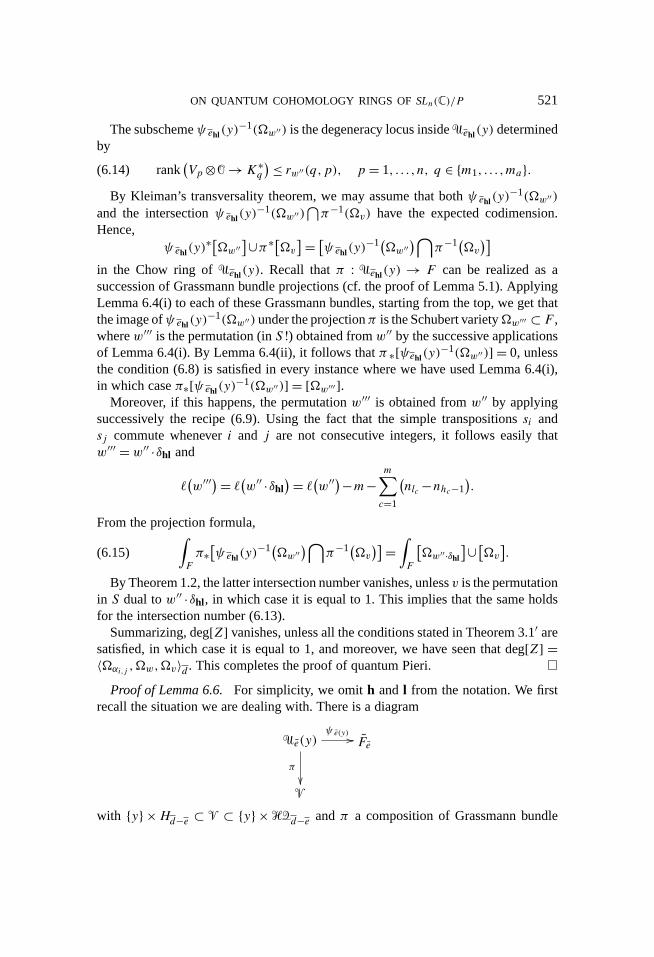
Proof of Lemma 6.6.For simplicity, we omith and l from the notation. We firstrecall the situation we are dealing with. There is a diagram
�e(y)ψ e(y) ��
π
��
Fe
with {y} ×Hd−e ⊂ ⊂ {y} ×��d−e andπ a composition of Grassmann bundle
522 IONUT CIOCAN-FONTANINE
projections. Let
W := �eαi,j (y)⋂�ew(y)= ψe(y)−1
(�αei,j
)⋂ψe(y)
−1(�we).We may assume thatW is irreducible, of the expected codimension((αei,j )+((we),while the intersectionW
⋂π−1({y}×�v(t)) is a nonempty finite set consisting of
reduced points and supported onπ−1({y}×Hd−e). It then follows thatπ(W)⋂({y}×
�v(t)) is a nonempty zero-dimensional subscheme of{y}×Hd−e. By Lemma 6.1,this would imply d = e and therefore conclude the proof, if we can show thatπ(W)
⋂({y}×Hd−e) is of the formY (y), for someY ⊂ F . SetY := evy(π(W)),
whereevy is the restriction of the evaluation map to{y}×Hd−e. Thenπ(W)⊂ Y (y).To get the reverse inclusion, it suffices to show that if there exists a mapf : P1 → F
with [f ] ∈ π(W), then for everyg : P1 → F such thatg(y) = f (y) we have[g] ∈ π(W) as well. The mapf is represented by a sequence of subbundles
S1 ⊂ S2 ⊂ ·· · ⊂ Sk ⊂ V ∗⊗�P1.
By assumption, there exists a point inW ⊂ �e(y), lying over[f ]. This is equivalentto saying that for everyi ∈ {1, . . . ,k} there exist quotients
Si(y)� Cei(6.16)
of the fibres aty, together with compatible mapsCei → Cei+1, and which satisfythe degeneracy conditions defining�eαi,j (y) and �ew(y). If g is another map andg(y)= f (y), then the flag of fibres aty for the sequence of subbundles correspondingto g coincides with
S1(y)⊂ S2(y)⊂ ·· · ⊂ Sk(y)⊂ V ∗⊗�y.
Hence, we can take thesamequotients(6.16) to obtain a point inW lying over [g].The lemma is proved.
6.4. Proof of Theorem 3.14.By the relation (4.2), it suffices to show that〈�w1, . . . ,�wN ,�v〉d = 0, for everyv ∈ S and for everyd not identically zero.We may assume that((v)+∑N
j=1((wj ) = dimHd . Let y, t ∈ P1 be distinct points,and let
�w1
⋂· · ·⋂�wN := Y ⊂ F.
By Lemma 5.7 and conditions(1) and(2) in Theorem 3.14, for every multi-indexewe have the inequality
N∑m=1
(((wm)−(
(wem
))≤ k∑j=1
ej(nj+1−nj
).
ON QUANTUM COHOMOLOGY RINGS OFSLn(C)/P 523
Using this, codimension estimates similar to the ones in the proofs of Theorem 4.3(ii)and Claim 6.5 show that the intersection
�w1(y)⋂
· · ·⋂�wN (y)
⋂�v(t)
misses the boundary of��d . Therefore we can apply Lemma 6.2 to conclude that⟨�w1, . . . ,�wM ,�v
⟩d=∫
��d
[Y (y)
]∪[�v(t)
].
By Lemma 6.1, all such intersection numbers vanish wheneverd �= (0, . . . ,0).References
[AS] A. Astashkevich and V. Sadov, Quantum cohomology of partial flag manifoldsFn1,...,nk ,Comm. Math. Phys.170 (1995), 503–528.
[Beh] K. Behrend, Gromov-Witten invariants in algebraic geometry, Invent. Math.127 (1997),601–617.
[BehM] K. Behrend and Y. Manin, Stacks of stable maps and Gromov-Witten invariants, DukeMath. J.85 (1996), 1–60.
[BGG] I. N. Bernstein, I. M. Gelfand, and S. I. Gelfand, Schubert cells and cohomology of thespacesG/P , Russian Math. Surveys28 (1973), 1–26.
[Be] A. Bertram, Quantum Schubert calculus, Adv. Math.128 (1997), 289–305.[Bor] A. Borel, Sur la cohomologie des espaces fibrés principaux et des espaces homogènes de
groupes de Lie compacts, Ann. of Math. (2)57 (1953), 115–207.[CF1] I. Ciocan-Fontanine, Quantum cohomology of flag varieties, Internat. Math. Res. Notices
1995, 263–277.[CF2] , The quantum cohomology ring of flag varieties, to appear in Trans. Amer. Math.
Soc.[CFF] I. Ciocan-Fontanine and W. Fulton, “Quantum double Schubert polynomials” inSchu-
bert Varieties and Degeneracy Loci, Lecture Notes in Math.1689, Springer-Verlag,New York, 1998, 134–137.
[D] M. Demazure, Désingularisation des variétés de Schubert généralisées, Ann. Sci. ÉcoleNorm. Sup. (4)7 (1974), 53–88.
[E] C. Ehresmann, Sur la topologie de certains espaces homogènes, Ann. of Math. (2)35(1934), 396–443.
[FoGP] S. Fomin, S. Gelfand, and A. Postnikov, Quantum Schubert polynomials, J. Amer. Math.Soc.10 (1997), 565–596.
[F1] W. Fulton, Flags, Schubert polynomials, degeneracy loci, and determinantal formulas,Duke Math. J.65 (1992), 381–420.
[F2] , Intersection Theory, 2d ed., Springer-Verlag, Berlin, 1998.[F3] , Universal Schubert polynomials, Duke Math. J.96 (1999), 575–594.[FP] W. Fulton and R. Pandharipande, “Notes on stable maps and quantum cohomology” in
Algebraic Geometry (Santa Cruz, Calif., 1995), Proc. Sympos. Pure Math.62, Part2, Amer. Math. Soc., Providence, 1997, 45–96.
[GK] A.Givental andB. Kim, Quantum cohomology of flag manifolds and Toda lattices, Comm.Math. Phys.168 (1995), 609–641.
[Kim1] B. Kim, Quantum cohomology of partial flag manifolds and a residue formula for theirintersection pairings, Internat. Math. Res. Notices1995, 1–15.
[Kim3] , Gromov-Witten invariants for flag manifolds, thesis, University of California,Berkeley, 1996.
[KiMa] A. N. Kirillov and T. Maeno, Quantum double Schubert polynomials, quantum Schubertpolynomials and Vafa-Intriligator formula, to appear in Discrete Math.
[Kl] S. Kleiman, The transversality of a general translate, Compositio Math.28 (1974), 287–297.
[K] M. Kontsevich, “Enumeration of rational curves via torus actions” inThe Moduli Spaceof Curves (Texel Island, Netherlands, 1994), Progr. Math.129, Birkhauser, Boston,1995, 335–368.
[KM] M. Kontsevich and Y. Manin, Gromov-Witten classes, quantum cohomology and enumer-ative geometry, Comm. Math. Phys.164 (1994), 525–562.
[LS] A. Lascoux and M.-P. Schützenberger, Polynômes de Schubert, C. R. Acad. Sci. ParisSér. I Math.294 (1982), 447–450.
[Lau] G. Laumon, Un analogue global du cône nilpotent, Duke Math. J.57 (1988), 647–671.[LiT1] J. Li and G. Tian, The quantum cohomology of homogeneous varieties, J. Algebraic Geom.
6 (1997), 269–305.[LiT2] , Virtual moduli cycles and Gromov-Witten invariants of algebraic varieties, J. Amer.
Math. Soc.11 (1998), 119–174.[M] I. G. Macdonald, Notes on Schubert Polynomials, LaCIM, Département de Mathématiques
et d’Informatique, Université du Québec à Montréal, 1991.[McS] D. McDuff and D. Salamon, J-holomorphic curves and quantum cohomology, Univ. Lec-
ture Ser.6, Amer. Math. Soc., Providence, 1994.[Pe] D. Petersen, lecture, University of Washington, May 1996.[Po] A. Postnikov, On a quantum version of Pieri’s formula, to appear inProgress in Geometry,
Birkhäuser, Boston.[RT] Y. Ruan andG. Tian, A mathematical theory of quantum cohomology, J. Differential Geom.
42 (1995), 259–367.[ST] B. Siebert and G. Tian, On quantum cohomology rings of Fano manifolds and a formula
of Vafa and Intriligator, Asian J. Math.1 (1997), 679–695.[So] F. Sottile, Pieri’s formula for flag manifolds and Schubert polynomials, Ann. Inst. Fourier
(Grenoble)46 (1996), 89–110.[T] G. Tian, “Quantum cohomology and its associativity” inCurrent Developments in Math-
ematics (Cambridge, Mass., 1995), International Press, Cambridge, Mass., [1994],361–401.
[Va] C. Vafa, “Topological mirrors and quantum rings” inEssays on Mirror Manifolds, ed. S. T.Yau, International Press, Hong Kong, 1992, 96–119.
[Ve] S. Veigneau, Calcul symbolique et calcul distribué en combinatoire algébrique, thesis,Université Marne-la-Vallée, 1996.
[W1] E. Witten, “Two-dimensional gravity and intersection theory on moduli space” inSurveysin Differential Geometry (Cambridge, Mass., 1990), Lehigh Univ., Bethlehem, Pa.,1991, 243–310.
[W2] , “The Verlinde algebra and the cohomology of the Grassmannian” inGeometry,Topology, and Physics, Conf. Proc. Lecture Notes Geom. Topology4, InternationalPress, Cambridge, Mass., 1995, 357–422.
Department of Mathematics, Northwestern University, 2033Sheridan Road, Evanston,Illinois 60208-2730, USA; [email protected]