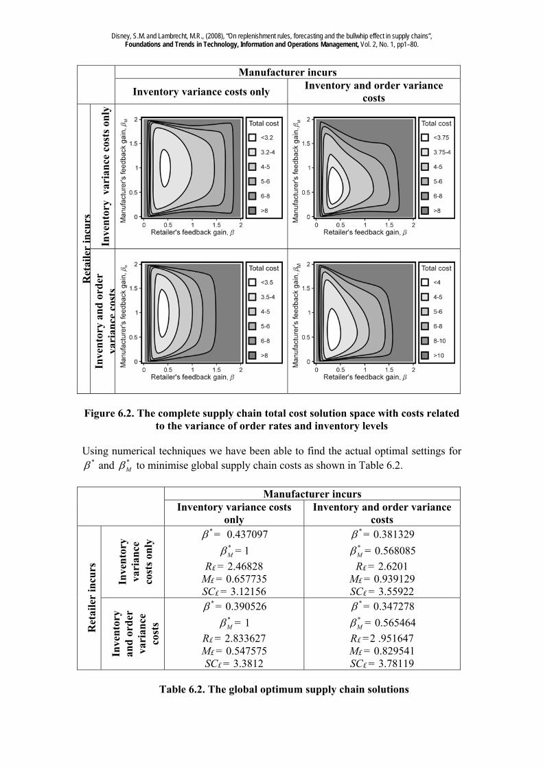
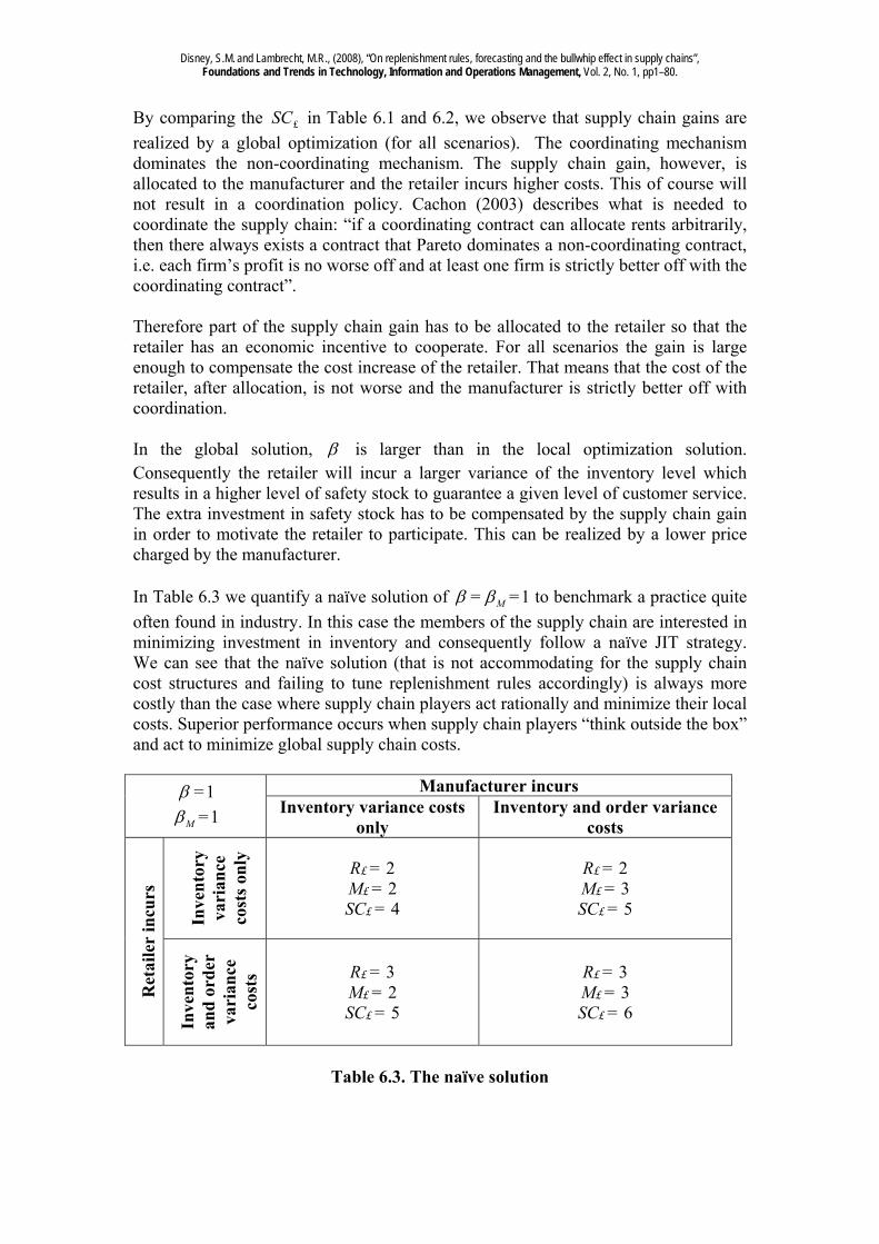
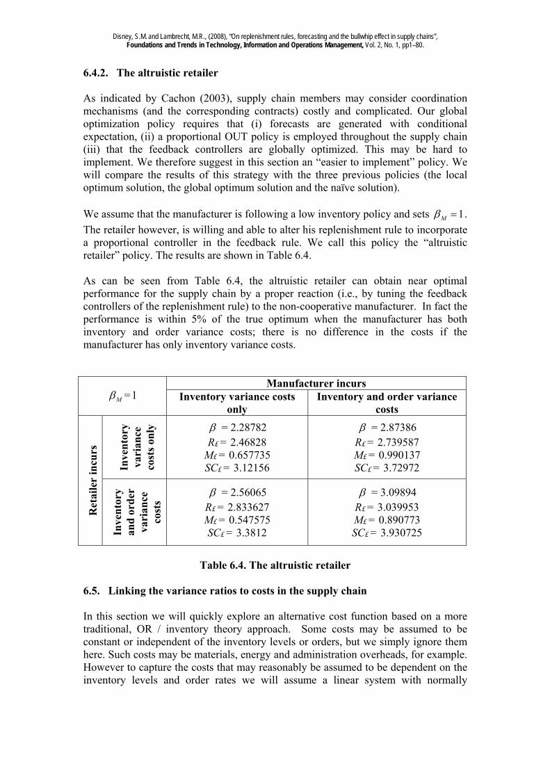
On replenishment rules, forecasting and the bullwhip ... - On replenishment rules... · Disney,...

Disney, S.M. and Lambrecht, M.R., (2008), “On replenishment rules, forecasting and the bullwhip effect in supply chains”, Foundations and Trends in Technology, Information and Operations Management, Vol. 2, No. 1, pp1–80.

On replenishment rules, forecasting and the bullwhip effect in supply chains

Stephen M. Disney1 and Marc R. Lambrecht2

1 Logistics Systems Dynamics Group, Cardiff Business School, Cardiff University, Aberconway

Building, Colum Drive, Cardiff, CF10 3EU, UK. Email: [email protected].

2 Research Center for Operations Management, Katholieke Universiteit Leuven, Naamsestraat 69, 3000

Leuven, Belgium. Email: [email protected].

1. Modern supply chains Supply chains are networks of firms who pool their capabilities and resources in order to deliver value to the end consumer. Firms are no longer able to own or control complete supply chains. Information technology and modern logistics capabilities have created a global market where companies can take advantage of the opportunity to source internationally (IBM Business Consulting Services 2005). Companies have thus specialized and to “partnered” globally with other companies. These companies have then to increasingly focus on logistics and supply chain co-ordination. Such co-ordination is now an essential business process. Modern supply chain management starts with the premise that supply chain members are primarily concerned with optimizing their own objectives and this self-serving focus often results in poor performance. Another way of saying this is that a sequence of local optimum policies does not bring about a globally optimum solution, Cachon (2003). Munson et al. (2003) summarize it as follows “When each member of a group tries to maximize his or her own benefit without regard to the impact on other members of the group, the overall effectiveness may suffer. Such inefficiencies often creep in when rational members of supply chains optimize individually instead of coordinating their efforts”. A well known example of such inefficiency is the bullwhip effect. This effect refers to the tendency of replenishment orders to increase in variability as one moves up the supply chain from retailer to manufacturer. A disintegrated material flow, combined with distorted demand information and a lack of replenishment rule alignment inevitably results in a poor supply chain dynamics. This lack of coordination may even outweigh the benefits from specialization and economies of scale. In this monograph we will focus on supply chain co-ordination and we use the bullwhip effect as the key example of supply chain inefficiency. We focus both on the managerial relevance of the bullwhip effect, but we also emphasize on the methodological issues so that both managers and researchers alike can benefit from reading this monograph.


2. The bullwhip effect: The dynamics of supply chains The “bullwhip effect” is short-hand term for a dynamical phenomenon in supply chains. It refers to the tendency of the variability of order rates to increase as they pass through the echelons of a supply chain towards producers and raw material suppliers. 2.1 Empirical evidence of bullwhip There is ample anecdotic evidence that many companies experience significant extra costs due to supply chain problems. Konicki (2002) reports on a major retailer’s inability to master supply chain logistical problems. The company faced sharp spikes and drops in demand for products and sales merchandise was often out of stock when customers got to the store. Furthermore, bloated stocks sat alongside these empty racks and display shelves, but they were no guarantee of high customer service levels. It is a formidable job for logistics managers to design order management systems that optimally match pipelines to the marketplace (see Looman, Ruttins and de Boer (2002), Childerhouse, Aitken and Towill (2002) and Christopher and Towill (2002)). What is causing all this trouble? Why is it that the material flow is so hard to predict in supply networks? There are for sure many causes of these deficiencies. In this monograph we will focus on the bullwhip effect. The bullwhip problem refers to the tendency of replenishment orders to increase in variability as one moves up a supply chain. As smooth final customer demand patterns are transformed into highly erratic demand patterns for suppliers, the information in the chain gets distorted. The bullwhip is characterised by oscillations of orders at each level of the supply chain and an amplification of these oscillations as one moves farther away from the customer (Croson and Donohue (2003)). Jay Forrester (1961) was among the first researchers to describe this phenomenon, who then called the effect “demand amplification”. A number of researchers designed games to illustrate the bullwhip effect. The most famous game is the “Beer Distribution Game”. This game has a rich history. Growing out of the industrial dynamics work of Forrester and others at MIT, it is later on developed by Sterman (1989). The Beer Game is by far the most popular simulation and the most widely used game in many business schools, supply chain electives and executive seminars. Simchi-Levi et al. (1998) developed a computerized version of the beer game, and several versions of the beer game are now available, ranging from manual to computerized and even web-based versions, for example see http://beergame.mit.edu/default.htm, Machuca and Barajas (1997), Chen and Samroengraja (2000) and Jacobs (2000). Others versions have been adapted to represent particular industries Van Horne and Marier (2007) or to investigate particular supply chain strategies such as information sharing or VMI, Disney, Naim and Potter (2004). Beyond the games, real cases are used as teaching tools to introduce and to address the bullwhip effect (Lee et al. 2004). The Barilla SpA case study (Hammond, 1994), a major pasta producer in Italy, provides vivid illustrations of issues concerning the bullwhip effect. For a long time Barilla offered special price discounts to customers who ordered full truckload quantities. Such marketing deals created customer order


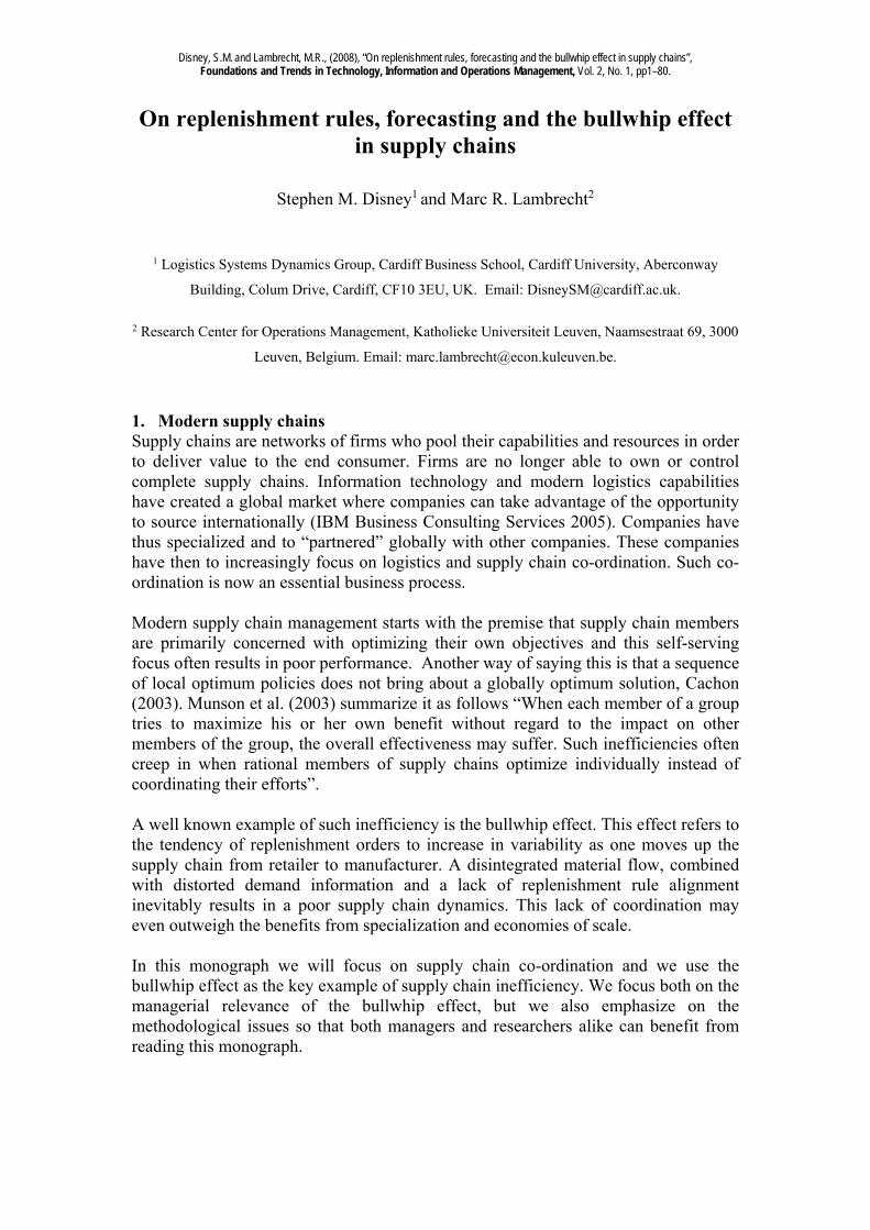
patterns that were highly spiky and erratic. The supply chain costs were so high that they outstripped the benefits from full truckload transportation. The Barilla case was one of the first published cases that empirically supported the bullwhip phenomenon. Campbell Soup’s chicken noodle soup experience, Cachon and Fisher (1997) is another example. Campbell Soup sells products whose customer demand is fairly stable. The consumption of their products doesn’t swing wildly from week to week, although there is an annual cycle. Yet the manufacturer faced extremely variable demand on the factory level. After some investigation, they found that the wide swings in demand were caused by the ordering practices of retailers. The swing was induced by forward buying. More recent teaching cases that address the bullwhip effect include Kuper and Branvold (2000), Hoyt (2001) and Peleg (2003).

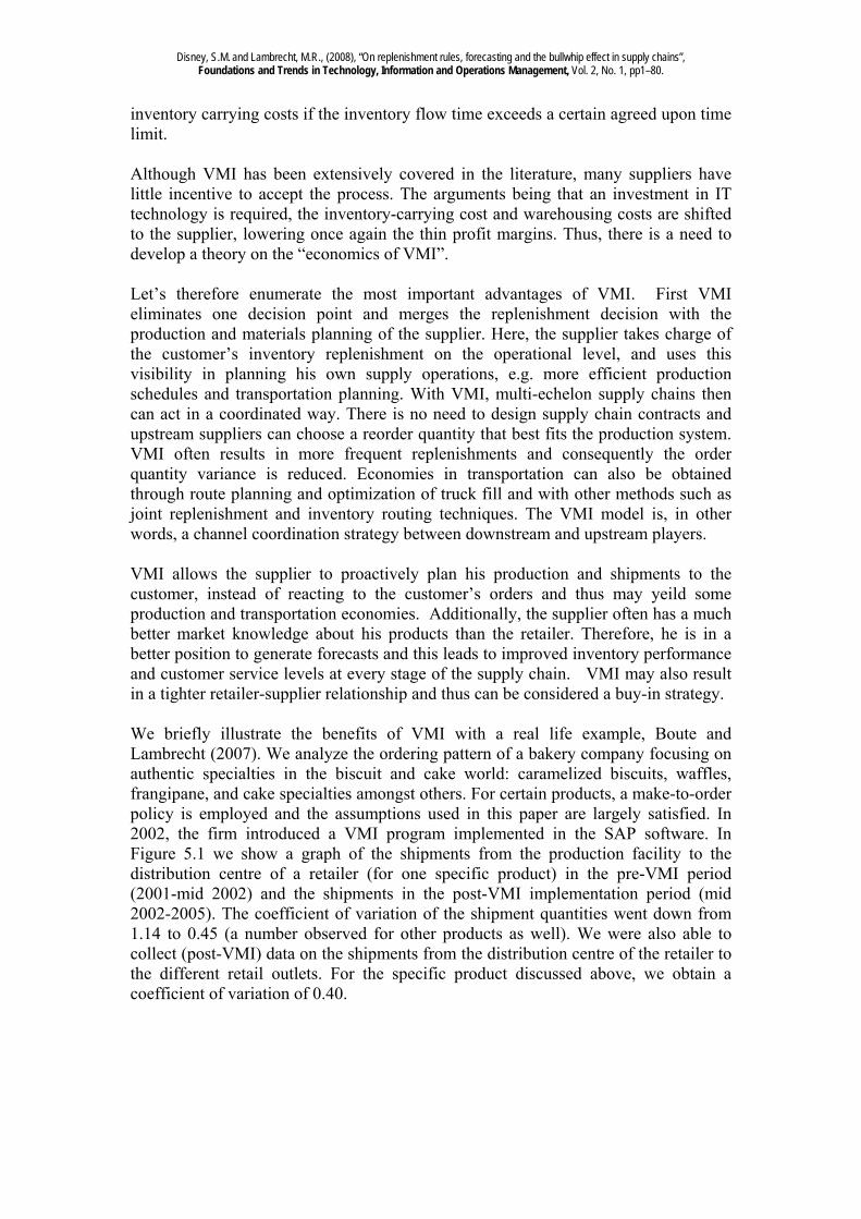
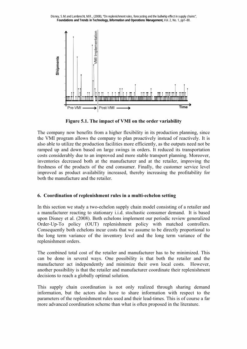
Figure 2.1. The Campbell Soup promotion Source: Cachon and Fisher, (1997)

The classic example of the bullwhip effect is baby nappies or diapers. Indeed Procter and Gamble first coined the phrase “bullwhip effect” to describe the ordering behaviour witnessed between customers and suppliers of diapers. Babies are fairly regular in their use of nappies - they have a new nappy (almost) every time they feed. Sure, there is seasonal variation in the birth rates as more babies are conceived in spring (when male sperm count is significantly higher than in any other season; however this is not globally consistent and the there is some debate over the role of both temperature and the day length, Lam and Miron (1996)). Neither-the-less, this seasonal variation is small compared to the widely fluctuating and erratic production rates experienced by P&G after the orders have passed through the supermarkets and distribution centres. P&G observed a further amplification of the oscillations of orders placed to their suppliers of raw material. Our own data from a large leading consumer packaged goods firm, shows that the coefficient of variation (the ratio of the standard deviation over the mean) of retail sales typically ranges between 0.15 and 0.50 whereas the coefficient of variation of


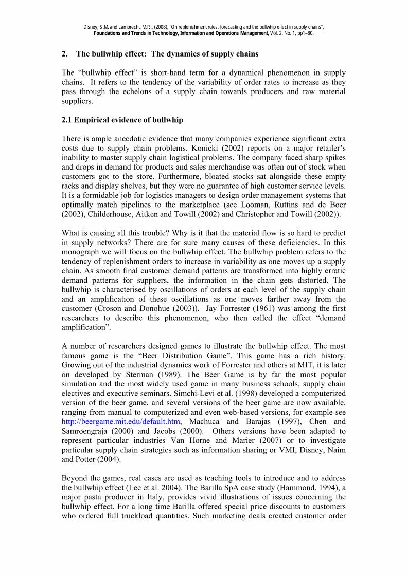
production orders (even in small batch driven environments) is typically in the range of 2 to 3. Moreover, the bullwhip effect is multiplicative in traditional supply chains. Holweg et al. (2005) examined a grocery retail chain, where the actual demand signal from the customers in the supermarket for a soft drink is amplified many times before it reaches the soft drink supplier. The largest weekly order placed on the supplier is five times the average weekly sales volume in the supermarkets. The coefficient of variation also depends on the level of aggregation. The coefficient of variation based on daily data is much larger than the coefficient of variation based on weekly or monthly date. The same holds for coefficients of variation for individual products compared to coefficients of variations for aggregate demands or shipments. Measuring the bullwhip effect is, in other words, a difficult job. One can start with Point of Sales data for individual products for one specific retail outlet. Next the demand is aggregated on the retailer distribution centre and further aggregated at the manufacturer’s distribution centre. Finally we reach the production facility. This complex process of aggregation (through replenishment rules, manufacturing batch sizes, full truck load transportation policies, amongst others) makes the bullwhip effect analysis very hard. This explains why most research focuses on replenishment rules for individual items on the retail outlet level. Let’s conclude this section on empirical evidence with an example of a large manufacturer of indoor and outdoor lighting products. This company is active in almost all European countries and they have production facilities mainly in Eastern Europe and China. We distinguish two types of sales organizations: large sales organizations (mainly Western European countries and large volume sales) and small sales organizations (mainly Eastern European countries and smaller volume sales items). There are two distribution centres - Central Services (CS) and Local Services (LS). The CS distribution centre receives orders from the large sales organisations and delivers the products to the large sales organizations very frequently. LS receives orders from the small sales organizations and LS is replenished through CS. Deliveries to the small sales organizations and shipments from CS to LS are less frequent.

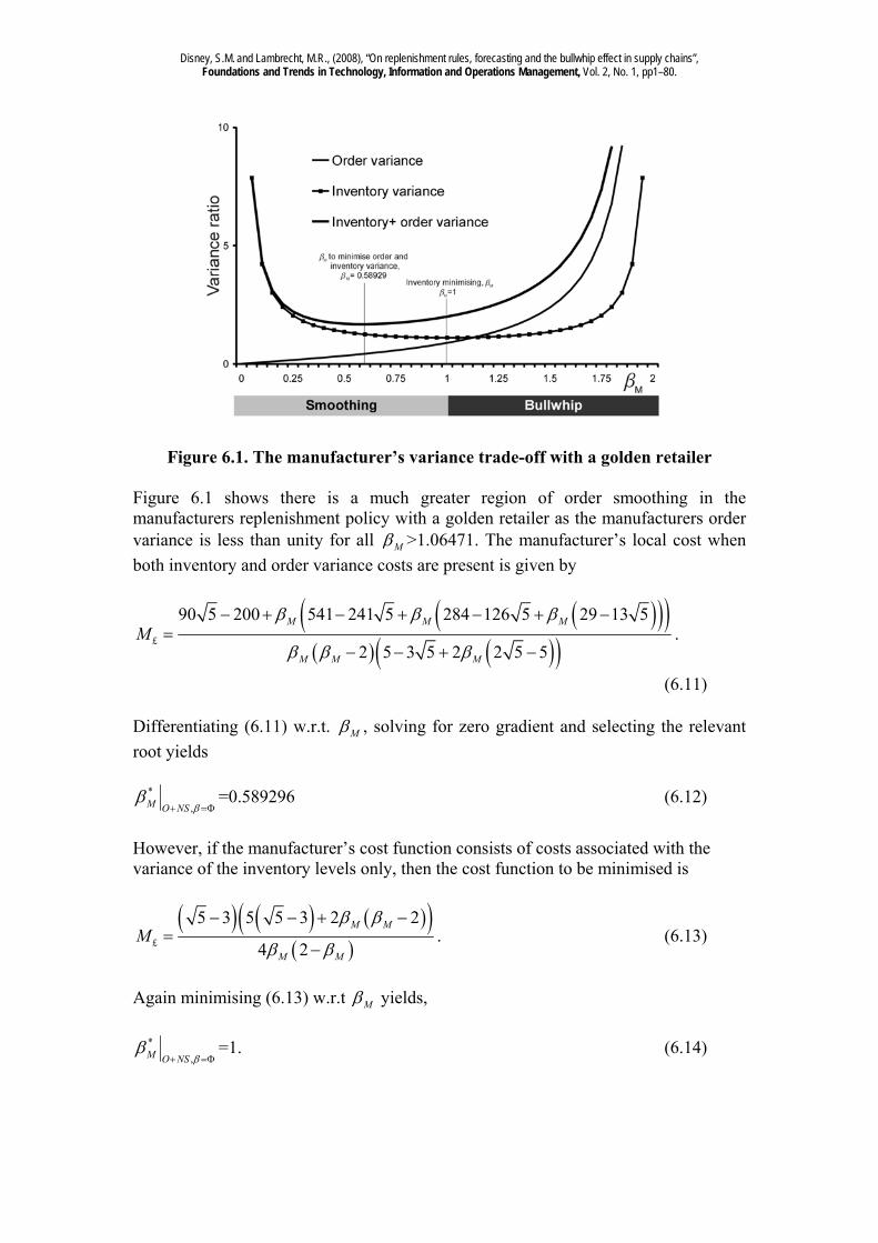
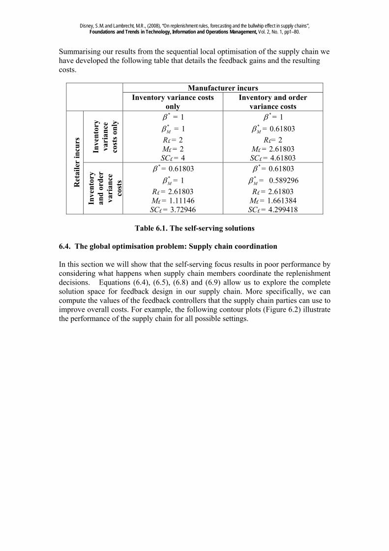
Figure 2.2. Bullwhip in the light bulb supply chain


We analyzed the material flow of products ordered by the small sales organizations. We collected sales data on a weekly basis and computed the coefficient of variation (CV). The average CV is 0.76. We also have data of weekly shipments from LS to the local warehouses of the small sales organizations (there is no aggregation problem because the small sales organizations do not have a central distribution centre). The average CV equals 1.20. Finally we analyzed the shipments from CS to LS. Here the demand for an individual product is aggregated over all (small) markets and still, the CV of weekly shipments equals 2.21. There is clearly a bullwhip effect. The bullwhip effect however is absent or far less outspoken for the large sales organizations because CS is regularly allocating products to the large sales organization on a fair share allocation basis and cross docks the production volumes received. 2.2. Causes of the bullwhip effect We will now review causes of the bullwhip effect as mentioned in the literature, and investigate ways to alleviate and to overcome the problem. We distinguish operational and behavioural causes. The behavioural causes are rather straightforward. Supply chain managers may not always be completely rational. Managers over-react (or under-react) to demand changes. People often try to read “too much signal” into a series of demand history as it changes over time. Often people are over optimistic and confuse forecasts with targets. Decision makers sometimes over-react to customer complaints and anecdotes of negative customer reactions. Moreover, there are cognitive limitations as supply chain networks are often very complicated, operating in a highly uncertain environment with limited access to data. Croson and Donohue (2002) and Sterman (1989) found that decision makers consistently under-weight the supply chain. This means that they don’t have a clear idea of what is available in the pipeline. This induces some form of decision bias. Strategies to alleviate this problem include; sharing Point-Of-Sales data, sharing inventory and demand information, centralizing ordering decisions and using formal forecasting techniques correctly (we will come back on this issue later on in this monograph). Lee et al. (1997a and 1997b) identify five major operational causes of the bullwhip: demand signal processing, lead-time, order batching, price fluctuations and rationing and shortage gaming. We understand demand signal processing as the practice of decision makers adjusting the parameters of the inventory replenishment rule. Target stock levels, safety stocks and demand forecasts are updated in face of new information or deviations from targets. These “rational” adjustments create erratic responses. We will also show that it is possible to design replenishment rules that have a stabilizing, smoothing effect on orders. It is important to realize that most players in supply chains do not respond directly to the market but respond to replenishment demand from downstream echelons. This is why local optimisation often results in global disharmony. It is therefore claimed that centralized control (e.g. Distribution Requirements Planning, Vendor Managed Inventory, for example) is superior to decentralized control. A second major cause of the bullwhip problem is the lead-time. Lead-times are made of two components; the physical delays as well as the information delays. The lead-time is a key parameter for calculating safety stock, reorder points and order-up-to


levels. The increase in variability is magnified with increasing lead-time. A way to alleviate this problem is lead-time compression. The information delay can be reduced by better communication technologies (web-enabled communication, EDI, e-procurement etc) and the order fulfilment lead-time (the physical lead-time) can be reduced by investment in production technology, strategic supplier partnerships (supplier hubs, logistics integrators etc) or by eliminating channel intermediaries (direct channels, ‘the Dell model’). The information delay should never be taken for granted. In a three echelon UK grocery supply chain with all the modern IT technology, the information delay is still of the same magnitude as the material delays; 16 days for information to flow up four echelons of the supply chain, 19 days for material to flow down. In this monograph we will mainly focus on these two causes of the bullwhip, demand signal processing and lead-times. A third well-known bullwhip creator is the practice of order batching. Economies of scale in ordering, production set-ups or transportation will quite clearly increase order variability. Reduction of set-up, ordering and handling costs is of course a way to alleviate this problem. Potter and Disney (2006) have also shown that setting the batch size so that multiples of the batch quantity matches the average demand results in reduced bullwhip measures. Holland and Sodhi (2004) use simulation to show the order variance is proportional to the square of the batch size and the demand variation. John Burbidge was also aware of the batching effects and developed a range of practical approaches to the problem as far back as the 1960’s, Towill (1994). The fourth major cause of bullwhip as highlighted by Lee et al. (1997a and 1997b) has to do with price fluctuations. Retailers often offer price discounts, quantity discounts, coupons or in-store promotions. This results in forward buying where retailers (as well as consumers) buy in advance and in quantities that do not reflect their immediate needs. Pricing strategies (ranging from deep promotions to Every Day Low Price) should clearly be connected to supply and replenishment policies. However, it is not sure from a marketing perspective whether the positive supply chain effect (higher efficiencies) outweighs the potential negative marketing effect (demand-depressing side effects). We refer to Ortmeyer et al. (1991) and Butman (2002) for more details on issues in the operations management and marketing interface.


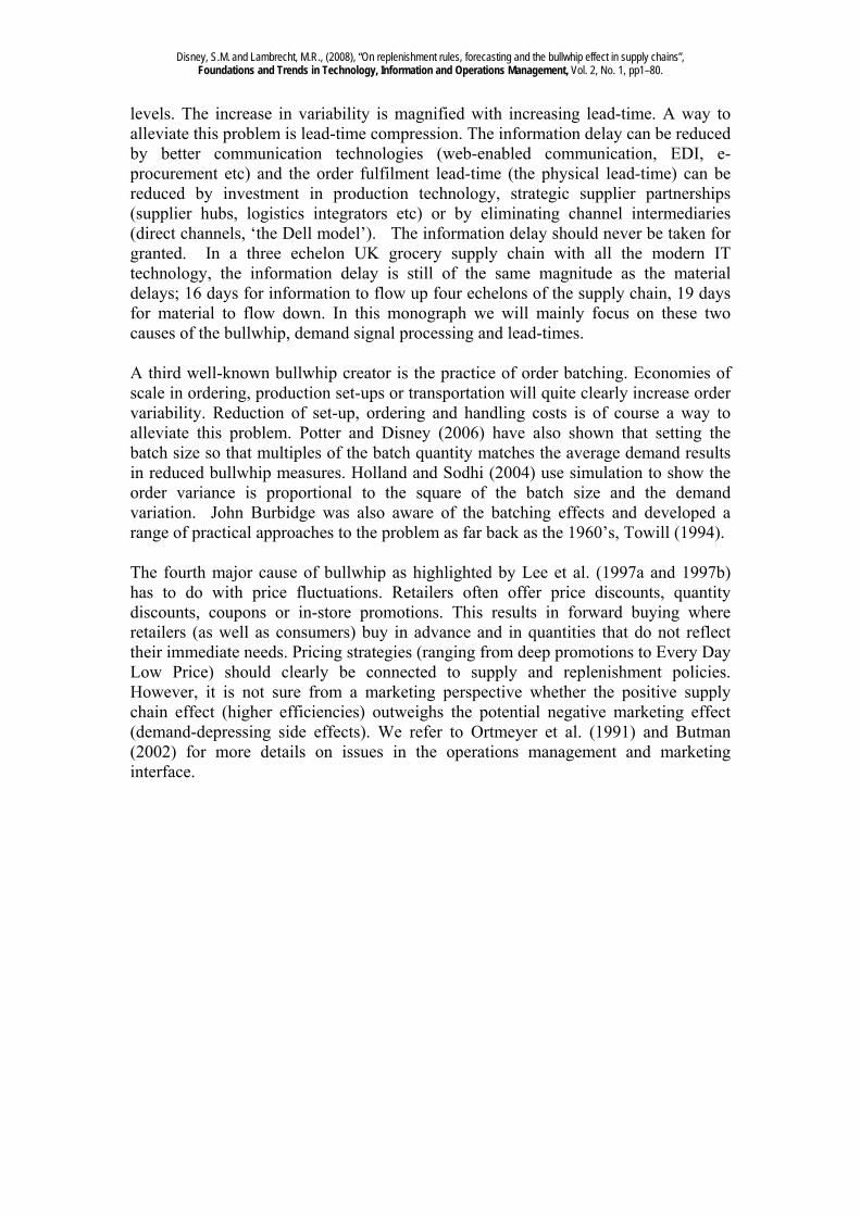
Figure 2.3. The causes of the bullwhip effect (The focus of this monograph is highlighted in grey)

In general, it is important to transmit the correct demand information into the supply chain. An accurate forecast (see Chen, Drezner, Ryan and Simchi-Levi (2000)) will assist the upstream suppliers’ capacity and material planning. Furthermore, inventory requirements are directly linked to the errors between the forecast of demand over the lead-time and review period and the actual realisation of demand, Vassian (1955). We may want to stimulate forecast accuracy and to penalise forecast errors. Thus, we may want to limit the ability to revise forecasts over time, or we may negotiate flexibility contracts with customers (based on risk sharing). These are all ways to manipulate demand and to view forecasting as more than just a courtesy. A further cause of bullwhip is connected with rationing and shortage gaming. Inflated orders placed by supply chain members during shortage periods tend to magnify the bullwhip effect. Such orders are common when retailers and distributors suspect that a product will be in short supply. Exaggerated customers orders make it hard for manufacturers to forecast the real demand level. A very simple countermeasure is to allocate products proportional to sales in previous periods and rather than allocating based on what has been ordered. This short overview of the causes of the bullwhip effect (and a short summary of potential remedies) highlights that the bullwhip effect is a very complex issue. It touches on all aspects of supply chain management. 2.3. The link between the bullwhip effect and supply chain costs Bullwhip creates unstable production schedules. These unstable production schedules are the cause of a range of unnecessary costs in supply chains. Companies have to invest in extra capacity to meet the highly variable demand. This capacity is then under-utilised when demand drops. Unit labour costs rise in periods of low demand, over-time, agency and sub-contract costs rise in periods of high demand. The highly


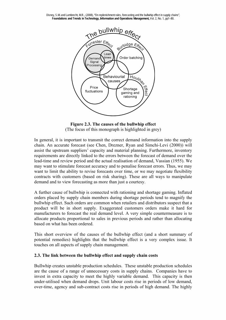
variable demand increases the requirements for safety stock in the supply chain. Additionally, companies may decide to produce to stock in periods of low demand to increase productivity. If this is not managed properly this will lead to excessive obsolescence. Highly variable demand also increases lead-times. These inflated lead-times lead to increased stocks and bullwhip effects. Thus the bullwhip effect can be quite exasperating for companies; they invest in extra capacity, extra inventory, work over-time one week and stand idle the next, whilst at the retail store the shelves of popular products are empty, and the shelves with products that aren’t selling are full. A cause and effect diagram in Figure 2.4 highlights the interaction between demand variance and cost generation.

Figure 2.4. How bullwhip creates costs in a single echelon of a supply chain Inventory managers must consider two primary factors when making replenishment decisions. First, a replenishment rule has an impact on order variability (as measured by the bullwhip effect, that is, the ratio of the variance of orders over the variance of demand) shown to the supplier. Second, the replenishment rule has an impact on the variance of the net stock (as measured by the net stock amplification, the ratio of net stock variance over the variance of demand). The bullwhip effect mainly contributes to upstream costs, while the variance of net stock determines the stage’s ability to meet a service level in a cost-effective manner. This is the key trade-off faced by a single-stage member of a supply chain. It is interesting to note that the problem described above may lead to non-cooperative behaviour. Indeed, the bullwhip effect is driving costs at the upstream stage (for example the manufacturer or supplier) and consequently, the downstream stage (for example the retailer) may not worry about it. Even worse, dampening the bullwhip effect may have a negative impact on customer service at the retailer. So why should a downstream stage be concerned with upstream costs? The key to this question is that the retailer will still have some distribution activities (warehouses, transportation, receiving goods at stores, for example) and he will care about the efficiency of these processes. Furthermore the retailer may be able to secure more cost reductions from a supplier by placing smoother demands as these smooth demands will allow the supplier to reduce his costs. Thirdly, there maybe a lead-time effect, as smooth demand allows manufacturers to respond with a quicker lead-time, Boute et al. (2007). Thus, we need some measures of performance for the bullwhip effect. A simple metric that often results naturally from an analysis of how the bullwhip effect is


generated is the also called “variance ratio” we have mentioned, see Equation (2.1). Indeed this is by far the most common bullwhip measure in the literature.

)(

)(2

2

DemandVar

OrdersVarBullwhip

Demand

Orders

(2.1)

A bullwhip measure equal to one implies that the order variance is equal to the demand variance, or in other words, there is no variance amplification. A bullwhip larger than one indicates that the bullwhip effect is present (amplification), whereas a bullwhip smaller than one is referred to as a “smoothing” scenario, meaning that the orders are smoothed (less variable) compared to the demand pattern (dampening). Our focus, however is not solely on the bullwhip measure. We also check the variance of the net stock since this has a significant impact on customer service (the higher the variance of net stock, the more safety stock required). Thus the following metric is also important.

2

2

( )

( )Net Stock

Demand

Var Net StockNSAmp

Var Demand

(2.2)

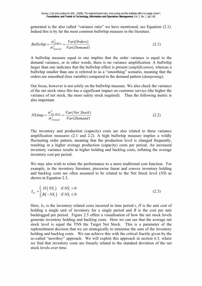
The inventory and production (capacity) costs are also related to these variance amplification measures (2.1 and 2.2). A high bullwhip measure implies a wildly fluctuating order pattern, meaning that the production level is changed frequently, resulting in a higher average production (capacity) costs per period. An increased inventory variance results in higher holding and backlog costs, inflating the average inventory cost per period. We may also wish to relate the performance to a more traditional cost function. For example, in the inventory literature, piecewise linear and convex inventory holding and backlog costs are often assumed to be related to the Net Stock level (NS) as shown in Equation 2.3,

$,

if 0

if 0t t

tt t

H NS NSI

B NS NS

(2.3)

Here, I$,t is the inventory related costs incurred in time period t, H is the unit cost of holding a single unit of inventory for a single period and B is the cost per unit backlogged per period. Figure 2.5 offers a visualisation of how the net stock levels generate inventory holding and backlog costs. Here we can see that the average net stock level is equal the TNS the Target Net Stock. This is a parameter of the replenishment decision that we set strategically to minimise the sum of the inventory holding and backlog costs. We can achieve this with the critical fractile given by the so-called “newsboy” approach. We will exploit this approach in section 6.5, where we find that inventory costs are linearly related to the standard deviation of the net stock levels over time.


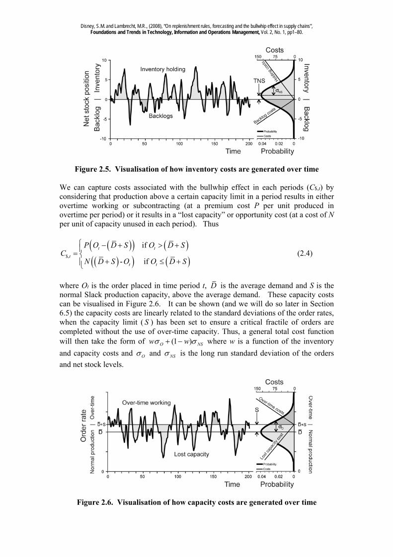
Figure 2.5. Visualisation of how inventory costs are generated over time We can capture costs associated with the bullwhip effect in each periods (C$,t) by considering that production above a certain capacity limit in a period results in either overtime working or subcontracting (at a premium cost P per unit produced in overtime per period) or it results in a “lost capacity” or opportunity cost (at a cost of N per unit of capacity unused in each period). Thus

$,

if

- if

t t

t

t t

P O D S O D SC

N D S O O D S

(2.4)

where Ot is the order placed in time period t, D is the average demand and S is the normal Slack production capacity, above the average demand. These capacity costs can be visualised in Figure 2.6. It can be shown (and we will do so later in Section 6.5) the capacity costs are linearly related to the standard deviations of the order rates, when the capacity limit ( S ) has been set to ensure a critical fractile of orders are completed without the use of over-time capacity. Thus, a general total cost function will then take the form of NSO ww )1( where w is a function of the inventory

and capacity costs and O and NS is the long run standard deviation of the orders

and net stock levels.

Figure 2.6. Visualisation of how capacity costs are generated over time


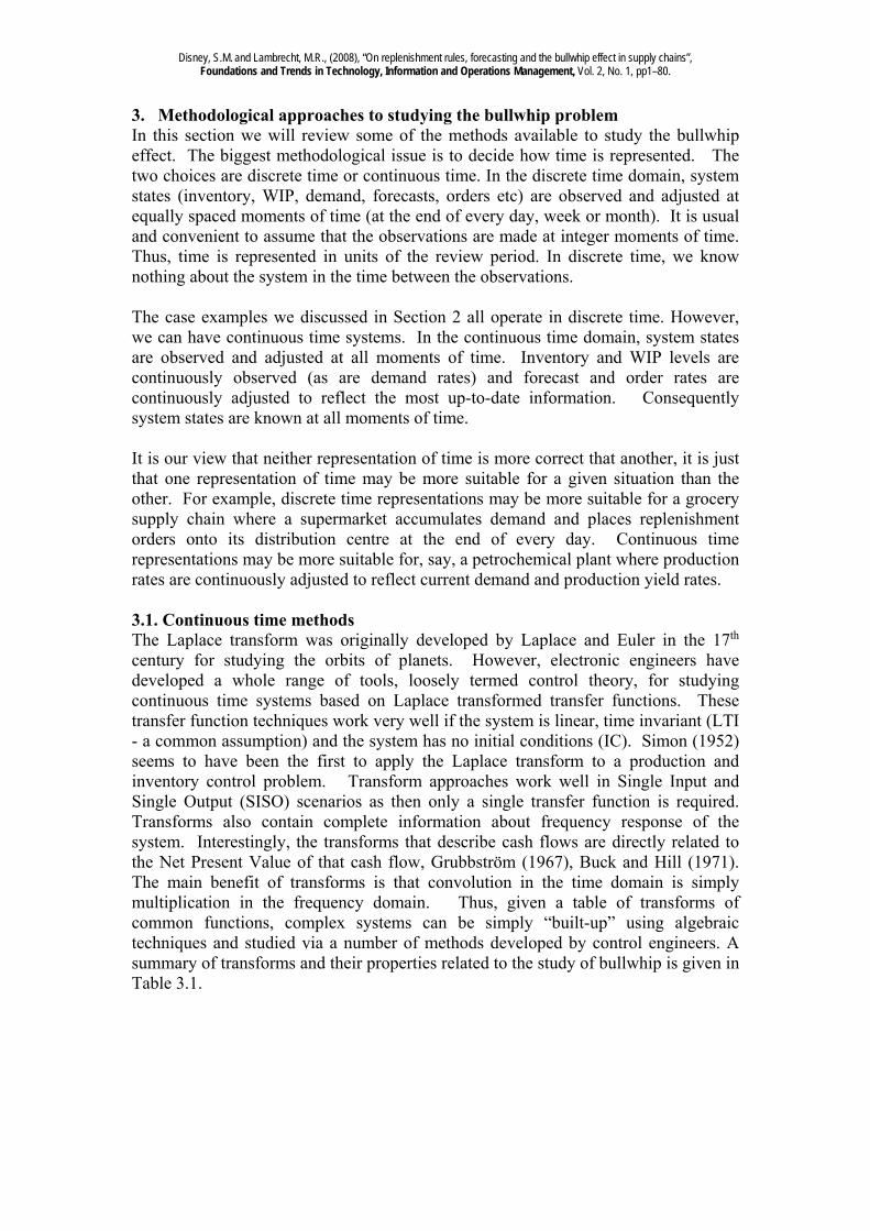
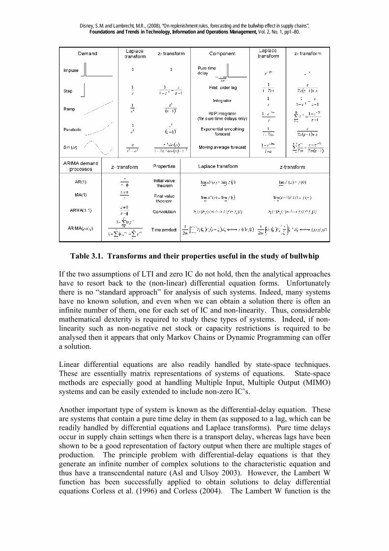
3. Methodological approaches to studying the bullwhip problem In this section we will review some of the methods available to study the bullwhip effect. The biggest methodological issue is to decide how time is represented. The two choices are discrete time or continuous time. In the discrete time domain, system states (inventory, WIP, demand, forecasts, orders etc) are observed and adjusted at equally spaced moments of time (at the end of every day, week or month). It is usual and convenient to assume that the observations are made at integer moments of time. Thus, time is represented in units of the review period. In discrete time, we know nothing about the system in the time between the observations. The case examples we discussed in Section 2 all operate in discrete time. However, we can have continuous time systems. In the continuous time domain, system states are observed and adjusted at all moments of time. Inventory and WIP levels are continuously observed (as are demand rates) and forecast and order rates are continuously adjusted to reflect the most up-to-date information. Consequently system states are known at all moments of time. It is our view that neither representation of time is more correct that another, it is just that one representation of time may be more suitable for a given situation than the other. For example, discrete time representations may be more suitable for a grocery supply chain where a supermarket accumulates demand and places replenishment orders onto its distribution centre at the end of every day. Continuous time representations may be more suitable for, say, a petrochemical plant where production rates are continuously adjusted to reflect current demand and production yield rates. 3.1. Continuous time methods The Laplace transform was originally developed by Laplace and Euler in the 17th century for studying the orbits of planets. However, electronic engineers have developed a whole range of tools, loosely termed control theory, for studying continuous time systems based on Laplace transformed transfer functions. These transfer function techniques work very well if the system is linear, time invariant (LTI - a common assumption) and the system has no initial conditions (IC). Simon (1952) seems to have been the first to apply the Laplace transform to a production and inventory control problem. Transform approaches work well in Single Input and Single Output (SISO) scenarios as then only a single transfer function is required. Transforms also contain complete information about frequency response of the system. Interestingly, the transforms that describe cash flows are directly related to the Net Present Value of that cash flow, Grubbström (1967), Buck and Hill (1971). The main benefit of transforms is that convolution in the time domain is simply multiplication in the frequency domain. Thus, given a table of transforms of common functions, complex systems can be simply “built-up” using algebraic techniques and studied via a number of methods developed by control engineers. A summary of transforms and their properties related to the study of bullwhip is given in Table 3.1.


Table 3.1. Transforms and their properties useful in the study of bullwhip If the two assumptions of LTI and zero IC do not hold, then the analytical approaches have to resort back to the (non-linear) differential equation forms. Unfortunately there is no “standard approach” for analysis of such systems. Indeed, many systems have no known solution, and even when we can obtain a solution there is often an infinite number of them, one for each set of IC and non-linearity. Thus, considerable mathematical dexterity is required to study these types of systems. Indeed, if non-linearity such as non-negative net stock or capacity restrictions is required to be analysed then it appears that only Markov Chains or Dynamic Programming can offer a solution. Linear differential equations are also readily handled by state-space techniques. These are essentially matrix representations of systems of equations. State-space methods are especially good at handling Multiple Input, Multiple Output (MIMO) systems and can be easily extended to include non-zero IC’s. Another important type of system is known as the differential-delay equation. These are systems that contain a pure time delay in them (as supposed to a lag, which can be readily handled by differential equations and Laplace transforms). Pure time delays occur in supply chain settings when there is a transport delay, whereas lags have been shown to be a good representation of factory output when there are multiple stages of production. The principle problem with differential-delay equations is that they generate an infinite number of complex solutions to the characteristic equation and thus have a transcendental nature (Asl and Ulsoy 2003). However, the Lambert W function has been successfully applied to obtain solutions to delay differential equations Corless et al. (1996) and Corless (2004). The Lambert W function is the


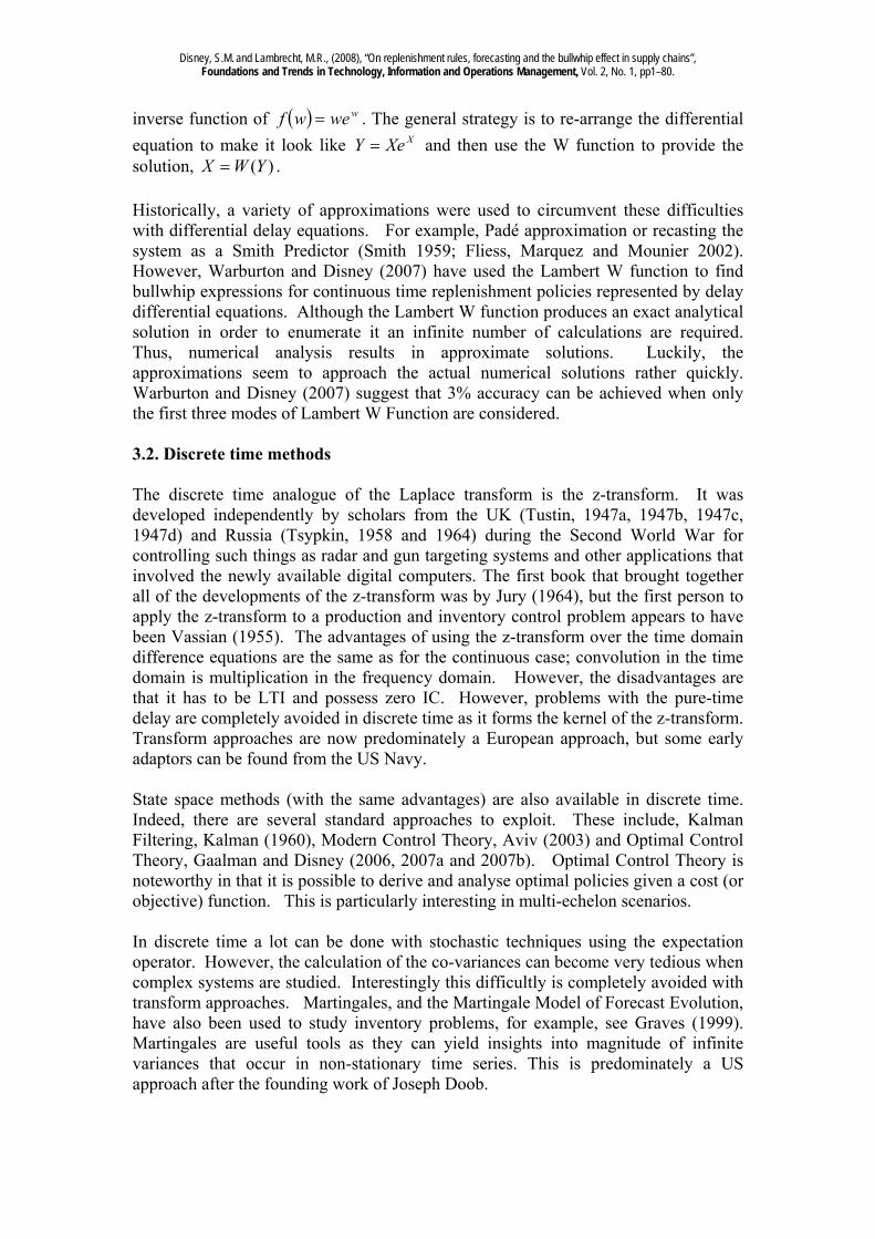
inverse function of wwewf . The general strategy is to re-arrange the differential

equation to make it look like XXeY and then use the W function to provide the solution, )(YWX . Historically, a variety of approximations were used to circumvent these difficulties with differential delay equations. For example, Padé approximation or recasting the system as a Smith Predictor (Smith 1959; Fliess, Marquez and Mounier 2002). However, Warburton and Disney (2007) have used the Lambert W function to find bullwhip expressions for continuous time replenishment policies represented by delay differential equations. Although the Lambert W function produces an exact analytical solution in order to enumerate it an infinite number of calculations are required. Thus, numerical analysis results in approximate solutions. Luckily, the approximations seem to approach the actual numerical solutions rather quickly. Warburton and Disney (2007) suggest that 3% accuracy can be achieved when only the first three modes of Lambert W Function are considered. 3.2. Discrete time methods The discrete time analogue of the Laplace transform is the z-transform. It was developed independently by scholars from the UK (Tustin, 1947a, 1947b, 1947c, 1947d) and Russia (Tsypkin, 1958 and 1964) during the Second World War for controlling such things as radar and gun targeting systems and other applications that involved the newly available digital computers. The first book that brought together all of the developments of the z-transform was by Jury (1964), but the first person to apply the z-transform to a production and inventory control problem appears to have been Vassian (1955). The advantages of using the z-transform over the time domain difference equations are the same as for the continuous case; convolution in the time domain is multiplication in the frequency domain. However, the disadvantages are that it has to be LTI and possess zero IC. However, problems with the pure-time delay are completely avoided in discrete time as it forms the kernel of the z-transform. Transform approaches are now predominately a European approach, but some early adaptors can be found from the US Navy. State space methods (with the same advantages) are also available in discrete time. Indeed, there are several standard approaches to exploit. These include, Kalman Filtering, Kalman (1960), Modern Control Theory, Aviv (2003) and Optimal Control Theory, Gaalman and Disney (2006, 2007a and 2007b). Optimal Control Theory is noteworthy in that it is possible to derive and analyse optimal policies given a cost (or objective) function. This is particularly interesting in multi-echelon scenarios. In discrete time a lot can be done with stochastic techniques using the expectation operator. However, the calculation of the co-variances can become very tedious when complex systems are studied. Interestingly this difficultly is completely avoided with transform approaches. Martingales, and the Martingale Model of Forecast Evolution, have also been used to study inventory problems, for example, see Graves (1999). Martingales are useful tools as they can yield insights into magnitude of infinite variances that occur in non-stationary time series. This is predominately a US approach after the founding work of Joseph Doob.


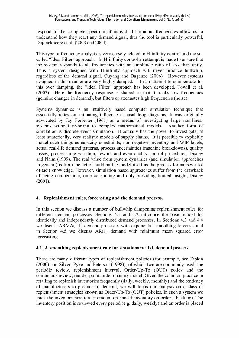
A particularly useful difference equation approach was developed by Box and Jenkins (1970). Known as ARIMA modelling, Box and Jenkins developed a generalised time series model that consisted of an arbitrary number of three types of terms. That is, Auto-Regressive, Integrated and Moving Average terms. The general ARIMA(p,d,q) model is given by Equation 3.1. The Box and Jenkins approach copes with non-stationary processes by differencing the time series.

noise White

termsAverage Moving

1

termseIntegrativ

1

termsRegressive Auto

1t

q

kktk

d

jjt

p

iitit DDD

(3.1)

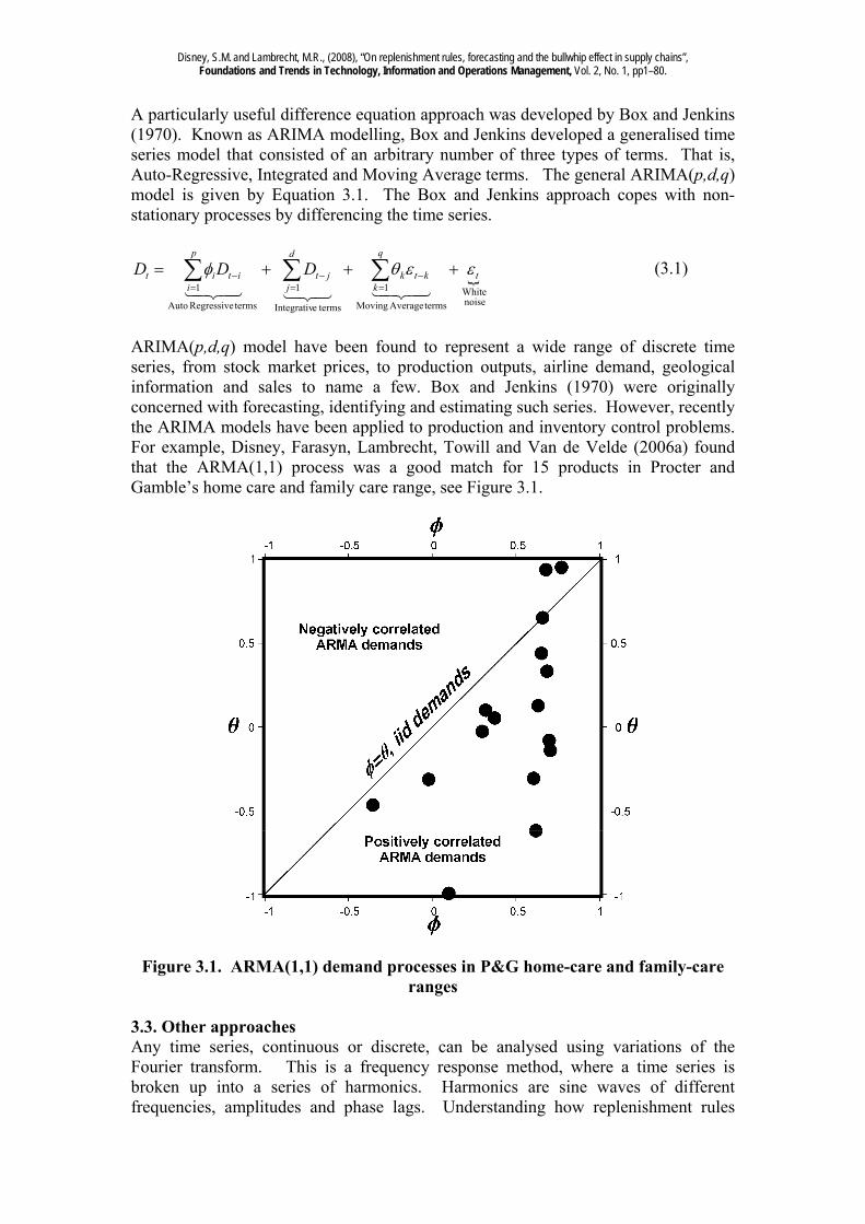
ARIMA(p,d,q) model have been found to represent a wide range of discrete time series, from stock market prices, to production outputs, airline demand, geological information and sales to name a few. Box and Jenkins (1970) were originally concerned with forecasting, identifying and estimating such series. However, recently the ARIMA models have been applied to production and inventory control problems. For example, Disney, Farasyn, Lambrecht, Towill and Van de Velde (2006a) found that the ARMA(1,1) process was a good match for 15 products in Procter and Gamble’s home care and family care range, see Figure 3.1.

Figure 3.1. ARMA(1,1) demand processes in P&G home-care and family-care ranges

3.3. Other approaches Any time series, continuous or discrete, can be analysed using variations of the Fourier transform. This is a frequency response method, where a time series is broken up into a series of harmonics. Harmonics are sine waves of different frequencies, amplitudes and phase lags. Understanding how replenishment rules


respond to the complete spectrum of individual harmonic frequencies allow us to understand how they react any demand signal, thus the tool is particularly powerful, Dejonckheere et al. (2003 and 2004). This type of frequency analysis is very closely related to H-infinity control and the so-called “Ideal Filter” approach. In H-infinity control an attempt is made to ensure that the system responds to all frequencies with an amplitude ratio of less than unity. Thus a system designed with H-infinity approach will never produce bullwhip, regardless of the demand signal, Ouyang and Daganzo (2006). However systems designed in this manner are very highly damped. In an attempt to compensate for this over damping, the “Ideal Filter” approach has been developed, Towill et al. (2003). Here the frequency response is shaped so that it tracks low frequencies (genuine changes in demand), but filters or attenuates high frequencies (noise). Systems dynamics is an intuitively based computer simulation technique that essentially relies on animating influence / causal loop diagrams. It was originally advocated by Jay Forrester (1961) as a means of investigating large non-linear systems without resorting to complex mathematical models. Another form of simulation is discrete event simulation. It actually has the power to investigate, at least numerically, very realistic models of supply chains. It is possible to explicitly model such things as capacity constraints, non-negative inventory and WIP levels, actual real-life demand patterns, process uncertainties (machine breakdowns), quality losses, process time variation, rework and even quality control procedures, Disney and Naim (1999). The real value from system dynamics (and simulation approaches in general) is from the act of building the model itself as the process formalises a lot of tacit knowledge. However, simulation based approaches suffer from the drawback of being cumbersome, time consuming and only providing limited insight, Disney (2001). 4. Replenishment rules, forecasting and the demand process. In this section we discuss a number of bullwhip dampening replenishment rules for different demand processes. Sections 4.1 and 4.2 introduce the basic model for identically and independently distributed demand processes. In Sections 4.3 and 4.4 we discuss ARMA(1,1) demand processes with exponential smoothing forecasts and in Section 4.5 we discuss AR(1) demand with minimum mean squared error forecasting. 4.1. A smoothing replenishment rule for a stationary i.i.d. demand process There are many different types of replenishment policies (for example, see Zipkin (2000) and Silver, Pyke and Peterson (1998)), of which two are commonly used: the periodic review, replenishment interval, Order-Up-To (OUT) policy and the continuous review, reorder point, order quantity model. Given the common practice in retailing to replenish inventories frequently (daily, weekly, monthly) and the tendency of manufacturers to produce to demand, we will focus our analysis on a class of replenishment strategies known as Order-Up-To (OUT) policies. In such a system we track the inventory position (= amount on-hand + inventory on-order – backlog). The inventory position is reviewed every period (e.g. daily, weekly) and an order is placed


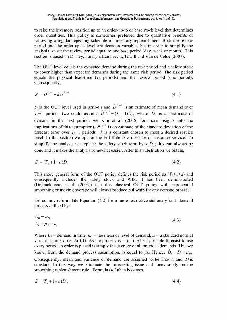
to raise the inventory position up to an order-up-to or base stock level that determines order quantities. This policy is sometimes preferred due to qualitative benefits of following a regular repeating schedule of inventory replenishment. Both the review period and the order-up-to level are decision variables but in order to simplify the analysis we set the review period equal to one base period (day, week or month). This section is based on Disney, Farasyn, Lambrecht, Towill and Van de Velde (2007). The OUT level equals the expected demand during the risk period and a safety stock to cover higher than expected demands during the same risk period. The risk period equals the physical lead-time (Tp periods) and the review period (one period). Consequently,

11 .ˆ pp TTt kDS . (4.1)

St is the OUT level used in period t and 1ˆ pTD is an estimate of mean demand over

Tp+1 periods (we could assume tpT DTD p ˆ)1(ˆ 1 , where tD̂ is an estimate of

demand in the next period, see Kim et al. (2006) for more insights into the

implications of this assumption). 1ˆ pT is an estimate of the standard deviation of the forecast error over Tp+1 periods. k is a constant chosen to meet a desired service level. In this section we opt for the Fill Rate as a measure of customer service. To

simplify the analysis we replace the safety stock term by tDa ˆ. ; this can always be

done and it makes the analysis somewhat easier. After this substitution we obtain,

tpt DaTS ˆ)1( . (4.2)

This more general form of the OUT policy defines the risk period as (Tp+1+a) and consequently includes the safety stock and WIP. It has been demonstrated (Dejonckheere et al. (2003)) that this classical OUT policy with exponential smoothing or moving average will always produce bullwhip for any demand process. Let us now reformulate Equation (4.2) for a more restrictive stationary i.i.d. demand process defined by:

tDt

D

D

D

0 (4.3)

Where Dt = demand in time, μD = the mean or level of demand, εt = a standard normal variant at time t, i.e. N(0,1). As the process is i.i.d., the best possible forecast to use every period an order is placed is simply the average of all previous demands. This we

know, from the demand process assumption, is equal to μD. Hence, .ˆDt DD

Consequently, mean and variance of demand are assumed to be known and D is constant. In this way we eliminate the forecasting issue and focus solely on the smoothing replenishment rule. Formula (4.2)then becomes,

DaTS p )1( . (4.4)


The remainder of Section 4.1 will focus on the replenishment as described by Equation (4.4). What happens now if we apply the above replenishment rule? The answer to that question is simple and known to most inventory managers (see for example Dejonckheere et al. (2003)). The OUT policy will generate replenishment orders that are the same as the last period’s observed demand. We simply order what the demand was in the current period (similar to a Just-In-Time strategy). That is why this policy is also called; “passing-on-orders” or “lot-for-lot” or even sometimes “continuous replenishment” when the length of the planning period has been shortened. Either way, the variability of the replenishment orders is exactly the same as the variability of the original demand. We will now turn the Order-Up-To policy into a smoothing rule. Recall it is defined as follows,

tt SO inventory position (4.5)

where tO is the ordering decision made at the end of period t. The inventory position

equals the net stock (NS) plus the “inventory on order but not yet arrived” (Work In Progress or WIP). The net stock equals inventory at hand minus backlog.

inventory position

forecast terminventory discrepancy term WIP discrepency term

1

. .

S

t p t t

t p t

O a T D NS WIP

D a D NS T D WIP

(4.6)

where Da. can be viewed as a target net stock (safety stock) and DTp . is a target

pipeline stock (on order inventory). We also need the inventory balance equation. It is

tTttt DONSNSp 11 . (4.7)

Expression (4.6) is the same as expression (4.5), but we decomposed the original formula into three components; a demand forecast, a net stock discrepancy term and a WIP or pipeline discrepancy term (see Dejonckheere et al. 2003). Moreover, if we now want to generate smooth replenishment patterns we can give an appropriate weight to the discrepancies as follows,

).().( tptt WIPDTNSDaDO . (4.8)

We now have two parameters, and , that will enable us to alter the dynamic behaviour of the supply chain. and are known to control engineers as proportional controllers or feedback gains. Proportional controllers are the simplest and most common controller in control systems. Indeed the very first control system, the Maxwell Governor, exploits a proportional controller in its velocity feedback loop (Åström, 2005). Proportional controllers can be thought of as simple amplifiers or


attenuators. In physical control systems they often take the form of electronic circuits or mechanical/pneumatic devices. In our application here they will most probably take the form of computer logic; and are constant multipliers of their respective feedback error. When 1 bullwhip is created (variance amplification) and for

1 a smoothed replenishment pattern is created (dampening). The optimal values of the two controllers are obviously sensitive to the economics of the supply chain in question.

This last issue concerning the economics of the supply chain brings us to the motivation of the policy proposed in (4.8). Expression (4.8) is able to generate a whole set of ordering patterns ranging from dampening (smoothing) to order variance amplification (bullwhip). The literature shows that production smoothing is efficient when firms face increasing marginal costs of production or the presence of production smoothing costs. A smoothing policy is efficient as long as the savings from not adjusting production exceeds the cost of holding extra inventory. We therefore propose in the next section two key performance measures; one to measure order variance amplification/dampening and the other to measure inventory variance amplification/dampening. In this way we hope to offer the reader a general framework. We are aware that this approach deviates from the standard approach in inventory theory where an optimal or near optimal policy will be derived given a set of inventory related costs. 4.2. Analysis of the smoothing rule under stationary demand The smoothing rule under stationary demand and matched controllers is equivalent to the well known exponential smoothing formula as it is given by

)( 11 tttt ODOO or ttt DOO .)1( 1 . (4.9)

If 1 expression (4.9) reduces to tt DO . This is equivalent to the traditional

OUT policy. Expanding Equation (4.9) results in:

ntn

tttt ODDDO )1(....)1()1(. 22

1 (4.10)

(4.9) and (4.10) tell us that the Order-Up-To policy reduces to exponential smoothing on replenishment orders. It also shows that the order quantity equals a convex combination of previous demand realizations. Balakrishnan et al. (2004) propose a general linear order smoothing policy of the following form,

0kktkt DO . (4.11)

Our smoothing policy is clearly a special case of the above general smoothing rule. More specifically, we propose an exponential smoothing scheme for the smoothing coefficients, k . It is easy to see that (4.9) will automatically yield less upstream

variance than the traditional Order-Up-To policy.


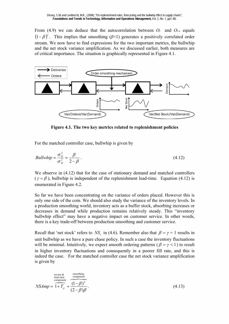
From (4.9) we can deduce that the autocorrelation between Ot and Ot-x equals

x1 . This implies that smoothing (β<1) generates a positively correlated order stream. We now have to find expressions for the two important metrics, the bullwhip and the net stock variance amplification. As we discussed earlier, both measures are of critical importance. The situation is graphically represented in Figure 4.1.

Figure 4.1. The two key metrics related to replenishment policies For the matched controller case, bullwhip is given by

22

2

D

OBullwhip . (4.12)

We observe in (4.12) that for the case of stationary demand and matched controllers ( ), bullwhip is independent of the replenishment lead-time. Equation (4.12) is enumerated in Figure 4.2. So far we have been concentrating on the variance of orders placed. However this is only one side of the coin. We should also study the variance of the inventory levels. In a production smoothing world, inventory acts as a buffer stock, absorbing increases or decreases in demand while production remains relatively steady. This “inventory bullwhip effect” may have a negative impact on customer service. In other words, there is a key trade-off between production smoothing and customer service. Recall that ‘net stock’ refers to tNS in (4.6). Remember also that = 1 results in

unit bullwhip as we have a pure chase policy. In such a case the inventory fluctuations will be minimal. Intuitively, we expect smooth ordering patterns ( 1 ) to result in higher inventory fluctuations and consequently in a poorer fill rate, and this is indeed the case. For the matched controller case the net stock variance amplification is given by

componentsmoothing

2component

time-lead & review

)2(

)1(1

pTNSAmp . (4.13)


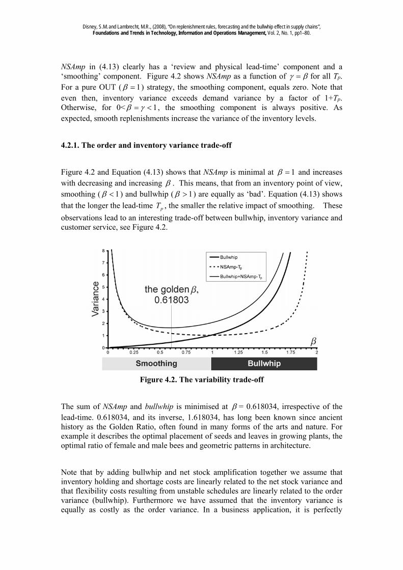
NSAmp in (4.13) clearly has a ‘review and physical lead-time’ component and a ‘smoothing’ component. Figure 4.2 shows NSAmp as a function of for all Tp. For a pure OUT ( 1 ) strategy, the smoothing component, equals zero. Note that even then, inventory variance exceeds demand variance by a factor of 1+Tp. Otherwise, for 0< 1 , the smoothing component is always positive. As expected, smooth replenishments increase the variance of the inventory levels.

4.2.1. The order and inventory variance trade-off

Figure 4.2 and Equation (4.13) shows that NSAmp is minimal at 1 and increases with decreasing and increasing . This means, that from an inventory point of view, smoothing ( 1 ) and bullwhip ( 1 ) are equally as ‘bad’. Equation (4.13) shows

that the longer the lead-time pT , the smaller the relative impact of smoothing. These

observations lead to an interesting trade-off between bullwhip, inventory variance and customer service, see Figure 4.2.

Figure 4.2. The variability trade-off

The sum of NSAmp and bullwhip is minimised at = 0.618034, irrespective of the lead-time. 0.618034, and its inverse, 1.618034, has long been known since ancient history as the Golden Ratio, often found in many forms of the arts and nature. For example it describes the optimal placement of seeds and leaves in growing plants, the optimal ratio of female and male bees and geometric patterns in architecture.

Note that by adding bullwhip and net stock amplification together we assume that inventory holding and shortage costs are linearly related to the net stock variance and that flexibility costs resulting from unstable schedules are linearly related to the order variance (bullwhip). Furthermore we have assumed that the inventory variance is equally as costly as the order variance. In a business application, it is perfectly


possible that the bullwhip effect and net stock amplification are not equally important and that costs are not related to the variance. Indeed, as we have mentioned before this is not the case when we have piecewise linear and convex inventory holding and backlog and piecewise linear and convex overtime and lost capacity costs (see section 2.3 and 6.5). Another interesting reference is Bertrand (1986) where a cost model was used to select appropriate values for the smoothing parameter. The production system he analysed is different from our model, but the paper offers an excellent example of how our metrics can be linked to a cost model.

4.2.2. The impact of bullwhip avoidance on customer service: The fill rate

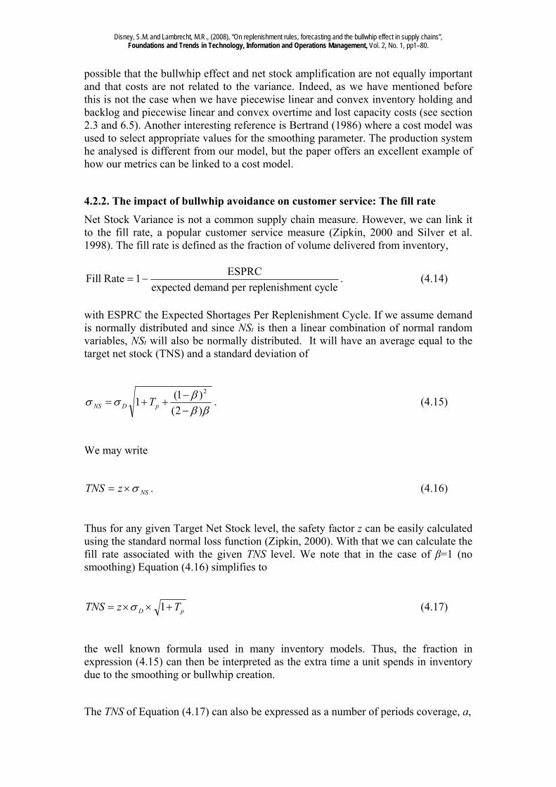
Net Stock Variance is not a common supply chain measure. However, we can link it to the fill rate, a popular customer service measure (Zipkin, 2000 and Silver et al. 1998). The fill rate is defined as the fraction of volume delivered from inventory,

ESPRCFill Rate 1

expected demand per replenishment cycle . (4.14)

with ESPRC the Expected Shortages Per Replenishment Cycle. If we assume demand is normally distributed and since NSt is then a linear combination of normal random variables, NSt will also be normally distributed. It will have an average equal to the target net stock (TNS) and a standard deviation of

)2(

)1(1

2

pDNS T . (4.15)

We may write

NSzTNS . (4.16)

Thus for any given Target Net Stock level, the safety factor z can be easily calculated using the standard normal loss function (Zipkin, 2000). With that we can calculate the fill rate associated with the given TNS level. We note that in the case of β=1 (no smoothing) Equation (4.16) simplifies to

pD TzTNS 1 (4.17)

the well known formula used in many inventory models. Thus, the fraction in expression (4.15) can then be interpreted as the extra time a unit spends in inventory due to the smoothing or bullwhip creation.

The TNS of Equation (4.17) can also be expressed as a number of periods coverage, a,


DaTNS . (4.18)

While the safety factor z is related to NS , a represents how many periods of average

demand D are covered by the TNS. The resulting ‘smoothing’ replenishment rule, guaranteeing a specified fill rate then equals Ot = D + ((Tp+a) D – NSt– WIPt). (4.19)

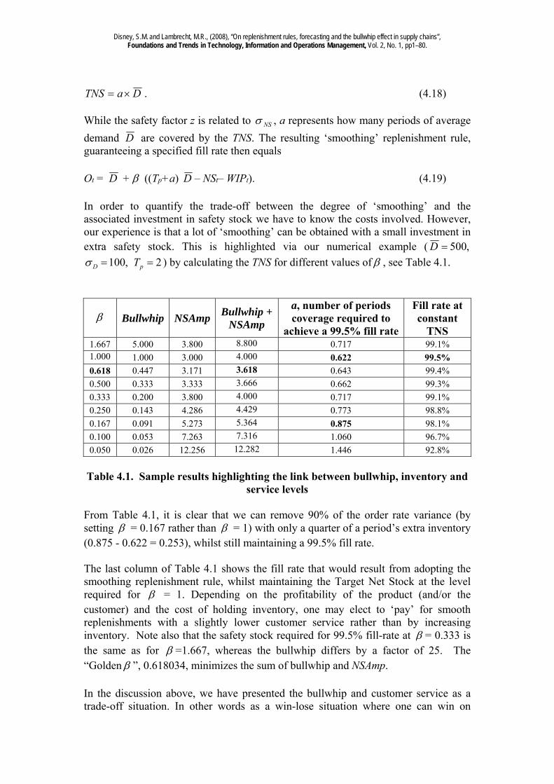
In order to quantify the trade-off between the degree of ‘smoothing’ and the associated investment in safety stock we have to know the costs involved. However, our experience is that a lot of ‘smoothing’ can be obtained with a small investment in extra safety stock. This is highlighted via our numerical example ( ,500D

,100D 2pT ) by calculating the TNS for different values of , see Table 4.1.

Bullwhip NSAmp Bullwhip +

NSAmp

a, number of periods coverage required to

achieve a 99.5% fill rate

Fill rate at constant

TNS 1.667 5.000 3.800 8.800 0.717 99.1% 1.000 1.000 3.000 4.000 0.622 99.5%

0.618 0.447 3.171 3.618 0.643 99.4%

0.500 0.333 3.333 3.666 0.662 99.3%

0.333 0.200 3.800 4.000 0.717 99.1%

0.250 0.143 4.286 4.429 0.773 98.8%

0.167 0.091 5.273 5.364 0.875 98.1%

0.100 0.053 7.263 7.316 1.060 96.7%

0.050 0.026 12.256 12.282 1.446 92.8%

Table 4.1. Sample results highlighting the link between bullwhip, inventory and

service levels From Table 4.1, it is clear that we can remove 90% of the order rate variance (by setting = 0.167 rather than = 1) with only a quarter of a period’s extra inventory (0.875 - 0.622 = 0.253), whilst still maintaining a 99.5% fill rate. The last column of Table 4.1 shows the fill rate that would result from adopting the smoothing replenishment rule, whilst maintaining the Target Net Stock at the level required for = 1. Depending on the profitability of the product (and/or the customer) and the cost of holding inventory, one may elect to ‘pay’ for smooth replenishments with a slightly lower customer service rather than by increasing inventory. Note also that the safety stock required for 99.5% fill-rate at = 0.333 is the same as for =1.667, whereas the bullwhip differs by a factor of 25. The “Golden ”, 0.618034, minimizes the sum of bullwhip and NSAmp. In the discussion above, we have presented the bullwhip and customer service as a trade-off situation. In other words as a win-lose situation where one can win on


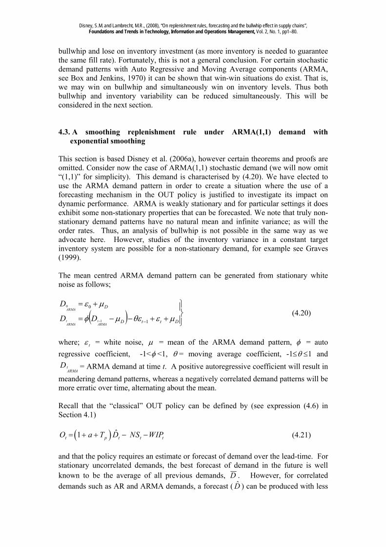
bullwhip and lose on inventory investment (as more inventory is needed to guarantee the same fill rate). Fortunately, this is not a general conclusion. For certain stochastic demand patterns with Auto Regressive and Moving Average components (ARMA, see Box and Jenkins, 1970) it can be shown that win-win situations do exist. That is, we may win on bullwhip and simultaneously win on inventory levels. Thus both bullwhip and inventory variability can be reduced simultaneously. This will be considered in the next section. 4.3. A smoothing replenishment rule under ARMA(1,1) demand with

exponential smoothing This section is based Disney et al. (2006a), however certain theorems and proofs are omitted. Consider now the case of ARMA(1,1) stochastic demand (we will now omit “(1,1)” for simplicity). This demand is characterised by (4.20). We have elected to use the ARMA demand pattern in order to create a situation where the use of a forecasting mechanism in the OUT policy is justified to investigate its impact on dynamic performance. ARMA is weakly stationary and for particular settings it does exhibit some non-stationary properties that can be forecasted. We note that truly non-stationary demand patterns have no natural mean and infinite variance; as will the order rates. Thus, an analysis of bullwhip is not possible in the same way as we advocate here. However, studies of the inventory variance in a constant target inventory system are possible for a non-stationary demand, for example see Graves (1999). The mean centred ARMA demand pattern can be generated from stationary white noise as follows;

DttD

D

tARMA

tARMA

ARMA

DD

D

1

0

1

0

(4.20)

where; t = white noise, = mean of the ARMA demand pattern, = auto

regressive coefficient, -1< <1, = moving average coefficient, -1 1 and

tARMA

D = ARMA demand at time t. A positive autoregressive coefficient will result in

meandering demand patterns, whereas a negatively correlated demand patterns will be more erratic over time, alternating about the mean. Recall that the “classical” OUT policy can be defined by (see expression (4.6) in Section 4.1)

ˆ1t p t t tO a T D NS WIP (4.21)

and that the policy requires an estimate or forecast of demand over the lead-time. For stationary uncorrelated demands, the best forecast of demand in the future is well known to be the average of all previous demands, D . However, for correlated demands such as AR and ARMA demands, a forecast ( D̂ ) can be produced with less


forecast error than D by using a forecasting mechanism such as exponential smoothing, Muth (1960). This is defined in (4.22) where Ta is the average age of the demand data in the forecast. Ta>-0.5 ensures a stable response, as the range

( 0.5, ]aT corresponds to (0,2] as 1

1 aT

so,

1 1

1ˆ ˆ ˆ1t t t t

a

D D D DT

= 11

ˆˆ ttt DDD . (4.22)

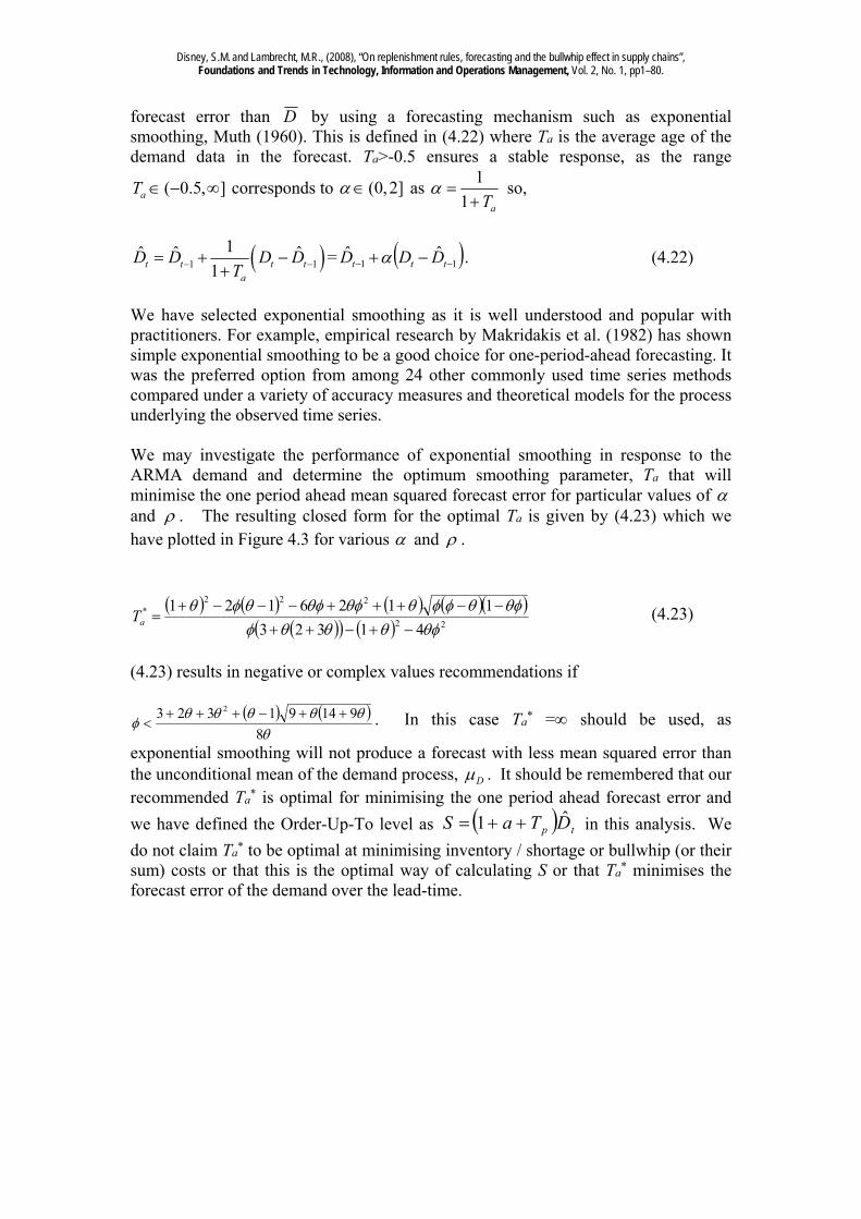
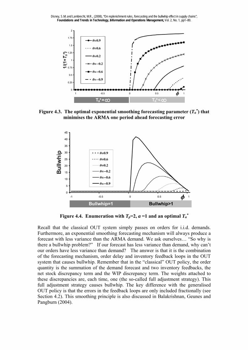
We have selected exponential smoothing as it is well understood and popular with practitioners. For example, empirical research by Makridakis et al. (1982) has shown simple exponential smoothing to be a good choice for one-period-ahead forecasting. It was the preferred option from among 24 other commonly used time series methods compared under a variety of accuracy measures and theoretical models for the process underlying the observed time series. We may investigate the performance of exponential smoothing in response to the ARMA demand and determine the optimum smoothing parameter, Ta that will minimise the one period ahead mean squared forecast error for particular values of and . The resulting closed form for the optimal Ta is given by (4.23) which we have plotted in Figure 4.3 for various and .

22

222*

41323

1126121

aT (4.23)

(4.23) results in negative or complex values recommendations if

8

91491323 2 . In this case Ta

* = should be used, as

exponential smoothing will not produce a forecast with less mean squared error than the unconditional mean of the demand process, D . It should be remembered that our recommended Ta

* is optimal for minimising the one period ahead forecast error and

we have defined the Order-Up-To level as tp DTaS ˆ1 in this analysis. We

do not claim Ta* to be optimal at minimising inventory / shortage or bullwhip (or their

sum) costs or that this is the optimal way of calculating S or that Ta* minimises the

forecast error of the demand over the lead-time.


Figure 4.3. The optimal exponential smoothing forecasting parameter (Ta*) that

minimises the ARMA one period ahead forecasting error

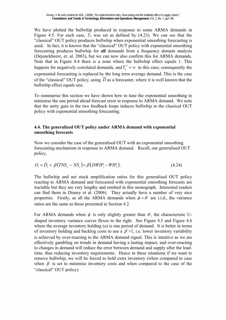
Figure 4.4. Enumeration with Tp=2, a =1 and an optimal Ta*

Recall that the classical OUT system simply passes on orders for i.i.d. demands. Furthermore, an exponential smoothing forecasting mechanism will always produce a forecast with less variance than the ARMA demand. We ask ourselves… “So why is there a bullwhip problem?” If our forecast has less variance than demand, why can’t our orders have less variance than demand? The answer is that it is the combination of the forecasting mechanism, order delay and inventory feedback loops in the OUT system that causes bullwhip. Remember that in the “classical” OUT policy, the order quantity is the summation of the demand forecast and two inventory feedbacks, the net stock discrepancy term and the WIP discrepancy term. The weights attached to these discrepancies are, each time, one (the so-called full adjustment strategy). This full adjustment strategy causes bullwhip. The key difference with the generalised OUT policy is that the errors in the feedback loops are only included fractionally (see Section 4.2). This smoothing principle is also discussed in Balakrishnan, Geunes and Pangburn (2004).


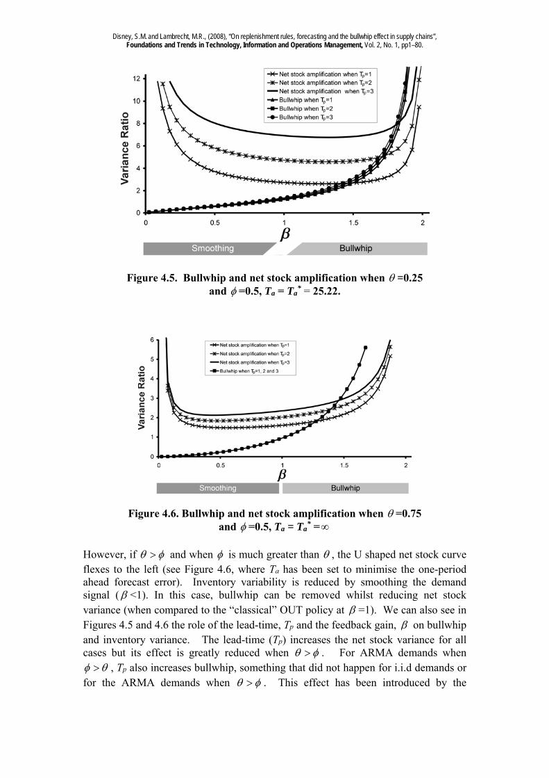
We have plotted the bullwhip produced in response to some ARMA demands in Figure 4.5. For each case, Ta was set as defined by (4.23). We can see that the “classical” OUT policy produces bullwhip when exponential smoothing forecasting is used. In fact, it is known that the “classical” OUT policy with exponential smoothing forecasting produces bullwhip for all demands from a frequency domain analysis (Dejonckheere, et. al. 2003), but we can now also confirm this for ARMA demands. Note that in Figure 4.4 there is a zone where the bullwhip effect equals 1. This happens for negatively correlated demands, and *

aT in this case; consequently the

exponential forecasting is replaced by the long term average demand. This is the case of the “classical” OUT policy, using D as a forecaster, where it is well known that the bullwhip effect equals one. To summarise this section we have shown how to tune the exponential smoothing to minimise the one period ahead forecast error in response to ARMA demand. We note that the unity gain in the two feedback loops induces bullwhip in the classical OUT policy with exponential smoothing forecasting. 4.4. The generalized OUT policy under ARMA demand with exponential smoothing forecasts Now we consider the case of the generalised OUT with an exponential smoothing forecasting mechanism in response to ARMA demand. Recall, our generalised OUT policy,

tttttt WIPDWIPNSTNSDO ˆ . (4.24)

The bullwhip and net stock amplification ratios for this generalised OUT policy reacting to ARMA demand and forecasted with exponential smoothing forecasts are tractable but they are very lengthy and omitted in this monograph. Interested readers can find them in Disney et al. (2006). They actually have a number of very nice properties. Firstly, as all the ARMA demands when are i.i.d., the variance ratios are the same as those presented in Section 4.2. For ARMA demands when is only slightly greater than , the characteristic U-shaped inventory variance curves flexes to the right. See Figure 4.5 and Figure 4.6 where the average inventory holding (a) is one period of demand. It is better in terms of inventory holding and backlog costs to use a >1, i.e. lower inventory variability is achieved by over-reacting to the ARMA demand signal. This is intuitive as we are effectively gambling on trends in demand having a lasting impact, and over-reacting to changes in demand will reduce the error between demand and supply after the lead-time, thus reducing inventory requirements. Hence in these situations if we want to remove bullwhip, we will be forced to hold extra inventory (when compared to case when is set to minimise inventory costs and when compared to the case of the “classical” OUT policy).


Figure 4.5. Bullwhip and net stock amplification when =0.25 and =0.5, Ta = Ta

* = 25.22.

Figure 4.6. Bullwhip and net stock amplification when =0.75 and =0.5, Ta = Ta

* =

However, if and when is much greater than , the U shaped net stock curve flexes to the left (see Figure 4.6, where Ta has been set to minimise the one-period ahead forecast error). Inventory variability is reduced by smoothing the demand signal ( <1). In this case, bullwhip can be removed whilst reducing net stock variance (when compared to the “classical” OUT policy at =1). We can also see in Figures 4.5 and 4.6 the role of the lead-time, Tp and the feedback gain, on bullwhip and inventory variance. The lead-time (Tp) increases the net stock variance for all cases but its effect is greatly reduced when . For ARMA demands when

, Tp also increases bullwhip, something that did not happen for i.i.d demands or for the ARMA demands when . This effect has been introduced by the


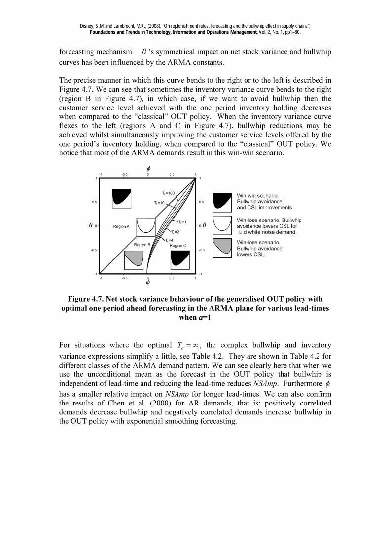
forecasting mechanism. ’s symmetrical impact on net stock variance and bullwhip curves has been influenced by the ARMA constants. The precise manner in which this curve bends to the right or to the left is described in Figure 4.7. We can see that sometimes the inventory variance curve bends to the right (region B in Figure 4.7), in which case, if we want to avoid bullwhip then the customer service level achieved with the one period inventory holding decreases when compared to the “classical” OUT policy. When the inventory variance curve flexes to the left (regions A and C in Figure 4.7), bullwhip reductions may be achieved whilst simultaneously improving the customer service levels offered by the one period’s inventory holding, when compared to the “classical” OUT policy. We notice that most of the ARMA demands result in this win-win scenario.

Figure 4.7. Net stock variance behaviour of the generalised OUT policy with optimal one period ahead forecasting in the ARMA plane for various lead-times

when a=1

For situations where the optimal aT , the complex bullwhip and inventory

variance expressions simplify a little, see Table 4.2. They are shown in Table 4.2 for different classes of the ARMA demand pattern. We can see clearly here that when we use the unconditional mean as the forecast in the OUT policy that bullwhip is independent of lead-time and reducing the lead-time reduces NSAmp. Furthermore has a smaller relative impact on NSAmp for longer lead-times. We can also confirm the results of Chen et al. (2000) for AR demands, that is; positively correlated demands decrease bullwhip and negatively correlated demands increase bullwhip in the OUT policy with exponential smoothing forecasting.


Demand Pattern

Bullwhip NSAmp

AR(1) 2

1(2 ) 1 1

2 2

2 1 2 1 1 1

1 1 21 1 1

pTp p p

T T T

MA(1) 2

1 2 2

(2 ) 1

2

2 2

1 2 1 2 2

2 1pT

ARMA (1,1)

2

2

1 2 1 1

(2 ) 1 1 1 2

2

22

2 2

1 1 2

2 2

2 1 1

11 1

1 1 2 1 1 1 2

pT

pT

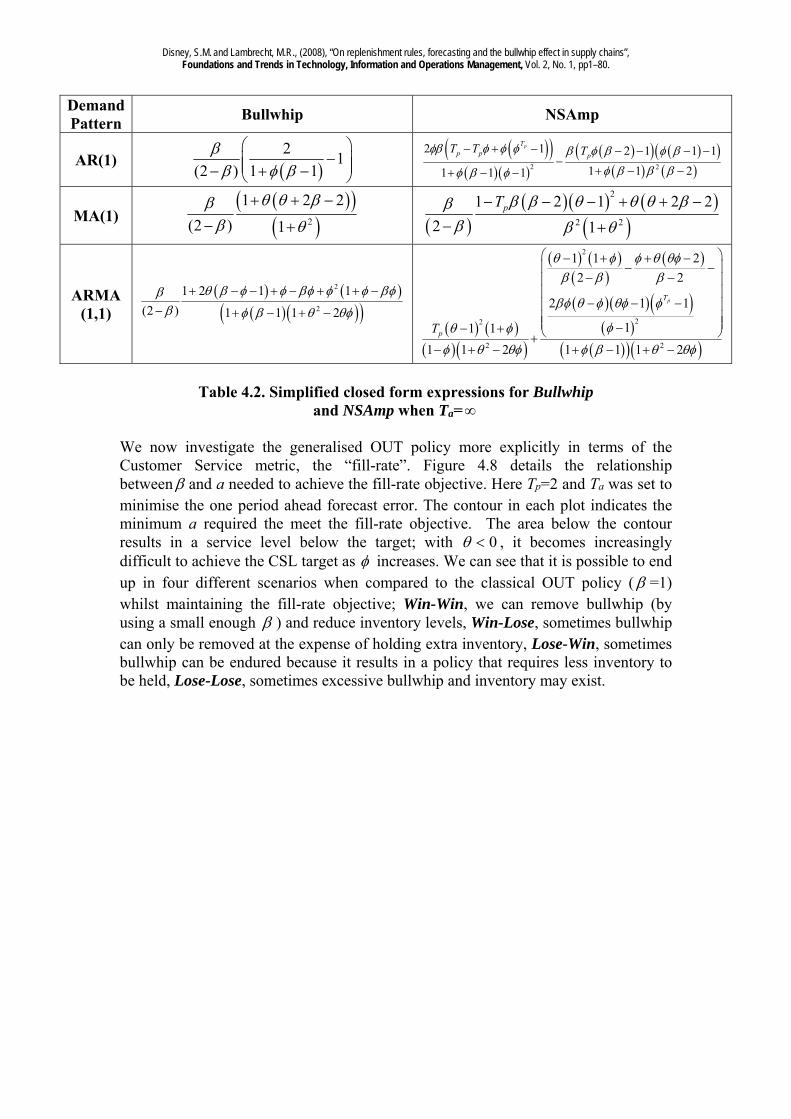
Table 4.2. Simplified closed form expressions for Bullwhip

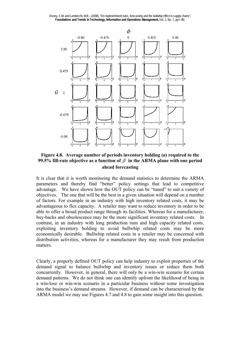
and NSAmp when Ta= We now investigate the generalised OUT policy more explicitly in terms of the Customer Service metric, the “fill-rate”. Figure 4.8 details the relationship between and a needed to achieve the fill-rate objective. Here Tp=2 and Ta was set to minimise the one period ahead forecast error. The contour in each plot indicates the minimum a required the meet the fill-rate objective. The area below the contour results in a service level below the target; with 0 , it becomes increasingly difficult to achieve the CSL target as increases. We can see that it is possible to end up in four different scenarios when compared to the classical OUT policy ( =1) whilst maintaining the fill-rate objective; Win-Win, we can remove bullwhip (by using a small enough ) and reduce inventory levels, Win-Lose, sometimes bullwhip can only be removed at the expense of holding extra inventory, Lose-Win, sometimes bullwhip can be endured because it results in a policy that requires less inventory to be held, Lose-Lose, sometimes excessive bullwhip and inventory may exist.


Figure 4.8. Average number of periods inventory holding (a) required to the 99.5% fill-rate objective as a function of in the ARMA plane with one period

ahead forecasting It is clear that it is worth monitoring the demand statistics to determine the ARMA parameters and thereby find “better” policy settings that lead to competitive advantage. We have shown how the OUT policy can be “tuned” to suit a variety of objectives. The one that will be the best in a given situation will depend on a number of factors. For example in an industry with high inventory related costs, it may be advantageous to flex capacity. A retailer may want to reduce inventory in order to be able to offer a broad product range through its facilities. Whereas for a manufacturer, buy-backs and obsolescence may be the more significant inventory related costs. In contrast, in an industry with long production runs and high capacity related costs, exploiting inventory holding to avoid bullwhip related costs may be more economically desirable. Bullwhip related costs in a retailer may be concerned with distribution activities, whereas for a manufacturer they may result from production matters.

Clearly, a properly defined OUT policy can help industry to exploit properties of the demand signal to balance bullwhip and inventory issues or reduce them both concurrently. However, in general, there will only be a win-win scenario for certain demand patterns. We do not think one can identify upfront the likelihood of being in a win-lose or win-win scenario in a particular business without some investigation into the business’s demand streams. However, if demand can be characterised by the ARMA model we may use Figures 4.7 and 4.8 to gain some insight into this question.


4.5. Minimum mean squared error forecasting

We continue to study the role of forecasting in relation to the bullwhip effect and net stock amplification. In the previous section we studied ARMA demand patterns with the exponential forecasting method. In this section we study a forecasting procedure that minimizes the mean squared error for an AR(1) underlying demand process. We assume that the demand can be described by an AR(1) model,

tDtDt DD 1 , (4.25)

where Dt is the demand during period t, μD is a constant mean of the demand, εt is an i.i.d. normally distributed random error and is the first-order autocorrelation

coefficient with 1 .

For the above demand process, the Minimum Mean Squared Error (MMSE) forecasting is applied to predict the lead time demand. Recall, Tp is the lead-time. With this forecasting technique, the demand forecast is derived in such a way that the forecast error is minimized. The MMSE forecast for the demand in period t + τ equals the conditional expectation of Dt+τ, given current and previous demand observations Dt, Dt-1, Dt-2,… Box and Jenkins (1970). Doing so, we exploit the underlying nature of the demand pattern to predict future demand. As a consequence it seems logical to explicitly forecast the τ-period-ahead demand to predict lead time demand, instead of simply multiplying the one-period-ahead forecast with the lead time (as in the MA

and ES forecasting technique). Let ,...,, τD τt 21ˆ , be the τ-period-ahead forecast of

demand Dt+τ made in period t. Then,

DtDt DD 1ˆ (4.26)

and

Dtτ

Dτt DD ˆ . (4.27)

The lead time demand forecast is obtained by plugging the τ-period-ahead forecast

into the definition of lead time demand,

1

1

1 ˆˆ pp T

i itTt DD . Hence, in contrast to the

moving average and exponential smoothing forecast methods, we do not multiply the one-period ahead forecast with the lead time, but instead calculate the forecast of the demand over the lead time horizon and review period, 1pT . The MMSE forecast

for lead time demand is then given by

Dt

T

DpTt D

ρ

ρρTD

p

p

11ˆ

21 . (4.28)

Clearly, the MMSE forecasting scheme is optimal at minimising the variance of the forecast error of future demands, as it explicitly takes the correlated demand structure into account. This is not the case in the non-optimal moving average and exponential


smoothing procedures. When demand is i.i.d. ( =0), the above equations reveal that the MMSE forecast reduces to a constant equal to the mean demand. It is interesting to observe the closed form expressions for our two metrics,

Bullwhip = )1(

)1)(1(21

21

pp TT

(4.29)

and

NSAmp =

2

212

)1(

)2)(1()1(1

pp TT

pT. (4.30)

These results hold if the MMSE forecasting scheme is used in a classical Order-Up-To policy. Zhang (2004) showed that the MMSE forecasting method is clearly the winner among the three forecasting methods of moving average, exponential smoothing and MMSE, if only inventory costs are considered at a single echelon. That is, it leads to the lowest inventory cost when the cost function in Equation (2.3) is used. Moreover, it can be shown (Zhang (2004), Alwan et al. (2003), Hosoda (2005)) that there is no bullwhip effect for a negatively correlated process under an optimal MMSE forecasting scheme. In other words, for negatively correlated demand, the variability in orders is dampened with respect to the observed demand. This is a very important result and it demonstrates how important the interplay is between forecasting methods, demand processes and replenishment rules. This is the main conclusion of Section 4. 5. Transferring the inventory decisions to the upstream levels: Vendor

Managed Inventory as a variance reduction tool In a traditional supply chain, each level in the supply chain issues production/replenishment orders without considering the situation at either up- or downstream tiers of the supply chain. There is no formal collaboration, no information sharing and no collaborative forecasting procedures. Consequently most players in supply chains do not respond directly to the market but respond to replenishment orders from downstream echelons. This creates distorted demand information in the supply chain and consequently the bullwhip effect. In the previous sections we focused on new replenishment rules to dampen variability, in this section we propose to shift the inventory decision rights from the downstream to the upstream member of the supply chain. The latter approach is better known as Vendor Managed Inventories (VMI). Under VMI, downstream players share demand and inventory position information with the upstream players who then make inventory replenishment decisions (Lee and Chu, 2005). One may even go one step further and let the supplier not only to make stock level decisions, but also to own the goods until they are sold or assembled in a product (sometimes this is called consignment stocking). VMI contracts often stipulate restrictions such as the right to return excess stock to the upstream or in case of a consignment stock agreement the right to charge


inventory carrying costs if the inventory flow time exceeds a certain agreed upon time limit. Although VMI has been extensively covered in the literature, many suppliers have little incentive to accept the process. The arguments being that an investment in IT technology is required, the inventory-carrying cost and warehousing costs are shifted to the supplier, lowering once again the thin profit margins. Thus, there is a need to develop a theory on the “economics of VMI”. Let’s therefore enumerate the most important advantages of VMI. First VMI eliminates one decision point and merges the replenishment decision with the production and materials planning of the supplier. Here, the supplier takes charge of the customer’s inventory replenishment on the operational level, and uses this visibility in planning his own supply operations, e.g. more efficient production schedules and transportation planning. With VMI, multi-echelon supply chains then can act in a coordinated way. There is no need to design supply chain contracts and upstream suppliers can choose a reorder quantity that best fits the production system. VMI often results in more frequent replenishments and consequently the order quantity variance is reduced. Economies in transportation can also be obtained through route planning and optimization of truck fill and with other methods such as joint replenishment and inventory routing techniques. The VMI model is, in other words, a channel coordination strategy between downstream and upstream players. VMI allows the supplier to proactively plan his production and shipments to the customer, instead of reacting to the customer’s orders and thus may yeild some production and transportation economies. Additionally, the supplier often has a much better market knowledge about his products than the retailer. Therefore, he is in a better position to generate forecasts and this leads to improved inventory performance and customer service levels at every stage of the supply chain. VMI may also result in a tighter retailer-supplier relationship and thus can be considered a buy-in strategy. We briefly illustrate the benefits of VMI with a real life example, Boute and Lambrecht (2007). We analyze the ordering pattern of a bakery company focusing on authentic specialties in the biscuit and cake world: caramelized biscuits, waffles, frangipane, and cake specialties amongst others. For certain products, a make-to-order policy is employed and the assumptions used in this paper are largely satisfied. In 2002, the firm introduced a VMI program implemented in the SAP software. In Figure 5.1 we show a graph of the shipments from the production facility to the distribution centre of a retailer (for one specific product) in the pre-VMI period (2001-mid 2002) and the shipments in the post-VMI implementation period (mid 2002-2005). The coefficient of variation of the shipment quantities went down from 1.14 to 0.45 (a number observed for other products as well). We were also able to collect (post-VMI) data on the shipments from the distribution centre of the retailer to the different retail outlets. For the specific product discussed above, we obtain a coefficient of variation of 0.40.


Figure 5.1. The impact of VMI on the order variability The company now benefits from a higher flexibility in its production planning, since the VMI program allows the company to plan proactively instead of reactively. It is also able to utilize the production facilities more efficiently, as the outputs need not be ramped up and down based on large swings in orders. It reduced its transportation costs considerably due to an improved and more stable transport planning. Moreover, inventories decreased both at the manufacturer and at the retailer, improving the freshness of the products of the end consumer. Finally, the customer service level improved as product availability increased, thereby increasing the profitability for both the manufacture and the retailer. 6. Coordination of replenishment rules in a multi-echelon setting In this section we study a two-echelon supply chain model consisting of a retailer and a manufacturer reacting to stationary i.i.d. stochastic consumer demand. It is based upon Disney et al. (2008). Both echelons implement our periodic review generalized Order-Up-To policy (OUT) replenishment policy with matched controllers. Consequently both echelons incur costs that we assume to be directly proportional to the long term variance of the inventory level and the long term variance of the replenishment orders. The combined total cost of the retailer and manufacturer has to be minimized. This can be done in several ways. One possibility is that both the retailer and the manufacturer act independently and minimize their own local costs. However, another possibility is that the retailer and manufacturer coordinate their replenishment decisions to reach a globally optimal solution. This supply chain coordination is not only realized through sharing demand information, but the actors also have to share information with respect to the parameters of the replenishment rules used and their lead-times. This is of course a far more advanced coordination scheme than what is often proposed in the literature.


Assume demand is a stationary i.i.d. random process with a positive mean, DD 4 , greater than four standard deviations of the demand variance to ensure the likelihood of negative demand is negligible. Under this assumption the best possible forecast for

all future demands (to minimise the mean squared error) is Dt DD ˆ . That is, to

set the forecast tD̂ , to a time invariant constant D , equal to the unconditional mean

of the demand process, D . To recap, the generalised OUT policy with matched controllers is given by

11

ˆ ˆ ˆ.p

t

T

t t t t p t ti

WIP

O D aD NS T D O

(6.1)

When the demand forecast is set equal to the mean of the demand process then this reduces to

11

( . )pT

t t p ti

O D aD NS T D O

. (6.2)

After substitution and simplifcation (see Disney et al., (2006a)) we obtain

1 1( )t t t tO O D O . (6.3)

6.1. The retailer’s order and inventory variance Let us now start to construct our two echelon supply chain model by first considering the retailer. The retailer’s demand from the consumers is a stationary i.i.d. random process. Later we will assume the retailer incurs two types of costs; one directly proportional to the long-run variance of the retailers inventory level and the other directly proportional to the long-run variance of the retailer replenishment orders placed on the supplier (manufacturer). So we wish to quantify these variances produced by the retailer’s replenishment rule. This has already been presented earlier in Section 4.2.1 but we will present here again.

2

2 2RO

D

(6.4)

In Equation (6.4) 2

D denotes the variance of consumer demand and 2RO is the

variance of orders placed by the retailer on the manufacturer. Interestingly we note that under the assumptions of; stationary i.i.d demand, forecasts generated by conditional expectation, and matched feedback controllers, bullwhip is independent of the lead-time, Tp. If either of these assumptions is not meet, than the bullwhip effect does depend upon the lead-time, Tp. The variance of the retailer’s net stock is (inventory on hand minus backlog) given by


2 2

2

(1 )1

(2 )RNS

pD

T

. (6.5)

2RNS denotes the variance of the retailers net stock. When Tp=1 (a further assumption

we will make later in order to ease the exposition of our investigation on the manufacturer in the supply chain) Equation (6.5) reduces to

2, 1

2

2 1

2pRNS T

D

. (6.6)

For completeness we note that the variance of WIP is given by Equation (6.7), which is of the same form as the smoothing component in the inventory variance equation.

2 2

2

( 1)

2WIP

D

(6.7)

6.2. The manufacturer’s order and inventory variance The manufacturer responds to the retailer’s orders and we assume that he uses our generalised OUT policy with matched controller, Equation (6.1), for scheduling production. For simplicity, we assume, from this point on for the rest of this section unless explicitly stated, a unit replenishment lead-time at both the retailer and the manufacturer exists. It is remarkable to note that the retailer’s lead-time does not influence the order variances at either echelon of the supply chain. In fact, the retailer’s lead-time only affects the retailer’s inventory levels, whilst the manufacturer’s lead-time influences both the manufacturer’s order and inventory variance. The retailers order process, after passing through the generalised OUT policy, is now auto-correlated. Thus, we may exploit this structural information to forecast both the demand over the lead-time and the demand in the period after the lead-time with conditional expectation. This alters the way in which the target pipeline content

( tDTp ˆ. in (6.1)) and the target net stock ( tDa ˆ in (6.1)) is calculated in the generalised

OUT policy, but has the advantage of generating optimal forecasts. These forecasts are optimal in the sense that they minimise the mean squared error between the forecast and its realisation over the lead-time and review period. The manufacturers order variance for the case when Tp=Mp=1 is given by

2 22

2

2 2 2

2 1 2

M M MMO

D M M M

(6.8)

and the manufacturer’s inventory variance when Tp=Mp=1 is given by


222

2

2 2

2

M MMNS

D M M

(6.9)

where, is the retailer’s proportional feedback controller, as before, and M is the

corresponding feedback controller in the manufacturer’s replenishment policy. More details about how these variance ratios where obtained can be found in the Disney et al. (2008). The limit values of (6.8) and (6.9) contain some interesting insights. When approaches zero, the manufacturers order and inventory variances both go to zero. This is due to the fact that the retail orders are simply a constant (equal to the mean demand). When the manufacturers feedback gain, M , approaches zero, the variance

of the manufacturers net stock is infinite. This is because the net stock is now an accumulation of random variables and is non-stationary with no natural mean. Equation (6.9) shows that decreasing will reduce the manufacturer’s inventory

requirements, but decreasing M will increase the manufacturer’s inventory

requirements. In the following sections, we develop several supply chain policies ranging from local optimization to global optimization. 6.3. The sequential optimisation scenario: The self-serving focus In order to test various supply chain policies, we have to define a cost function to be used. We will first assume that the costs in the supply chain are linearly related to the variance of the order rate and inventory levels at each echelon in the supply chain. For example, we assume the inventory holding and shortage costs are linearly related to the inventory variance, and production / replenishment on-costs resulting from variable schedules are linearly related to the order variance. Furthermore we assume inventory variance is equally as costly as order variance. Later in section 6.5 we will consider the case when costs are linearly related to the standard deviations. These two cost functions (variances and standard deviations) may of course be subject to debate. The 2 2 and RNS MNS terms are linked to the safety stock needed (see Disney

et al. (2008)) and consequently cover inventory holding costs of the safety stock and backorder costs. The 22 and MORO terms are linked to production switching costs or

adjustments costs due to order rate changes (capacity adjustment costs). We also consider order rate variance (standard deviation in section 6.3) as equally important as inventory level variance (standard deviation in section 6.3). It is however perfectly possible that the bullwhip may be more costly then inventory variance amplification or vice versa, depending on the context. In this case we have to apply weights to these factors. This may change the shape of the cost curves that are derived in this paper. We refer to Disney, Towill and Van de Velde (2004), for an investigation on such weighting schemes. Alternative objective cost functions are also discussed in Kim and Ryan (2003), Disney and Grubbström (2004) and Chen and Disney (2007).


6.3.1. The selfish retailer First, let us consider the retailer. If the retailer only incurs inventory related costs (that is, the costs related to the order variance are constant or zero) then the retailer costs are given by (6.6) and the optimal behaviour of the retailer is to set =1 as minimising (6.6) w.r.t. results in *=1. However if the retailer has both inventory and order related costs then his costs are given by (6.10),

2 2

£ 2 2

1 2

2RO RNS

D D

R

(6.10)

and the optimum 5 1

0.6180342

, the golden ratio, as we saw earlier in

Section 4.2. 6.3.2. The selfish manufacturer Now let us consider the manufacturer. If the retailer has used =1 to minimise the retailers inventory costs, the manufacturer faces a demand pattern that is exactly equal to the consumers demand as the retailer has simply “passed on the orders”. The manufacturer’s variance ratio and cost analysis in this case is exactly the same as the retailer’s variance trade-off. Thus our previous remarks in Section 6.3.1 for the retailer hold for the manufacturer (after the obvious change in notation). That is the manufacturer’s cost and the optimal feedback controller, *

M , are given by (6.10) and

the golden ratio respectively. However, if the retailer has used the golden in the inventory and WIP feedback loops, then the manufacturer’s demand process has changed, and thus, his actions now have different consequences. Let us illustrate further. Using (6.8) and (6.9), with equal to the golden ratio, the manufacturer’s order and inventory variance (and their sum) is shown in Figure 6.1.


Figure 6.1. The manufacturer’s variance trade-off with a golden retailer

Figure 6.1 shows there is a much greater region of order smoothing in the manufacturers replenishment policy with a golden retailer as the manufacturers order variance is less than unity for all M >1.06471. The manufacturer’s local cost when

both inventory and order variance costs are present is given by

£

90 5 200 541 241 5 284 126 5 29 13 5

2 5 3 5 2 2 5 5

M M M

M M M

M

.

(6.11) Differentiating (6.11) w.r.t. M , solving for zero gradient and selecting the relevant

root yields

*

,M O NS

=0.589296 (6.12)

However, if the manufacturer’s cost function consists of costs associated with the variance of the inventory levels only, then the cost function to be minimised is

£

5 3 5 5 3 2 2

4 2

M M

M M

M

. (6.13)

Again minimising (6.13) w.r.t M yields,

*

,M O NS

=1. (6.14)


Summarising our results from the sequential local optimisation of the supply chain we have developed the following table that details the feedback gains and the resulting costs.

Manufacturer incurs

Inventory variance costs only

Inventory and order variance costs

Ret

aile

r in

curs

Inve

nto

ry

vari

ance

co

sts

only

* = 1 *M = 1

R£ = 2 M£ = 2 SC£ = 4

* = 1 *M = 0.61803

R£= 2 M£ = 2.61803 SC£ = 4.61803

Inve

nto

ry

and

ord

er

vari

ance

co

sts

* = 0.61803 *M = 1

R£ = 2.61803 M£ = 1.11146 SC£ = 3.72946

* = 0.61803 *M = 0.589296

R£ = 2.61803 M£ = 1.661384 SC£ = 4.299418

Table 6.1. The self-serving solutions

6.4. The global optimisation problem: Supply chain coordination In this section we will show that the self-serving focus results in poor performance by considering what happens when supply chain members coordinate the replenishment decisions. Equations (6.4), (6.5), (6.8) and (6.9) allow us to explore the complete solution space for feedback design in our supply chain. More specifically, we can compute the values of the feedback controllers that the supply chain parties can use to improve overall costs. For example, the following contour plots (Figure 6.2) illustrate the performance of the supply chain for all possible settings.


Manufacturer incurs

Inventory variance costs only Inventory and order variance

costs R

etai

ler

incu

rs

Inve

nto

ry v

aria

nce

cos

ts o

nly

Inve

nto

ry a

nd

ord

er

vari

ance

cost

s

Figure 6.2. The complete supply chain total cost solution space with costs related to the variance of order rates and inventory levels

Using numerical techniques we have been able to find the actual optimal settings for

* and *M to minimise global supply chain costs as shown in Table 6.2.

Manufacturer incurs



Ret

aile

r in

curs

Inve

nto

ry

vari

ance

co

sts

only

* = 0.437097 *M = 1

R£ = 2.46828 M£ = 0.657735 SC£ = 3.12156

* = 0.381329 *M = 0.568085

R£ = 2.6201 M£ = 0.939129 SC£ = 3.55922

Inve

nto

ry

and

ord

er

vari

ance

co

sts

* = 0.390526 *M = 1

R£ = 2.833627 M£ = 0.547575 SC£ = 3.3812

* = 0.347278 *M = 0.565464

R£ =2 .951647 M£ = 0.829541 SC£ = 3.78119

Table 6.2. The global optimum supply chain solutions


By comparing the £SC in Table 6.1 and 6.2, we observe that supply chain gains are

realized by a global optimization (for all scenarios). The coordinating mechanism dominates the non-coordinating mechanism. The supply chain gain, however, is allocated to the manufacturer and the retailer incurs higher costs. This of course will not result in a coordination policy. Cachon (2003) describes what is needed to coordinate the supply chain: “if a coordinating contract can allocate rents arbitrarily, then there always exists a contract that Pareto dominates a non-coordinating contract, i.e. each firm’s profit is no worse off and at least one firm is strictly better off with the coordinating contract”. Therefore part of the supply chain gain has to be allocated to the retailer so that the retailer has an economic incentive to cooperate. For all scenarios the gain is large enough to compensate the cost increase of the retailer. That means that the cost of the retailer, after allocation, is not worse and the manufacturer is strictly better off with coordination. In the global solution, is larger than in the local optimization solution. Consequently the retailer will incur a larger variance of the inventory level which results in a higher level of safety stock to guarantee a given level of customer service. The extra investment in safety stock has to be compensated by the supply chain gain in order to motivate the retailer to participate. This can be realized by a lower price charged by the manufacturer. In Table 6.3 we quantify a naïve solution of = M =1 to benchmark a practice quite

often found in industry. In this case the members of the supply chain are interested in minimizing investment in inventory and consequently follow a naïve JIT strategy. We can see that the naïve solution (that is not accommodating for the supply chain cost structures and failing to tune replenishment rules accordingly) is always more costly than the case where supply chain players act rationally and minimize their local costs. Superior performance occurs when supply chain players “think outside the box” and act to minimize global supply chain costs.

=1

M =1

Manufacturer incurs Inventory variance costs

only Inventory and order variance

costs

Ret

aile

r in

curs

Inve

nto

ry

vari

ance

co

sts

only

R£ = 2 M£ = 2 SC£ = 4

R£ = 2 M£ = 3 SC£ = 5

Inve

nto

ry

and

ord

er

vari

ance

co

sts R£ = 3

M£ = 2 SC£ = 5

R£ = 3 M£ = 3 SC£ = 6

Table 6.3. The naïve solution


6.4.2. The altruistic retailer

As indicated by Cachon (2003), supply chain members may consider coordination mechanisms (and the corresponding contracts) costly and complicated. Our global optimization policy requires that (i) forecasts are generated with conditional expectation, (ii) a proportional OUT policy is employed throughout the supply chain (iii) that the feedback controllers are globally optimized. This may be hard to implement. We therefore suggest in this section an “easier to implement” policy. We will compare the results of this strategy with the three previous policies (the local optimum solution, the global optimum solution and the naïve solution). We assume that the manufacturer is following a low inventory policy and sets 1M .

The retailer however, is willing and able to alter his replenishment rule to incorporate a proportional controller in the feedback rule. We call this policy the “altruistic retailer” policy. The results are shown in Table 6.4. As can be seen from Table 6.4, the altruistic retailer can obtain near optimal performance for the supply chain by a proper reaction (i.e., by tuning the feedback controllers of the replenishment rule) to the non-cooperative manufacturer. In fact the performance is within 5% of the true optimum when the manufacturer has both inventory and order variance costs; there is no difference in the costs if the manufacturer has only inventory variance costs.

M =1 Manufacturer incurs



Ret

aile

r in

curs

Inve

nto

ry

vari

ance

co

sts

only

= 2.28782 R£ = 2.46828

M£ = 0.657735 SC£ = 3.12156

= 2.87386 R£ = 2.739587 M£ = 0.990137 SC£ = 3.72972

Inve

nto

ry

and

ord

er

vari

ance

co

sts

= 2.56065 R£ = 2.833627 M£ = 0.547575 SC£ = 3.3812

= 3.09894 R£ = 3.039953 M£ = 0.890773 SC£ = 3.930725

Table 6.4. The altruistic retailer

6.5. Linking the variance ratios to costs in the supply chain In this section we will quickly explore an alternative cost function based on a more traditional, OR / inventory theory approach. Some costs may be assumed to be constant or independent of the inventory levels or orders, but we simply ignore them here. Such costs may be materials, energy and administration overheads, for example. However to capture the costs that may reasonably be assumed to be dependent on the inventory levels and order rates we will assume a linear system with normally


distributed demand exists with piece-wise linear, convex inventory holding costs then the holding costs are

Holding costs =

otherwise 0

0 if tt NSNSH, (6.15)

where H is a the unit cost of holding a unit in inventory per period. Likewise if piece-wise linear, convex backlog costs exist,

Backlog costs =

otherwise 0

0 if )( tt NSNSB, (6.16)

where B is the cost of a backlog per unit per period, and we set the safety stock target

* 12NS

H Bk erf

H B

(6.17)

to achieve the economic stock-out probability, then the inventory related costs will be given by (Disney et al. (2006b)),

2

1

$min

Holding Backlog costs2

H Berf

H BNS B H e

I

. (6.18)

We notice from (6.18) that the inventory holding and backlog costs are linearly related to the standard deviation of the net stock levels. k* can be related back to our

approach we used earlier to set the TNS via the relation D

ka

*

.

In a similar manner, if there are piece-wise linear, convex lost capacity costs of

Lost capacity costs =

otherwise 0

if DSOODSN tt , (6.19)

where S is the slack capacity above the mean demand rate (not to be confused with the traditional variable associated with the OUT level) and N is the cost per unit per period of not producing to the available production capacity and there are piece-wise linear, convex over-time costs of

Overtime costs =

otherwise 0

if DSODSOP tt , (6.20)

where P is the cost per unit per period of producing in over-time, and we invest in enough capacity (above / below average demand) to achieve an economic over-time probability,


* 12O

N PS erf

N P

, (6.21)

then the bullwhip related costs are equal to (Disney et al. (2006b),

2

1

$min

Lost capacity Over-time costs2

N Perf

N PO N P e

C

. (6.22)

Equation (6.22) shows us that the bullwhip costs are linearly related to the standard deviation of the order rates. Thus, it is interesting to investigate an objective function where the standard deviations, rather than the variances, of the inventory levels and order rates are used as building blocks. For ease of exposition, we will restrict ourselves here to the case where the standard deviations of the inventory levels and order rates are equally weighted; that is when H=N and B=P (or interestingly when H=P and B=N) at both echelons. This change to the objective function has a number of implications, but we note that major conclusions we have drawn so-far remain qualitatively unchanged. Consider first the local optimisation collaboration scheme, the self serving solutions outlined in Section 6.3. The objective function for the retailer when only inventory costs are present becomes

£

1

2RNS pR T

, (6.23)

and the feedback gain that minimises the retailers cost is =1. This is the same result as before when we considered the variance of the inventory levels and it implies that the manufacturer faces i.i.d. demand when the retailer considers only his inventory cost are important. However, when the retailer has costs related to the standard deviation of both inventory levels and order rates the objective function becomes

£

1

2 2RO RNSR Tp

. (6.24)

Minimising (6.24) w.r.t. results in the following expression for *

1/3 1/32/3 2/3

*2/3 2/3 1/32/3

2/3

2 1 2 1 2 411 1 2

2 2 11

p p p

p pp

p

T T T

T T T

T

.

(6.25)


We notice that the golden ratio solution no longer exists and the optimal * is now dependent on the retailers lead-time, Tp. Analytical analysis of the manufacturers standard deviation costs is rather lengthy, and thus we resort to a numerical investigations for the case of Tp=Mp=1. The solution space is portrayed graphically is very similar to Figure 4; enough so, that our major conclusions (altruistic behaviour on behalf of the retailer with either a smart or naïve manufacturer, improves overall supply chain performance) remain unchanged, although absolute numbers are slightly different. Table 6.5, details the four specific supply chain cooperation strategies for the different cost structures. Again, the internal relationships and its relationship to the self-serving solutions remain intact.

Manufacturer incursInventory standard deviation costs only

Inventory and order standard deviation costs

Naive Local Altruistic Global Naive Local Altruistic Global

Ret

aile

r in

curs

Inve

nto

ry

stan

dar

d

dev

iati

on

cost

s on

ly 1 1 0.282367 0.282367 1 1 0.181132 0.198942

M 1 1 1 1 1 0.435421 1 0.553122

R£ 1.41421 1.41421 1.74981 1.74981 1.41421 1.41421 2.00881 2.27938

M£ 1.41421 1.41421 0.561212 0.56121 2.41421 2.09849 0.859025 0.86359

SC£ 2.82843 2.82843 2.31102 2.31102 3.82843 3.51271 2.86783 2.8162

Inve

nto

ry

and

ord

er

stan

dar

d

dev

iati

on

cost

s

1 0.435421 0.217316 0.217316 1 0.435421 0.153642 0.163839

M 1 1 1 1 1 0.471807 1 0.575123

R£ 2.41421 2.09849 2.24157 2.24157 2.41421 2.09849 2.4157 2.37816

M£ 1.41421 0.80851 0.44196 0.44196 2.41421 1.45936 0.75344 0.74684

SC£ 3.82843 2.907 2.68577 2.68577 4.82843 3.55786 3.16914 3.125

Table 6.5. The supply chain solutions when costs are linearly related to the

standard deviation To summarise all of our investigations considered in this section, we have standardised (by defining the naïve designs costs as 100%) all of the costs in the different supply chain collaboration schemes with both the variance and standard deviation versions of our objective function. These are shown in Table 6.6. Again we highlight that the head-line results are similar for both cost functions (variance or standard deviations).

For the naïve strategy, players in the supply only need to operate with standard replenishment software and have a standard trading relationship with their customers and suppliers. It is an easy option. But the naïve strategy results in an inefficient use of inventory and capacity. So to improve their performance, players should make re-engineering efforts to minimise lead-times and additionally create the most accurate forecasts they can achieve. These changes will directly improve business performance. Indeed, these efforts are required for all supply chains and will reduce inventory requirements in supply chains.


More perceptive players will try to understand their own cost structures, demand patterns and tune their replenishment rules in order to minimise their own local costs. This may be an appropriate strategy if a player has a very large customer or supply base, is geographically or culturally separated or is unwilling or unable to collaborate with others. In order to be tune the OUT policy in the manner we have investigated here, some adjustments to computer code or decision support systems may be required. For example a grocery retailer we have worked with has actually re-coded their in-house, bespoke replenishment system to incorporate a proportional controller in the WIP and inventory feedback loops. Other companies we have worked with who have standard ERP software have exploited spreadsheet based decision support systems to assist replenishment analysts when they conduct final conformation of replenishment decisions.

Manufacturer incurs

Inventory costs only Inventory and order costs

Ret

aile

r in

curs

Inve

nto

ry c

osts

on

ly

Supply chain design

Variance costs

Standard deviation

costs

Supply chain design

Variance costs

Standard deviation

costs Naïve 100 100 Naïve 100 100

Self serving 100 100 Self serving 92.36 91.75 Altruistic 78.04 81.71 Altruistic 74.59 74.91 Globally optimal 78.04 81.71 Globally

optimal 71.18 73.56

Inve

nto

ry a

nd

or

der

cos

ts

Supply chain design

Variance costs

Standard deviation

costs

Supply chain design

Variance costs

Standard deviation

costs Naïve 100 100 Naïve 100 100

Self serving 74.59 75.93 Self serving 71.66 73.69 Altruistic 67.62 70.15 Altruistic 65.51 65.63 Globally optimal 67.62 70.15 Globally

optimal 63.02 64.72

Table 6.6. Standardised cost summary

6.6. Practical considerations The global optimisation strategy requires players to first intimately understand their own business, as well as other players cost structures, demand patterns and replenishment rules and to be able to tune their replenishment rules appropriately. Furthermore, some agreement has to be reached to re-allocate the supply chain “gains” between the players. This should be possible as the global optimisation strategy Pareto dominates the self serving solution. However in a supply chain with an extended vendor base, it may be difficult to gain the commitment from the large number of suppliers and the re-engineering effort will increase substantially. The altruistic retailer strategy, although not as efficient as the global optimal strategy has good performance with considerably less effort as there are no supply chain re-


engineering requirements essential to the manufacturer. It only requires the retailer to understand cost structures, demand rates, lead-times and replenishment rules throughout the supply chain. It may also not even be necessary to have a formal re-allocation of the supply chain gain. This could be redistributed though traditional pricing polices and the willingness of manufacturers to accept cost reductions over time. Other attractions may also exist for the retailer to behave altruistically. For example, the UK grocery company who has reduced the bullwhip produced by their replenishment rules (via incorporating a proportional controller discussed therein) did so in order to reduce the workload variability in their warehouse and transportation activities. Furthermore, from a queuing theory viewpoint, bullwhip reduction may actually have a compensating effect on inventory requirements due to reduced manufacturing lead-times, Boute et al. (2007). This may help to offset the predicted extra inventory investment at the retailer. This will be especially important for retailers concerned about maintaining a wide product range with correspondingly large requirements for shelf space. 6.7. Summary Four different cost scenarios were constructed using the variance expressions and four different optimisation strategies where undertaken; a naïve solution, a local optimum solution, an altruistic retailer solution, and a global optimum solution. The naïve solution resulted in the worst performance. Interestingly, when total supply chain costs are considered, the classic OUT policy is not optimal in a multi-echelon scenario, even when only inventory costs exist. We demonstrated this with three different optimisation strategies. The first of these was a local optimisation strategy where the retailer first tuned his replenishment rule to minimise his costs and the manufacturer then tuned his replenishment rule accordingly. This improved the performance of the supply chain from a global perspective, but was not globally optimal. This global optimal was identified from our variance ratios numerically and plotted graphically. Inspection of these results, lead us to the final scenario where action as only taken by the retailer. Although this scenario is not optimal, reasonable performance from the supply chain could be achieved from the altruistic retailer, without re-engineering efforts at the manufacturer. In order to achieve this coordination scheme, supply chain players need to share information about demand patterns, replenishment policies, parameter settings and lead-times. We concede that this may be difficult to achieve. However, our experience suggests that both retailers and manufacturers may have other incentives over and above the supply chain gains we have discussed here to undertake such seemingly altruistic behaviour.

It is interesting to note that in this simple two-echelon supply chain model, the best result comes from the players acting in the best interest of the supply chain, and not by the players acting solely in their own immediate interest. This is in contrast to Adam Smith, for example, who argued that the best result for a group resulted from


each individual player acting solely in own interests. It is however congruent with the arguments of John Nash. Superior performance is achievable if firms coordinate their actions. 7. New directions in bullwhip research We now briefly review a small number of research streams we are currently working on in our quest to solve the bullwhip problem. 7.1. The square root law for bullwhip Let’s turn our focus now to a distribution network. Assume that we have multiple retailers being served by a number of distribution centres. All transportation lead-times are the unity, regardless of the number of distribution centres that exist. Each retailer faces i.i.d. demand with the same mean and variance. Furthermore each retailer and distribution centre employs a traditional OUT policy with MMSE forecasting and unit feedback gains. For such a scenario Maister (1976) introduced the “Square Root Law for Inventory” when consolidation occurs in the distribution network. Quoting directly from Maister,

“If the inventories of a single product (or stock keeping unit) are originally maintained at a number (n) of field locations (refereed to as the decentralised system) but are then

consolidated into one central inventory then the ratio ninventory system dcentralise

inventory system seddecentrali exists,

Maister (1976)” Amazingly, the square root law also exists for bullwhip costs. Consider the capacity related costs at the DC echelon. Equation (7.1) shows us that bullwhip or capacity costs are given by

YC O£ ;

2

21 2

1

PN

Nerf

ePNY . (7.1)

Y is a constant determined by the lost capacity and overtime costs. This was derived in Section 6.5. It is easy too prove the square root law for bullwhip exists by considering that in the decentralised supply chain the standard deviation of the orders

at each of the n distribution centres is 2cO , and in the centralised supply chain

(with only one distribution centre) the standard deviation of the orders is 2cO n .

Thus,

n

Yn

Yn

c

c 2

2

costs bullwhip dcentralise

costs bullwhip seddecentrali

, (7.2)

which is the “Square Root Law for Bullwhip”, Disney, McCullen and Saw (2006). This result surprised us, as intuitively, we expected it to have the opposite impact. This result also suggests that reasons to consolidate distribution networks are actually a lot stronger than previously thought (as this is often based solely on inventory


costs). The likely impact of this is to force companies to consolidate even further than they have in the past, increasing the amount of traffic on the road. Thus, internalising the external costs transportation causes is now even more important. Extending this approach to consider more complex demand processes, arbitrary lead times, sophisticated forecasting techniques and novel replenishment rules seem to be a very profitable research area. 7.2. Multi-product scenarios Joint replenishment polices (JRP) which control more than one product in the same inventory replenishment decision is a very promising but complex issue. It is closely related to the inventory routing problem (IRP) and there are some initial results on both the JRP and the IRP that have some interesting properties and show improved economic performance, Mustaffa and Disney (2005). This is especially true when order set-up or transportation costs are considered. Another variation of the multi-product scenario is the case where the demand for one product influences the demand for another product. This type of interaction could be captured by the so-called Vector Auto Regressive (VAR) demand process, Sadeghi and Disney (2007). 7.3. Stochastic lead-times Recently we have discovered that there is a link between smoothing and lead-times. We have been using queuing theory to model a manufacturer. The manufacturer works on a make-to-order, first come, first served basis. When a retailer smoothes his replenishment order that is placed on a manufacturer, the lead-time that the manufacturer needs to produce and deliver the products is reduced. Thus, there is a link between bullwhip and lead-time variability Boute et al. (2007). The smoother the retailer’s order is, the quicker the manufacturer can replenish his order, on the average. Thus, there is actually a mechanism to break the bullwhip, inventory trade-off we spoke of in Section 4.2.1. Other research that has also recently considered similar problems; Chatfield et al. (2004) has investigated the impact of stochastic lead-times, information quality and information sharing in the OUT policy via a simulation experiment. This approach is further clarified with analytical insights in Kim et al. (2006). 7.4. Multi-echelon supply chain scenarios When we consider multi-echelon supply chains there are a whole range of new options available to us. For example, we have already spoke of VMI, here downstream supply chain states are communicated to suppliers and this information is used in their replenishment decisions. This type of arrangement is closely related to what is known as the echelon-stock policy or the echelon order-up-to policy, Hoberg et al. (2007). Collaboration and coordination mechanisms for multi-echelon supply chains also have very good economic performance as we have discussed in Section 6. For example, if a retailer is willing and able to smooth his replenishment orders he places on his supplier, the supplier will be able to manufacture product more efficiently. However, this is effectively an altruistic contribution on behalf of the retailer if the supplier does not share the gains with the retailer, Hosoda and Disney (2006). There is a lot more research to conduct on this type of collaboration.


Interestingly, there may also be a benefit to mis-specification of the demand process. For example, if an AR(p) demand process is forecasted with a non-optimal forecasting technique such as exponential smoothing and capacity and inventory costs exist then superior performance can sometimes result in a single or multi-echelon setting. In a multi-echelon case it is even possible to deliberately mis-specify the demand process, forecast this mis-specified demand with conditional expectation and gain an economic benefit. It appears that optimal forecasts are only cost optimal in supply chains for single echelon scenarios where only inventory cost exist, Hosoda and Disney (2007). Finally, there is a novel method discussed in Gaalman and Disney (2007b) for co-ordinating a multi-echelon supply chain. This policy has been derived using optimal control theory and, in a sense, is like a VMI supply chain in reverse. The core of the idea is that because the retailer’s lead-time is shorter than the manufacturer’s lead-time, he can correct some of the manufacturer’s forecast errors. In this way, the retailer is accounting for the state of the “upstream” supply chain. The analysis of this policy is not yet complete but initial findings are promising. In general multi-echelon policies offer a very promising route for future bullwhip analysis. However, they will require a significant industrial engineering effort to implement in practice. Collaboration and co-ordination mechanisms are also needed. However, the biggest problem with multi-echelon research is properly capturing the effect of lost sales and capacity constraints. This is very difficult to achieve as these systems are non-linear. However, Markov Chains do offer a means of analysis and will even cope with quantised systems where only integer amount of products can be ordered from a supplier or production system. 7.5. Concluding remarks Finally, if you would like to explore more about the bullwhip effect, please go to www.bullwhip.co.uk. There you will find a collection of simulations, java explorers, table top games and reference lists associated with the bullwhip effect. 8. References Alwan, L.C., Liu, J.J. and Yao Dong-Qing, (2003) “Stochastic characterization of

upstream demand processes in a supply chain”, IIE Transactions, 35, pp207-219. Asl, F.M. and Ulsoy, A.G., (2003) “Analysis of a system of linear delay differential

equations”, Journal of Dynamic Systems, Measurement and Control 125, pp215-222.

Åström, K.J., (2005), Control System Design, Preprint, http://www.cds.caltech.edu/ ~murray/courses/cds101/fa02/caltech/astrom.html, Verified 17th September 2005.

Aviv, Y. (2003) “A time-series framework for supply-chain inventory management”, Operations Research, 51 (2), pp210-227.

Balakrishnan, A., Geunes, J. and Pangburn, M., (2004) “Coordinating supply chains by controlling upstream variability propagation”, Manufacturing & Service Operations Management, 6 (2), pp163-183.


Bertrand, J.W.M., (1986) "Balancing production level variations and inventory variations in complex production systems", International Journal of Production Research, 24 (5), pp1059-1074.

Boute, R.N. and Lambrecht, M.R., (2007) “Altruistic behaviour in supply chain management”, Tijdschrift voor Economie en Management, Forthcoming.

Boute, R.N., Disney, S.M., Lambrecht, M. and Van Houdt, B., (2007), “An integrated production and inventory model to dampen upstream demand variability in the supply chain”, European Journal of Operational Research, 178 (1), pp121-142.

Box, G.E.P and Jenkins, G.M., (1970) Time series analysis forecasting and control. Holden-Day, San Francisco.

Buck, J.R. and Hill, T.W., (1971) "Laplace transforms for the economic analysis of deterministic problems in engineering", The Engineering Economist, 16 (4), pp247-263.

Butman, J., (2002) “A pain in the (supply) chain”, Harvard Business Review, 80 (5), pp31-44.

Cachon, G. and Fisher, M., (1997) “Campbell soup’s continuous product replenishment program: Evaluation and enhanced decision rules”, Production and Operations Management, 6, pp266-276.

Cachon, G., (2003) “Supply chain coordination with contracts” in de Kok, A. and S. Graves, Supply Chain Management: Design, Coordination and Operations, pp229-339.

Chatfield, D.C., Kim, J.G., Harrison, T.P. and Hayya, J.C. (2004) “The bullwhip effect ~ Impact of stochastic lead time, information quality, and information sharing: A simulation study”, Production and Operations Management, 13 (4), pp340-353.

Chen, F., Samroengraja, R., (2000) “The stationary beer game”, Production and Operations Management, 9 (1), pp19-30.

Chen, Y.F. and Disney, S.M., (2007) “The myopic order-up-to policy with a feedback controller”, International Journal of Production Research, 45 (2), pp351-368.

Chen, Y.F., Drezner, Z., Ryan J.K. and Simchi-Levi, D., (2000) “Quantifying the Bullwhip effect in a simple supply chain: The impact of forecasting, lead-times and information”, Management Science, 46, pp436-443.

Childerhouse, P., Aitken, J. and Towill, D.R., (2002) “Analysis and Design of Focused Demand Chains”, Journal of Operations Management, 20, pp675-689.

Christopher, M. and Towill, D.R., (2002) “Developing Market Specific Supply Chain Strategies”, International Journal of Logistics Management, 13 (1), pp1-14.

Corless R.M., (2004) “The Lambert W function”, http://www.cecm.sfu.ca/ publications/ organic/ rutgers/node34.html, Verified July 2004.

Corless, R.M., Gonnet, G.H., Hare, D.E.G., Jeffrey, D.J. and Knuth, D.E., (1996) “On the Lambert W function”, Advances in Computational Mathematics, 5, pp329-359.

Croson, R. and Donohue, K., (2002) “Experimental economics and supply-chain management”, Interfaces, 32 (5), pp74-82.

Croson, R., and Donohue, K., (2003) “Impact of POS data sharing on supply chain management: An experimental study,” Production and Operations Management, 12 (1), pp1-11.

Dejonckheere, J., Disney, S.M., Lambrecht, M.R. and Towill, D.R., (2004) “The impact of information enrichment on the bullwhip effect in supply chains: A control engineering perspective”, European Journal of Operational Research, 153 (3), pp727-750.


Dejonckheere, J., Disney, S.M., Lambrecht, M.R. and Towill, D.R., (2003) “Measuring and avoiding the bullwhip effect: A control theoretic approach”, European Journal of Operational Research, 147 (3), pp567-590.

Disney, S.M., (2001) The production and inventory control problem in Vendor Managed Inventory supply chains, PhD Thesis, Cardiff University, Wales.

Disney, S.M. and Grubbström, R.W., (2004) “The economic consequences of a production and inventory control policy”, International Journal of Production Research, 42 (17), pp3419-3431.

Disney, S.M. and Naim, M.M., (1999) “Improving the effectiveness of supply chains”, 15th International Conference on Production Research, Limerick, August, pp637-640.

Disney, S.M., Chen, Y.F., van de Velde, W., Warburton, R., Gaalman, G., Lambrecht, M. and Towill, D.R., (2006b) “Economics of the bullwhip effect”, Annual INFORMS International Conference, June 25-28, Hong Kong.

Disney, S.M., Farasyn, I., Lambrecht, M., Towill, D.R. and Van de Velde, W., (2006a) “Taming the bullwhip effect whilst watching customer service in a single echelon of a supply chain”, European Journal of Operational Research, 173, pp151-172.

Disney, S.M., Farasyn, I., Lambrecht, M.R., Towill, D.R. and Van de Velde, W., (2007) “Controlling bullwhip and inventory variability with the golden smoothing rule”, European Journal of Industrial Engineering, 1 (3), pp241-265.

Disney, S.M., Lambrecht, M., Towill, D.R. and Van de Velde, W., (2008) “The value of coordination in a two echelon supply chain: Sharing information, policies and parameters”, IIE Transactions, http://www.informaworld.com/smpp/title~content=t713772245~db=all~tab=issueslist~branches=40 - v4040 (3), pp341-355.

Disney, S.M., McCullen, P. and Saw, R.J., (2006) “Dynamic supply chain design: Square root law for bullwhip”, Proceedings of the International Symposium on Logistics, Beijing, China, 9th-12th July.

Disney, S.M., Naim, M.M. and Potter, A., (2004) “Assessing the impact of e-business on supply chain dynamics”, International Journal of Production Economics, 89 (2), pp109-118.

Disney, S.M., Towill, D.R. and Van de Velde, W., (2004) “Variance amplification and the golden ratio in production and inventory control”, International Journal of Production Economics, 90 (3), pp295-309.

Fliess, M., Marquez, R. and Mounier, H., (2002) “An Extension of Productive Control, PID Regulators and Smith Predictors to Some Linear Delay Systems”, International Journal of Control, 75, pp728-743.

Forrester, J., (1961), Industrial dynamics, MIT Press, Cambridge MA, USA. Gaalman, G. and Disney, S.M., (2006) “State space investigation of the bullwhip

problem with ARMA(1,1) demand processes”, International Journal of Production Economics, 104 (2), pp327-339.

Gaalman, G. and Disney, S.M., (2007a) “On Bullwhip in a Family of Order-up-to Policies with ARMA(2,2) Demand and Arbitrary Lead-Times”, Accepted for publication in the International Journal of Production Economics. http://dx.doi.org/10.1016/j.ijpe.2006.11.024.

Gaalman, G. and Disney, S.M., (2007b) “On the echelon-order-up-to policy: A stochastic optimal control approach”, Manufacturing and Service Operations Management Conference, Beijing, June 18-19.


Graves, S.C., (1999) “A single-item inventory model for a non-stationary demand process”, Manufacturing and Service Operations Management, 1 (1), pp50-61.

Grubbström, R.W., (1967) “On the application of the Laplace transform to certain economic problems”. Management Science, 13 (7), pp558-567.

Hammond, J.H., (1994) “Barilla SpA(A)”, Harvard Business School Case 6-694-046, Boston, MA.

Hoberg, K., Bradley, J.R. and Thonemann, U.W., (2007) “Analysing the effect of the inventory policy on order and inventory variability with linear control theory”, European Journal of Operational Research, 176 (3), pp1620-1642.

Holland, W., Sodhi, M.S., (2004) “Quantifying the effect of batch size and order errors on the bullwhip effect using simulation”, International Journal of Logistics Research and Applications, 7 (3), 251-261.

Holweg, H., Disney, S.M., Holmström, J. and Småros, J., (2005), “Supply chain collaboration: Making sense of the strategy continuum”, European Management Journal, 23 (2), pp170-181.

Hosoda, T. and Disney, S.M., (2007) “Mis-specification of demand in supply chains”, Working Paper, Cardiff Business School, Cardiff University, UK.

Hosoda, T. and Disney, S.M., (2006) “The governing dynamics of supply chains: The impact of altruistic behavior”, Automatica, 42, pp1301-1309.

Hosoda, T., (2005) “The principles governing the dynamics of supply chains”, PhD Thesis, Cardiff University, UK.

Hoyt, D., (2001) “Solectron: from contract manufacturer to global supply chain integrator”, Stanford University Graduate School of Business, Case GS-24, Stanford, CA.

IBM Business Consulting Services, (2005) “The specialized enterprise: A fundamental redesign of firms and industries”, 21 pp.

Jacobs, F.R., (2000) "Playing the beer distribution game over the internet", Production and Operations Management, 9 (1), pp31-39.

Jury, E.I., (1964) Theory and application of the z-transform method. Robert E. Krieger Publishing Company, New York.

Kalman, R.E., (1960) “A new approach to linear filtering and prediction problems”, Transactions of the ASME-Journal of Basic Engineering, 82, Series D, pp35-45.

Kim, H-K and Ryan, J.K., (2003) "The cost impact of using simple forecasting techniques in a supply chain", Navel Research Logistics, 50, pp388-411.

Kim, J.G., Chatfield, D.C., Harrison, T.P. and Hayya, J.C., (2006) “Quantifying the bullwhip effect in a supply chain with stochastic lead time”, European Journal of Operational Research, 173, pp617-636.

Konicki, S., (2002), “Now in bankruptcy, Kmart struggled with supply chain”, Information Week, http://www.informationweek.com/story/IWK20020125S0020 Verified on 28th January 2002.

Kuper, A. and Branvold, D., (2000) “Innovation diffusion at Hewlett Packard”, in M.E. Johnson and D.F. Pyke, eds. “Supply chain management: innovations for education”, Miami, FL., pp205-218

Lam, D.A. and Miron, J.A. (1996) “The effects of temperature on human fertility”, Demography, 33 (3), pp291-305.

Lee, C.C. and Chu, W.H.J. (2005), “Who should control inventory in a supply chain?”, European Journal of Operational Research, 164, pp158-172.

Lee, H.L., Padmanabhan, V. and Whang, S. (2004) “Comments on “Information distortion in a supply chain: The bullwhip effect” The bullwhip effect: A reflection”, Management Science, 50 (12), pp1887-1893.


Lee, H.L., Padmanabhan, V. and Whang, S., (1997a) “The bullwhip effect in supply chains”, Sloan Management Review, Spring, 38 (3), pp93-102.

Lee, H.L., Padmanabhan, V. and Whang, S., (1997b) “Information distortion in a supply chain: The bullwhip effect”, Management Science, 43 (4), pp546-558.

Looman, A., Ruttins, F.A.J. and de Boer, L., (2002) “Designing ordering and inventory management methodologies for purchased parts”, Journal of Supply Chain Management, 38 (12), pp22-29.

Machuca, J.A.D. and Barajas, R.P., (1997) “A computerized network version of the beer game via the Internet”, Systems Dynamic Review, 13 (4), 323-340.

Maister, D.H., (1976) “Centralisation of Inventories and the "Square Root Law"”, International Journal of Physical Distribution, 6 (3), pp124-134.

Makridakis, S., Andersen, A., Carbone, R., Fildes, R., Hibon, M., Lewandowski, R., Newton, J., Parzen, R., & Winkler, R., (1982) “The accuracy of extrapolation (time series) methods: Results of a forecasting competition”. Journal of Forecasting, 1, pp11-153.

Munson, C.L., Hu, J. and Rosenblatt, M., (2003) “Teaching the costs of uncoordinated supply chains”, Interfaces, 33 (3), 24-39

Mustaffa, N.H. and Disney, S.M., (2005) “Approaches to solving the inventory routing problem”, EUROMA International Conference on Operations and Global Competitiveness, Budapest, Hungary, 19th-22nd June, pp767-774.

Muth, J.F. (1960) “Optimal properties of exponentially weighted forecasts”. Journal of the American Statistical Association, 55, pp299-306.

Ortmeyer, G., Quelch, J. and Salmon, W., (1991) “Restoring credibility to retail pricing”, Sloan Management Review, Fall, pp55-66.

Ouyang, Y. and Daganzo, C. (2006) “Characterization of the bullwhip effect in linear, time-invariant supply chains: Some formulae and tests”, Management Science, 52 (10), pp1544-1556.

Peleg, B., (2003) “STMicroelectronics e-chain optimization project: Achieving streamlined operations through collaborative forecasting and inventory management”. Stanford Global Supply Chain Management Forum Case, Stanford University, Stanford, CA.

Potter, A. and Disney, S.M., (2006) “Bullwhip and batching: An exploration”, International Journal on Production Economics, 104 (2), pp408-418.

Sadeghi, A. and Disney, S.M., (2007) “Quantifying the bullwhip effect in a two product supply chain”, Working Paper, Cardiff Business School, Cardiff University, UK.

Silver, E.A., Pyke, D.F. and Peterson, R., (1998) Inventory management and production planning and scheduling. John Wiley and Sons, New York, USA.

Simchi-Levi, D., Kaminsky, P. and Simchi-Levi, E., (1998) Designing and managing the supply chain: Concepts, strategies and case studies, McGraw-Hill International Edition, 498 pp.

Simon, H., (1952) “On the application of servomechanism theory in the study of production control”, Econometrica, 20, pp247-268.

Smith, O.J., (1959) “A controller to overcome dead time”. Instrument Society of America – Journal, 6 (2), pp28–33.

Sterman, J.D. (1989) “Modelling managerial behaviour: Misperceptions of feedback in a dynamic decision making experiment”, Management Science, 35 (3), pp321-339.

Towill, D.R. (1994) "1961 and all that: the influence of Jay Forrester and Jack Burbidge on the design of modern manufacturing systems", Proceedings of the


1994 International Systems Dynamics Conference on Business Decision Making, Stirling, pp105-15.

Towill, D.R., Lambrecht, M.R., Disney, S.M. and Dejonckheere, J. (2003) “Explicit filters and supply chain design”, Journal of Purchasing and Supply Management, 9 (2), pp73-81.

Tsypkin Y.Z. (1958) “Theory of Pulse Systems”, (In Russian), State Press for Physics and Mathematical Literature, Moscow.

Tsypkin, Y.Z., (1964), Sampling systems theory and its application, Vol. 2, Pergamon Press, Oxford.

Tustin, A., (1947a) “A method of analysing the behaviour of linear systems in terms of time series”, Journal of the IEE, 94, Part IIA, pp130-142.

Tustin, A., (1947b) “The effects of backlash and of speed-dependent friction on the stability of closed-cycle control systems”, Journal of the IEE, 94, Part IIA, pp143-151.

Tustin, A., (1947c) “A method of analysing the effect of certain kinds of non-linearity in closed-cycle control systems”, Journal of the IEE, 94, Part IIA, pp152-160.

Tustin, A., (1947d) “The nature of the operator's response in manual control and its implementations for controller design”, Journal of the IEE, 94, Part IIA, pp190-202.

Van Horne, C. and Marier, P., (2007) “The Quebec wood supply game: An innovative tool for knowledge management and transfer”, available for download at http://forac.fsg.ulaval.ca/fileadmin/docs/Publications/QCWoodSupplyGame.pdf

Vassian H.J., (1955) “Application of discrete variable servo theory to inventory control”, Journal of the Operations Research Society of America, 3 (3), pp272-282.

Warburton, R.D.H. and Disney, S.M., (2007) “Order and inventory variance amplifications: The equivalence of discrete and continuous time analysis”, Accepted for publication in International Journal of Production Economics. http://dx.doi.org/10.1016/j.ijpe.2007.02.021

Zhang, X., (2004) “The impact of forecasting methods on the bullwhip effect”, International Journal Production Economics, 88, 15-27.

Zipkin, P.H., (2000) Foundations of inventory management, McGraw-Hill, New York, USA.

Date post:	23-Apr-2018
Category:	Documents
Upload:	doanliem
View:	230 times
Download:	2 times

On replenishment rules, forecasting and the bullwhip ... - On replenishment rules... · Disney,...

Documents