1 Accepted for publication in FLOW MEASUREMENT AND INSTRUMENTATION http://dx.doi.org/10.1016/j.flowmeasinst.2016.02.003 On sampling bias in multiphase flows: Particle image velocimetry in bubbly flows T. Ziegenhein*, D. Lucas Helmholtz-Zentrum Dresden-Rossendorf e.V., 01314 Dresden, Germany * Corresponding author. Tel.: +49 3512602503; fax: +49 3512603440. E-mail address: [email protected] (Thomas Ziegenhein). This preprint is accepted for publication in FLOW MEASUREMENT AND INSTRUMENTATION under DOI: 10.1016/j.flowmeasinst.2016.02.003 Link to article: http://dx.doi.org/10.1016/j.flowmeasinst.2016.02.003
Transcript
1
Accepted for publication in FLOW MEASUREMENT AND INSTRUMENTATION http://dx.doi.org/10.1016/j.flowmeasinst.2016.02.003
On sampling bias in multiphase flows: Particle image velocimetry in bubbly flows
This preprint is accepted for publication in FLOW MEASUREMENT AND INSTRUMENTATION under DOI: 10.1016/j.flowmeasinst.2016.02.003 Link to article: http://dx.doi.org/10.1016/j.flowmeasinst.2016.02.003
Accepted for publication in FLOW MEASUREMENT AND INSTRUMENTATION http://dx.doi.org/10.1016/j.flowmeasinst.2016.02.003
ABSTRACT
Measuring the liquid velocity and turbulence parameters in multiphase flows is a challenging task. In general, measurements based on optical methods are hindered by the presence of the gas phase. In the present work, it is shown that this leads to a sampling bias. Here, particle image velocimetry (PIV) is used to measure the liquid velocity and turbulence in a bubble column for different gas volume flow rates. As a result, passing bubbles lead to a significant sampling bias, which is evaluated by the mean liquid velocity and Reynolds stress tensor components. To overcome the sampling bias a window averaging procedure that waits a time depending on the locally distributed velocity information (hold processor) is derived. The procedure is demonstrated for an analytical test function. The PIV results obtained with the hold processor are reasonable for all values. By using the new procedure, reliable liquid velocity measurements in bubbly flows, which are vitally needed for CFD validation and modeling, are possible. In addition, the findings are general and can be applied to other flow situations and measuring techniques.
Accepted for publication in FLOW MEASUREMENT AND INSTRUMENTATION http://dx.doi.org/10.1016/j.flowmeasinst.2016.02.003
1 Introduction Using Multiphase flows such as bubbly flows for process intensification is a fundamental method in nearly all fields of process engineering. However, very complex flow structures occur. Measuring the velocity of the continuous phase is essential to gain a better understanding of these processes. Usually, measuring methods of single phase flow, such as laser Doppler anemometry (LDA) or particle image velocimetry (PIV), are adopted to multiphase flow.
Nevertheless, the presence of the other phase disturbs the liquid velocity measurements in general. For example, PIV in bubbly flows is blinded by passing bubbles. In addition, the presence of the passing bubbles is connected to specific flow phenomena like higher liquid velocities or turbulence. Thus, this higher velocities and turbulences are present when the view on the measuring area is hindered. As a result, this values are underrated by the measuring technique because less information are available and, consequently, a sampling bias is obtained.
The sampling bias is a well-known phenomenon for many applications. For example, the sampling bias is described for the usage of LDA in single phase flow (Hoesel & Rodi, 1977) (Edwards, 1987). Based on that, the sampling bias for bubbly flows by the use of LDA was described recently by Hosokawa & Tomiyama (2013). A sampling bias in multiphase flows, however, is not restricted to LDA measurements and might occurs for all measuring techniques that are affected by the phases.
In the present work the sampling bias that is caused by passing bubbles is described and examined. For this purpose, PIV measurements in bubbly flows were conducted. To overcome the bias, a method based on window averaging is derived. The performance of the derived method is evaluated with the PIV measurements. As a result, the sampling bias has a distinct effect on the measured liquid velocity and the turbulence parameters.
2 Experimental facility A small bubble column that is 50 mm deep and 250 mm width with a water level of 800 mm as shown in Figure 1 is used for the velocity measurements. The liquid velocities are measured by using PIV 200 mm above the ground plate along the center. The sparger consists of eight 1.5 mm inner diameter needles installed level with the ground plate as shown in Figure 1 on the right-hand side.
Three different air volume flow rates are used as summarized in Table 1. The volume flow is measured and controlled by a mass flow controller.
Case Number Volume flow [liter/min]
Flow per needle [liter/min]
3 3 0.375 5 5 0.625 7 7 0.875
Table 1: The different volume flows used for the experiments; the values are refereed to standard conditions.
Accepted for publication in FLOW MEASUREMENT AND INSTRUMENTATION http://dx.doi.org/10.1016/j.flowmeasinst.2016.02.003
Figure 1: Experimental setup. Left: A sketch of the facility, the measuring line is dotted red. Right: The ground plate of the bubble column showing the holes for the used needle sparger.
3 Particle image velocimetry The flow is seeded with 20-50 µm Rhodamine imprinted PMMA particles from microParticles GmbH in Berlin to measure the velocity of the fluid. The particles are illuminated by a two dimensional laser light sheet from the side. For illumination, a double pulsed laser is used. The time differences between the pulses is 1/2500 s; the double pulse is generated every 0.2 s.
Every pulse is recorded separately by a high-speed camera. The recorded pictures (1376 × 1040 pixels) are separated in rectangular interrogation areas, which are 2 mm (24 x 24 pixels) large and are overlapped by 50 %, to calculate the velocities. For this purpose, the commercial software Davis 8.2.1 is used. A detailed description of the PIV methods can be found in various books, e.g. in the book of Raffel (2007).
From the large variety of methods that exist to measure the liquid velocity in bubbly flows with PIV, two are combined. First, tracer particles imprinted with Rhodamine, which are fluorescenting red while the laser emits green light, are used. Using a color filter for green light the disturbing Reflections that comes from the bubbles are reduced. Second, the bubbles and the shadows of the bubbles are identified in an extra digital image analysis step. Afterwards, the interrogation areas that touch a bubble or a shadow are excluded to get only the velocity of the liquid phase.
Identifying the bubbles with digital image analysis is simple and is done by eliminating the tracer particles from the image with a median filter (Lindken & Merzkirch, 2002). The remaining bubbles are identified by the use of an edge detecting algorithm (Jakobsen, et al., 1996). The shadows of the bubbles are identified in the same way.
Accepted for publication in FLOW MEASUREMENT AND INSTRUMENTATION http://dx.doi.org/10.1016/j.flowmeasinst.2016.02.003
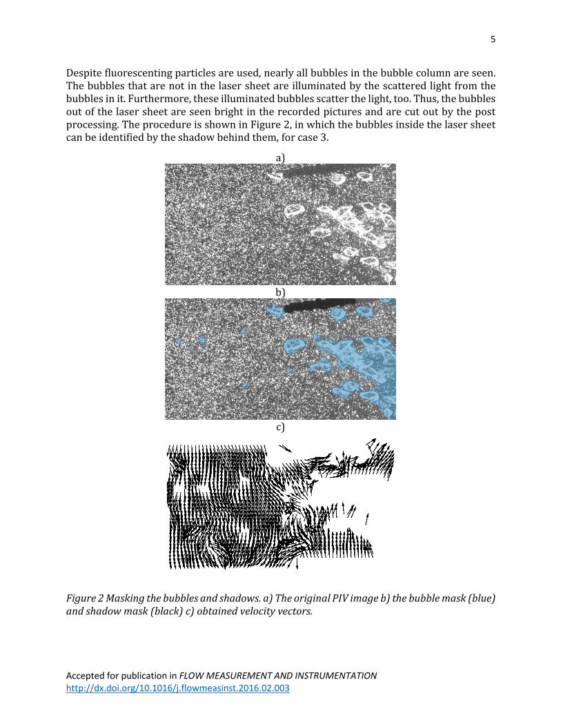
Despite fluorescenting particles are used, nearly all bubbles in the bubble column are seen. The bubbles that are not in the laser sheet are illuminated by the scattered light from the bubbles in it. Furthermore, these illuminated bubbles scatter the light, too. Thus, the bubbles out of the laser sheet are seen bright in the recorded pictures and are cut out by the post processing. The procedure is shown in Figure 2, in which the bubbles inside the laser sheet can be identified by the shadow behind them, for case 3.
a)
b)
c)
Figure 2 Masking the bubbles and shadows. a) The original PIV image b) the bubble mask (blue) and shadow mask (black) c) obtained velocity vectors.
Accepted for publication in FLOW MEASUREMENT AND INSTRUMENTATION http://dx.doi.org/10.1016/j.flowmeasinst.2016.02.003
4 Sampling Bias A sampling bias occurs if a not representative sample is picked, in which some values are less likely included than others. Such a not representative sample is picked by measuring the liquid velocity with PIV in bubbly flows. Bubbles that are passing the field of view hinder the view on the measuring plane as can be seen from Figure 2. However, these large bubbles drive the flow and, therefore, higher velocities occur just when many of these bubbles are in the field of view. Accordingly, these velocities that are connected to the bubbles are less likely measured. As a consequence, a sampling bias occurs. It should be noted, that the sampling bias is not caused by the bubbles inside the laser sheet, but by the bubbles out of it.
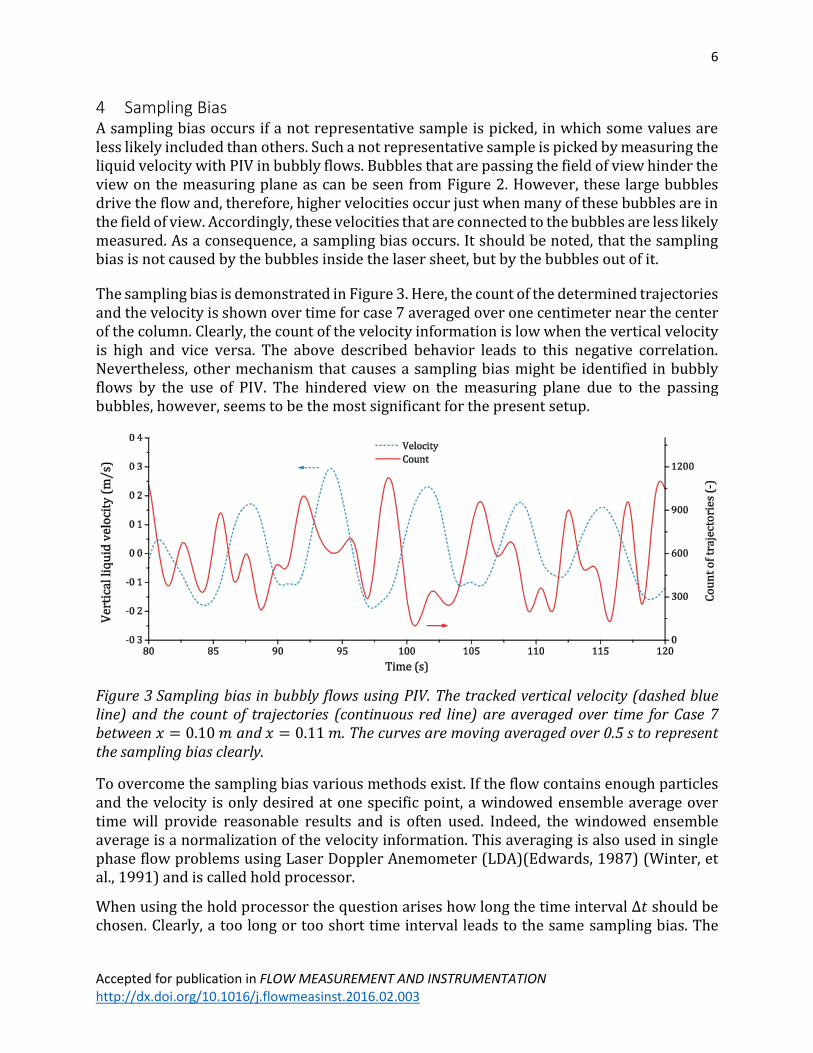
The sampling bias is demonstrated in Figure 3. Here, the count of the determined trajectories and the velocity is shown over time for case 7 averaged over one centimeter near the center of the column. Clearly, the count of the velocity information is low when the vertical velocity is high and vice versa. The above described behavior leads to this negative correlation. Nevertheless, other mechanism that causes a sampling bias might be identified in bubbly flows by the use of PIV. The hindered view on the measuring plane due to the passing bubbles, however, seems to be the most significant for the present setup.
Figure 3 Sampling bias in bubbly flows using PIV. The tracked vertical velocity (dashed blue line) and the count of trajectories (continuous red line) are averaged over time for Case 7 between 𝑥 = 0.10 𝑚 and 𝑥 = 0.11 𝑚. The curves are moving averaged over 0.5 s to represent the sampling bias clearly.
To overcome the sampling bias various methods exist. If the flow contains enough particles and the velocity is only desired at one specific point, a windowed ensemble average over time will provide reasonable results and is often used. Indeed, the windowed ensemble average is a normalization of the velocity information. This averaging is also used in single phase flow problems using Laser Doppler Anemometer (LDA)(Edwards, 1987) (Winter, et al., 1991) and is called hold processor.
When using the hold processor the question arises how long the time interval Δ𝑡 should be chosen. Clearly, a too long or too short time interval leads to the same sampling bias. The
Accepted for publication in FLOW MEASUREMENT AND INSTRUMENTATION http://dx.doi.org/10.1016/j.flowmeasinst.2016.02.003
problem is solved by choosing a variable time interval depending on the distribution of the velocity information over the measuring area.
In fact, the velocity information is not equally distributed over the measuring area. The count of the velocity information near the wall is twice as high as in the center. This is caused by a higher probability of the presence of bubbles in the center which hinder the field of view. Therefore, a simple hold processor that waits in time until a certain amount of trajectories are sampled is not meaningful.
The measuring area is discretized in grid cells and the hold processor waits the time Δ𝑡𝑖 until all grid cells are filled with at least one velocity information. Afterwards, the velocity is averaged over the time Δ𝑡𝑖 inside the grid cell. Indeed, the averaging over the grid cell is a windowed averaging in space. In the following this hold processor in space and time is written as ⟨𝑣𝑚⟩Δ𝑡𝑖
, with index 𝑚 denoting the grid cell.
Using this hold processor, the sampling bias is overcome. For investigation, a test function with an analytic solution can be defined, for example
The function described by Equation (4-1) is a discretized sine function. The discretization points 𝑗 are randomly distributed over the sine function by using a Gaussian distribution 𝔾(𝑛(𝑖))
𝑗. The sine function is also discretized in time which is denoted with 𝑖.
The Gaussian distributed total amount of 𝑛(𝑖) discretization points is also Gaussian distributed over time. The sine function is meandering in time by shifting the x-axis. The meandering Gaussian distribution simulate a problem similar to the one shown in Figure 3 with a positive correlation coefficient between sampling count (represented by the Gaussian distribution) and the measuring value (the sine function value y) . The correct average in continuous space over the steps 𝑖 of this test function is simply 𝑦(⟨𝑥𝑖⟩) = sin(𝑋𝜋 + ⟨𝑥𝑖⟩) + 𝑑.
The above defined hold processor ⟨𝑣𝑚⟩Δ𝑡𝑖
can be studied with this easy test function nicely.
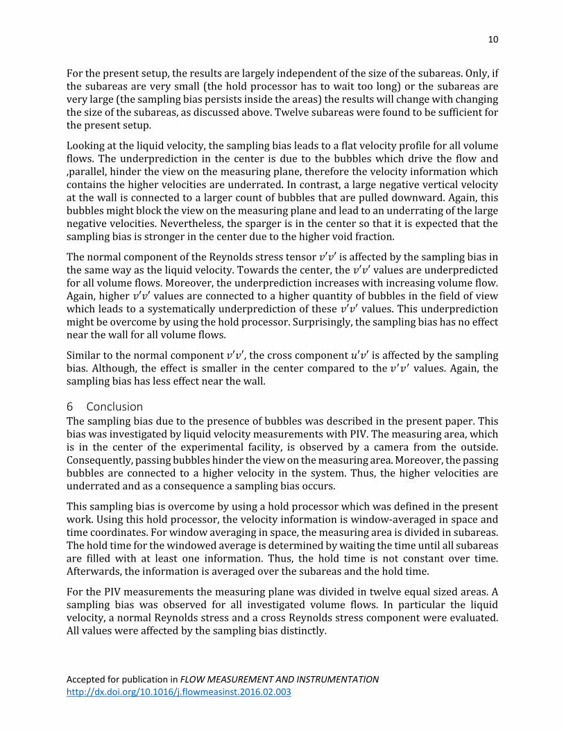
For example, using Δ𝑥 = 0.1 and 𝑑 = 0.5 the sine function is meandering in 0.1 𝜋⁄ steps around 0.5 with 𝑥𝑖 ∈ [−0.5,0.5]. Using 𝑠 = 50, the normalized averaged results obtained by using the hold processor, the simple ensemble averaging and the analytical solution are shown in Figure 4. Obviously, the hold processor can represent the averaged function. In contrast, the ensemble average cannot represent the averaged function.
Nevertheless, if the time step is too large or the hold processor have to wait too long the result will tend to the simple ensemble-averaged result. Obviously, the best results will be obtained if no waiting time is needed and only the information is windowed averaged in space due to the grid definition. However, if the grid cells are too large the sampling bias persists inside them.
Accepted for publication in FLOW MEASUREMENT AND INSTRUMENTATION http://dx.doi.org/10.1016/j.flowmeasinst.2016.02.003
Figure 4 Comparison of the hold processor with the simple ensemble averaging used on the analytical test function.
Turbulence parameters have to be formulated correctly when the hold processor is used. For example the turbulence kinetic energy 𝑘 is defined as
𝑘(𝑡) =1
2(𝑣𝑥
′ 𝑣𝑥′ + 𝑣𝑦
′ 𝑣𝑦′ + 𝑣𝑧
′𝑣𝑧′ ) . (4-2)
With 𝑣𝑘′ the fluctuation in the kth direction
𝑣𝑘′ (𝑡) = 𝑣𝑘(𝑡) − ⟨𝑣𝑘⟩ . (4-3)
Clearly, the hold processor must not be simply used on the turbulence kinetic energy or the fluctuation. Thus, the fluctuation in the m-th cell in the kth direction have to be written as
Moreover, the fluctuation must not be simply averaged over the hold time because the fluctuations with different sign would compensate each other. Consequently, the square of the fluctuation is averaged with the hold processor, hence the turbulence kinetic energy at the discrete time 𝑡𝑖 in the m-th cell is calculated by
𝑘𝑚(𝑡𝑖) =1
2(⟨𝑣𝑚,𝑥
′ 𝑣𝑚,𝑥′ ⟩Δ𝑡𝑖
+ ⟨𝑣𝑚,𝑦′ 𝑣𝑚,𝑦
′ ⟩Δ𝑡𝑖+ ⟨𝑣𝑚,𝑧
′ 𝑣𝑚,𝑧′ ⟩Δ𝑡𝑖
) . (4-5)
The same treatment is needed for all statistic variables.
Summarizing, a hold processor for problems with a sampling bias in space and time is derived. The windowed ensemble average in space is done by defining an Eulerian grid which is the natural averaging procedure for particle image velocimetry. The hold processor
Accepted for publication in FLOW MEASUREMENT AND INSTRUMENTATION http://dx.doi.org/10.1016/j.flowmeasinst.2016.02.003
waits the time until all grid cells are filled with at least one velocity information. Afterwards, the information, which the hold processor collected over time, are averaged inside the grid cells. Consequently, the average over the total time is calculated by the use of the arithmetic average of the values obtained from the windowed average. Naturally, if no sampling bias occurs and enough velocity information are available, the hold processor is equal to the ensemble average.
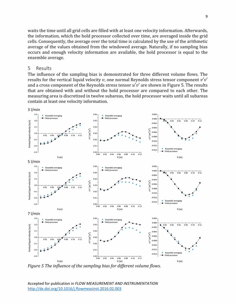
5 Results The influence of the sampling bias is demonstrated for three different volume flows. The results for the vertical liquid velocity 𝑣, one normal Reynolds stress tensor component 𝑣′𝑣′ and a cross component of the Reynolds stress tensor 𝑢′𝑣′ are shown in Figure 5. The results that are obtained with and without the hold processor are compared to each other. The measuring area is discretized in twelve subareas, the hold processor waits until all subareas contain at least one velocity information.
3 l/min
5 l/min
7 l/min
Figure 5 The influence of the sampling bias for different volume flows.
Accepted for publication in FLOW MEASUREMENT AND INSTRUMENTATION http://dx.doi.org/10.1016/j.flowmeasinst.2016.02.003
For the present setup, the results are largely independent of the size of the subareas. Only, if the subareas are very small (the hold processor has to wait too long) or the subareas are very large (the sampling bias persists inside the areas) the results will change with changing the size of the subareas, as discussed above. Twelve subareas were found to be sufficient for the present setup.
Looking at the liquid velocity, the sampling bias leads to a flat velocity profile for all volume flows. The underprediction in the center is due to the bubbles which drive the flow and ,parallel, hinder the view on the measuring plane, therefore the velocity information which contains the higher velocities are underrated. In contrast, a large negative vertical velocity at the wall is connected to a larger count of bubbles that are pulled downward. Again, this bubbles might block the view on the measuring plane and lead to an underrating of the large negative velocities. Nevertheless, the sparger is in the center so that it is expected that the sampling bias is stronger in the center due to the higher void fraction.
The normal component of the Reynolds stress tensor 𝑣′𝑣′ is affected by the sampling bias in the same way as the liquid velocity. Towards the center, the 𝑣′𝑣′ values are underpredicted for all volume flows. Moreover, the underprediction increases with increasing volume flow. Again, higher 𝑣′𝑣′ values are connected to a higher quantity of bubbles in the field of view which leads to a systematically underprediction of these 𝑣′𝑣′ values. This underprediction might be overcome by using the hold processor. Surprisingly, the sampling bias has no effect near the wall for all volume flows.
Similar to the normal component 𝑣′𝑣′, the cross component 𝑢′𝑣′ is affected by the sampling bias. Although, the effect is smaller in the center compared to the 𝑣′𝑣′ values. Again, the sampling bias has less effect near the wall.
6 Conclusion The sampling bias due to the presence of bubbles was described in the present paper. This bias was investigated by liquid velocity measurements with PIV. The measuring area, which is in the center of the experimental facility, is observed by a camera from the outside. Consequently, passing bubbles hinder the view on the measuring area. Moreover, the passing bubbles are connected to a higher velocity in the system. Thus, the higher velocities are underrated and as a consequence a sampling bias occurs.
This sampling bias is overcome by using a hold processor which was defined in the present work. Using this hold processor, the velocity information is window-averaged in space and time coordinates. For window averaging in space, the measuring area is divided in subareas. The hold time for the windowed average is determined by waiting the time until all subareas are filled with at least one information. Thus, the hold time is not constant over time. Afterwards, the information is averaged over the subareas and the hold time.
For the PIV measurements the measuring plane was divided in twelve equal sized areas. A sampling bias was observed for all investigated volume flows. In particular the liquid velocity, a normal Reynolds stress and a cross Reynolds stress component were evaluated. All values were affected by the sampling bias distinctly.
Accepted for publication in FLOW MEASUREMENT AND INSTRUMENTATION http://dx.doi.org/10.1016/j.flowmeasinst.2016.02.003
This sampling bias is important for all measuring techniques that are affected by the dispersed phase. However, the effect of the sampling bias has to be evaluated for every problem separately. The effect might be quantified by calculating the correlation coefficient of the measured value and the sample. For PIV measurements, the measured value is the velocity and the sample can be chosen to the count of the velocity information.
The derived hold processor, which was also tested by the use of analytical test functions, gave reasonable results. Distinct differences were observed by using the hold processor compared to not using the hold processor. Therefore, the quality of the velocity measurements in bubbly flows using PIV can be increased by using this hold processor. In general, high quality liquid velocity measurements are vitally needed for CFD validation (Ziegenhein, et al., 2015) (Ma, et al., 2015) (Masood, et al., 2014). In combination with the slotting method (Tummers & Passchier 1996) applied to particle laden flows (Poelma et al. 2006) it might be possible to obtain unbiased power density spectra in complex bubbly flows such as described in the present work. Moreover, the defined hold processor is not limited to liquid velocity measurements using PIV.
ACKNOWLEDGEMENT
This work was funded by the Helmholtz Association within the frame of the Helmholtz Energy Alliance “Energy Efficient Chemical Multiphase Processes” (HA-E-0004).
REFERENCES
Edwards, R. V., 1987. Report of the Special Panel on Statistical Particle Bias Problems in Laser
Anemometry. J. Fluids Eng., 109(2), pp. 89-93.
Hoesel, W. & Rodi, W., 1977. New biasing elimination method for laser‐Doppler velocimeter counter.
Rev. Sci. Instrum., Volume 48, pp. 910-919.
Hosokawa, S. & Tomiyama, A., 2013. Bubble-induced pseudo turbulence in laminar pipe flows. Int. J.
Heat Fluid Flow, Volume 40, pp. 97-105.
Jakobsen, M. L., Easson, W. J., Greated, C. A. & Glass, D. H., 1996. Particle image velocimetry: