Proceedings of the 22nd

National and 11th

International ISHMT-ASME Heat and Mass Transfer Conference

December 28-31, 2013, IIT Kharagpur, India

HMTC1300151

ON SOLUTION OF HYPERBOLIC EQUATION MODEL FOR ATMOSPHERIC DISPERSION

B. Ghosh Bhabha Atomic Research Centre Mumbai, Maharashtra, 400085

India bghosh@barc.gov.in

H.G. Lele Bhabha Atomic Research Centre Mumbai, Maharashtra, 400085

India hglele@barc.gov.in

R. K. Singh Bhabha Atomic Research Centre Mumbai, Maharashtra, 400085

India rksingh@barc.gov.in

ABSTRACT The dispersion of pollutant in the atmospheric boundary

layer is governed by varied degree of the fluctuating velocity

fields generated by atmospheric stability conditions. The

resulting propagation of the pollutant is more suitably

governed by the hyperbolic diffusion equation that the

conventional parabolic differential equation. In this study, the

dispersion of pollutant has been modeled under the boundary

layer parameterization by Monin-Obukhov (MO) stability

theory. Towards this end, the atmospheric velocity profile has

been obtained from MO stability parameterization. The

boundaries of the plume have been evaluated under different

atmospheric conditions. The vertical profiles of the

concentration distribution have been calculated from the

governing hyperbolic dispersion equation.

NOMENCLATURE β Isobaric thermal expansion coeffient

cp Isobaric specific heat

χ Pollutant concentration

D Molecular diffusion coefficient

ε Turbulent kinetic energy dissipation rate

g Acceleration due to gravity

H Height

k von Karman constant

K Exchange coefficient

L Monin-Obukhov length

Pr Prandtl number

q Ground heat flux

Q Quantity of release for instantaneous source

Ri Richardson number

ρ Ambient air density

t Time

T Temperature

τ Shear stress at ground

u Velocity vector

u Horizontal velocity in x-direction

w Vertical velocity in z-direction

x Position vector in space

ξ Non-dimensional x-coordinate

z Vertical coordinate

ζ Nondimensional z-coordinate

INTRODUCTION

There has been a great deal of work on turbulent diffusion

(see the treatise by Monin and Yaglom [1]). Turbulent

diffusion of a passive additive in an incompressible fluid is

usually described by the parabolic advection–diffusion

equation, proposed by Boussinesq [2] and Taylor [3],

( ){ }D.

DDD K S

tχ

χχ− ∇ + = (1)

where χ(x, t) is the concentration, D is the molecular diffusion

coefficient, KD(x, t) is the turbulent diffusion coefficient, Sχ is

the strength of the source of additive, D/Dt = ∂/∂t + u.∇ is the

advective time derivative and u(x, t) is the mean velocity of

the ambient fluid.

The parabolic character of the semi-empirical equation of

diffusion means that the contamination, upon exit from the

source, is instantaneously propagated in all directions and can

be discovered quickly, even though in completely negligible

quantity, at any large distance from the source. Usually, this

inadequacy is acceptable, since the volume inside which the

contamination concentration is not too small is always limited,

and the concentration distribution inside this volume is

generally satisfactorily described by the parabolic diffusion

equation (Monin [4]). However, in some cases (in particular,

close to the real boundary of the contamination cloud), use of

the parabolic diffusion equation can lead to significant errors.

For example, smoke issuing from a chimney of height h

reaches the ground at a distance from the pipe not less than

uh/w, where u is the wind velocity, v is the maximum velocity

of the propagation of the smoke along the vertical. In this

same time, according to the solution of the parabolic equation

of diffusion, the smoke is found at the surface of the earth

arbitrarily close to the chimney.

The generalization of the diffusion equation, which would

give this equation a hyperbolic character was initially

proposed Davydov [5], Goldstein [6], Davies [7] and Monin

[8-9]. Batchelor and Townsend [10] suggest that ‘a description

of the diffusion by some kind of integral equation is more to

be expected’ (p 360).

Meyers [11] has derived a three dimensional hyperbolic

differential equation based on finite correlated particle

velocities. This is appropriate for modeling anisotropic

turbulent diffusion in the atmosphere. Cauchy initial data, the

mean wind, the Reynolds stress tensor, and a typical frequency

of pulsation are required for complete solution. The outlines of

plumes and puffs may be obtained with only knowledge of the

Reynolds stress tensor and mean wind velocity. The classical

parabolic diffusion equations are a limiting form of this

hyperbolic model.

Ghoshal and Keller [12] derived hyperbolic equation,

analogous to the telegrapher’s equation in one dimension,

from an integro-differential equation for the mean

concentration which allows it to vary rapidly. If the mean

concentration varies sufficiently slowly compared with the

correlation time of the turbulence, the hyperbolic equation

reduces to the advection–diffusion equation. However, if the

mean concentration varies very rapidly, the hyperbolic

equation should be replaced by the integro-differential

equation.

Kasanski and Monin [13] filmed smoke plumes under

different stability conditions. Figure 1 shows the behaviour of

a smoke plume under neutral stability condition atmospheric

boundary layer. It is obvious from this figure that the smoke

cloud is confined with a bounded region which grows in the

down wind direction in a regular manner.

Fig.1 Smoke Plume under Neutral Atmospheric Stratification

The behaviour under unstable stratification is shown in

figure 3. Here the smoke plume appears to be more mixed up.

But, even then, the upper boundary of the cloud is clearly

identifiable.

Fig.2 Smoke Plume under Unstable Atmospheric Stratification

Thus, the diffusion of pollution in the atmosphere is due to

the turbulent pulsations of the wind velocity. The magnitude

of these pulsations is limited (for example, it does not exceed

the sound velocity); therefore, according to Monin [14], the

following guidelines may be observed: Propagation of the

pollution through space due to atmospheric diffusion occurs

with a limited velocity.

In this work, we analyse the behavior of pollution

dispersion in the atmospheric conditions characterised by

Monin-Obukhov (MO) similarity theory. Towards this goal,

we first study the atmospheric velocity and temperature

profiles under different atmospheric stability conditions as

dictated by Monin-Obukhov (MO) similarity principle. Then

we explore the limit of the boundary of smoke plume. Finally,

we undertake the calculation of concentration distribution

within the plume.

MO SIMILARITY THEORY AND ABL PROFILES

The portion of the Planetary Boundary Layer (PBL)

immediately adjacent to the surface, typically upto 100 m

from the ground, is called surface layer, and that above the

surface layer is called the Ekman layer. Within the surface

layer, the vertical turbulent fluxes of momentum and heat are

assumed constant with respect to height, and indeed they

define the extent of this region.

When the turbulence in the atmosphere is maintained by

buoyant production, the boundary layer is said to be in a

convective state. The source of buoyancy is the upward heat

flux originating from the ground heated by solar radiation.

Convective turbulence is relatively vigorous and causes rapid

vertical mixing in the atmospheric boundary layer.

Depending on state of turbulence in the atmospheric

boundary layer, the Atmospheric Boundary Layer (ABL) is

classified as: (1) neutral, (2) stable and (3) unstable (or

convective).

The stationary turbulent regime in the surface layer, when

the turbulence is homogeneous in the horizontal plane, obeys

the similarity theory developed by Monin and Obukhov [15].

ABL Similarity Parameters: The turbulent regime is completely determined by the

external parameters,

* /u τ ρ= and ( )pq cρ …(2)

which do not vary with altitude in the surface layer and by the

universal parameter g/T0 characterizing the effect of

Archimedes forces. T0 is the potential temperature. u* is the

friction velocity.

According to Monin-Obukhov (MO) similarity theory, in

the surface layer, the only scale of velocity is *u and the only

scale of length is

( )0

3

*

p

g q

T c

uL

k ρ

=−

,

0 for 0, unstable

for 0, neutral

0 for 0, stable

q

q

q

< >

→ ∞ →

> <

…(3)

where k is von Karman constant. The resulting length scale, L,

is known as Monin-Obukhov length.

The length scale L, first introduced by Obukbov [16], is an

important physical characteristic of the state of the surface

layer and can be called the height of the sub-layer of dynamic

turbulence.

The other derived external parameter is the temperature scale,

*

*

1

p

qT

ku cρ= − …(3)

Atmospheric Boundary Layer Profiles The nondimensional characteristics of the averaged field of

velocities and temperatures ( dd

kz uu zτ

and *

dd

TzT z

) should be

definite functions of the “external parameters” and of

coordinate z. The only non-dimensional combination which

we can make from g/T0, uτ, q/(ρcp), and z is z/L, from which it

follows that

d

dv

uu z

z kz L

τ ϕ

=

and *d

dT

T T z

z z Lϕ

=

…(4)

The equality of the resulting exchange coefficients implies

that

( ) ( ) ( )z z zv TL L L

ϕ ϕ ϕ= = …(5)

Keeping z and decrease magnitude q indefinitely, one

approaches the conditions of neutral stratification, which

correspond to infinite growth of the scale L (with respect to

absolute magnitude). Obviously, in this limit, we should retain

the relation velocity gradient for neutral condition, from which

it follows that

( )0 1ϕ = …(6)

It follows that in a stationary turbulent surface layer, the

wind and temperature profiles can be described using one

universal function of z/L.

The average velocity and temperature profiles are given

by,

0*( )zu z

u z f fk L L

= −

and 0*0( )

zT zT z T f f

k L L

= + −

…(7)

where z0 is the roughness and f(ζ) is the universal function.

where the universal function can be identified as,

( )( ) df

ζ ϕ ςζ ς

ς= ∫ …(8)

f(ζ) is, moreover, connected to the local Richardson number

through the relation,

Ri 1

Ri ( )c f ζ=

′ …(9)

Thus, exact functional form of f(ζ) depends on atmopheris

stability condition.

Surface Layer Profiles: In view of the limiting value in

equation (6) of φ(ζ), in the case |z/L| < 1 we can limit

ourselves to the first terms of the function φ(z/L) expanded in

a power series. As a consequence, f(ζ) takes the following log-

linear form

0( ) lnf cζ ζ ζ≈ + where c0 = 0.6. …(10)

For large positive ζ (the case of a stable stratification), the

function is asymptotically proportional to ζ, while for large

negative ζ (case of thermal convection), it is asymptotically

approaches a constant according to the law

f(ζ) = c1ζ-1/3

+ const. …(11)

In subsequent subsection, we will further elaborate the

causes and implications of these limiting behaviours.

Convective Condition: In this case, due to the lack of an

averaged wind, the friction stress, on average will be zero (uτ

= 0), while the turbulence regime is characterized by only the

parameters q > 0 and g/T0. The regime of purely thermal

turbulence is automodular (self-patterning) and rom

dimensional considerations we get

2/3

1/3

1 0

p

qT T c T

c gzρ∞

= +

where C is the non-dimensional (universal) constant and T∞ is

a constant which has a temperature dimension.

Therefore, in the case of purely thermal turbulence, the

universal function f(z/L) (determined to within an additive

constant) has the form

f(z/L) = c1(z/L)−1/3

+ const.; when z/L << -1.

It can easily be shown that the consequent augmentation of

the turbulent elements with an increase in height and

simultaneous increase in the intensity of the fluctuations

causes rapid increase in exchange coefficients with height.

Stable Stratification: Turbulence decays in this limiting

case of abrupt inversion with a vanishingly weak wind.

Moreover, in this case turbulent exchange between different

atmospheric layers is hampered and turbulence takes on a

local character; at rather high altitudes z >> L (or, to put it

another way, with strong stability, that is with small L > 0) the

turbulence characteristics evidently cannot be functions of the

distance z to the ground. Thus, we may consider that in the

case of stable stratification with an increase in height z, (or,

with an increase in stability, i.e., a decrease in L) the

coefficient of mixing K and the Richardson number Ri tend

toward certain constant values. Accordingly, there is a

(universal) value Ri* of the Richardson number, which is such

that when z/L >> 1,

Ri ~ Ri*.

From above condition and general relation (9) between profile

gradient and Richardson number, it follows that when z/L >>

1,

*

1const.

Ri

z zf

L L

≈ +

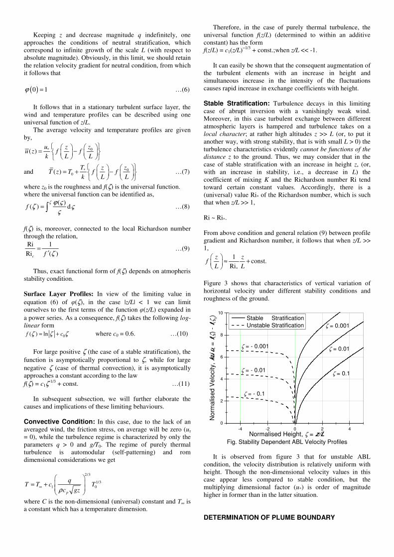
Figure 3 shows that characteristics of vertical variation of

horizontal velocity under different stability conditions and

roughness of the ground.

-4 -2 0 2 4

0

2

4

6

8

10

ζ = - 0.1

ζ = - 0.01

ζ = - 0.001

ζ = 0.001

ζ = 0.01

Norm

alis

ed V

elo

city,

ku/u

* = f

(ζ)

- f(

ζ 0)

Normalised Height, ζ = z/L

Stable Stratification

Unstable Stratification

ζ = 0.1

Fig. Stability Dependent ABL Velocity Profiles

It is observed from figure 3 that for unstable ABL

condition, the velocity distribution is relatively uniform with

height. Though the non-dimensional velocity values in this

case appear less compared to stable condition, but the

multiplying dimensional factor (u*) is order of magnitude

higher in former than in the latter situation.

DETERMINATION OF PLUME BOUNDARY

Here we explore the extent of pollutant cloud boundary

under the premises that: The turbulent diffusion in a

horizontally-homogeneous stationary surface layer of air

obeys the similarity theory in which the values L and *u are

the only scales of length and velocity.

The diffusion of pollution in the atmosphere is due to the

turbulent pulsations of the wind velocity. The magnitude of

these pulsations is limited (for example, it does not exceed the

sound velocity); therefore, according to Monin [14], it follows

that: Propagation of the pollution through space due to

atmospheric diffusion occurs with a limited velocity.

Accordingly, the space occupied by a smoke flowing out of

any source, has a very distinct boundary beyond which there is

no smoke. Such boundaries have been observed in

experiments conducted by Kasanski and Monin[13].

In conformity with MO similarity, the maximum velocity

of the vertical propagation of diffusing smoke is given by

*

* ( )w uλ φ ζ= …(12)

where ϕ(ζ) is a universal function, which can be subjected to

the condition ϕ (0) = 1 so that λ will be equal to *

* uw

under neutral stratification.

Kanaski and Monin [13] carried out experiment under

neutral condition from which, w* = 0.12 m/s and u* = 0.16

m/s, so that λ = 0.75.

In order to get the form of the function ϕ(ζ), let us use the

turbulent energy equation 2

0

d d

d dM H

u g TK K

z T zε

− =

…(13)

Rewriting this equation (13) in the form

2 2

0

d / d Ri1 1

(d / d ) (d / d ) Pr

H

M M M t

K g T z

K u z K T K u z

ε= − = −

and using the exchange relation, 2

*

d

dM

uu K

z=

4

*

Ri1

PrM tu K

ε= − …(14)

In accordance with similarity theory, 3*

t

w

lε ∝ and *

M tK w l∝ …(15)

where lt is the scale of turbulence.

Substituting these scaling relations and using the limiting

condition: w* ≈ 0 at Ri = Ric, we get

4

*

*

Ri Ri1 1

Pr Rit c

w

u

= − = −

As Prt can be equated to Ric, it becomes 4

*

*

Ri1

Ric

w

u

= −

…(16)

from which (using the relations (12) and (9)) 1/4 1/4

Ri 1( ) 1 1

Ri ( )c fφ ζ

ζ

= − = − ′

…(17)

When ζ is small and log-linear law of velocity profile is

valid,

( )1/4

1/41 1( ) 1 1 1

1/ 4φ ζ ζ ζ

ζ β

= − ≈ − ≈ −

+

The equations of motion of the smoke particles at the upper

boundary of the plume have the form

d

d

xu

t= and

*d

d

zw

t= …(18)

Substituting the u and w* profiles, the shape of the upper

boundary smoke plume is given by,

( )

( )0

* 1/4

/ ( / )d 1

d 1 1/ ( / )

f z L f z Lx u

z w k f z Lλ

−= =

′− …(19)

Integrating this differential relation (19) for plume

boundary, we arrive at the relation

−

=

L

z

L

hF

L

z

L

zF

k

Lx 00 ,,

λ; …(20)

where ( ){ }∫ ′−

−=

ζ

ζ

ζζ

ζζζζ

0

d)(/11

)()(,

4/1

00

f

ffF

Thus, the shape of the boundary of the smoke plume (in

particular, their inclination to horizon) does not depend upon

the wind velocity, but does depend upon the stratification of

the atmosphere.

The right hand side of relation (20) has been evaluated

through numerical integration under different atmospheric

stability conditions employing corresponding universal

functions. The numerical results are plotted in figure 4.

0 5 10 15 20

0

1

2

3

4

5

ζ0 = 0.1

ζ0 = 0.01

ζ0 = 0.001

ζ0 = - 0.001

ζ0 = - 0.01

Nondim

ensio

nal P

lum

e H

eig

ht,

ζ =

z/L

Nondimensional Distance, ξ = kλx/L

Stable Stratification

Untable Stratification

ζ0 = - 0.1

Fig.4: Plume Boundaries under Different ABL Conditions

It is obvious from figure 4 that vertical growth of the

plume boundary is much faster under unstable condition than

under stable stratifications. In the former case the growth

behavior is superlinear, whereas in the latter case it is

sublinear in nature.

CONCENTRATION PROFILE WITHIN THE PLUMES Guided by the principle of finite propagation velocity, we

are denied of the routine parabolic diffusion equation

corresponding to an infinitely rapid pollution propagation in

space. The transport equation corresponding to the limited

propagation velocity should be hyperbolic: such a hyperbolic

system of equations was obtained by Monin [8-9] in the form

0t z

χ ψ∂ ∂+ =

∂ ∂ and

**

2w

wt z

ψ χνψ

∂ ∂+ = −

∂ ∂ …(21)

where ψ is turbulent flux of the diffusing pollutant and ν is a

typical frequency of turbulent pulsations which in accordance

with the similarity principle can be written as 2 1/2* 2

*

*

1 d 1 1( ) 1

2 d 2 ( )

w u uf

u z k L f

λν ζ

ζ

′= = −

′ …(22)

The stationary solution of the hyperbolic system is given by, *

* ( )2

ww

z

χνψ

∂= −

∂

Approximating this relation as,

2

* *

d d

d d

u f

z u z ku z

χ ψ ψ∂= − = −

∂ …(23)

Integration of (23) lead to the relation,

11

*

( ) ( )z z

z z f fku L L

ψχ χ

− = − −

The full hyperbolic system can only be integrated numerically.

However, in the case of neutral stratification

*

* uw λ= and z

u

k

*

2

2

1 λν = …(24)

Then the hyperbolic system simplifies to,

0=∂

∂+

∂

∂

zt

ψχ and

zu

z

u

kt ∂

∂−=+

∂

∂ χλψ

λψ 2

*

2*

2

…(25)

The continuity and flux relation can be combined to yield

2 2

2 2t k t

ψ λ ψ ψ

ς ς

∂ ∂ ∂+ =

∂ ∂ ∂ …(26)

a telegraph equation in flux.

In terms of a transformed variable,

0( , )d

t

z t tψΨ = ∫ …(27)

The equation (26) transforms to 2 2

2 2t k t

λ

ς ς

∂ Ψ ∂Ψ ∂ Ψ+ =

∂ ∂ ∂ …(28)

Introducing a similarity variable, t/ςη = , the above

equation can be integrated to yield,

( )2 d1 const .

d k

λη

η

Ψ− − Ψ = …(29)

For instantaneous surface point source of intensity Q,

( ,0) δ( 0)z Q zψ = − …(30)

and for tutwz *

* λ=≥ , i.e., ς ≥ t or ,1≥η ψ = Ψ= 0.

Using the boundary condition, Ψ(η = 1) = 0,

( )2 d1

d k

λη

η

Ψ− = Ψ …(31)

Rearranging and carrying out further integration we obtain,

2

* *

1 1 .kz z

u t u t

λ

λ λ

Ψ ∝ − +

From continuity condition,

(0, )t QΨ =

we get.

2

* *

1 1 .kz z

Qu t u t

λ

λ λ

Ψ = − +

…(32)

From first equation of hyperbolic system,

0 0 0d d d

t t t

t t tt z z z

χ ψψ

∂ ∂ ∂ ∂Ψ= − = − = −

∂ ∂ ∂ ∂∫ ∫ ∫

or,

12

*

1* 2

*

1

( , ) .

1

k

k

z

u tQz t

ku tz

u t

λ

λ

λχ

λ

−

+

−

=

+

…(33)

which is valid for 0 ≤ tutwz *

* λ=≤ and λ ≥ 2k.

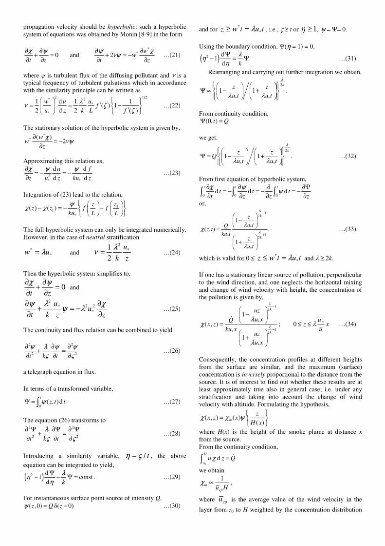
If one has a stationary linear source of pollution, perpendicular

to the wind direction, and one neglects the horizontal mixing

and change of wind velocity with height, the concentration of

the pollution is given by,

12

*

1* 2

*

1

( , )

1

k

k

uz

u xQx z

ku xuz

u x

λ

λ

λχ

λ

−

+

−

=

+

ɺ

; *0u

z xu

λ≤ ≤ …(34)

Consequently, the concentration profiles at different heights

from the surface are similar, and the maximum (surface)

concentration is inversely proportional to the distance from the

source. It is of interest to find out whether these results are at

least approximately true also in general case; i.e. under any

stratification and taking into account the change of wind

velocity with altitude. Formulating the hypothesis,

( , ) ( )( )

m

zx z x

H xχ χ ψ

=

where H(x) is the height of the smoke plume at distance x

from the source.

From the continuity condition,

0

dH

zu z Qχ =∫ ɺ

we obtain

1m

cpu Hχ ∝ ,

where cpu is the average value of the wind velocity in the

layer from z0 to H weighted by the concentration distribution

function, ψ(z/H). Taking H ∝ x and taking into consideration

that cpu vary with the distance very slowly, we obtain

m xχ ∝ .

Thus, the concentration profiles in a smoke plume at different

distances from the source are approximately similar to each

other. The maximum concentration in the smoke plume is

approximately inversely proportional to the distance from the

source.

0.0 0.2 0.4 0.6 0.8 1.0

0.0

0.2

0.4

0.6

0.8

1.0

Norm

aliz

ed C

oncentr

ation,

χku

*x/Q

Normalized Height, uz/(λu*x)

λ/k = 2.0

λ/k = 2.5

λ/k = 3.0

Fig.5: Vertical Distribution of Concentration

Figure 5 presents the vertical concentration profile for

different values constant of proportionality between the

characteristic vertical velocity and the friction velocity. The

concentrations decreases with height as observed in numerous

experiments reported in the literature. The concentration

profiles in a plume at different distances from the source are

approximately similar to each other. The maximum

concentration in the smoke plume is approximately inversely

proportional to the distance from the source.

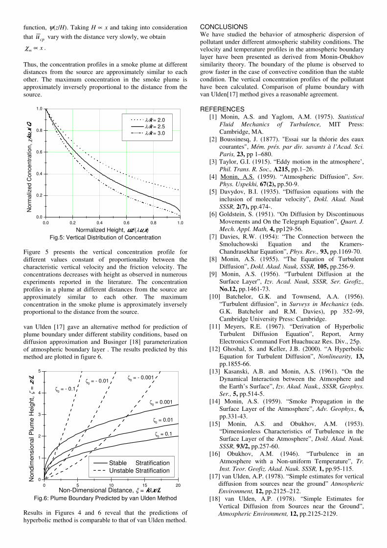
van Ulden [17] gave an alternative method for prediction of

plume boundary under different stability conditions, based on

diffusion approximation and Businger [18] parameterization

of atmospheric boundary layer . The results predicted by this

method are plotted in figure 6.

0

1

2

3

4

5

0 5 10 15 20

ζ0 = 0.1

ζ0 = 0.01

ζ0 = 0.001

ζ0 = - 0.001

ζ0 = - 0.01

Non-Dimensional Distance, ξ = kλx/L

Nondim

ensio

nal P

lum

e H

eig

ht,

ζ =

z/L

ζ0 = - 0.1

Stable Stratification

Unstable Stratification

Fig.6: Plume Boundary Predicted by van Ulden Method

Results in Figures 4 and 6 reveal that the predictions of

hyperbolic method is comparable to that of van Ulden method.

CONCLUSIONS We have studied the behavior of atmospheric dispersion of

pollutant under different atmospheric stability conditions. The

velocity and temperature profiles in the atmospheric boundary

layer have been presented as derived from Monin-Obukhov

similarity theory. The boundary of the plume is observed to

grow faster in the case of convective condition than the stable

condition. The vertical concentration profiles of the pollutant

have been calculated. Comparison of plume boundary with

van Ulden[17] method gives a reasonable agreement.

REFERENCES [1] Monin, A.S. and Yaglom, A.M. (1975). Statistical

Fluid Mechanics of Turbulence, MIT Press:

Cambridge, MA.

[2] Boussinesq, J. (1877). "Essai sur la théorie des eaux

courantes", Mém. prés. par div. savants à l’Acad. Sci.

Paris, 23, pp 1–680.

[3] Taylor, G.I. (1915). “Eddy motion in the atmosphere’,

Phil. Trans. R. Soc., A215, pp.1–26.

[4] Monin, A.S. (1959). “Atmospheric Diffusion”, Sov.

Phys. Uspekhi, 67(2), pp.50-9.

[5] Davydov, B.I. (1935). “Diffusion equations with the

inclusion of molecular velocity”, Dokl. Akad. Nauk

SSSR, 2(7), pp.474-.

[6] Goldstein, S. (1951). “On Diffusion by Discontinuous

Movements and On the Telegraph Equation”, Quart. J.

Mech. Appl. Math, 4, pp129-56.

[7] Davies, R.W. (1954): “The Connection between the

Smoluchowski Equation and the Kramers-

Chandrasekhar Equation”, Phys. Rev., 93, pp.1169-70.

[8] Monin, A.S. (1955). “The Equation of Turbulent

Diffusion”, Dokl. Akad. Nauk, SSSR, 105, pp.256-9.

[9] Monin, A.S. (1956). “Turbulent Diffusion at the

Surface Layer”, Izv. Acad. Nauk, SSSR, Ser. Geofiz.,

No.12, pp.1461-73.

[10] Batchelor, G.K. and Townsend, A.A. (1956).

“Turbulent diffusion”, in Surveys in Mechanics (eds.

G.K. Batchelor and R.M. Davies), pp 352–99,

Cambridge University Press: Cambridge.

[11] Meyers, R.E. (1967). “Derivation of Hyperbolic

Turbulent Diffusion Equation”, Report, Army

Electronics Command Fort Huachucaz Res. Div., 25p.

[12] Ghoshal, S. and Keller, J.B. (2000). “A Hyperbolic

Equation for Turbulent Diffusion”, Nonlinearity, 13,

pp.1855-66.

[13] Kasanski, A.B. and Monin, A.S. (1961). “On the

Dynamical Interaction between the Atmosphere and

the Earth’s Surface”, Izv. Akad. Nauk., SSSR, Geophys.

Ser., 5, pp.514-5.

[14] Monin, A.S. (1959). “Smoke Propagation in the

Surface Layer of the Atmosphere”, Adv. Geophys., 6,

pp.331-43.

[15] Monin, A.S. and Obukhov, A.M. (1953).

“Dimensionless Characteristics of Turbulence in the

Surface Layer of the Atmosphere”, Dokl. Akad. Nauk.

SSSR, 93/2, pp.257-60.

[16] Obukhov, A.M. (1946). “Turbulence in an

Atmosphere with a Non-uniform Temperature”, Tr.

Inst. Teor. Geofiz. Akad. Nauk. SSSR, 1, pp.95-115.

[17] van Ulden, A.P. (1978). “Simple estimates for vertical

diffusion from sources near the ground” Atmospheric

Environment, 12, pp.2125–212.

[18] van Ulden, A.P. (1978). “Simple Estimates for

Vertical Diffusion from Sources near the Ground”,

Atmospheric Environment, 12, pp.2125-2129.