ISSN 23473487

25 | P a g e S e p t 1 5 , 2 0 1 3

On Spectral-Homotopy Perturbation Method Solution of Nonlinear

Differential Equations in Bounded Domains

Ahmed A. Khidir

Faculty of Technology of Mathematical Sciences and Statistics

Alneelain University, Algamhoria Street, P.O. Box 12702, Khartoum - Sudan

E-mail: ahmed.khidir@yahoo.com

Abstract

In this study, a combination of the hybrid Chebyshev spectral technique and the homotopy perturbation method is used to

construct an iteration algorithm for solving nonlinear boundary value problems. Test problems are solved in order to

demonstrate the efficiency, accuracy and reliability of the new technique and comparisons are made between the obtained

results and exact solutions. The results demonstrate that the new spectral homotopy perturbation method is more efficient

and converges faster than the standard homotopy analysis method. The methodology presented in the work is useful for

solving the BVPs consisting of more than one differential equation in bounded domains.

Keywords: Chebyshev spectral method; Homotopy perturbation method; nonlinear boundary value problems.

Council for Innovative Research

Peer Review Research Publishing System

Journal: Journal of Advances in Physics

Vol. 1, No. 1

editor@cirworld.com

www.cirworld.com, member.cirworld.com

ISSN 23473487

26 | P a g e S e p t 1 5 , 2 0 1 3

1 Introduction

Many problems in the fields of physics, engineering and biology are modeled by coupled systems of boundary value

problems of ordinary differential equations. The existence and approximations of the solutions of these systems have been

investigated by many authors and some of them are solved using numerical solutions and some are solved using the

analytic solutions. One of these analytic solutions is the homotopy perturbation method (HPM). This method, which is a

combination of homotopy in topology and classic perturbation techniques, provides us with a convenient way to obtain

analytic or approximate solutions for a wide variety of problems arising in different fields. It was proposed first by the

Chinese researcher J. Huan He in 1998 [4,6]. The method has been applied successfully to solve different types of linear

and nonlinear differential equations such as Lighthill equation[4], Duffing equation [5] and Blasius equation [10], wave

equations [6], boundary value problems [11,12]. HPM method has been recently intensively studied by scientists and they

used it for solving nonlinear problems and some modifications of this method have published [13,14] to facilitate and

accurate the calculations and accelerate the rapid convergence of the series solution and reduce the size of work. The

application of the HPM in linear and non-linear problems has been developed by many scientists and engineers [7,8,9],

because this method continuously deforms some difficult problems into a simple problems which are easy to solve. The

limited selection of suitable initial approximations and linear operators and are some of the main limitations of the HPM.

Complicated linear operators and initial approximations may result in higher order differential equations that are difficult or

impossible to integrate using the standard HPM.

The purpose of the present paper to introduce a new alternative and improved of the HPM called Spectral Homotopy

Perturbation method (SHPM) in order to address some of the perceived limitations of the HPM uses the Chebyshev

pseudospectral method to solve the higher order differential equations. This study proposes a standard way of choosing

the linear operators and initial approximations for the SHPM. The obtained results suggest that this newly improvement

technique introduces a powerful for solving nonlinear problems. Numerical examples of nonlinear second order BVPs are

used to show the efficiency of the SHPM in comparison with the HPM. The new modification demonstrates an accurate

solution compared with the exact solution.

2 The Spectral-Homotopy Perturbation Method

For the convenience of the reader, we first present a brief review of the standard HPM. This is then followed by a

description of the algorithm of the SHPM solving nonlinear ordinary differential equations.

To illustrate the basic ideas of the HPM, we consider the following nonlinear differential equation

( ) ( ) = 0,A u f r r (1)

with the boundary conditions

, = 0,u

B u rn

(2)

where A is a general operator, B is a boundary operator, ( )f r is a known analytic function and is the boundary of

the domain . The operator A can, in generally, be divided into two parts L and part N so that equation (1) can be

written as

( ) ( ) ( ) = 0L u N u f r (3)

where L is a simple part which is easy to handle and N contains the remaining parts of A. By the homotopy technique

[2, 3], we construct a homotopy ( , ) : [0,1]v r p which satisfies

0( , ) = (1 )[ ( ) ( )] [ ( ) ( )] = 0, [0,1],H v p p L v L u p A v f r p r (4)

or

0 0( , ) = ( ) ( ) ( ) [ ( ) ( )] = 0H v p L v L u pL u p N v f r (5)

where [0,1]p is an embedding parameter, 0u is an initial approximation of equation (1), wich satisfies the boundary

conditions. Obviously, from equation (4) we have

ISSN 23473487

27 | P a g e S e p t 1 5 , 2 0 1 3

0( ,0) = ( ) ( ) = 0,H v L v L u (6)

( ,1) = ( ) ( ) = 0.H v A v f r (7)

The changing process of p from zero to unity is equivalent to the deformation of ( , )v r p from 0 ( )u r to ( )u r . In

topology, this is called deformation and 0( ) ( )L v L u , ( ) ( )A v f r are homotopic. We can assume that the solution

of equation (4) can be written as a power series in p , i.e.

2

0 1 2= ...v v pv p v (8)

setting =1p , results in the approximation to the solution of equation (1)

0 1 2

1

= = ...limp

u v v v v

(9)

The coupling of the perturbation method and the homotopy method gives the homotopy perturbation method (HPM),

which has eliminated limitations of the traditional perturbation methods.

To describe the basic ideas of the spectral-homotopy perturbation method, we consider the following second

order boundary value problem

( ) ( ) ( ) ( ) ( ) [ , ] = ( )u x a x u x b x u x N u x F x (10)

subject to the boundary conditions:

( 1) = (1) = 0u u (11)

where [ 1,1]x is an independent variable, ( ), ( )a x b x and ( )F x are known functions defined on [ 1,1] and N

is a nonlinear function. The differential equation (10) can be written in the following operator form:

[ ] [ ] = ( )u N u F xL (12)

where

2

2= ( ) ( )

d da x b x

dx dx L (13)

Here 0u is taken to be an initial solution of the nonhomogeneous linear part of governing differential equation (10) given

by:

0[ ] = ( )u F xL (14)

subject to the boundary conditions:

0 0( 1) = (1) = 0.u u (15)

Equation (14) together with the boundary conditions (15) can easily be solved using any numerical methods methods

such as finite differences, finite elements, Runge-Kutta or collocation methods. In this work we used the Chebyshev

spectral collocation method. This method is based on approximating the unknown functions by the Chebyshev

interpolating polynomials in such a way that the are collocated at the Gauss-Lobatto points (see [1,15] for details). The

unknown function 0 ( )u x is approximated as a truncated series of Chebyshev polynomials of the form

0 0

=0

( ) ( ) = ( ), = 0,1, , ,N

N

k k j

k

u x u x u T x j N (16)

where kT is the k th Chebyshev polynomial, ku are coefficients and 0 1, , , Nx x x are Gauss-Lobatto collocation

points defined on the interval [ 1,1] by

ISSN 23473487

28 | P a g e S e p t 1 5 , 2 0 1 3

= cos , = 0,1, ,jx j NN

(17)

The derivatives of the function 0 ( )u x at the collocation points are represented as

0

0

=0

( )= ( )

r Nr

kj jrk

d u xu x

dxD (18)

where r is the order of differentiation and D being the Chebyshev spectral differentiation matrix whose entries are

defined as (see for example,[1,15]);

2

2

00

( 1)= ; , = 0,1, , ,

= = 1,2, , 1,2(1 )

2 1= = .

6

j kj

jk

k j k

kkk

k

NN

cj k j k N

c x x

xk N

x

N

D

D

D D

(19)

Substituting Equations (16)-(18) in (14) yields

0( ) = ( ),Au x F x (20)

where

2= ( ) ( ) ,A a x b x I D D (21)

where I is a diagonal matrix of size N N . The matrix A has dimensions N N while matrix ( )F x has

dimensions 1N . To incorporate the boundary conditions (15) to the system (20) we delete the first and the last rows

and columns of A and delete the first and last elements of 0u and ( )F x , this showing as follows

0,0 0,1 0, 1 0, 0 0

1,0 1,

2,0 2,

,0 ,

,0 ,1 , 1 ,

( ) ( )

=

( ) ( )

N N

N

N N N

N N N

N N N N N N N N

A A A A u x F x

A A

A

A A

A A

A A A A u x F x

(22)

Thus, the solution 0u is determined from the equation

1

0 = ( ),u A F x (23)

where 0 ,u A and ( )F x are the modified matrices of 0 ,u A and ( )F x , respectively. The solution (23) provide us with

the initial approximation of the Equation (10). The higher approximations are obtained by construct a homotopy for the

government Equation (10) as follows

0 0( , ) = [ ] [ ] [ ] [ ] ( ) = 0,U p U u p u p N U F x H L L L (24)

ISSN 23473487

29 | P a g e S e p t 1 5 , 2 0 1 3

where [0,1]p is an embedding parameter and U is assumed a solution of equation (10) given as power series in

p as follows

2

0 1 2

=0

= ( ) ( ) ( ) ... = ( )n

n

n

U u x pu x p u x p u x

(25)

Substitute (25) into (24) and compare between the coefficients of ip of both sides of resulting equation, we have

= 0, =1,2,...,i iu i nL (26)

where

0 0

=0 =0

= ( 1) [ ] ( ) = 0, =1,2,...!

n ni

i ini

du N u F x N u i

n d

L (27)

where

0, = 1

=1, > 1

i

i

(28)

From the set of equations (26), the i th order approximation for =1,2,3,..i are given by the following system of

matrices

= ,i iAu (29)

subject to the boundary conditions

( 1) = (1) = 0,i iu u (30)

To incorporate the boundary conditions (30) to the system (29) we delete the first and the last rows and columns of A

and delete the first and last elements of iu and i . This reduces the dimension of A to ( 2) ( 2)N N and those

of iu and i to ( 2) 1N . Finally, the solution if is determined from the equation

1= ,i iu A (31)

where ,iu A and i are the modified matrices of ,iu A and i , respectively. The solutions for (29) provides us with

the highes order approximations of the governing equation (10). The series iu is convergent for most cases. However,

the convergence rate depends on the nonlinear operator of (10). The following opinions are suggested and proved by He

[16,17]

1. The second derivative of ( )N u with respect to u must be small because the parameter p may be relatively large,

i.e 1p .

2. The norm of 1 N

Lu

must be smaller than one so that the series converges.

This is the same strategy that is used in the SHPM approach. We observe that the main difference between the HPM

and the SHPM is that the solutions are obtained by solving a system of higher order ordinary differential equations in the

HPM while for the SHPM solutions are obtained by solving a system of linear algebraic equations that are easier to solve.

3 Solution of Test Problems

In this section, we illustrate the use of SHPM by solving systems of nonlinear boundary value problems whose exact

solutions are known.

ISSN 23473487

30 | P a g e S e p t 1 5 , 2 0 1 3

Problem 1:

Consider the nonlinear second order boundary value problem:

2 1

2 2 4 2 = 0,2

f xf f xff f (32)

subject to the boundary conditions

( 1) = (1) = 0.f f (33)

The exact solution for (32) is

2

1 1( ) = .

1 2f x

x

(34)

To apply the SHPM on this problem we may construct the homotopy:

0 0

1( , ) = [ ] [ ] [ ] ( ) = 0,

2F p F f p f p N F

H L L L (35)

where F is an approximate series solution of (32) given by

2

0 1 2= .F f pf p f (36)

and

2

2= 2 2.

d dx

dx dx L (37)

The initial approximation for the solution of (32) is obtained from the solution of the linear equation

0 0 0

12 2 = 0.

2f xf f (38)

subject to the boundary conditions

0 0( 1) = (1) = 0.f f (39)

The higher order approximations for (32) obtained by compared between the coefficients of , ( 1)ip i of both sides of

(35) to get the following system of matrices

=i iAf (40)

subject to the boundary conditions

( 1) = (1) = 0i if f (41)

where

1 1

0 1 1

=0 =0

1= ( 1) [ ] 4 2 , =1,2,...

2

i i

i j i j j i j

j j

L f x f Df f f j

(42)

Finally, the solution of (32) is given by substitute if s in (36) after setting =1p .

ISSN 23473487

31 | P a g e S e p t 1 5 , 2 0 1 3

Table 1: Comparison of the values of the SHPM (shaded) and HPM (unshaded) approximate solutions for ( )f x

with the exact solution for various values of x ..

x 4th order 5th order 6th order 7th order Exact

-0.9 0.052486 0.052486 0.052486 0.052486 0.052486

0.052441 0.052482 0.052486 0.052486

-0.7 0.171141 0.171141 0.171141 0.171141 0.171141

0.168303 0.170417 0.170956 0.171094

-0.5 0.299999 0.300000 0.300000 0.300000 0.300000

0.284180 0.294067 0.297775 0.299166

-0.3 0.417420 0.417430 0.417431 0.417431 0.417431

0.378111 0.399540 0.409291 0.413727

0 0.499959 0.499994 0.499999 0.500000 0.500000

0.437500 0.468750 0.484375 0.492188

0.2 0.461516 0.461535 0.461538 0.461538 0.461538

0.410496 0.437038 0.449778 0.455894

0.4 0.362065 0.362069 0.362069 0.362069 0.362069

0.335244 0.350802 0.357337 0.360082

0.6 0.235294 0.235294 0.235294 0.235294 0.235294

0.227584 0.232827 0.234505 0.235041

0.8 0.109756 0.109756 0.109756 0.109756 0.109756

0.109116 0.109641 0.109735 0.109752

Table 2: Maximum absolute errors of the approximate solution of ( )f x for test problem 1 for different values of N

N 2nd order 4th order 6th order 8th order

30 31.693407 10

54.090457 10 79.880795 10

82.386776 10

50 31.693407 10

54.090457 10 79.880795 10

82.386776 10

60 31.693407 10

54.090457 10 79.880795 10

82.386773 10

100 31.693407 10

54.090457 10 79.880794 10

82.386771 10

200 31.693407 10

54.090457 10 79.880795 10

82.386777 10

Table 1 gives a comparison of SHPM and HPM results at different orders of approximation against the exact solution

at selected values of x when = 40N for SHPM. It can be seen from Table 1, the HPM results converge slowly to the

exact solution while the SHPM results converge rapidly to the exact solution. The SHPM convergence is achieved up to 6

decimal places at the 6th order of approximation. It is clear that the results obtained by the present method are more

convergence to the exact solution compared to the HPM. As with most approximation techniques, the accuracy further

improves with an increase in the order of the SHPM approximations.

ISSN 23473487

32 | P a g e S e p t 1 5 , 2 0 1 3

Table 2: Maximum absolute errors of the approximate solution of ( )f x for test problem 1 for different values of N

N 2nd order 4th order 6th order 8th order

30 31.693407 10

54.090457 10 79.880795 10

82.386776 10

50 31.693407 10

54.090457 10 79.880795 10

82.386776 10

60 31.693407 10

54.090457 10 79.880795 10

82.386773 10

100 31.693407 10

54.090457 10 79.880794 10

82.386771 10

200 31.693407 10

54.090457 10 79.880795 10

82.386777 10

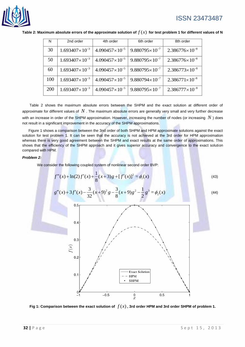
Table 2 shows the maximum absolute errors between the SHPM and the exact solution at different order of

approximate for different values of N . The maximum absolute errors are generally very small and very further decrease

with an increase in order of the SHPM approximation. However, increasing the number of nodes (or increasing N ) does

not result in a significant improvement in the accuracy of the SHPM approximations.

Figure 1 shows a comparison between the 3nd order of both SHPM and HPM approximate solutions against the exact

solution for test problem 1. It can be seen that the accuracy is not achieved at the 3rd order for HPM approximation

whereas there is very good agreement between the SHPM and exact results at the same order of approximations. This

shows that the efficiency of the SHPM approach and it gives superior accuracy and convergence to the exact solution

compared with HPM.

Problem 2:

We consider the following coupled system of nonlinear second order BVP:

2

1

1( ) ln(2) ( ) ( 3) [ ( )] = ( )

8f x f x x g f x x (43)

2 2 3

2

3 3 1( ) 3 ( ) ( 9) ( 9) = ( )

32 8 2g x f x x g x g g x (44)

Fig 1: Comparison between the exact solution of ( )f x , 3rd order HPM and 3rd order SHPM of problem 1.

ISSN 23473487

33 | P a g e S e p t 1 5 , 2 0 1 3

subject to the boundary conditions

( 1) = (1) = ( 1) = (1) = 0f f g g (45)

where

2 2

1

1 1( ) = ( 1) (2)ln

32 4x x (46)

2 3

2

1 3( ) = (225 69 45 7 ) ln(2)

128 2x x x x (47)

The exact solutions for ( )f x and ( )g x are

3 1

( ) = ln ( 1) ln(2)2 2

xf x x

(48)

3 2

( ) =4 3

xg x

x

(49)

The initial approximations of (43) and (44) are solutions of the following system of equations

0 0 0 1

1( ) ln(2) ( ) ( 3) = ( )

8f x f x x g x (50)

2

0 0 0 2

3( ) 3 ( ) ( 9) = ( )

32g x f x x g x (51)

subject to the boundary conditions

0 0 0 0( 1) = (1) = ( 1) = (1) = 0f f g g (52)

Applying the Chebyshev spectral collocation method we obtain the following system of matrices

0 0 0 0=T T

A F G P Q (53)

where

2

2 2

1ln(2) [( 3)]

8=

33 ( 9)

32

D D diag x

A

D D diag x

(54)

0 0 0 0 1 0 0 0 0 0 1 0= [ ( ), ( ),..., ( )], = [ ( ), ( ),..., ( )]N NF f x f x f x G g x g x g x (55)

and

0 0 0 0 1 0 0 1 0 1 1 1= [ ( ), ( ),..., ( )], = [ ( ), ( ),..., ( )]N NP x x x Q x x x (56)

where diag[ ] is a diagonal matrix of size N N and T is the transpose. The matrix A has dimensions 2 2N N

while matrices 0 0[ ]TF G and 0 0[ ]TP Q have dimensions 2 1N . To implement the boundary conditions (52) to the

system (53) we delete the first, , 1N N and the last rows of A, we also delete the first, N , 1N and last elements of

0 0[ ]TF G and 0 0[ ]TP Q . The first, , 1N N and the last columns of A are also deleted. This reduce the dimensions

ISSN 23473487

34 | P a g e S e p t 1 5 , 2 0 1 3

of A to 2( 2) 2( 2)N N , and reduce the dimensions of 0 0[ ]TF G and 0 0[ ]TP Q to 2( 2) 1N . The solution

0F and 0G for the system (53) gives the first approximations of the system equations (43) and (44) for ( )f x and ( )g x

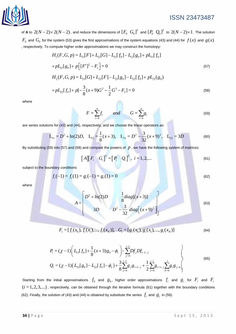
, respectively. To compute higher order approximations we may construct the homotopy:

1 11 12 11 0 12 0 11 0( , , ) = [ ] [ ] [ ] [ ] [ ]H F G p L F L G L f L g pL f

2

12 0 1[ ] [ ] = 0pL g p F F (57)

2 21 22 21 0 22 0 21 0( , , ) = [ ] [ ] [ ] [ ] ( )H F G p L G L F L g L f pL g

2 3

22 0 2

3 1[ ] [ ( 9) ] = 0

8 2pL f p x G G F (58)

where

=0 =0

= =n n

i i

i i

F f and G g (59)

are series solutions for (43) and (44), respectively, and we choose the linear operators as:

2 2 2

11 12 21 22

1 3= ln(2) , = ( 3), = ( 9) , = 3

8 32D D x D x D L L L L (60)

By substituting (59) into (57) and (58) and compare the powers of p , we have the following system of matrices:

= , =1,2,...T T

i i i iA F G P Q i (61)

subject to the boundary conditions

( 1) = (1) = ( 1) = (1) = 0i i i if f g g (62)

where

2

2 2

1ln(2) [( 3)]

8=

33 ( 9)

32

D D diag x

A

D D diag x

(63)

0 1 0 1= [ ( ), ( ),..., ( )], = [ ( ), ( ),..., ( )]i i i i N i i i i NF f x f x f x G g x g x g x (64)

1

11 0 0 1 1

=0

1 1

21 0 22 0 2 1 1

=0 =0 =0

1= ( 1) [ ] ( 3)

8

3 1= ( 1) [ ] [ ]

8 2

i

i j i j

j

ji i

i j i j i j i j k

j j k

P L f x g Df Df

Q L g L f g g g g g

(65)

Starting from the initial approximations 0f and 0g , higher order approximations if and ig for iF and iF

( =1,2,3,...)i , respectively, can be obtained through the iterative formula (61) together with the boundary conditions

(62). Finally, the solution of (43) and (44) is obtained by substitute the series if and ig in (59).

ISSN 23473487

35 | P a g e S e p t 1 5 , 2 0 1 3

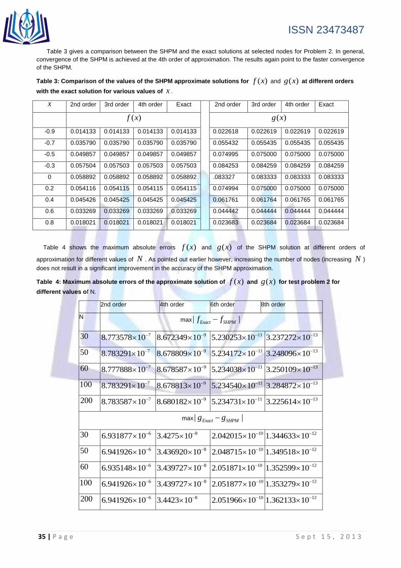
Table 3 gives a comparison between the SHPM and the exact solutions at selected nodes for Problem 2. In general,

convergence of the SHPM is achieved at the 4th order of approximation. The results again point to the faster convergence

of the SHPM.

Table 3: Comparison of the values of the SHPM approximate solutions for ( )f x and ( )g x at different orders

with the exact solution for various values of x .

x 2nd order 3rd order 4th order Exact 2nd order 3rd order 4th order Exact

( )f x ( )g x

-0.9 0.014133 0.014133 0.014133 0.014133 0.022618 0.022619 0.022619 0.022619

-0.7 0.035790 0.035790 0.035790 0.035790 0.055432 0.055435 0.055435 0.055435

-0.5 0.049857 0.049857 0.049857 0.049857 0.074995 0.075000 0.075000 0.075000

-0.3 0.057504 0.057503 0.057503 0.057503 0.084253 0.084259 0.084259 0.084259

0 0.058892 0.058892 0.058892 0.058892 .083327 0.083333 0.083333 0.083333

0.2 0.054116 0.054115 0.054115 0.054115 0.074994 0.075000 0.075000 0.075000

0.4 0.045426 0.045425 0.045425 0.045425 0.061761 0.061764 0.061765 0.061765

0.6 0.033269 0.033269 0.033269 0.033269 0.044442 0.044444 0.044444 0.044444

0.8 0.018021 0.018021 0.018021 0.018021 0.023683 0.023684 0.023684 0.023684

Table 4 shows the maximum absolute errors ( )f x and ( )g x of the SHPM solution at different orders of

approximation for different values of N . As pointed out earlier however, increasing the number of nodes (increasing N )

does not result in a significant improvement in the accuracy of the SHPM approximation.

Table 4: Maximum absolute errors of the approximate solution of ( )f x and ( )g x for test problem 2 for

different values of N.

2nd order 4th order 6th order 8th order

N max | |Exact SHPMf f

30 78.773578 10 98.672349 10

115.230253 10 133.237272 10

50 78.783291 10 98.678809 10

115.234172 10 133.248096 10

60 78.777888 10 98.678587 10

115.234038 10 133.250109 10

100 78.783291 10 98.678813 10

115.234540 10 133.284872 10

200 78.783587 10 98.680182 10

115.234731 10 133.225614 10

max | |Exact SHPMg g

30 66.931877 10 83.4275 10

102.042015 10 121.344633 10

50 66.941926 10 83.436920 10

102.048715 10 121.349518 10

60 66.935148 10 83.439727 10

102.051871 10 121.352599 10

100 66.941926 10 83.439727 10

102.051877 10 121.353279 10

200 66.941926 10 83.4423 10

102.051966 10 121.362133 10

ISSN 23473487

36 | P a g e S e p t 1 5 , 2 0 1 3

(a) (b)

Fig 2: Comparison of the exact solution ( )f x and ( )g x of test problem 2 with 2nd order SHAM solutions.

Figure 2 shows a comparison between the exact solution for ( )f x and ( )g x against the 2nd order SHPM

approximate solutions for Problem 2. Again, we note that there is good agreement between the exact solutions and the

SHPM approximations even at very low orders of approximation.

4 Conclusion

In this paper, we have shown that the proposed SHPM can be used successfully for solving nonlinear boundary value

problems in bounded domains. The merit of the SHPM is that it converges faster to the exact solution with a few terms

necessary to obtain accurate solution, this was demonstrated through examples which proved the convergency of the

SHPM, it was also found that is has best selection method to the initial approximation than HPM.

The main conclusions emerging from this study are follows:

1. SHPM proposes a standard way of choosing the linear operators and initial approximations by using any form of

initial guess as long as it satisfies the boundary conditions while the initial guess in the HPM can be selected that will

make the integration of the higher order deformation equations possible.

2. SHPM is simple and easy to use for solving the nonlinear problems and useful for finding an accurate approximation

of the exact solution because the obtained governing equations are presented in form of algebraic equations.

3. SHPM is highly accurate, efficient and converges rapidly with a few iterations required to achieve the accuracy of the

numerical results compared with the standard HPM, for example, in this study it was found that for a few iterations of

SHPM was sufficient to give good agreement with the exact solution.

Finally, the spectral homotopy perturbation method described above has high accuracy and simple for nonlinear

boundary value problems compared with the standard homotopy perturbation method. Because of its efficiency and easy

of use. The extension to systems of nonlinear BVPs allows the method to be used as alternative to the traditional Runge-

Kutta, finite difference, finite element and Keller-Box methods.

REFERENCES

[1] L. N. Trefethen, Spectral Methods in MATLAB, SIAM, 2000.

[2] S. J. Liao, An approximate solution technique not depending on small parameters: a special example, Int. J. Non-

linear Mechanics, 30(3),(1995) 371-380.

[3] S. J. Liao, Boundary element method for general nonliear differential operator, Engineering Analysis with boundary

element, 20(2), (1997) 91-99.

[4] J. H. He, Homotopy perturbation method: a new nonlinear analytical technique, Appl. Math. Comput., 135, (2003), 73-

79.

[5] J. H. He, Application of homotopy perturbation method to nonlinear wave equations, Chaos, Solitons Fractals, 26,

(2005), 695-700.

[6] A. Belendez, C. Pascual, T. Belendez, A. Hernandez, Solution for an anti-symmetric quadratic nonlinear oscillator by

a modified He's homotopy perturbation method, Nonlinear Anal. RWA, in press (doi:10.1016/j.nonrwa.2007.10.002).

ISSN 23473487

37 | P a g e S e p t 1 5 , 2 0 1 3

[7] L. Cveticanin, Homotopy perturbation method for pure nonlinear differential equation, Chaos Solitons Fractals 30 (5),

(2006), 1221-1230.

[8] F. Shakeri, M. Dehghan, Solution of the delay differential equations via homotopy perturbation method, Math.

Comput. Modelling, 48, (2008) 486–498.

[9] J. H. He, A simple perturbation approach to Blasius equation, Appl. Math. Comput. 140, (2003) 217-222.

[10] J. H. He, Homotopy perturbation method for solving boundary value problems, Phys. Lett. A 350, (2006) 87-88.

[11] A. Y ld r m, Solution of BVPs for fourth-order integro-differential equations by using homotopy perturbation method,

Comput. Math. Appl. 56(12), (2008) 3175-3180.

[12] OZ. M. dibat, A new modification of the homotopy perturbation method for linear and nonlinear operators. Appl. Math.

Comput. 189, (2007), 746-753.

[13] A. Belendez, C. Pascual, T. Belendez, A. Hernandez, Solution for an anti-symmetric quadratic nonlinear oscillator by

a modified He's homotopy perturbation method. Nonlinear Anal.: Real World Appl. (2007).

doi:10.1016/j.nonrwa.2007.10.002

[14] C. Canuto, M. Y. Hussaini, A. Quarteroni, T. A. Zang, Spectral Methods in Fluid Dynamics, Springer-Verlag, Berlin,

(1988).

[15] J. H. He, Homotopy perturbation technique, Comput. Methods Appl. Mech. Eng., 178, (1999) 257–262.

[16] J. H. He, Homotopy perturbation method: a new nonlinear analytical technique, Appl. Math. Comput., 135, (2003),

73–79.