On stiffness in affine asset pricing models - Singapore Management

Journal of Computational Finance (99–123) Volume 10/Number 3, Spring 2007

On stiffness in affine asset pricing models

Shirley J. HuangLee Kong Chian School of Business, Singapore Management University,50 Stamford Road, Singapore 178899; email: [email protected]

Jun YuSchool of Economics and Social Sciences, Singapore Management University,90 Stamford Road, Singapore 178903; email: [email protected]

Economic and econometric analysis of continuous-time affine asset pricingmodels often necessitates solving systems of ordinary differential equations(ODEs) numerically. Explicit Runge–Kutta (ERK) methods have beensuggested to solve these ODEs both in the theoretical finance literatureand in the financial econometrics literature. In this paper we show thatunder many empirically relevant circumstances the ODEs involve stiffness,a phenomenon which leads to some practical difficulties for numericalmethods with a finite region of absolute stability, including the whole classof ERK methods. The difficulties are highlighted in the present paper in thecontext of pricing zero-coupon bonds as well as econometric estimation ofdynamic term structure models via the empirical characteristic function. Toovercome the numerical difficulties, we propose to use implicit numericalmethods for the ODEs. The performance of these implicit methods relativeto certain widely used ERK methods are examined in the context ofbond pricing and parameter estimation. The results show that the implicitmethods greatly improve the numerical efficiency.

1 INTRODUCTION

“· · · around 1960, things became completely different and everyonebecame aware that world was full of stiff problems.”

Dahlquist (1985)

When valuing financial assets in a continuous-time, arbitrage-free framework,one often needs to find the numerical solution to a partial differential equation(PDE) (examples include the Feynman–Kac PDE for bond prices; see Duffie

Both authors gratefully acknowledge financial support from the Research Office at SingaporeManagement University. We would like to thank the anonymous referee for constructivecomments that have substantially improved the article. We also wish to thank John Butcher,David Chen, Peter Phillips, Dai Min and participants in the Econometric Society WorldCongress in London, 2005 International Symposium on Econometrics Development in Beijing,the Inaugural Saw Centre for Financial Studies Conference on Quantitative Finance and theSingapore Econometric Study Group Meeting for comments on an earlier version of the paper.All computations were performed using MATLABr12 and Compact Visual FORTRAN 6.6a.

99

100 S. J. Huang and J. Yu

(2001) for details and references). Given the fact that in many practically rel-evant cases solving the PDE is computationally demanding and even becomesimpractical when the number of states is modestly large, considerable attentionhas been paid to the class of affine asset pricing models where the risk-neutraldrift and volatility functions of the process for the state variables are affine. Underthe affine specification, many asset prices have either completely or nearly closed-form expressions. Important examples from the first category include Black andScholes (1973) for pricing equity options, Vasicek (1977) and Cox, Ingersoll, andRoss ((1985); hereafter CIR) for pricing bonds and bond options, and Heston(1993) for pricing equity and currency options. Important examples from thesecond category include Duffie and Kan (1996) for pricing bonds, Chacko andDas (2002) for pricing interest derivatives, Bates (1996) for pricing currencyoptions, and Duffie et al (2000) for a treatment of very general pricing relations.The solutions have nearly closed-form expressions in the sense that the PDE isdecomposed into a system of ordinary differential equations (ODEs) and henceonly a system of ODEs, as opposed to a PDE, has to be solved numerically.Such decomposition greatly facilitates the numerical implementation of pricing(Piazzesi (2003)).

Computational burdens are even heavier for econometric analysis ofcontinuous-time dynamic asset pricing models based on discretely sampledobservations. The reasons for this are: (i) the implied transition density ofdiscretely sampled observations are solutions to PDEs which have to be solvednumerically at every data point and at each iteration in the numerical optimizations(examples include the apparent need to solve the Kolmogorov forward andbackward equations for the transition density in the maximum likelihood (ML)approach; see Lo (1988) for details and references1); (ii) as argued above, theasset prices themselves are numerical solutions to PDEs. However, the additionalaffine specification of the drift and volatility functions of the state process underthe physical measure will greatly facilitate econometric estimation of continuous-time models via the empirical characteristic function (ECF). In particular, in aninfluential study Duffie et al (2000) showed that the conditional characteristicfunction (CCF) of the state variable(s) and hence the CCF of the observable(s)have nearly closed-form expressions for the class of affine models in the sensethat only a system of ODEs has to be solved, although the likelihood functionsare more difficult to obtain. Exploiting these nearly closed-form expressions ofCCF, Singleton (2001) proposed several estimation procedures based on the ECFand CCF, circumventing the numerical problem in solving the PDEs. Yu (2004)provides a detailed review of the literature on the estimation problem via the ECF.

Due to the specific functional form of the ODEs found in the literature (ie,the so-called Ricatti equations), it is generally believed by many researchersthat these ODEs can be solved fast and numerically efficiently using traditional

1In a recent contribution, however, Aït-Sahalia and Kimmel (2003) showed that it is nolonger necessary to solve the Kolmogorov forward and backward equations to implement theapproximate ML approach of Aït-Sahalia (2003).

Journal of Computational Finance Volume 10/Number 3, Spring 2007

On stiffness in affine asset pricing models 101

numerical solvers for initial problems, such as explicit Runge–Kutta method.Specifically, Piazzesi (2003) recommended the MATLAB command ode452 tosolve the ODEs.3 In spite of its high order of accuracy, like any other explicitRunge–Kutta (ERK) method, ode45 has a finite region of absolute stability (seeHuang (2005) for a detailed discussion of stability of Runge–Kutta methods andButcher (2003) for a textbook treatment). The stability properties of numericalmethods are important for obtaining a good approximation to the true solution. Asis known, at each mesh point there are differences between the exact solution andthe numerical solution, known as the error. Sometimes the accumulation of theerror will cause instability and the numerical solution will no longer follow thepath of the true solution. Therefore, a method must satisfy the stability conditionso that the numerical solution will converge to the exact solution. In this paper,we show that under many situations that are empirically relevant in finance, theODEs involve stiffness; that is, there are processes in the system with significantlydifferent time scales (Dahlquist and Björck (1974)). In the term structure ofinterest rates literature, a typical finding in multi-factor models is that one factorhas a very slow mean reversion and another has a much faster reverting rate; see,for example, Chen and Scott (1993), Geyer and Pichler (1999), and Jagannathanet al (2003). Moreover, in the financial volatility literature, it is empirically foundthat, when two volatility factors are used, one factor corresponds to the shortmemory component which has a very fast decay rate and the other correspondsto a long memory component which has a very slow decay rate; see, for example,Chernov et al (2003) and Engle and Lee (1999). In both cases, the processes inthe system have very different time scales and hence exhibit stiffness. When anexplicit method is used to solve a stiff problem, a small stepsize has to be chosento ensure stability and hence the algorithm becomes numerically inefficient.

To address the problem of computational inefficiency of ERK methods for stiffsystems, this paper introduces implicit numerical methods which ensure the so-called A-stability (that is, the stability region includes all of the left half-plane;see Section 2 for the formal definition). In particular, we examine the performanceof two implicit methods in two different contexts. The two implicit methodsconsidered are an implicit Runge–Kutta method and an implicit linear multistepmethod. In the first context we price zero-coupon bonds, while in the secondcontext we estimate an affine term structure model. While implicit methods havereceived much attention in the recent numerical ODE literature (see Huang (2005)for a survey on implicit methods) and have been extensively used in engineering,physics, and chemistry (Aiken (1985)), to the best of our knowledge, we know ofno earlier application in the finance literature.

As the proposed implicit solvers have an unbounded stability region, thestepsize can be large or small, depending on the degree of stiffness. This flexibility

2It is an order four embedded in order five Runge–Kutta method; see Shampine and Reichelt(1997) for details.3From personal communications, we have found that many researchers who are working in thisarea have used ode45 to solve the Ricatti equations numerically.

www.journalofcomputationalfinance.com


in the choice of the stepsize makes the procedures numerically more efficient thanthe ERK methods when the underlying system involves stiffness. For example,when a 20-year zero coupon bond is priced under a stiff three-factor model, wefind that an implicit method is about 70 times more efficient than ode45. Moredetails of this implementation and comparison are provided in Section 4.

Compared with the situation in asset pricing, the numerical efficiency wouldbe more of an issue in the econometric analysis of continuous-time affine modelsvia the ECF. This is because: (i) estimation requires numerical optimizationsand at each iteration in the numerical optimizations a system of ODEs has tobe solved numerically; (ii) pricing only requires solving one system of ODEs,which is associated with the risk-neutral measure, to be solved whereas estimationrequires an additional system of ODEs, which is associated with the physicalmeasure, to be solved. Our finding indicates that, without sacrificing the statisticalefficiency of parameter estimates, the implicit methods substantially reduce thecomputer time when a stiff two-factor CIR model and a three-factor affine modelare estimated.

This paper is organized as follows. Section 2 defines the stiffness for initialvalue problems, reviews general approaches for non-stiff and stiff problems, anddiscusses the stability properties of numerical solvers. Section 3 explains thepractical relevance of stiffness in the context of asset pricing and econometricestimation. In Section 4 we compare the performance of implicit methods withERK methods in the two contexts. Section 5 concludes and outlines some furtherapplications of implicit methods.

2 STIFFNESS AND IMPLICIT METHODS

2.1 What is stiffness?

Any initial problem of ODEs can be classified into one of two types, non-stiff andstiff. Although the difference between the two types of problems is not clear cut,stiffness is widely found (Aiken (1985)) in many applied sciences such as robotics,fluid dynamics, electric circuits, and chemical kinetics. However, to the best ofour knowledge, stiffness has not been reported in finance. Several attempts at arigorous definition of stiffness have been made in the numerical analysis literature.In this paper, we follow the definition of Gear (1971, p. 209).

DEFINITION 1 Stiff differential equations are differential equations with greatlydiffering time constants (ie, rates of decay).

Since, in a stiff system, some components of the solution decay much morerapidly than the others, for a numerical method with a finite region of stability, weare forced to use excessively small stepsizes in relation to the smoothness of thesolution, which inevitably decreases computational efficiency and accumulatesmore machine roundoff error. As a result, stiffness leads to some practicaldifficulties for explicit methods.



To illustrate the problem, we consider the following simple, hypotheticalexample,

dy1(t)

dt= y1(t)− 2y2(t) (1)

dy2(t)

dt= 1,001y1(t)− 1,002y2(t) (2)

with initial conditions y1(0)= 1 and y2(0)= −1. This linear system has thefollowing exact solution,

(y1(t)

y2(t)

)= 1,003

999

(11

)e−t − 2,002

999

2

1,001

1

e−1,000t (3)

The component of the solution involving the term e−1,000t decays very fastwhereas the other component involving e−t decays very slowly. This feature canobviously be captured by the Jacobian matrix of the ODEs

(1 −2

1,001 −1,002

)

which has two distinct eigenvalues λ1 = −1, λ2 = −1,000, and hence the systemcan be rotated into a system of two independent differential equations,

dz(t)

dt= −z(t) (4)

dw(t)

dt= −1,000w(t) (5)

To explain the numerical difficulty of explicit methods, we consider the explicitEuler method (other explicit methods share the same spirit) and obtain

wn+1 = (1 − 1,000h)wn = (1 − 1,000h)n+1w(0) (6)

where h is the stepsize and wn+1 is the numerical approximation to w((n+ 1)h).Note that the exact solution decays as t increases, thus the numerical solutionshould do the same. This clearly requires that |1 − 1,000h|< 1 and hence 0<h < 0.002 for a real value of h to fulfill the stability requirement. For this reason,we say the explicit Euler method has a finite region of absolute stability. It is clearthat after a few steps, the magnitude of w(t) will be very small compared withz(t) which still contains the significant information that we are interested in.

Formally, for a linear problem y ′(t)= λy(t) with λ < 0, the stability region ofthe explicit Euler method is given by |1 + z| ≤ 1 where z= λL with L being a lagoperator. The stability region is plotted in Figure 1.

Stiffness can be understood in the following linear system

y ′(t)=My(t) (7)



FIGURE 1 Stability region of explicit Euler method (shaded area).

2 0

i

i

where M is an N × N matrix which has distinct eigenvalues λj (j = 1, . . . , N).The system can be rotated into a system of N independent differential equations

z′(t)= diag(λ1, . . . , λN)z(t) (8)

The solution of the above equation is of the form

z(t)= (C1 eλ1t , . . . , CN eλN t )� (9)

where the Ci are constants which depend on the initial conditions. Let Re(·) be thereal part of a complex number. If Re(λj ) < 0 for j = 1, . . . , N , then Ci eλi t → 0when t → ∞. Consider the case where these eigenvalues are very different, forexample, one of the eigenvalues has a very negative real part relative to the others.This means that

R = maxj |Re(λj )|minj |Re(λj )| � 1 (10)

Denote maxj |Re(λj )| by λ0. Hence, the exponential function exp(λ0t) decays tozero much more rapidly than the function based on the eigenvalue, minj |Re(λj )|.As a result, the system is difficult to solve for explicit methods. The ratio R iscalled the “stiffness ratio” which provides a measure of stiffness (only eigenvalueswith negative real parts are considered).

As many ODEs encountered in continuous-time finance are actually non-linear,it is useful to generalize the stiffness ratio to non-linear systems:

y ′(t)= f (y(t)), f : RN → RN

y0 = y(t0)

For non-linear systems the Jacobian is used to determine the stiffness. If theeigenvalues of the Jacobian J = ∂f /∂y (an N × N matrix of partial derivatives,



∂fi/∂yj ) satisfy the same condition as in (10), then the initial value problem isstiff. In general, there are two types of error introduced by a numerical method,truncation error and roundoff error. On the one hand, stability requires the use ofa small stepsize for the component with the fastest rate, which of course decreasesthe truncation error. On the other hand, the choice of a small stepsize leadsto a large number of steps and hence long computer time. Moreover, becauseroundoff error will accumulate, after a large number of steps there will be alarge accumulation of roundoff error for the slowest moving component wherethe derivatives are small and relatively constant. Clearly, for a stiff system, thetrade-off is between large stepsizes to reduce computer time and roundoff errorand small stepsizes to reduce truncation error.

2.2 A-stability and implicit methods

In this section we review certain numerical solvers and their properties that arerelevant in finance, paying particular attention to the so-called A-stability and itslinkage to implicit methods.

We begin the review with the definition of order. For any point tn, let Y denotethe approximation of y(tn). For some positive integer p, if we have ‖Y (tn)−y(tn)‖/hp bounded, then we would define “the numerical solution to be of orderp”. If p is the highest value such that ‖Y (tn)− y(tn)‖/hp is bounded, we woulddefine “the order of the numerical solution to be p”. A comparison of the Eulersolution Y (tn) with the Taylor series of y(tn) gives the order of the Euler methodas at least 1.

The Euler method discussed above is explicit. The next formula is referred toas the implicit Euler method,

yn = yn−1 + hnf (yn), n= 1, 2, . . . , N, y0 = y(t0) (11)

It is implicit as Equation (11) is an implicit function in yn. The stability regionfor the implicit method is |1 − z| ≥ 1, which is shown in Figure 2. Obviously thestability region of the implicit Euler method is unbounded.

Runge–Kutta methods can be understood as one way to generalize the Eulermethod. They allow for a multiplicity of evaluations of function f within onestep, and then use the information obtained to match a Taylor series expansionup to some higher order. For an ODE system y ′ = f (y), a general Runge–Kuttamethod is of the form

Yi = yn−1 + h

s∑j=1

aijf (Yj ), i = 1, . . . , s (12)

yn = yn−1 + h

s∑i=1

bif (Yi) (13)

where the quantities Y1, Y2, . . . , Ys are called stage values, which are approx-imations to solution values y(tn−1 + cih) at points tn−1 + cih. The integer s is



FIGURE 2 Stability region of implicit Euler method (unshaded area).

��

��

i

i

0 2

the number of stages of the method. The ci represent the position of the internalstages within one step. The Runge–Kutta formula can be conveniently representedby Butcher tableau,

c A

b�

where A= {aij }, b� = {bi}, and c= {ci}. The set of numbers aij are the coef-ficients used to find the internal stages using linear combinations of the stagederivatives. The components of the vector b are coefficients which represent howthe numerical solution at this step depends on the derivatives of the internal stages.The vector c = [c1, c2, . . . , cs]� is called the abscissae. If matrix A is strictlylower triangular, ie, the internal stages can be calculated without depending onlater stages, the method is explicit.

One widely used ERK method was proposed by Dormand and Prince (1980)(ode45 is the corresponding MATLAB command). Another example of ERKmethods was proposed by Bogacki and Shampine (1989) (ode23 is the cor-responding MATLAB command). It is of smaller order than ode45, but maybe more efficient at crude tolerances and in the presence of moderate stiffness(Shampine and Reichelt (1997)).

A well-known result in the numerical ODE literature (see, for example, Butcher(2003)) is that an ERK method with order p has the stability function of

R(z)= 1 + z+ z2

2! + · · · + zp

p! +O(zp+1) (14)

which determines the stability region of the underlying method via

S = {z ∈ C : |R(z)| ≤ 1}Journal of Computational Finance Volume 10/Number 3, Spring 2007


FIGURE 3 The boundaries of the stability regions of ERK of order one, two,three, four, correspond to f (z)= 1 + z+ z2/2! + · · · + zp/p! with p = 1, 2, 3, 4.In each case the stability region is the bounded set enclosed by these curves.

5 4 3 2 1 0 1 2 3

3

2

1

0

1

2

3

p=1

p=2

p=3

p=4

As a result, all ERK methods have bounded stability regions. The stability regionsof order one, two, three, and four ERK methods with p = 1, 2, 3, 4 are givenin Figure 3. It can be seen that although the stability region of a higher-orderERK method is slightly wider than that of the explicit Euler method, it is stillhighly restrictive. This will create, as shown above, numerical inefficiency forstiff systems. To deal with stiffness, a method with a much wider stability regionis called for. A typical approach in the numerical ODE literature is to use a methodwith an unbounded stability region. This is the motivation behind the concept ofA-stability (Dahlquist (1963)).

DEFINITION 2 A method whose stability region contains the whole of the lefthalf-plane is called A-stable.

Since all of the ERK methods have bounded stability regions, obviously theyare not A-stable (Iserles (1996)). In a ground-breaking paper, Dahlquist (1963)showed that explicit linear multistep methods cannot be A-stable either. Theseresults lead to the following recommendation: for a stiff problem, it is alwaysbetter to use implicit procedures; see, for example, Dahlquist and Björck (1974)and Huang (2005).



A simple implicit method is the implicit Euler method defined by Equation(11). As already demonstrated in Figure 2, the stability region of the implicitEuler method includes the whole half-plane and hence is A-stable. For the Runge–Kutta methods, if matrix A in the Butcher tableau is not strictly lower triangular,the method is implicit. A particular type of implicit Runge–Kutta method is themodified Rosenbrock method of Zedan (1990). The MATLAB code ode23simplements the method of order two.

Another way to generalize the Euler method is the use of linear multistepmethods. The idea is to use several previous solutions and derivative values incomputing the updated solution. The general form of a linear k-step method foran ODE y ′ = f (y) is

yn = α1yn−1 + · · · + αkyn−k + h(β0f (yn)+ · · · + βkf (yn−k))

where yn is the numerical approximation to the exact solution at the pointtn and α1, α2, . . . , αk, β0, β1, . . . , βk are fixed numbers. The values of α1,α2, . . . , αk, β0, β1, . . . , βk are chosen to obtain the highest possible order andcharacterize a method. If β0 = 0 and βi = 0, i = 1, . . . , k, the methods areobviously implicit and known as backward difference formulae (BDF; see, forexample, Gear (1971)). A closely related implicit linear multistep method isbased on the numerical differential formulae (NDF) of Klopfenstein (1971). TheMATLAB code ode15s is a variable order solver which implements these twosets of formulae, with the default being NDF.

3 STIFFNESS IN ASSET PRICING MODELS

Affine asset pricing models have recently received much attention both in thetheoretical finance literature and in the financial econometrics literature. Importantcontributions in this area include Duffie and Kan (1996), Dai and Singleton(2000), Duffie et al (2000), and Singleton (2001).

3.1 Stiffness in zero-coupon bonds

The multi-factor affine term structure model, introduced in Duffie and Kan (1996)and empirically investigated in Dai and Singleton (2000), adopts the followingspecifications.

1. Under the risk-neutral measure, the state variables, denoted by Y (t)=(Y1(t), . . . , YN(t))

�, follow an affine diffusion,

dY (t)= K̃(θ̃ − Y (t)) dt +� diag(√αj + β�

j Y (t)) dW̃ (t)

where K̃ and� areN × N matrices, αj is an scalar, βj is anN-dimensionalvector, for j = 1, . . . , N , and W̃ (t) is an N-dimensional independentstandard Brownian motion under the risk-neutral measure.



2. The short rate is an affine function of Y (t),

r(t)= δ0 + δ�y Y (t)

3. The market price of risk associated with factor j takes the form of

λj(t)= λj

√αj + β�

j Y (t) (15)

The specification implies that the physical measure of state variables has theaffine form of

dY (t)=K(θ − Y (t)) dt +� diag(√αj + β�

j Y (t)) dW(t)

where W(t) is an N-dimensional independent standard Brownian motion underthe physical measure, K = K̃ − ��, θ =K−1(K̃θ̃ +�ψ), with the j th row inmatrix � being given by λjβj and the ith element in vector ψ being given byλjαj .

Under these three assumptions, the yield-to-maturity at time t of a zero-couponbond that matures at t + τ takes the following affine expression (Duffie and Kan(1996)),

y(t; τ)= −A(τ)τ

+ B(τ)�

τY (t)= a(τ)+ b(τ)�Y (t) (16)

where A(τ), B(τ) satisfy a system of N + 1 ODEs (known as Ricatti equations)

dA(τ)

dτ= −θ̃�K̃�B(τ)+ 1

2

N∑j=1

[��B(τ)]2jαj − δ0 (17)

dB(τ)

dτ= −K̃�B(τ)− 1

2

N∑j=1

[��B(τ)]2jβj + δy (18)

with initial conditions A(0)= 0 and B(0)= 0. Note that the assumption aboutmarket price of risk in Equation (15) is more than enough for deriving the affinepricing relation in Equation (16). This assumption was relaxed in Duffee (2002)and further relaxed in Duarte (2004) without changing the pricing result.

It is known that the above affine model may not be econometrically identified.Dai and Singleton (2000) defined a model to be “maximal” if it has the maximumnumber of identifiable parameters and if it generates admissible (ie, well-defined)dynamics of state vectors. To find the maximal model, Dai and Singleton classifiedthe affine models into N + 1 subfamilies according to the number “m” of theY that determines the conditional variance of Y . Dai and Singleton called thissubfamily Am(N) and illustrated the idea in the case of N = 3. For example, the



maximum A1(3) model (called A1(3)Max) takes the form

dν(t)

dθ(t)dr(t)

=

µ 0 0

0 ν 0κrν −κ κ

ν̄θ̄θ̄

−

ν(t)θ(t)

r(t)

dt +

η 0 0ησθν 1 σθrησrν σrθ 1

×

√ν(t) 0 00

√ζ 2 + βθν(t) 0

0 0√αr + ν(t)

dWν(t)

dWθ(t)

dWr(t)

(19)

So,

α1 = α2 = ζ 2, α3 = αr, β1 =1

00

, β1 =

βθ0

0

, β3 =

1

00

As a result,

K̃ = µ+ ηλ1 0 0ησθνλ1 + λ2βθ + λ3σθr ν 0κrν + ηλ1σrν + λ2βθσrθ −κ κ

With suitable restrictions on certain parameters, one obtains the A1(3)BDFS

and A1(3)DS models. For example, if κrν = σθν = σrθ = σrθ = αr = β = 0, theA1(3)Max model becomes the A1(3)BDFS model.

The maximum A2(3) model (called A2(3)Max) takes the form

dν(t)

dθ(t)dr(t)

=

µ κνθ 0κθν ν 0κrν κrθ − κ κ

ν̄θ̄r̄

−

ν(t)θ(t)

r(t)

dt +

η 0 0

0 ζ 0ησrν ζσrθ 1

×

√ν(t) 0 00

√θ(t) 0√

αr + βθν(t)+ θ(t) 0 0

dWν(t)

dWθ(t)

dWr(t)

(20)

As a result,

K̃ = µ+ ηλ1 κrθ 0

κrθ ν + ζλ2 0κrν + λ1ησrν + λ3 κrθ − κ + λ2ζσrθ + λ3βθ κ

With suitable restrictions on certain parameters, one obtains the A2(3)Chen andA2(3)DS models. For example, if κνθ = σrθ = αr = βθ = 0, the A2(3)Max modelbecomes the A2(3)DS model.

Dai and Singleton (2000) further empirically estimated and tested two maximalthree-factor models and some of the restricted specifications in each of the twofamilies. Using the empirical results reported by Dai and Singleton, we findthe stiffness in the ODEs (18). For example, the estimates of (µ, η, λ1, ν, κ) inthe A1(3)BDFS model are (0.602, 0.007197, 67,900, 0.0523, 2.05). Using these



estimates we obtain

K̃ = 489.3 0 0

0 0.0523 0230,617.2 −2.05 2.05

Three eigenvalues of K̃ are 489.3, 0.0523, 2.05 which lead to a stiffness ratioof 9,355.6 in (18). For another example, the estimates of (µ, η, λ1, ν, ζ, λ2, κ)

in the A2(3)DS model are (0.636, 0.0109, 13,000, 0.103, 0.055857, −152, 2.7).Using these estimates we obtain

K̃ = 142.45 0 0

−33.9 −8.387 0−26,537.3 −2.7 2.7

The implied stiffness ratio is 52.76 and hence there is mild stiffness involved.

3.2 Stiffness in parameter estimation

Based on the assumption that the state variables Y (t) follow an affine diffusionunder the following physical measure

dY (t)=K(θ − Y (t)) dt +� diag(√αj + β�

j Y (t)) dW(t)

Duffie et al (2000) derived the CCF of Yt+1 conditional on Yt :

cY(t)(r)= E[exp(ir�Y (t + 1))|Y (t)] = exp(C(1)+D(1)�Y (t)) (21)

where i = √−1, r is the transform variable which takes real values, and C(·)andD(·) satisfy the following complex-valued ODEs (which are Ricatti equationsonce again):

dC(τ)

dτ= θ�K�D(τ)+ 1

2

N∑i=1

[��D(τ)]2jαj (22)

dD(τ)

dτ= −K�D(τ)+ 1

2

N∑i=1

[��D(τ)]2jβj (23)

with initial conditions C(0)= 0 and D(0)= ir .4

Under an affine pricing environment where y(t; τ) = a(τ)+ b(τ)�Y (t), theCCF of y(t + 1; τ) conditional on y(t; τ) is given by

cy(t)(r)= exp(ir�a(τ))cY(t)(b(τ)r) (24)

Exploiting this nearly closed-form solution for the CCF of y(t), Singleton(2001) and Chacko and Viceira (2003) proposed several estimation methods based

4The ODEs were given as a boundary problem by Duffie et al (2000). Piazzesi (2003) and Yu(2004) provided equivalent initial value representations for C(τ) and D(τ).



on the ECF. Yu (2004) provided a detailed review of these methods and moregenerally the literature on the parameter estimation via the ECF.

Stiffness may be present in the ODEs (23). For example, taking the estimatesreported in Geyer and Pichler (1999), the stiffness ratio is 2,847.2 in the estimatedfive-factor CIR model. The estimates reported in Chen and Scott (1991, 1992)for a two-factor CIR model imply a stiffness ratio of 351.9. These numbersindicate the presence of modest to severe stiffness. The implied stiffness ratiosin A1(3)BDFS, A1(3)DS, and A1(3)Max of Dai and Singleton (2001) are 39.2,77.0, and 78.9, respectively. The implied stiffness ratios in A2(3)Chen, A2(3)DS,and A2(3)Max of Dai and Singleton are 28.9, 26.2, and 40.7, respectively. Thesenumbers indicate the presence of mild stiffness.

4 PERFORMANCE OF NON-STIFF SOLVERS AND STIFF SOLVERS

To investigate the numerical inefficiency of ERK methods for stiff systems andto compare the performance of explicit solvers with implicit solvers, we focus ona two-factor CIR model (ie, an A2(2) model) and a three-factor affine model ofBalduzzi et al (1996) (ie, the A1(3)BDFS model).

4.1 A two-factor CIR model

There are several reasons why we use the two-factor CIR model to study thenumerical efficiency. First, the CIR model is a special case of affine models.As a result, the bond price can be calculated by solving a system of real-valuedODEs and the CCF can be obtained by solving a system of complex-valued ODEs.Second, the CIR model has a closed-form expression for bond prices, enabling anexamination of approximation errors of alternative numerical methods for bondpricing. Third, the model has only two factors so that a large-scale Monte Carlostudy of parameter estimation via the ECF is computationally feasible.

In particular, we design two experiments, one for pricing bonds and the otherfor estimating model parameters. In both experiments, we use four numericalsolvers for ODEs, two ERK methods, one implicit Runge–Kutta method and oneimplicit linear multistep method. The two explicit methods are ode45 and ode23while the two implicit methods are ode23s and ode15s. All four methods arebuilt-in functions in MATLAB.

The two-factor CIR model has two independent factors, each evolving overtime according to a square-root process:

dYi(t)= κi(µi − Yi(t)) dt + σiY1/2i (t) dWi(t), i = 1, 2 (25)

The market price of risk for each factor is assumed to be λiY1/2i (t). As a result the

risk-neutral measure is

dYi(t)= (κi + λi)

(κiµi

κi + λi− Yi(t)

)dt + σiY

1/2i (t) dW̃i(t), i = 1, 2 (26)



TABLE 1 Computational efficiency of explicit and implicit solvers for bong pricingunder the two-factor CIR model. CPU is the CPU time in seconds when the systemis solved repeatedly 5,000 times, Yield is the yield-to-maturity, and Stepsize is theaverage value of stepsizes.

10-year bond 20-year bond

CPU (s) Yield Stepsize CPU (s) Yield Stepsize

ode45 310 0.097471474 0.025 562 0.0978857433 0.026ode23 237 0.097471469 0.077 367 0.0978857286 0.080ode23s 122 0.097471778 0.345 115 0.0978866689 0.667ode15s 82 0.097470910 0.218 82 0.0978864351 0.417

Exact 0.097471410 0.0978857088

The instantaneous default-adjusted rate is assumed to be the sum of the two statevariables:

r(t)= Y1(t)+ Y2(t)

The parameters in the two experiments are set to be

κ1 = 0.06, µ1 = 0.03, σ1 = 0.03, λ1 = −0.01

andκ2 = 100, µ2 = 0.02, σ2 = 0.1, λ2 = −70

so that

K =(

0.06 00 100

)and K̃ =

(0.05 0

0 30

)

Obviously there exists severe stiffness in the ODEs (18) and ODEs (23) withstiffness ratios of 600 and 1,667, respectively.

4.1.1 Comparison for pricing bondsUsing the two-factor CIR model, we price two long-term bonds with maturitiesof 10 and 20 years. Both the analytical and numerical approaches are used tocompute the yields of zero-coupon bonds. The analytical expression for prices ofzero-coupon bonds is obtained from CIR (1985) and used to calculate the exactvalues for the yields. The numerical calculation is performed in MATLAB. Theinitial state variables are assumed to take the values of 0.03 and 0.02. To obtainthe CPU time, we follow the suggestion made by a referee of replicating theexperiment 5,000 times. Table 1 shows the CPU time (in seconds) on a Pentium-M laptop (1,600 MHz), the yield, and the average value of stepsizes used by eachsolver.

First, all four methods provide very accurate yields for both bonds. Second,although ode45 and ode23 are slightly more accurate, the marginal improve-ment in precision comes with higher computational cost. Compared with ode15s,for instance, ode45 is nearly a factor of three and six less efficient for thetwo bonds while ode23 is nearly a factor of two and three and a half times



TABLE 2 Computational efficiency and statistical efficiency of explicit and implicitsolvers for parameter estimation under the two-factor CIR model. CPU is theaveraged CPU time in seconds. The first number in each cell is the mean of theestimates while the second number is the standard deviation of the estimates.

κ1 µ1 σ1 λ1 κ2 µ2 σ2 λ2 CPU (s)

True 0.06 0.03 0.03 −0.01 100 0.02 0.1 −70ode45 0.0903 0.0292 0.0308 −0.0088 105.9 0.0205 0.096 −66.5 28,578.0

0.0100 0.0055 0.0101 0.0068 11.30 0.0041 0.0255 9.11ode23 0.0902 0.0293 0.0307 −0.0088 105.9 0.0206 0.096 −66.8 21,619.1

0.0099 0.0055 0.0102 0.0068 11.31 0.0040 0.0252 9.08ode23s 0.0903 0.0293 0.0305 −0.0086 105.8 0.0207 0.097 −66.6 10,152.6

0.0099 0.0054 0.0103 0.0069 11.32 0.0041 0.0256 9.10ode15s 0.0904 0.0294 0.0304 −0.0087 105.9 0.0205 0.096 −66.8 6,460.2

0.0099 0.0055 0.0102 0.0069 11.29 0.0040 0.0252 9.09

less efficient. The longer the maturity, the less the relative efficiency of theexplicit methods. Third, the improvement in numerical efficiency by the implicitmethods is manifest in the average value of stepsizes used by each solver. For bothbonds, the two explicit methods use much smaller stepsizes than the two implicitmethods. This is because the ODE is stiff and the ERK methods must choosesmall enough stepsizes to ensure stability. Moreover, when the maturity increases,the stepsize increases nearly in the same proportion for the two implicit methodswhile it remains constant for the two explicit methods. Therefore, it is expectedthat the computational efficiency of the implicit methods relative to the explicitmethods increases with the maturity and with the stiffness.

4.1.2 Comparison for parameter estimationIn this section we estimate the two-factor CIR model based on 600 discretelysampled observations on six-month and 10-year zero-coupon bonds that aresimulated from the same model. We repeat the experiment 1,000 times. As before,the numerical calculation is performed in MATLAB. Although the likelihoodfunction is available for the two-factor CIR model and hence ML is feasible (seeChen and Scott (1992) and Phillips and Yu (2005) for the implementation of MLin this context), we estimate the model using the ECF method of Chacko andViceira (2003) in order to highlight the importance of numerical efficiency whensolving the stiff Ricatti equations.

The basic idea for the ECF method is to match the CCF implied from themodel with the ECF obtained from the data over a grid of discrete points (ie,transform variables). One should keep in mind that the ECF method of Chackoand Viceira (2003) does not address the issue of the optimal choice of transformvariables, and hence in general their estimator is statistically inefficient. However,their method is advantageous in that it is computationally less intensive than themethod of Singleton (2001). This computational advantage makes a comparisonof alternative ODE solvers feasible.



To use the method of Chacko and Viceira (2003), a grid of discrete pointshas to be chosen for r = (r1, r2)

�. In this paper 30 points are used and listed inAppendix A. The only guidance for the choice is that the characteristic functioncontains more information around the origin (Yu (1998)). At each iteration inthe numerical optimizations, one stiff system of real-valued ODEs in the form of(18) and 30 stiff systems of complex-valued ODEs in the form of (23) are solvednumerically.

Table 2 shows the average values of the estimates (the first number in eachcell), the standard errors of the estimates (the second number in each cell), and theCPU time (in seconds), all across 1,000 simulated series.

Several interesting results emerge from Table 2. First, the ECF method workswell in all cases for all of the parameters, suggesting that the ECF method is aviable estimation technique for continuous-time affine models. Second, similarto a finding reached in the previous experiment where the four methods providealmost identical prices, the four methods produce almost the same results for theparameter estimation. Third, given the fact that the estimation involves the numer-ical bond pricing and the numerical calculation of the characteristic function, itis computationally expensive to obtain parameters estimates, consistent with ourexpectation. For example, it took approximately 8 and 6 hours to complete 1,000replications for ode45 and ode23. Most importantly, similar to the situation inbond pricing where the two implicit methods are more efficient than the explicitmethods, the two implicit methods continue to perform better than the explicitmethods for the parameter estimation. For example, it took ode23s and ode15sapproximately 2.8 and 1.8 hours of CPU time to complete 1000 replications. Theyare a factor of 1.8 and 3.4 more efficient than ode45, and a factor of 1.3 and 2.3more efficient than ode23. Fourth, numerical efficiency is accomplished by thetwo implicit methods without compromising the gains by less statistical efficiency.Finally, a comparison of the two implicit solvers suggests that we should useode15s as it not only provides accurate bond prices, as shown in Table 1, butalso obtains parameter estimates in a shorter time.

4.2 A three-factor model

Although we have clearly identified the numerical problems of explicit methods inthe context of the CIR model, CIR itself is a textbook example of a term structuremodel and has been overwhelmingly rejected by actual data; see Dai and Singleton(2000). To demonstrate the numerical problems of explicit methods in morecomplex and realistic frameworks, we consider a three-factor model of Balduzziet al (1996) which is defined below. For this A1(3)BDFS model, there is no closed-form expression for bond prices, neither is there a closed-form expression for thelikelihood function.

In this comparison, we also designed two experiments, one for pricing bondsand the other for estimating model parameters. In both experiments, we used fournumerical solvers for ODEs, namely ode45, ode23, ode23s, and ode15s, andMATLAB to perform numerical computations.



TABLE 3 Computational efficiency of explicit and implicit solvers for bong pricingunder a three-factor model. CPU is the CPU time in seconds when the systemis solved repeatedly 100 times, Yield is the yield-to-maturity, and Stepsize is theaverage value of stepsizes.

10-year bond 20-year bond

CPU (s) Yield Stepsize CPU (s) Yield Stepsize

ode45 99 0.0681304278 0.0018 202 0.0740219723 0.0018ode23 63 0.0681304857 0.0055 125 0.0740219785 0.0055ode23s 4.9 0.0681278444 0.204 5.2 0.0740219671 0.385ode15s 2.6 0.0681304661 0.143 2.7 0.0740231149 0.263

The model proposed by Balduzzi et al (1996) is a three-factor model withstochastic mean and stochastic variance and, under the physical measure, takesthe form of

dν(t)

dθ(t)dr(t)

=

µ 0 0

0 ν 00 −κ κ

ν̄θ̄θ̄

−

ν(t)θ(t)

r(t)

dt +

η 0 0

0 1 0ησrν 0 1

×

√ν(t) 0 00 ζ 00 0

√ν(t)

dWν(t)

dWθ(t)

dWr(t)

(27)

By assuming that λi is the market price of risk associated with factor i, the modelis affine under the risk-neutral measure.

The parameters are set at

µ= 1, ν = 0.5, κ = 30, ν̄ = 0.002, θ̄ = 0.1, σrν = 3

andζ = 0.03, η = 0.03, λ1 = 15,000, λ2 = 10, λ3 = 50

so that

K =1 0 0

0 0.5 00 −30 30

and K̃ =

451 0 0

0 0.5 01400 −30 30

Obviously there exists severe stiffness in the ODE (18) and moderate stiffnessin the ODE (23) with stiffness ratios of 902 and 60, respectively. However, theimplied stiffness ratio in (18) is much smaller than that in the estimatedA1(3)BDFS

model of Dai and Singleton (2000).Using this three-factor model, we price two long-term bonds with maturities of

10 and 20 years. The initial state variables are assumed to take the values of 0.008,0.02, and 0.08. To obtain the CPU time, we replicate the experiment 100 times.Table 3 shows the CPU time (in seconds) on a Pentium-M laptop (1,600 MHz),the yield, and the average value of stepsizes used by each solver.



TABLE 4 Computational efficiency of explicit and implicit solvers for parameterestimation under a three-factor model. CPU is the CPU time in seconds.

Method µ ν κ ν̄ θ̄ σrν ξ η λ1 λ2 λ3 CPU (s)

ode45 1.15 0.71 33.4 0.00188 0.108 2.96 0.031 0.029 13,286 9.1 45.3 47,549.1ode23 1.15 0.71 33.5 0.00191 0.108 2.95 0.031 0.029 13,294 9.1 45.0 42,784.3ode23s 1.16 0.70 33.4 0.00190 0.111 2.97 0.032 0.029 13,277 8.9 44.7 6,317.4ode15s 1.16 0.72 33.6 0.00191 0.110 2.96 0.032 0.028 13,271 8.7 45.5 4,961.2

Several interesting results emerge from Table 3. First, all four methods providealmost identical yields. Second, the two explicit methods are numerically muchless efficient than the two implicit methods. For example, compared with ode15s,ode45 is a factor of 37 and 76 less efficient for the two bonds while ode23 isa factor of 23 and 47 less efficient. The longer the maturity, the less the relativeefficiency in the explicit methods. Third, the improvement in numerical efficiencyby the implicit methods is manifest in the difference of the average values ofstepsizes used by each solver. For both bonds, the two explicit methods usemuch smaller stepsizes than the two implicit methods. Comparing the results inTable 2 with those in Table 1, it seems reasonable to claim that the computationalefficiency of the implicit methods relative to the explicit methods increases withthe number of factors.

To estimate the three-factor model, we simulate 600 discretely sampled obser-vations on six-month, two-year and 10-year zero-coupon bonds from the samemodel. Different from the CIR model where we repeated the experiment 1,000times, we only estimate the three-factor model once due to the high computationalcost involved. Although the approximate ML method of Aït-Sahalia (2003) can beused to estimate this model, we use the ECF method for estimation, which requiressolving two systems of ODEs numerically. A grid of 52 discrete points is chosenfor r = (r1, r2, r3)

� and listed in Appendix A.Table 4 shows all of the estimates and CPU time (in seconds) obtained from

all four solvers. Several interesting results emerge. First, the ECF method seemsto yield reasonable estimates. Second, the four methods produce almost identicalparameter estimates. Third, compared with bond pricing, parameter estimation iscomputationally much more demanding. For example, it took approximately 13and 12 hours to get a set of parameter estimates when ode45 and ode23 areused. Most importantly, the two implicit methods continue to achieve a great dealof numerical efficiency relative to the explicit methods. For example, it only took1.75 and 1.38 hours of CPU time to get a set of parameter estimates when ode23sand ode15s are used.

4.3 Implementation in FORTRAN

As MATLAB is an interpreted computing language, it may not be accurate inobtaining CPU timing. In this section we use FORTRAN to compare relativeperformances of explicit and implicit solvers in terms of computational efficiency.



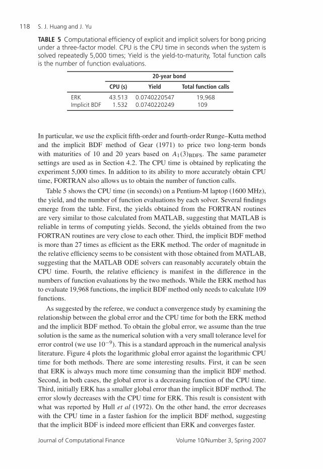
TABLE 5 Computational efficiency of explicit and implicit solvers for bong pricingunder a three-factor model. CPU is the CPU time in seconds when the system issolved repeatedly 5,000 times; Yield is the yield-to-maturity, Total function callsis the number of function evaluations.

20-year bond

CPU (s) Yield Total function calls

ERK 43.513 0.0740220547 19,968Implicit BDF 1.532 0.0740220249 109

In particular, we use the explicit fifth-order and fourth-order Runge–Kutta methodand the implicit BDF method of Gear (1971) to price two long-term bondswith maturities of 10 and 20 years based on A1(3)BDFS. The same parametersettings are used as in Section 4.2. The CPU time is obtained by replicating theexperiment 5,000 times. In addition to its ability to more accurately obtain CPUtime, FORTRAN also allows us to obtain the number of function calls.

Table 5 shows the CPU time (in seconds) on a Pentium-M laptop (1600 MHz),the yield, and the number of function evaluations by each solver. Several findingsemerge from the table. First, the yields obtained from the FORTRAN routinesare very similar to those calculated from MATLAB, suggesting that MATLAB isreliable in terms of computing yields. Second, the yields obtained from the twoFORTRAN routines are very close to each other. Third, the implicit BDF methodis more than 27 times as efficient as the ERK method. The order of magnitude inthe relative efficiency seems to be consistent with those obtained from MATLAB,suggesting that the MATLAB ODE solvers can reasonably accurately obtain theCPU time. Fourth, the relative efficiency is manifest in the difference in thenumbers of function evaluations by the two methods. While the ERK method hasto evaluate 19,968 functions, the implicit BDF method only needs to calculate 109functions.

As suggested by the referee, we conduct a convergence study by examining therelationship between the global error and the CPU time for both the ERK methodand the implicit BDF method. To obtain the global error, we assume than the truesolution is the same as the numerical solution with a very small tolerance level forerror control (we use 10−9). This is a standard approach in the numerical analysisliterature. Figure 4 plots the logarithmic global error against the logarithmic CPUtime for both methods. There are some interesting results. First, it can be seenthat ERK is always much more time consuming than the implicit BDF method.Second, in both cases, the global error is a decreasing function of the CPU time.Third, initially ERK has a smaller global error than the implicit BDF method. Theerror slowly decreases with the CPU time for ERK. This result is consistent withwhat was reported by Hull et al (1972). On the other hand, the error decreaseswith the CPU time in a faster fashion for the implicit BDF method, suggestingthat the implicit BDF is indeed more efficient than ERK and converges faster.



FIGURE 4 The logarithmic global error as a function of the logarithmic CPU timefor both the ERK method and the implicit BDF method.

Logarithmic CPU Time

Loga

rithm

ic G

loba

l Err

or

3.760 3.764 3.768 3.772

-18

-17

-16

-15

-14

-13

-12

Convergence Study for ERK

Logarithmic CPU Time

Loga

rithm

ic G

loba

l Err

or

-0.6 -0.4 -0.2 0.0 0.2 0.4

-18

-17

-16

-15

-14

-13

-12

Convergence Study for BDF

5 CONCLUSIONS AND IMPLICATIONS

Stiffness in ODEs exists widely in the continuous-time finance literature. Thepresence of stiffness causes all of the explicit solvers that have been suggestedand widely used in the literature to be numerically inefficient. The proceduresproposed in the present paper are based on implicit numerical methods whichhave unbounded stability regions, greater flexibility on the choice of the stepsize,and hence lead to improved numerical efficiency.

We apply the implicit methods to price zero-coupon bonds and to estimateaffine dynamic term structure models via ECF under two affine models. We showthat the procedures are highly effective to improve numerical efficiency withoutsacrificing statistical efficiency. As a result, affine models can be much moreefficiently analyzed and hence computationally even more attractive than non-affine models. However, the techniques themselves are quite general and can beapplied in many other contexts. For example, the methods can be used in connec-tion with more efficient ECF procedures for estimation, including the proceduresof Singleton (2001) and Carrasco et al (2006). Since these more efficient ECFprocedures require more intensive numerical calculation of ODEs, one naturallyexpects greater gains in using the implicit methods. Also, the methods extend



naturally to more complicated affine models, including the affine jump-diffusionmodels (Duffie et al (2000); Chacko and Das (2002)) and semi-affine models(Duffee (2002); Duarte (2004)), where greater gains should be expected in theimplicit methods as the dimension of the system grows. Furthermore, the methodscan be applied to specifications outside of the affine family. An example is thequadratic affine model of Ahn et al (2002), where bond prices are shown to bedependent on a system of ODEs, although not Ricatti equations.

We have provided evidence of stiffness in bond markets. However, otherfinancial markets can also have stiff problems. For example, using the estimatesin the two-factor volatility models (termed LL2V, LL2V1, and LL2VF) obtainedby Chernov et al (2003) from stock market data, we obtain the following stiffnessratios: 8,886.6, 1,028.6 and 426.5. These suggest severe stiffness.

Our methods can be applied to price many other financial assets as longas stiffness is a feature in a system. Examples include coupon-bearing bonds,swaptions, captions, mortgage-back securities, bond options, stock options, andcurrency options. As the calculation of these financial instruments is usuallycomputationally more demanding than zero-coupon bonds, there may be furtheradvantages of using the implicit methods over the explicit methods.

The implicit methods examined in the present paper include an implicit Runge–Kutta method and an implicit linear multi-step method. Both methods have theirown merits. To take advantage of the merits of both methods, a new type of hybridmethod, called the implicit general linear method, has appeared in the numericalODE literature in recent years (Butcher (2003); Huang (2005)). How well theimplicit general linear methods perform in financial stiff problems will be reportedlater.

APPENDIX A

When estimating the two-factor CIR model via ECF, the following 30 pointswere used to evaluate the CCF and ECF: (0.01, 0), (0, 0.01), (0.01, 0.01), (0.02,0.01), (0.01, 0.02), (0.02, 0.02), (0.03, 0.02), (0.02, 0.03), (0.03, 0.03), (0.04,0.03), (0.03, 0.04), (0.04, 0.04), (0.04, 0.05), (0.05, 0.04), (0.05, 0.05), (−0.01,0), (0, −0.01), (−0.01, −0.01), (−0.02, −0.01), (−0.01, −0.02), (−0.02, −0.02),(−0.03, −0.02), (−0.02, −0.03), (−0.03, −0.03), (−0.04, −0.03), (−0.03,−0.04), (−0.04, −0.04), (−0.04, −0.05), (−0.05, −0.04), (−0.05, −0.05).

When estimating the three-factor model of Balduzzi et al (1996) via ECF, thefollowing rule is used to select 52 points to evaluate the CCF and ECF. First,ri takes one of the three values 0, 0.01, or 0.02. All possible combinations in(r1, r2, r3), excluding the origin, yield 26 different points. We then take negativevalues of these 26 points to get another 26 points.

REFERENCES

Ahn, D., Dittmar, R. F., and Gallant, A. R. (2002). Quadratic term structure models: theoryand evidence. Review of Financial Studies 15, 243–288.



Aiken, R. C. (1985). Stiff Computation. Oxford University Press, Oxford.

Aït-Sahalia, Y. (2003). Closed-form likelihood expansion for multivariate diffusion.Working Paper, Princeton University.

Aït-Sahalia, Y., and Kimmel, R. (2003). Estimating affine multifactor term structure modelsusing closed-form likelihood expansion. Working Paper, Princeton University.

Balduzzi, P., Das, S., Foresi, S., and Sundaram, R. (1996). A simple approach to three factoraffine term structure models. Journal of Fixed Income 6, 43–53.

Bates, D. (1996). Jumps and stochastic volatility: exchange rate processes implicit in PHLXdeutschmark options. Review of Financial Studies 9, 69–107.

Black, F., and Scholes, M. (1973). The Pricing of Options and Corporate Liabilities. Journalof Political Economy 81, 637–659.

Bogacki, P., and Shampine, L. F. (1989). A 3(2) pair of Runge–Kutta formulas. AppliedMathematics Letters 2, 1–9.

Butcher, J. C. (2003). The Numerical Analysis of Ordinary Differential Equations. John Wiley& Sons, Chichester.

Carrasco, M., Chernov, M., Florens, J., and Ghysels, E. (2006). Efficient estimation ofjump diffusions and general dynamic models with a continuum of moment conditions.Journal of Econometrics, to appear.

Chacko, G., and Das, S. (2002). Pricing interest rate derivatives: a general approach.Review of Financial Studies 15, 195–241.

Chacko, G., and Viceira, L. M. (2003). Spectral GMM estimation of continuous-timeprocesses. Journal of Econometrics 116, 259–292.

Chen, R. R., and Scott, L. (1992). Pricing interest rate options in a two-factor Cox–Ingersoll–Ross model of the term structure. Review of Financial Studies 5, 613–636.

Chen, R. R., and Scott, L. (1993). Maximum likelihood estimation of a multi-factorequilibrium model of the term structure of interest rates. Journal of Fixed Income 3,14–31.

Chernov, M., Gallant, A. R., Ghysels, E., and Tauchen, G. (2003). Alternative models ofstock prices dynamics. Journal of Econometrics 116, 225–257.

Cox, J., Ingersoll, J. and Ross, S. (1985). A Theory of the term structure of interest rates.Econometrica 53, 385–407.

Dahlquist, G. (1963). A special stability problem for linear multistep methods. BIT 3,27–43.

Dahlquist, G. (1985). Some comments on stability and error analysis for stiff non-lineardifferential systems. Stiff Computation, Aiken., R. C. (ed.). Oxford University Press,Oxford.

Dahlquist, G., and Björck, A. (1974). Numerical Methods. Prentice-Hall, Englewood Cliffs,NJ.

Dai, Q., and Singleton, K. J. (2000). Specification analysis of affine term structure models.Journal of Finance 55, 1943–1978.

Dormand, J. R., and Prince, P. J. (1980). A family of embedded Runge–Kutta formulae.Journal of Computational Applied Mathematics 6, 19–26.



Duarte, J. (2004). Evaluating an alternative risk preference in affine term structure models.Review of Financial Studies 17, 379–404.

Duffee, G. R. (2002). Term premia and interest rate forecasts in affine models. Journal ofFinance 57, 405–443.

Duffie, D. (2001). Dynamic Asset Pricing Theory. Princeton University Press, New Jersey.

Duffie, D., and Kan, R. (1996). A yield-factor model of interest rate. Mathematical Finance6, 379–406.

Duffie, D., Pan, J., and Singleton, K. J. (2000). Transform analysis and asset pricing foraffine jump-diffusions. Econometrica 68, 1343–1376.

Engle, R., and Lee, G. (1999). A long-run and short-run component model of stockreturn volatility. Cointegration, Causality and Forecasting, Engle, R. and White, H. (eds).Oxford University Press, Oxford.

Gear, G. W. H. (ed.) (1971). Numerical Initial Value Problems in Ordinary DifferentialEquations. Prentice-Hall, Englewood Cliffs, NJ.

Geyer, A., and Pichler, S. (1999). A state-space approach to estimate and test multifactorCox–Ingersoll–Ross models of the term structure. Journal of Financial Research 22,107–130.

Heston, S. L. (1993). A closed-form solution for options with stochastic volatility, withapplication to bond and currency options. Review of Financial Studies 6, 327–343.

Huang, S. J. (2005). Implementation of general linear methods for stiff ordinary differentialequations. PhD Thesis, Department of Mathematics, University of Auckland.

Hull, T. E., Enright, W. E., Fellen, B. M., and Sedgwick, A. E. (1972). Comparing numericalmethods for ordinary differential equations. SIAM Journal of Numerical Analysis 9,603–637.

Iserles, A. (1996). A First Course in the Numerical Analysis of Differential Equations.Cambridge University Press, Cambridge.

Jagannathan, R., Kaplin, A., and Sun, S. (2003). An evaluation of multi-factor CIR modelsusing LIBOR, swap rates, and cap and swaption prices. Journal of Econometrics 116,113–146.

Klopfenstein, R. W. (1971). Numerical differential formulas for stiff systems of ordinarydifferential equations. RCA Review 32, 447–462.

Lo, A. W. (1988). Maximum likelihood estimation of generalized Itô processes withdiscretely sampled data. Econometric Theory 4, 231–247.

Phillips, P. C. B., and Yu, J. (2005). Jackknifing bond option prices. Review of FinancialStudies 18, 707–742.

Piazzesi, M. (2003). Affine term structure models. Handbook of Financial Econometrics,to appear.

Shampine, L. F., and Reichelt, M. W. (1997). The MATLAB ODE suite. SIAM Journal ofScientific Computing 18, 1–22.

Singleton, K. J. (2001). Estimation of affine asset pricing models using the empiricalcharacteristic function. Journal of Econometrics 102, 111–141.



Vasicek, O. (1977). An equilibrium characterization of the term structure. Journal ofFinancial Economics 5, 177–186.

Yu, J. (1998). The empirical characteristic function in time-series estimation. PhD Thesis,Department of Economics, University of Western Ontario.

Yu, J. (2004). Empirical characteristic function estimation and its applications. EconometricReviews 23, 93–123.

Zedan, H. (1990). Avoiding the exactness of the Jacobian matrix in Rosenbrock formulae.Computers and Mathematics with Applications 19, 83–89.


Date post:	11-Feb-2022
Category:	Documents
Upload:	others
View:	9 times
Download:	0 times

On stiffness in affine asset pricing models - Singapore Management

Documents