ehavior is examined using the retarded-motion expansion coefficients of bead-spring chains at different levels of coarse-graining.how the trade-off between using too few or too many springs. The general framework to analyze the force–extension and rheologics applied to the worm-like chain, FENE, and Fraenkel models. We introduce a new method for coarse-graining a polymer into a bhain called the Polymer Ensemble Transformation (PET) method. Application to the freely jointed chain polymer yields a set of spaws called the Random Walk Spring (RWS) model. This new method illustrates why the previous spring force-laws cannot be useiscretize polymers and also provides new insight into how to rationally proceed in the coarse-graining of polymers into bead-spr2004 Elsevier B.V. All rights reserved.
Polymers are challenging to model due to the wide range ofime and length scales in the system. A recurring theme in theevelopment of polymer models and simulations is the ideaf coarse-graining. The goal in coarse-graining is to producemodel that has reduced complexity such that it is tractable
o calculate the properties of the model while simultaneouslyapturing molecular properties to sufficient accuracy.
Some of the earliest attempts at coarse-graining polymersonsisted of eliminating degrees of freedom for whichhere are only small fluctuations, such as bond lengthsnd bond angles. This led to models including the freely
ointed chain (FJC) in which each bond is treated as a freeoint and the freely rotating chain (FRC)[1]. A much moreuccessful model which includes hindered rotation is the
rotational isomeric state (RIS) model[2]. While RIS hasbeen successful in determining the equilibrium propertiepolymers, understanding the dynamics of polymers reqthe use of a coarser model.
One example of a coarser model is a FJC in whichlength of a step is taken to be larger than a bond[3]. Inthis model the length of a rod, or Kuhn length, represthe length over which the polymer acts as if the swere uncorrelated. This model represents a chain thcoarse-grained to the length of a Kuhn length. One gadvantage of this model is that the distribution functionconfigurations is well-known from the theory of randwalks. It should be noted that there is a difference betwthe random walk distribution and the bead-rod chainrigid constraints[4]. This latter model with rigid constrainwill be referred to solely as the Kramers chain in this paThe former model, with a distribution function identito the random walk, will be referred to as either the frejointed chain or random walk chain.
Using this knowledge of the distribution function it hasbeen shown that the FJC has an elastic restoring force thatis linear for small deformations, and is given by the inverseLangevin function over the entire range of deformations[3].Although other polymer models, such as the worm-like chain(WLC), have a different form for the restoring force, thiselasticity is one of the main properties of polymers that dis-tinguishes them from small molecules and thus must be cap-tured in a coarse-grained model. The restoring force is pri-marily due to the entropy of the polymer so it is often re-ferred to as the “entropic restoring force”. When develop-ing a coarse-grained polymer model, the fine details of thepolymer configurations must necessarily be lost. These “mi-crostates” contribute significantly to the entropy, and thus tothe elastic restoring force. Something else must be added tothe system that represents this restoring force without repre-senting all the “microstates”. This restoring force has oftenbeen represented by springs, thus modelling the polymer asa bead-spring chain.
While much work has been performed using Hookeansprings, it is well known that finite-extensibility plays animportant role in determining the rheological properties ofpolymers[4–7]. For that reason, this paper will focus pri-marily on springs that have a finite fully extended length.However, within this class of springs, there exists a wide va-r ew -e tot ed tionst ,f itera-t or thes ationo
dy-n ains,a eteri lic-i ins.L att ngesa foundt h fortt ide-l Fur-t haven ificialc ere hab ay toi db tl ther ringc
Understanding the behavior of bead-spring chains, in par-ticular under what conditions they represent accurate coarse-grained models, is becoming increasingly important in thestudy of polymers. Previous studies have suggested that bead-spring chains only accurately represent polymers when eachspring represents a large segment of polymer. The study byLarson et al. suggests that springs can only model the WLC ifeach spring represents a large number of persistence lengths.Similarly, Somasi et al.[14] have argued based on the force–extension behavior of the Kramers chain[19] that springs canonly represent a Kramers chain if each spring represents morethan 10 Kuhn lengths. Thus from force–extension behavior itwould seem that a single spring (or dumbbell) model wouldbest represent a polymer.
However, some rheological considerations require the op-posite extreme, that the polymer is modelled by as manysprings as computationally tractable. The behavior of a poly-mer in flow is highly dependent on the drag exerted onthe polymer by the solvent. In a bead-spring chain model,the drag is exerted on the chain only at the beads. Thusthe drag will only be exerted along a continuous contourin the limit of a large number of springs. The rheologicalbehavior of a polymer is also dependent on its distributionof relaxation times. To capture this distribution, the bead-spring model must have a large number of modes, and thusa fs ly-m onlyb ymera -e oneo mbero lle
por-t d thec merb r oft ead-s vior.W s tol niand ught e-c nicala niand r canb turea di-m seriese rge ors
cant hasb ior tor logy.
iety of forms for the spring force-law[8]. These include thorm-like chain model[9,10], the finitely extensible nonlinar elastic (FENE) model[11], and other approximations
he inverse Langevin function[12]. Note that in this paper wo not consider any of the numerous closure approxima
hat have been proposed in the literature[5,13]. Furthermoreor each of the models there are discrepancies in the lure as to the “best” parameters that should be chosen fpring force-law in order to have an accurate representf the polymer behavior[14–16].
Most of these previous studies have used Brownianamics to examine the rheological properties of the chnd then used some procedure to determine the param
n the model. In fact only a few studies have looked exptly at the force–extension behavior of bead-spring chaarson et al.[17,18]showed using Brownian dynamics th
he force–extension behavior of a bead-spring chain chas more and more beads are added to the chain. They
hat a parameter in the force-law (the persistence lengthe case of the WLC model) could beartificially changedo obtain better results from the model. However, no guines have been given for the use of such a method.hermore, the conditions under which the method failsot been quantified, and the consequences of the arthange have not been evaluated. For these reasons, theen variability between investigators as to the best w
mplement the correction, or evenif the correction shoule used. To answer important questionsincluding but noimited to these, one must analyze in a systematic wayamifications of coarse-graining a polymer into bead-sphains.
s
s
large number of springs[4]. Finally, the large number oprings may be motivated primarily by geometry. If a poer is placed in a confining geometry, its behavior cane described correctly if the model represents the polt a small enough length scale[20–22]. The task of modlling a polymer accurately using bead-spring chains isf balancing these two opposing considerations. The nuf springs must besimultaneouslylarge enough and smanough.
The force–extension behavior is of fundamental imance to the understanding of bead-spring chains anhoice of force-law. The very idea of replacing the polyy springs is motivated by the force–extension behavio
he polymer. Thus we begin our systematic study of bpring chains by analyzing their force–extension behahile other investigators have used Brownian dynamic
ook at the force–extension behavior, we use both Browynamics and equilibrium statistical mechanics. Altho
he methods giveidenticalresults, equilibrium statistical mhanics has major advantages. The statistical mechanalysis avoids the stochastic noise intrinsic in Browynamics simulations so the force–extension behavioe calculated quickly and accurately. The analytic nalso allows for the easy identification of the importantensionless parameters, as well as the construction of
xpansions when those parameters become either lamall.
After understanding the force–extension behavior weurn to the study of rheological properties, applying whateen learned. The first step from force–extension behavheology is examining zero Weissenberg number rheo
This is because in zero Weissenberg number flow, a polymerhas sufficient time to sample all of phase space. To examinethis limit, the retarded-motion expansion coefficients of thebead-spring chain can be examined.
This paper is organized as follows. InSection 2the twomethods used, equilibrium statistical mechanics and Brown-ian dynamics, are reviewed briefly.Section 3contains an ex-tensive analysis of the force–extension behavior of the bead-spring chains. This includes a discussion of the correction-factor employed by Larson et al.[18], a discussion of thefluctuations about the mean extension, and a discussion ofuniversal behavior.Section 4examines the rheological be-havior of the bead-spring chains in the limit of zero Weis-senberg number by examining the first two coefficients ofthe retarded-motion expansion. InSection 5the analysis inthe previous sections is shown to be generally valid for anychoice of force-law by showing explicitly how the analysiswould be performed for two other important models. The twoexamples given are the FENE force-law and the infinitelystiff Fraenkel force-law (equivalent to the FJC).Section 6introduces a new method for choosing the spring force-law called the Polymer Ensemble Transformation (PET)method. We apply this method to the FJC to calculate aspring force thatexactlymatches the force–extension be-havior of the FJC called the Random Walk Spring (RWS)m thep -e arliers
2
ls ofc s thatw ow-n
2
forw lied.W thep to[
e
i on-si re.T ont oftenu qualt
Given the above definition, the probability density at theconfigurationi, pi, is given by
pi = 1
Zexp
[−Heff,i
kBT
](2)
whereZ is the partition function and is equal to
Z =∫
· · ·∫
configurationsexp
[−Heff
kBT
]dV (3)
to ensure that the probability density is properly normalized.It should be noted that for the bead-spring chains consideredin this paper we do not need to worry about the kinetic energycontribution to the effective Hamiltonian and the momentumconfiguration space[4]. This is because our system has norigid constraints that freeze-out degrees of freedom, and alsowe will not compute the average of any quantity that dependson momentum.
Average quantities are computed by integrating that quan-tity times the probability density over all the configurationspace. Thus for a property signified byF the average is
〈F 〉 =∫
· · ·∫
configurationsF
1
Zexp
[−Heff
kBT
]dV (4)
2
b qui-l larbi usedB e an-a findi ane andp oft Thisw
met mer.T
m
w d,rd ,t h thev duet beadi e willn hus,
F
odel. Not only does this new model perform better thanrevious models, the method illustrateswhy the other modls perform in the manner discussed throughout the eections.
. Methodology
The behavior of bead-spring chains at different leveoarse-graining has been investigated using two methodill be reviewed briefly here, statistical mechanics and Brian dynamics.
.1. Statistical mechanics
In this paper we will only be discussing systemshich equilibrium statistical mechanics can be appithin this context of equilibrium statistical mechanics
robability density of a configuration is proportional23]
xp
[−Heff
kBT
](1)
f the configuration is consistent with the macroscopic ctraints. The quantityHeff is the effective Hamiltonian,kB
s Boltzmann’s constant, andT is the absolute temperatuhe specific form of the effective Hamiltonian depends
he macroscopic constraints, i.e. the ensemble. For thesed canonical ensemble the effective Hamiltonian is e
o the energy.
.2. Brownian dynamics
The technique of Brownian dynamics (BD)[24,25] haseen widely used to study the non-equilibrium and e
ibrium properties of polymer models in flow, in particuead-rod and bead-spring models[19,26,27]. Most previous
nvestigations of the behavior of bead-spring chains haveD. Because the systems studied in this paper can all blyzed using equilibrium statistical mechanics also, we
t natural to use that methodology. In order to providexplicit link between the statistical mechanical resultsrevious work using BD, we will perform BD simulations
he force–extension behavior of the bead-spring chains.ill verify that the two methods giveidenticalresults.The method of BD consists of integrating forward in ti
he equation of motion for each of the beads in the polyhe equation of motion is given by
i r i = Fnet,i = FB,i + Fd,i + Fs,i 0 (5)
here the subscripti denotes beadi,m the mass of each bea¨ the acceleration,Fnet the net force,FB the Brownian forceue to collisions of the solvent molecules with the beadsFd
he drag force due to the movement of each bead througiscous solvent, andFs the systematic force on each beado the springs and any external forces. The drag on eachs taken to be the Stokesian drag on a sphere, and weglect any hydrodynamic interaction between beads. T
whereζ is the drag coefficient, andu∞(r i) is the undisturbedsolvent velocity evaluated at the center of beadi. The gov-erning stochastic differential equation then becomes
r i(t) u∞(r i(t)) + 1
ζ[Fs,i(r j(t)) + FB,i(t)] (7)
The Brownian force is chosen from a random distributionsuch that it has the following expectation values:
〈FB,i(t) 〉 = 0 (8)
〈FB,i(t)FB,j(t) 〉 = 2kBTζδij
δtδ (9)
The symbolδij is the Kronecker delta,δ the unit second-order tensor, andδt the time-step. These expectation val-ues are needed so that the system satisfies the fluctuation-dissipation theorem. The stochastic differential equation canbe re-written as
r i(t) u∞(r i(t)) + 1
ζFs,i(r j(t)) +
√2kBT
ζ δtdWi (10)
whereWi is a Wiener process that satisfies
〈dWi〉 = 0 (11)
〈dWi dWj〉 = δij δ (12)
licitfi
r
I ainsw fort me,t ianf fullye aper,t t noe ourseo
ionb
t
w er.T thena
t
T
δ
wheref is the externally applied force. Variance reduction[24] was also employed to reduce the stochastic noise at smallforce.
3. Force–extension behavior
As was mentioned in the introduction, one of the mostimportant and widely known properties of polymers is elas-ticity, and in particular the presence of an “entropic restoringforce”. Furthermore, with the advent of optical and magnetictweezer technologies, much more attention is being paid tothe relation between force and extension[28]. In particular,these experiments have been used to test polymer modelswhich are then used in other contexts.Making quantitativecalculations of the force–extension behavior of bead-springchains for comparison with the polymers they represent is thegoal of this section.
3.1. System definition
The typical set-up used to calculate the restoring force us-ing statistical mechanics is shown inFig. 1. One end of thepolymer is tethered at the origin, and a constant external force,f , is applied to the other end of the polymer. The direction oft es nep e oft c-t ep is isd ysiss eldfi rta nsi mpu-t rreda ains,af
F forcee e freee to
In the work presented here we will use a simple exprst-order time-stepping algorithm:
i(t + δt) r i(t) + r i(t) δt (13)
t should be noted that when simulating bead-spring chith finitely extensible springs with the above criteria
he Brownian force and an explicit time-stepping schehere can be a small but finite probability that the Brownorce will cause a spring to be stretched beyond thextended length. In the simulations presented in this phe time-stepδt was always taken small enough such thaxamples of over-stretching were observed over the cf the simulation time.
In the BD simulation performed of the force–extensehavior, the system was equilibrated for
eq = 4 × 10³
(ζA2
true
kBT
)(14)
hereAtrue is the true persistence length of the polymhez-position of the end of the bead-spring chain wasveraged for
ave = 8 × 10³
(ζA2
true
kBT
)(15)
he time-step used was
t = 4 × 10⁻³(ζAtrue
f
)(16)
his constant force defines thez-direction of the coordinatystem. Thex andy coordinates are therefore in the plaerpendicular to the applied force. The expectation valu
he polymer’szdisplacement,〈z〉, can be calculated as a funion of the applied force. This function,〈z〉 vs.f , defines tholymer’s force–extension (F–E) behavior. Note that thifferent from the behavior found by performing the analhown inFig. 2, in which the ends of the polymer are hxed at points that arez (or equivalentlyr) distance apand the average force,〈f 〉, to hold them at those positio
s calculated. Because the former approach is more coationally tractable than the latter, it has been the prefepproach by previous investigators using bead-spring chnd it will be the approach initially used here. SeeSection 6
or a more detailed comparison of the two approaches.
ig. 1. Illustration of a polymer and bead-spring model in the constantnsemble. One end is held fixed, while a constant force is applied to thnd. The direction of the force defines thez-direction. Thez-displacemenf the chain is averaged.
Fig. 2. Illustration of a polymer and bead-spring model in the constant ex-tension ensemble. Both ends are held fixed at a distancer apart. The externalforce required to hold one of the ends fixed is averaged.
When developing a bead-spring model for the polymer,it is crucial to verify that the model accurately describes thepolymer. Because the concept of replacing the polymer by abead-spring chain is largely motivated by the F–E behavior, itseems natural to verify the accuracy of the coarse-graining byrequiring that the F–E behavior of the bead-spring chain is thesame as the polymer it represents. However, it is also criticalthat the bead-spring chain is compared to the polymer usingthe exact same “experiment”. Since the polymer behavior iscalculated by applying a constant force, as shown inFig. 1,the bead-spring behavior will be calculated in the same way.
3.2. Decoupled springs
Because the bead-spring model is in the (Np)fT ensem-ble (the number of polymersNp is trivially held constant atone), the effective Hamiltonian is obtained by performinga Legendre Transform fromz to f [23]. Thus the effectiveHamiltonian is
Heff = U − fztot (17)
whereU is the potential energy of the bead-spring system(recall that all kinetic energy has been dropped), andztot thez-coordinate of the end of the chain. For all the systems con-s po-t d ont t thee eachs
H
w fe ring,a eH pring,tp
Z
whereNs is the number of springs in the chain, andZs isgiven by
Zs =∫
exp
[−Us(r) + fz
kBT
]d3r (20)
This separation of the partition function has two importantconsequences. First, the computational effort needed to cal-culate the F–E behavior is greatly reduced because the prop-erties of any size chain can be determined by knowing theproperties of asingle spring(a single integral). Second, it il-lustrates that for this set of conditions the springs are decou-pled. In particular, it will be shown later that the F–E behaviorof these bead-spring chain models does not depend explicitlyon the number of beads, which act as free hinges, but onlydepends on the level of coarse-graining for each spring. Thisis counter to other investigators who have argued the impor-tance of the number of springs in the bead-spring chain model[18].
3.3. Dimensionless parameters
In describing the behavior of bead-spring chains it is usefulto define a set of dimensionless variables. Many of these vari-able transformations are motivated by the worm-like chain(WLC) force-law, which is the force-law that correctly de-s ma-t ma-t tb ownl heirp -l
z
λ
we tho thepr encel pre-s ergyf l,U as ac onlesse
U
I pro-pt entedb
idered here, the potential energy will have no bendingentials, and the energy for each spring will only depenhe magnitude of extension. It should then be clear thaffective Hamiltonian can be separated into a sum overpring
eff =∑j
[Us(rj) − fzj] (18)
herej denotes each spring,Us(rj) the potential energy oach spring as a function of the radial extension of the spndzj thez-displacement of springj. Because the effectivamiltonian can be decomposed into a sum over each s
he partition function for the whole chain,Zw, splits into aroduct of the partition functions for single springs,Zs,
w = (Zs)Ns (19)
cribes the behavior of dsDNA. Specifically the transforions are motivated by the interpolation formula approxiion to the WLC by Marko and Siggia[10]. However, it muse noted that the formula remain general, as will be sh
ater inSection 5. A summary of these parameters and thysical interpretations is given inTable 1. These dimension
ess variables are
ˆtot ≡ ztot
L, r ≡ r
, f ≡ fAtrue
kBT, α ≡ L
Atrue,
≡ Aeff
Atrue, ν ≡ α
Ns=
Atrue(21)
hereL is the contour length of the chain, ≡ L/Ns the fullyxtended length of a spring,Atrue the true persistence lengf the polymer,α the number of true persistence lengths inolymer’s contour,Aeff the effective persistence length,λ theatio of the effective persistence length to the true persistength, andν the number of true persistence lengths reented by each spring. It is also useful to define two enunctions. First, we will denote asUeff (r) the spring potentia
s(r), with all additive constants dropped. This is doneonvenience and changes no results. Second, a dimensinergy is defined as
ˆ eff (r) = Ueff (r)
kBT
λ
ν(22)
t will become clear later that this scaling is the one apriate for the spring potential, in which it is scaled bykBT
imes the number of effective persistence lengths represy each spring.
LTotal z-displacement as fraction of contour length
rr
Radial single spring displacement as fraction of fully extended length
ffAtrue
kBTExternally applied force in units ofkBT divided by true persistence length
αL
AtrueNumber of true persistence lengths in polymer’s contour length
λAeff
AtrueEffective persistence length in units of the true persistence length
ν
AtrueNumber of true persistence lengths represented by each spring
Ueff (r)Ueff (r)
kBT
λ
νPotential energy of a spring in units ofkBT times the number of effective persistence lengths represented by each spring
3.4. Force–extension results
The F–E behavior is now calculated using a general resultbased onEqs. (3), (4), and (17):
〈ztot〉 = kBT∂
∂flnZ (23)
For bead-spring chains in particular, for whichZ→ Zw, us-ing Eq. (19)and non-dimensionalizing withEq. (21)showsthat
〈ztot〉m = 1
ν
∂
∂flnZs (24)
where the m-subscript on the mean fractional extension isused to signify that it is for the bead-spring model. The angu-lar integration for the single spring partition function can beperformed, resulting in the following formula for the meanfractional extension:
〈ztot〉m = 1
ν
−1
f+ ∂
∂fln
(∫ 1
0dr r sinh[νf r]
× exp
[−ν
λUeff (r)
])(25)
T deldo erwb ngb
theM tedt eent tionf lledb e”W ndS vior
is given by[10]
f = 〈ztot〉p − 1
4+ 1
4(1− 〈ztot〉p)2(26)
where the p-subscript on the mean fractional extension sig-nifies that it is the exact value for the polymer (to separate itfrom the behavior of the bead-spring model). It has been con-ventional for this behavior to directly motivate the followingchoice for the spring force-law:
fspring(r) =(kBT
Aeff
)( r
)− 1
4+ 1
4(1− r/)2
(27)
It should be emphasized that thisassumptionhas replaced themean fractionalz-projection of the polymer with the frac-tional radial extension of the spring. The true persistencelength appearing in the polymer behavior has also been re-placed by the effective persistence length in the spring force-law to use as a “correction-factor”. Integrating the springforce-law gives the effective spring potential
Ueff (r) = kBT
(
Aeff
)1
2
( r
)2 − 1
4
( r
)+ 1
4(1− r/)
(28)
which results in a dimensionless energy of
U
bothE e-g arkoa -a qualst nd ringf lsou thel
odelc ength
his shows explicitly that the F–E behavior of the moepends parametrically only onν andλ, but not explicitlyn the number of springs,Ns. This means that a polymith α = 400 represented by 40 springs has anidenticalF–Eehavior as a polymer withα = 10 represented by 1 spriecause both haveν = 10.
At this point it is useful to apply these definitions toarko and Siggia interpolation formula. It should be no
hat within the context of this paper the differences betwhe interpolation formula and the exact numerical soluor the WLC are unimportant. Thus the polymer modey our so-called WLC model is not quantitatively the “truLC, but is a hypothetical polymer for which the Marko aiggia formula is exact. For this polymer, the F–E beha
ˆ eff (r) = r2
2− r
4+ 1
4(1− r)(29)
Specific examples of F–E behavior, calculated usingq. (25)and BD, can be seen inFig. 3as the level of coarsraining,ν, is changed. The spring potential used is the Mnd Siggia interpolation formula (Eq. (29)), and for all exmples in the figure the effective persistence length e
he true persistence length (λ = 1). Most of the Browniaynamics simulations were performed using a single sp
or simplicity. However, we calculate one of the points asing 20 springs to explicitly show dependence only on
evel of coarse-graining,ν.The fact that the F–E curve for a bead-spring m
hanges as more springs are added for a fixed contour l
Fig. 3. Calculation of the relative error of the mean fractional extension,(〈ztot〉m − 〈ztot〉p)/〈ztot〉p, for a bead-spring model as the level of coarse-graining changes. The Marko and Siggia potential was used withλ = 1. Thecurves correspond toν = 400 (dashed),ν = 20 (dotted), andν = 10 (dash-dot). The symbols represent Brownian dynamics simulations. The singlespring simulations correspond toν = 400 (), ν = 20 (), andν = 10 ().The twenty-spring simulation corresponds toν = 10 (•). Inset: The meanfractional extension of the models compared with the “true polymer” (solidline, Eq. (26)).
has been seen before[18]. However, the conventional expla-nation for this discrepancy is that the introduction of moresprings directly introduces extra flexibility, which pulls inthe end of chain resulting in a shorter extension for the sameforce. FromEq. (25)we see that this cannot be fully cor-rect because the absolute number of springs never appearsonly the level of discretization of each spring.Thus the force–extension curve of a bead-spring chain under any conditionscan be understood by only considering the behavior of a sin-gle spring, and how its force–extension behavior changes asthe number of persistence lengths it represents changes.
3.5. Phase space visualization
To get a better physical understanding of why the F–Ebehavior deviates from the polymer, let us examine the prob-ability density function over the configuration space. In gen-eral for a bead-spring chain the phase space has too manydimensions to visualize easily. However as we just saw theF–E behavior can be understood by looking at a single spring,which has a phase space of only three dimensions.
Recall that the probability density is proportional to
exp
[−Heff
kBT
](30)
s fec-t Theca
H
For the case of a single spring as considered here the effectiveHamiltonian is
Heff = Ueff (r) − fz = kBTν
(Ueff (r)
λ− f z
)(32)
and therefore the important configurations are determined by
Heff ≡(Ueff (r)
λ− f z
)=
(Ueff (r)
λ− f z
)min
+ O
(1
ν
)
(33)
where we have defined a dimensionless effective Hamilto-nian,Heff . FromEq. (33)we see that 1/ν plays a similar rolein the F–E behavior as temperature usually does in statis-tical mechanics, determining the magnitude of fluctuationsin phase space about the minimum. A detailed and quan-titative description of fluctuations will be performed laterin Section 3.7. Here we will discuss how the portion ofphase space the system samples (fluctuates into) with signif-icant probability determines the mean extension. In the limitν → ∞, the system is “frozen-out” into the state of minimumHeff . Note that asν → ∞, the polymer becomes infinitelylong. By calculating thefractionalextension, we are scalingall lengths by the contour length. Thus even though the fluc-tuations may not be getting small if a different length scalew ns oft con-t se onale o.
sf ngp eso alld n-t ee-dac alueso eo um-b pleswc -idi truep thes tedw hemi -e hy asν s thet -
o that only configurations near the minimum of the efive Hamiltonian contribute significantly to the average.onfigurations that contribute must have aHeff less thankBT
bove the minimum:
eff = (Heff )min + O(kBT ) (31)
,
ere used (such as the radius of gyration), the fluctuatiohe end-to-end distance do go to zero compared to theour length. Alternatively in the limitν → 0, the system iqually likely to be in any state, and thus the mean fractixtension of the bead-spring chain,〈ztot〉m, approaches zer
In order to understand the behavior at intermediateν,Fig. 4hows a contour plot ofHeff for the four casesf = 0.444,ˆ = 5,λ = 1, andλ = 1.5, and the Marko and Siggia spriotential(Eq. (29)). The contour lines correspond to linf constantHeff within the x–z plane. Note that becauseirections perpendicular to ˆz are equivalent, rotating the co
our lines about the ˆz axis produces surfaces in the thrimensional phase space with constantHeff . While Heff ,nd therefore the contour plots, are independent ofν, theyan be used to understand the behavior at different vf ν because ofEq. (33). The value ofν governs the sizf the fluctuations around the minimum, and thus the ner of contour lines above the minimum the system samith significant probability. We also see that each of theHeffontours is not symmetric about the minimum ofHeff , causng the mean extension of the bead-spring chain,〈ztot〉m, toeviate from the point of minimumHeff . Forλ = 1 the min-
mum of Heff corresponds to the mean extension of theolymer,〈ztot〉p. This is because of the way of choosingpring potential from the true polymer behavior as illustraith Eqs. (26)–(29). As λ is increased, the position of tinimum moves to larger ˆz while the depth of the minimum
ncreases. The minimum also moves to larger ˆz and deepns when the force is increased. These plots explain w→ ∞ the bead-spring chain behavior only approache
rue polymer behavior ifλ = 1, why asν → 0 the mean frac
Fig. 4. Visualization of phase space using contours of constantHeff for asingle spring with the Marko and Siggia potential. The square () representsthe position of the “true polymer” mean fractional extension,〈ztot〉p. Thecross (×) represents the position of minimumHeff . Upper left:f = 0.444,λ = 1; lower left: f = 0.444, λ = 1.5; upper right:f = 5, λ = 1; lowerright: f = 5, λ = 1.5.
tional extension approaches zero, and why for intermediateν there may exist a value ofλ for which the mean fractionalextension matches the true polymer.
3.6. Correcting the force–extension behavior
Now that we understand better the reasons why the F–Ecurve deviates from the true polymer F–E curve, we wouldlike to change the model to get closer agreement. A very simple method that has been used by previous investigators[18]is to use a different persistence length in the spring force-law(Aeff ) from the true persistence length of the polymer (Atrue),i.e.λ = 1. In particular, ifλ is increased, the extension of thechain also increases, back to the extension of the true polymer. The conventional explanation for this is that the freehinges in the bead-spring chain have introduced extra flexi-bility. To counter-act the flexibility introduced by the hinges,the stiffness of the springs must be increased by increasinthe effective persistence length. Let us now analyze the effect of increasingλ within the framework presented above.Looking atEq. (25)shows that increasingλ acts to decreasethe spring potential energy. Because the spring gets weake(less stiff), it is not surprising that the extension gets larger.It should be noted that for infinitely long polymers increas-ing the persistence length causes a decrease in the restorinf
-s er, id alue
of λ such that the F–E curve exactly matches the true curve.It is unclear what value ofλ to choose to give the “best fit”between the model curve and the true curve. We will presenthere an analysis of possible choices and place bounds on therange of choices. The first criterion that might come to mindis some type of integrated sum of squared error. However,that quantity becomes very cumbersome to manipulate ana-lytically and it is unclear that it is any better of a criterion thananother. The criteria that we will consider looks at matchingexactly one section of the F–E curve. The three sections are atzero applied force, at infinite applied force, and at the appliedforce for which the true polymer has a mean fractional exten-sion of 0.5. Before calculations can be made of the “best-fit”λ in each region, the exact meaning of matching the true poly-mer behavior must be specified. The half-extension criterionis straight-forward: we will require that the model and poly-mer curves are equal at the point where the polymer is at halfextension. The other two criteria are more subtle because themodel and polymer become equal at zero and infinite forcefor all values ofλ. For the low-force criterion we will requirethat the slopes of the F–E curves be equal at zero force. Itshould be noted that this is equivalent to requiring that therelative error of the model goes to zero at zero force. Again,a similar criterion cannot be used at infinite force becausethe slope (or relative error) will always be zero at infinity
atniterac-finitet-C
lsowntted).ings,hence
orce.Though it is true that by increasingλ from one the exten
ion increases towards the true extension of the polymoes so non-uniformly. This means that there exists no v
-
-
g-
r
g
t
independent ofλ. Thus our infinite force criteria will be ththe relative error of the slope of the F–E curve at infiforce will equal zero. Physically, this means that the ftional extension versus force curves approach one at inforce in the same manner.Fig. 5 shows a plot of the “besfit” λ versus 1/ν for each of the three criteria for the WLforce-law.
Fig. 5. Calculation ofλ for the three different criteria at different leveof coarse-graining for the Marko and Siggia potential. The criteria share low-force (dash-dot), half-extension (dashed), and high-force (doUpper axis: the level of coarse-graining in terms of the number of sprNs, for a polymer withα = 400 (approximatelyλ-phage DNA stained witYOYO at 4 bp:1 dye molecule). Inset: expanded view showing the divergof the criteria.
It is important to mention that both the low-force and half-extension curves diverge for a finite 1/ν. This means thatthere exists aν small enough such that the low-force or half-extension region cannot be matched simply by adjustingλ.The position of these divergences can be calculatedexactlyin a simple manner as will be shown inSection 3.8. For theWLC the low-force curve diverges atν∗ = 10/3 while thehalf-extension curve diverges atν∗ = 2.4827. However thehigh-force curve is alwaysλ = 1 for finite 1/ν.
To illustrate the difference between the three choices ofλ, let us look at a specific example.Fig. 6shows the relativeerror in the mean fractional extension versus force for theWLC force-law, three different values ofλ, andν = 20. Thethree values ofλ correspond to the three criteria shown inFig. 5. By comparing the relative error curves, we can seethe entire range of effectsλ has on the F–E behavior. Thecriteria at low and high force form a bound on the choicesfor a “best-fit”λ as seen inFig. 6, even if none of the criteriapresented here is believed best.
As a further example we show the parameters that wouldbe chosen to modelλ-phage DNA at different levels ofcoarse-graining, as well as some properties of the models.These parameters could be used in a Brownian dynamicssimulation to capture the non-equilibrium properties ofλ-phage DNA.Tables 2–4show what effective persistence
Models with 10, 20, and 40 springs are compared using three best-fitλ criteriaAtrue = 0.053 m, andα = 352.8.
Fig. 6. Calculation of the relative error of the mean fractional extension,(〈ztot〉m − 〈ztot〉p)/〈ztot〉p, for a bead-spring model for different best fit crite-ria. The Marko and Siggia potential was used withν = 20. The curves cor-respond toλ = 1.41 (low-force, dotted),λ = 1.21 (half-extension, dashed),andλ = 1 (high-force, dash-dot). Inset: the mean fractional extension of themodels compared with the “true polymer” (solid line,Eq. (26)).
ing properties of the model were calculated from formulaein Section 4. The contour length and persistence length forunstainedλ-phage DNA were taken from Bustamante et al.[29]. We used that the contour length is increased by 4A perbis-intercalated YOYO dye molecule[30], and we assumed
−0.0010 0.0208 −0.0013 0.023
−0.0010 0.020−0.00073 0.017
6 −0.0013 0.022−0.00091 0.019
length to choose for the model for the different “best-fit” cteria and for different staining ratios of dye. The paramewere calculated by repeated application ofFig. 5. The result-
Table 2Table of properties for models of unstainedλ-phage DNA
Models with 10, 20, and 40 springs are compared using three best-fitλ criteria. 4 bp:1 dyeλ-phage DNA has the following properties:L = 21.1 m,Atrue = 0.053m, andα = 398.1.
that the persistence length of the stained molecule is thesame as the unstained value.
In these tables we see examples of the expected generaltrends. As the polymer is more finely discretized, the num-ber of persistence lengths represented by each spring,ν, de-creases. This causes a larger spread in the possible choicesfor the effective persistence length, and thus a larger spreadin properties. We see the general trend that the magnitudeof the properties decreases asν decreases. Note that for thelow-force criterion,Rg andη0,p are exactly the “Rouse re-sult”. The “Rouse Result” is the value of the Rouse model ifthe spring constant is taken to be the zero-extension slope ofthespringforce-law. The “Rouse result” will be discussed inmore detail inSection 4. The only difference from the “truepolymer” is that the mass and drag are localized at the beadsinstead of along a continuous contour. This is true untilν
reaches the point of divergence of the low-force criterion.However,b2 andτ0 are only approximately the “Rouse re-sult” as discussed inSection 4. The properties for the otherbest-fit criteria have even smaller magnitude than the low-force criterion. This decrease is due to an error in the zero-force slope of the force–extension curve, and thus a smallercoil size.
3.7. Fluctuations
el, iti n ex-t s far.I usb heF un-d ainst in afl ucho inest ar-t oft l role[
It is shown inAppendix A that the fluctuations can becalculated as
(δz)2 = 〈(ztot − 〈ztot〉m)2〉m = 1
Nsν
∂
∂f〈ztot〉m
= 1
α
∂
∂f〈ztot〉m (34)
(δx)2 = 〈(xtot)2〉m = 〈(ytot)
2〉m = 1
Nsν f〈ztot〉m
= 1
α f〈ztot〉m (35)
where we have defined the root-mean-squared fluctuations asδzandδx. One important thing to notice about the fluctuationsis that once the F–E behavior is known (〈ztot〉m versusf ), thefluctuations can be calculated directly without performingany further integrations. In fact, both types of fluctuations canbe calculated by finding the slope of a line on the F–E curve,as seen inFig. 7. From the figure we see that the longitudinalfluctuations are proportional to the slope of the curve, whilethe lateral fluctuations are proportional to the slope of the lineconnecting the point of the F–E curve to the origin. Becausethe F–E curve is concave,the lateral fluctuations are alwaysgreater than or equal to the longitudinal fluctuations.
fl thec el ofc ectedst poly-m merl vari-a blesi ymerc -s owedt nsb inso only
In addition to discussing the F–E behavior of the mods important to discuss the fluctuations around the meaension. We have already seen the use of fluctuations thun Section 3.5we saw how examining fluctuations can helpetter understand themeanextension. The fluctuations in t–E behavior are also important in trying to extend ourerstanding from the F–E behavior of the bead-spring ch
o the behavior in a flow field. For a bead-spring chainow field, the fluctuations of the chain determine how mf the flow field the chain can sample. In turn this determ
he total force applied to the chain by the flow. This is picularly important in shear flow, in which the fluctuationhe chain in the shear gradient direction plays a centra8,31].
Another important aspect ofEqs. (34) and (35)is that theuctuations depend explicitly on the number of springs inhain, unlike the F–E curve which just depends on the levoarse-graining for each spring. In fact we see the expcaling of the root-mean-squared fluctuations asα−1/2. Sincehe persistence length is the length-scale over which theer backbone loses correlation, the fluctuation of the poly
ength should scale like a sum of “independent” randombles. The number of these “independent” random varia
s precisely the number of persistence lengths in the polontour,α. We show inFigs. 8 and 9plots of the root-meanquared fluctuations for the same cases for which we shhe F–E behavior inFig. 3. We have scaled the fluctuatioyα1/2 to collapse the fluctuations of different length chanto the same curve. The fluctuations after this scaling
Fig. 7. Graphical illustration of longitudinal and transverse fluctuations. Fora given forcef , the longitudinal fluctuations are proportional to the slopeof the tangent curve (dashed). The transverse fluctuations are proportionalto the slope of the chord (dotted) connecting the origin to the point on theforce–extension curve.
depend on the number of persistence lengths represented byeach spring,ν, and the ratio of the effective persistence lengthto the true persistence length,λ.
Note that it is easy to calculate exactly the high-force scal-ings for the fluctuations usingEqs. (34) and (35)and ourknowledge of the high-force scaling for〈ztot〉m. It is easy toshow that for bead-spring chains using the Marko and Siggiapotential (Eq. (29)) the high-force scaling is
〈ztot〉mf→∞∼ 1 − 1
2λ1/2f1/2
+ O
(1
f
)(36)
F ns atd usedw dν ptotic
b
Fig. 9. Calculation of the transverse root-mean-squared fluctuations at dif-ferent levels of coarse-graining. The Marko and Siggia potential was usedwithλ = 1. The curves correspond toν = 400 (dashed),ν = 20 (dotted), andν = 10 (dash-dot). The solid line corresponds to the high-force asymptotic
behavior, 1/(f1/2
).
Using this result, we can show that
α1/2 δzf→∞∼ 1
2λ1/4f3/4
+ O
(1
f5/4
)(37)
α1/2 δxf→∞∼ 1
f1/2
+ O
(1
f
)(38)
Of particular interest are the fluctuations at “equilibrium”(zero applied force) because it relates to the size of the poly-mer coil. In the context of the F–E behavior, that is equivalentto calculating the slope of the F–E curve at zero force, as canbe seen by taking the limitf → 0 in Eqs. (34) or (35). Bytaking that limit, and rewriting the average as the average ofthe radial coordinate of a single spring, it can be shown that
limf→0
(∂
∂f〈ztot〉m
)= ν
3
∫ 10 dr r4 exp[−(ν/λ) Ueff (r)]∫ 10 dr r2 exp[−(ν/λ) Ueff (r)]
(39)
This expression was used previously inSection 3.6to calcu-late the “best-fit”λ at zero force as seen inFig. 5, and it willbe used extensively to understand rheological properties inSection 4.
We also note here that Ladoux and Doyle[31] derived anexpression similar toEq. (35)based on scaling argumentsand a single spring. Based on the scaling argument, they de-v ntald
3
pringc r ar-b ina-t e theb ation
ig. 8. Calculation of the longitudinal root-mean-squared fluctuatioifferent levels of coarse-graining. The Marko and Siggia potential wasithλ = 1. The curves correspond toν = 400 (dashed),ν = 20 (dotted), an= 10 (dash-dot). The solid line corresponds to the high-force asym
ehavior, 1/(2f3/4
).
eloped a model which compared favorably to experimeata and lends support to the results presented here.
.8. Limiting behavior (asymptotic expansions)
We have seen thus far that the F–E behavior of bead-shains can be written analytically as integral formulae foitrary spring force-law. This has allowed for the determ
ion of the important dimensionless groups that determinehavior, as well as provide for rapid and accurate calcul
through numerical integration. However, another importantadvantage to having analytical formulae is that expansionscan be performed. Those expansions can be used to illustratelimiting and universal behavior as well as obtain approxi-mate algebraic formulae that illustrate what aspects of theforce-law are needed to estimate the exact behavior withoutperforming numerical integration.
We have already seen numerically inFig. 3 that the F–E behavior of the model only matches the “true” polymerbehavior if each spring represents a large number of per-sistence lengths. Thus it seems natural to find asymptoticexpansions of the integrals in the limitν → +∞. We startby expanding directly the force–extension curve (Eq. (25)).The asymptotic expansion is a straightforward application ofLaplace’s Method[32]. The calculation is made significantlyeasier by noting that the hyperbolic sine can be replaced byonly the growing exponential, because it only results in sub-dominant corrections. Up to first order, the expansion is givenby
〈ztot〉mν→∞∼ c + 1
ν
[−1
f+ 1
c
(∂c
∂f
)+ (∂2c/∂f
2)
2(∂c/∂f )
]
+ O
(1
ν2
)(40)
w
c
W -i mer.H func-t nm inedf theWe vioro icali
0
Tt ctf ntialwa e tos tP
rs . Ift icef F–Ec gEe me
Fig. 10. Comparison of the fractional extension with its highν asymptoticexpansion for the Marko and Siggia potential withλ = 1 andf = 0.1. Thecurves correspond to the exact result (solid line), the expansion includingO(1/ν) (dotted), and the zero-one PadeP0
1 (1/ν) (dashed). Inset: the analo-gous comparison forf = 1.25.
if and only if the spring force-law is an odd function of itsargument (the potential is an even function).
Even for the case of an odd spring force-law, it is morecomputationally convenient to obtain the expansion of theslope of the F–E curve at zero force directly by expandingEq.(39). Application of Laplace’s Method requires the expansionof the spring force-law, of the following form:
Ueff (r) = φ0 + φ2r2 + r3
∞∑i=0
hiri (43)
Note that there is no linear term because we require this po-tential to look Hookean near ˆr = 0 and that the value of theconstant term,φ0, does not affect the final answer. Also notethatφ2 > 0.
Proceeding with Laplace’s Method, the complete asymp-totic series can be calculated to be the following:
limf→0
(∂
∂f〈ztot〉m
)ν→+∞∼
(λ
2φ2
)×
∞∑i=0
di
(λ
ν φ2
)i/2
(44)
The coefficients of the series can be calculated from a collec-tion of recursion relations that include the coefficients of theTaylor series of the spring potential. The recursion relationsare given here for completeness:
d
d
here
≡ 〈ztot〉p(λf ) (41)
e thus see again that asν → ∞ with λ = 1 the F–E behavor of the bead-spring model approaches the true polyowever, we also have the correction terms written as a
ion of thetrue polymerF–E curve.No assumptionhas beeade about the spring force-law other than it is determ
rom the “true polymer” F–E behavior as was done forLC model inSection 3.4. Provided the value ofν is “large
nough”,Eq. (40)can be used to estimate the F–E behaf a bead-spring model without performing any numer
ntegrations for any value off or λ within
< f < ∞, 0 < λ < ∞ (42)
o give a sense of the applicability of the expansion inEq. (40)o smallerν, we show inFig. 10a comparison of the exaorce–extension result for the Marko and Siggia poteith λ = 1 and the asymptotic expansion for forcesf = 0.1nd f = 1.25. We see that the expansion is applicablmallerν whenf is larger. The zero-one Pade approximan01(1/ν) is seen to improve the smallν behavior.
Care must be taken ifEq. (40)is expanded for large omall f because of the order in which limits are takenhe F–E curve is expanded to O(ν−a), then the asymptotxpansionf → ∞ can only be obtained to O(f
−a). At low
orce, the quantity of greatest interest is the slope of theurve at zero force, given byEq. (39). In general, expandinq. (39)directly for ν → ∞ gives a different result fromxpandingEq. (40)for smallf . The expansions are the sa
We have also examined the ability to use this expansion atsmallerν, as shown inFig. 11 for the Marko and Siggiapotential withλ = 1. It should be noted that the zero-onePade P0
1(1/ν1/2) performs worse than the first two termsof the expansion inEq. (44). However, the two-point zero-two Pade P0
2(1/ν1/2) that includes the behavior at smallν does perform better. This lowν behavior will now bediscussed.
In addition to examining the bead-spring chains in thelimit ν → ∞, it is interesting to examine the F–E behavior inthe limit ν → 0. In this limit the F–E behavior can approacha curveindependentof the functional form ofUeff (r). Phys-ically one can think of this limit as taking a polymer withfixed contour length, and infinitely discretizing the model.Therefore each spring is becoming very small. However, itshould also be noted that each spring is getting weaker, asseen inEq. (32). It has been postulated previously that asthe chain is infinitely discretized, the F–E behavior wouldapproach that of the freely jointed chain[18]. Using the for-malism presented thus far, we can examine explicitly thislimit and test the postulated behavior. To understand the F–Ebehavior in this limit, we simply need to expandEq. (25)forν → 0.
It should first be noted that expanding the prescribed in-tegral is an example of an integral that can only be expanded
Fig. 11. Comparison of the zero-force slope with its highν asymptotic ex-pansion for the Marko and Siggia potential withλ = 1. The curves cor-respond to the exact result (solid line), the expansion including O(1/ν1/2)(dotted), the zero-one PadeP0
1 (1/ν1/2) (dashed), and the two-point zero-twoPadeP0
2 (1/ν1/2) (dash-dot).
rigorously using asymptotic matching, but the leading-orderbehavior is relatively easy to obtain[32]. In fact, the leadingorder behavior is obtained by setting
exp
[−ν
λUeff (r)
] 1 (48)
By further expanding the hyperbolic sine, it can be easilyshown that
〈ztot〉mν→0∼ νf
5, f fixed (49)
Note that this is consistent withSection 3.5in which we sawthat, for f fixed, the mean fractional extension approacheszero asν → 0. We also see explicitly that the F–E behaviordoes notapproach the FJC, which is given by
〈ztot〉m = L(f ) (50)
where
L(x) = coth(x) − 1
x(51)
is the Langevin function. We can also contrast the behavior inEq. (49)with a different “experiment” in which free hingesato freeh aver-aa
〈
ep del isi inep stemi ever,a ldingf era Onem roleo hisc noc(
〈
W am
〈
re introduced into a truecontinuousworm-like chain whilehe force is held constant. If one considersν to be the ratiof the contour length of the continuous curve betweeninges to the persistence length, then it is clear that thege extension of this discretized worm-like chain,〈ztot〉dwlc,pproaches the limit
ztot〉dwlcν→0∼ L(νf )
ν→0∼ 13(νf ), f fixed (52)
It should be noted that holdingf fixed corresponds to thhysical process of holding the force constant as the mo
nfinitely discretized. This is the appropriate limit to examrocesses in which the force applied to the end of the sy
s independent of how the system is discretized. Hownother universal result can be obtained by instead of hoˆ fixed, holdingνf fixed. This corresponds to pulling hardnd harder on the model as it is more finely discretized.ight expect that the length of a spring should play thef the “Kuhn length”, and thus the scale for the force. Torresponds to a dimensionless force ofνf . The expansiof the bead-spring chain model behavior withνf fixed isalculated by simply integrating the hyperbolic sine inEq.25) to obtain
ztot〉mν→0∼ −3
νf+ 1
L(νf ), (νf ) fixed (53)
e see that even in this limit the systemdoes notapproachodified “freely jointed chain” result of
To understand the true limiting shape (Eq. (53)) it can beshown that
−3
x+ 1
L(x)≈ L
(x
2
), x large (55)
−3
x+ 1
L(x)≈ L
(3x
5
), x small (56)
In addition to being used to understand the limit of infinitediscretization,Eq. (53)can be used to understand the diver-gence of the “best-fit”λ curves inFig. 5 and discussed inSection 3.6. Recall that previously we considered the limit inEq. (53)to be asν → 0 as (νf ) was held fixed, andλ was im-plicitly being held constant. By examiningEq. (25), we seethat if (νf ) is held constant, the only remaining parameter isν/λ. Thus the expression inEq. (53)can be rewritten as thelimit (ν/λ) → 0:
〈ztot〉mλ→∞∼ −3
νf+ 1
L(νf ), bothν, f fixed (57)
Now suppose that one is choosingλ such that the modelmatches the true polymer at an extension of〈ztot〉p, whichoccurs at a force denotedf (〈ztot〉p). The value ofν for whichthat “best-fit” curve diverges (denotedν∗) will be the valuefor which only asλ → ∞ will the extension of the modelequal that of the polymer. This condition is written as
〈
T orcec yo r, itc
〈
I
T ia is
ν
B wws lf-e -s enb
w
0 ria,
in general itcannotbe used for the high force criteria. Thisstems from the break-down of the assumption inEq. (48)if f → ∞, in particular because the spring potential for theWLC model diverges at full extension fast enough. In fact,we know thatEq. (58)cannot be valid for the WLC modelfor the high-force criterion because we know that the highforce criteria does not diverge. It is shown inSection 5.1that the high force criteria for the FENE model does di-verge, andEq. (58)canbe used to calculate the position ofdivergence.
4. Rheological properties
Thus far we have only considered the force–extensionbehavior of the bead-spring chains. In addition to F–E be-havior we are interested in the rheology of the bead-springchains, and how it changes as the level of coarse-grainingchanges. In general, this is a much harder problem com-putationally than the work done thus far. In order to con-tinue in the spirit of calculating properties near equilibriumand using equilibrium statistical mechanics, we will investi-gate the rheology of the bead-spring chains by looking atpotential flow in the limit of small deformation rate. Po-tential flow has the desirable property that the chain behav-i nicsw ysist lated.T per-t ingfl
ded-m Thish earE eta ded-m ow-e sim-p andi cifica insb sly,w be-t s ont lecta eent ilute.W ientsc thef ivenb
〈
ztot〉p = −3
ν∗f (〈ztot〉p)+ 1
L(ν∗f (〈ztot〉p))(58)
his can also be used to find the divergence of the low friteria by examining the limit asf → 0. Because of the waf choosing the force-law from the true polymer behavioan be shown easily that
ztot〉pf→0∼ f
2φ2(59)
t can also be shown that
−3
ν∗f (〈ztot〉p)+ 1
L(ν∗f (〈ztot〉p))
f→0∼ ν∗f5
(60)
herefore the point of divergence for the low force criter
∗ = 5
2φ2(61)
y applying Eq. (61) to the Marko and Siggia force-lae see that the low force criteria diverges atν∗ = 10/3 astated inSection 3.6. To calculate the divergence for the haxtension criteria, we set〈ztot〉p = 1/2 in Eq. (58)and subtitute forf (1/2) fromEq. (26). The divergence is then givy the solution to
1
2= −3
5ν∗/4+ 1
L(5ν∗/4)(62)
hich isν∗ = 2.4827 as stated inSection 3.6.It must be noted that whileEq. (58) is valid for any< 〈ztot〉p < 1, and can be used for the low force crite
or can be calculated using equilibrium statistical mechaith an effective energy due to the flow. From this anal
he retarded-motion expansion coefficients can be calcuhese coefficients give insight into the rheological pro
ies of the bead-spring chains in slow and slowly varyows.
Thus the goal of this section is to examine the retarotion expansion coefficients for bead-spring chains.as been done previously for Finitely Extensible Non-linlastic (FENE)[5] springs and for Hookean springs. Birdl. [4] also present a general framework for the retarotion coefficients for any bead-spring-rod chain. H
ver, because of the generality, that analysis cannotlify the integrals over phase space to a convenient
ntuitive form. Here we present the results of a spepplication of that framework to only bead-spring chaut for arbitrary spring force-law. As assumed previoue will assume that there are no bending potentials
ween springs and that the spring force only dependhe magnitude of extension. Furthermore we will negny hydrodynamic interaction and excluded volume betw
he beads and assume that the polymer solution is dith these assumptions, the retarded-motion coeffic
an be written as a function of simple moments oforce-law probability distribution. These moments are gy
Written in terms of the moments, the first two retarded-motion expansion coefficients equal
b1 − ηs = η0,p = 136npζ(N2 − 1)〈r2〉eq (64)
b2 = −Ψ1,0
2
=(
−npζ2
120kBT
)[(〈r4〉eq
15− 〈r2〉2
eq
9
)(N4 − 1
N
)
+( 〈r2〉2
eq
9
)((N2 − 1)(2N2 + 7)
6
)](65)
where ηs is the viscosity of the Newtonian solvent,η0,pthe polymer contribution to the zero-shear viscosity,Ψ1,0the zero-shear first normal stress coefficient,np the numberdensity of polymers,ζ the drag coefficient of each bead,andN the number of beads in the chain. Because we haveneglected hydrodynamic interaction, we also know fromBird et al. [4] that b11 is zero. SeeAppendix B for thederivation of these coefficients. It should be emphasized thatfor Eqs. (64) and (65)no assumptionhas been made aboutthe form of the spring force-lawUeff (r).
A more common approach to calculating the polymer con-tribution to the zero-shear viscosity is through the Giesekusform of the stress tensor, from which it can be shown that
η
w qui-l les
R
F ,a op-el latedf
τ
Rt letF
〈
A ded-m
b
b2 = −Ψ1,0
2=
(−np(Nζ)2L2A2
true
120kBT
)
×(
ν2〈r4〉eq
15− ν2〈r2〉2
eq
9
)((N2 + 1)(N + 1)
N3(N − 1)
)
+(ν〈r2〉eq
3
)2 ((N + 1)(2N2 + 7)
6N2(N − 1)
) (71)
The advantage of working with the dimensionless momentsis that they only depend on the parametersν andλ but not onthe absolute number of beads (or springs). Thus all depen-dence on the absolute number of beads is shown explicitly.In this way we have separated out in the formulae the con-tribution from the specific form of the spring force-law andthe contribution from the chain having multiple beads. Con-trary to the force–extension behavior, we do see a dependenceon the absolute number of beads. The coefficients are madedimensionless as
η0,p = η0,p
np(Nζ)LAtrue/12(72)
b2 = b2 (73)
nd onlyo ofs berd -m ngthA areu in isN
s es iff , wer lec
otionc entsd thel -s ds,N eη sc -iafi da odelt ymer,t in thel sit e
0,p = 16npζNR2
g (66)
hereRg is the root mean square radius of gyration at eibrium. For bead-spring chainsRg is related to the singpring moments as
2g = N2 − 1
6N〈r2〉eq (67)
rom these equations we can verifyEq. (64). Eqs. (64), (65)nd (67)were additionally used to calculate the model prrties given inTables 2–4as discussed inSection 3.6. A re-
axation time for the bead-spring chain can also be calcurom the retarded-motion expansion coefficients:
0 = −b2
b1 − ηs(68)
ecalling from the definitions of the moments (Eq. (63)) thathey are defined for asingle spring, it seems natural to scahem by the fully extended length of a spring,, if it is finite.or that case let us define dimensionless moments as
rn〉eq = 〈rn〉eq
n=
∫ 10 dr rn+2 exp[−(ν/λ)Ueff (r)]∫ 1
0 dr r2 exp[−ν/λUeff (r)](69)
fter a number of parameter substitutions the retarotion expansion coefficients can be rewritten as
1 − ηs = η0,p =(np(Nζ)LAtrue
12
)(N + 1
N
)(ν〈r2〉eq
3
)
(70)
−np(Nζ)2L2A2true/(120kBT )
These were chosen as the scales because they depen properties intrinsic to the true polymer or the systemtudy. The polymer solution being modelled has a numensity of polymers,np, and a temperatureT . The true polyer being modelled has a value of the persistence letrue, a contour lengthL, and a total drag. Because wesing a freely draining model, the total drag on the chaζ. By comparing dimensionless quantities withNζ as thecale of drag, we are looking at how the property changor bead-spring models with different number of beadsecalculate the drag on a single bead,ζ, such that the whohain has a constant drag.
To better understand the behavior of the retarded-moefficients, let us first examine how much the coefficiepend explicitly on the number of beads (in addition to
evel of coarse-graining,ν). In Figs. 12 and 13we show repectivelyη0,p andb2 as a function of the number of bea, while the level of coarse-graining,ν, is held constant. Th
ˆ0,p curves for different values ofν are exactly self-similar aould be seen fromEq. (70), while theb2 curves are approxmately self-similar except when bothν andN are small. Wettribute the change of the coefficients withN while ν is heldxed to the fact that for finiteN the drag is not distributelong a continuous contour. Thus for the bead-spring m
o be an accurate coarse-grained model of the true polhe number of beads must be large enough to operateargeN region. The deviation forν < ∞ is due to the errorn the spring force-law as discussed inSection 3with regardso the F–E behavior. Theν = ∞ curve corresponds to th
Fig. 12. Polymer contribution to the zero-shear viscosity of Marko andSiggia bead-spring chains as the number of effective persistence lengthsrepresented by each spring,ν/λ, is held constant. The curves correspondto ν/λ = ∞ (solid line), ν/λ = 400 (dotted),ν/λ = 100 (dashed), andν/λ = 10 (dash-dot).
“Rouse model” result. What we mean by the “Rouse model”result will be discussed later.
In order to model a given polymer with different numbersof beads, the value ofν is not constant. Instead the value ofα (the number of true persistence lengths in the polymer’scontour) is constant. InFigs. 14 and 15we show respectivelyη0,p andb2 as a function of the number of beads,N, whileα
is held constant. This corresponds to discretizing a polymerfiner and finer. We can see the interplay between drag errorand discretizing error as discussed in the introduction. Whenthe number of beads is small, error is present because the dragon the polymer due to the solvent is lumped at the beads,not exerted along a continuous contour. When the numberof beads is large, error is present because the polymer hasbeen discretized so finely that each spring represents a smallnumber of persistence lengths. As discussed previously this
F bead-s nted byel
Fig. 14. Polymer contribution to the zero-shear viscosity of Marko and Sig-gia bead-spring chains as the number of effective persistence lengths inthe total polymer contour,α/λ, is held constant. The curves correspondto α/λ = ∞ (solid line), α/λ = 4000 (dotted),α/λ = 400 (dashed), andα/λ = 100 (dash-dot).
fine discretization leads to error predicting the size of thecoil and the extension of polymer segments. If the number ofpersistence lengths in the whole polymer,α, is large enough,there exists an approximate plateau. This corresponds to thesituation in which the number of springs is simultaneouslylarge enough to reduce the drag error and small enough toprevent discretization error. Using the expansions developedin Section 3.8we canpredictthe location of this plateau.
To use these expansions and also explain why the behaviorapproaches the “Rouse result”, we need to express the springmoments in terms of the force–extension behavior. FromEq.(39)we see that
limf→0
(∂
∂f〈ztot〉m
)= ν〈r2〉eq
3(74)
F bead-s totalp∞(
ig. 13. Zero-shear first normal stress coefficient of Marko and Siggiapring chains as the number of effective persistence lengths represeach spring,ν/λ, is held constant. The curves correspond toν/λ = ∞ (solid
ig. 15. Zero-shear first normal stress coefficient of Marko and Siggiapring chains as the number of effective persistence lengths in theolymer contour,α/λ, is held constant. The curves correspond toα/λ =
It can also be shown by taking the third derivative of theforce–extension curve that
1
3νlimf→0
(∂3
∂f3〈ztot〉m
)= ν2〈r4〉eq
15− ν2〈r2〉2
eq
9(75)
Making use of these equalities we can write the retarded-motion expansion coefficients as
η0,p =(N + 1
N
)(limf→0
∂
∂f〈ztot〉m
)(76)
b2 = 1
3νlimf→0
∂3
∂f3〈ztot〉m
(
(N2 + 1)(N + 1)
N3(N − 1)
)
+(
limf→0
∂
∂f〈ztot〉m
)2 ((N + 1)(2N2 + 7)
6N2(N − 1)
) (77)
Let us first examine the plateau of ˆη0,p. We can easily see fromthe pre-factor inEq. (76)that the drag error is negligible if
N 1 (78)
To predict the upper limit of the plateau, we use the expansionin Eq. (44). Use of this series is justified because we knowtv ant.F
|
W tw
(
N theM
φ
HT
(
w -cf
1
b lect
the term with the third derivative. Following an analogousprocedure we find the plateau region forb2:
2 N, (N − 1)i/2 1
|2di|(αφ2
λ
)i/2
(84)
Note the factors of two that result from expanding the rationalfunction ofN for largeN and from expanding the square ofthe zero-force slope.
Let us consider application of these formulae to the WLCmodel. For the Marko and Siggia potential withλ = 1 thetwo plateau conditions state that
1 N, (N − 1)1/2 1.151α1/2 (85)
2 N, (N − 1)1/2 0.576α1/2 (86)
If we consider that an order of magnitude difference is suf-ficient to satisfy the conditions, then the conditions couldbe approximated as
15 N 0.01α (87)
In words this says that the number of beads must be larger thanapproximately 15 while simultaneously each spring must rep-resent more than approximately 100 persistence lengths. Re-call that based on force–extension simulations[19] of theKramers chain, Somasi et al.[14] argued than each springs nota andh LCr to de-r s fora u-l le alid-i is oft
re-g vea n oft lt”.T ouldg nsionsl v-i effi-c
η
b
W f themr ap-p
hat if the behavior is within the plateau region thenν must beery large. In fact, the leading order term must be dominor the WLC model this corresponds to
d1|(
λ
νφ2
)1/2
1 (79)
ritten in terms of the parameterα/λ, which is constanhile discretizing, this condition becomes
N − 1)1/2 1
|d1|(αφ2
λ
)1/2
(80)
ote that this is true for the WLC model because forarko and Siggia spring potential
2 = 3
4, d1 = −4
3√π
(81)
owever some models like the FENE model haved1 = 0.he appropriate analysis shows that in general
N − 1)i/2 1
|di|(αφ2
λ
)i/2
(82)
herei denotes the first coefficientdi that is non-zero (exluding d0 = 1). Combining the two bounds onN gives aormula for the plateau region for ˆη0,p:
N, (N − 1)i/2 1
|di|(αφ2
λ
)i/2
(83)
A similar analysis can be done forb2. Becauseα has toe large for a plateau region to even exist, we will neg
hould represent more than 10 Kuhn lengths but wereble to estimate a lower bound on the number of springsad to extrapolate from the Kramers chain result to the Wesult. Here we have used zero Weissenberg rheologyivebothlower and upper bounds on the number of beadrbitrary spring force-law. From Brownian dynamics sim
ations of start-up of steady shear flow[14], there is initiavidence that our bounds may even retain approximate v
ty in unsteady, strong flows. We leave a detailed analyshis to future research.
In addition to allowing for the derivation of the plateauion, writingb1 andb2 in terms of the force–extension curllows for a better physical understanding for the deviatio
he curves forν < ∞and what is meant by the “Rouse resuhe “Rouse result” is the value that the Rouse model wive if the spring constant were equated to the zero-extelope of thespringforce-law. Recalling that thespringforce-aw was taken from thetrue polymerforce–extension behaor, one can show that this Rouse model would have coients
ˆ0,p =(N + 1
N
)(limf→0
∂
∂f〈ztot〉p
)(88)
ˆ2 =(
limf→0
∂
∂f〈ztot〉p
)2 ((N + 1)(2N2 + 7)
6N2(N − 1)
) (89)
e see that because the force–extension behavior oodel approaches that of the true polymer asν → ∞, the
etarded-motion expansion coefficients of the modelroach the Rouse result. Note that while the part ofb2 with the
third derivative is zero for the Rouse result because its springis Hookean, that term vanishes for the model asν → ∞ be-cause of the 1/ν pre-factor. The third derivative of the truepolymer force–extension curve isnotzero.
Now we turn to a discussion of how using a best-fitλ
criteria affects the rheological behavior as the polymer ismore finely discretized. In particular let us look more closelyat the low-force criteria. The low-force criteria is such that
limf→0
∂
∂f〈ztot〉m = lim
f→0
∂
∂f〈ztot〉p (90)
If we put this result intoEqs. (76) and (77)we see thatthe zero-shear viscosity equals the Rouse result exactly. Thezero-shear first normal stress coefficient will be close to theRouse result but will deviate slightly. This is because thethird derivative is non-zero andν is not infinite. Note thatthe third derivative is also not equal to the third derivativeof the true polymer force–extension curve. The equality andapproximate equality with the Rouse results holds only up toa criticalN, at which point the low-force criterion diverges(Eq. (61)):
Nmax = 25φ2α + 1 (91)
5. Examples of other force-laws
eenn beenu orkf hef awsc
5
e-l vioro bew
f
I n totia
H
C hef -mA leart dfl e
“persistence length”. For the FJC the generalized flexibilitylength is proportional to the Kuhn length.
To apply the framework presented inSection 3 tothe FENE force-law inEq. (92), we will let Atrue =kBT/(Htrue) = aK,true/3 so that the “exact” polymer F–Ebehavior is
f = 〈ztot〉p
1 − 〈ztot〉2p
(94)
This directly motivates the choice for the spring force-law
fspring(r) =(kBT
Aeff
)r/
1 − (r/)2(95)
whereAeff is defined in the expected way as
Aeff = kBT
Heff = aK,eff
3(96)
It is then clear that the dimensionless energy for the FENEspring becomes
Ueff (r) = −1
2ln(1 − r2) (97)
and all formulae fromSection 3follow directly. However,while interpreting the previous discussion it must be kept inmh g ont con-c bilityl rt
te-g F–Eb
〈
w d,o ly int ons:
〈
F
〈
I largeb m-m theF
f
Thus far whenever a particular spring force-law has beeded the Marko and Siggia interpolation formula hassed. It has been noted that the general formula will w
or other force laws. Here we will explicitly show how tormulae can be made specific for two important force-lommonly used in modelling polymer rheology.
.1. FENE force-law
The first force-law we will consider is the FENE forcaw, which is a widely used approximation to the behaf a freely jointed chain (FJC). The FENE force-law canritten in general as
= H〈ztot〉p
1 − 〈ztot〉2p
(92)
n the sense that the FENE force-law is an approximatiohe true force-law for a FJC, the spring constantH is givenn terms of the length of a rod in the FJC, or Kuhn lengthaK,s[4]
= 3kBT
aK(93)
ombiningEqs. (92) and (93), the appropriate scale for torce iskBT/aK, or for the general caseH. The general foralism presented earlier scaled the force bykBT/Atruewheretrue was called the true persistence length. Now it is c
hat it would be more appropriate to callAtrue a generalizeexibility length, and only for the WLC is it equal to th
ind that the parameters dependent onAeff andAtrue canave slightly different physical interpretations dependin
he exact force-law used. What does not change is theept that those parameters consist of generalized flexiengths. Thus, for example,ν still must be large in order fohe bead-spring model to behave like the true polymer.
For the FENE force-law many of the calculations (inrals) can be performed analytically. In particular, theehavior is
ztot〉m = Ik+1(f ν)
Ik(f ν), k = 3 + ν/λ
2(98)
hereIk(x) is the modified Bessel function of the first kinrderk. The moments can also be calculated analytical
erms of the Beta function, or equivalently Gamma functi
rn〉eq = Γ ((n + 3)/2)
Γ (3/2)
Γ (3/2 + ν/(2λ) + 1)
Γ (((n + 3)/2) + ν/(2λ) + 1)(99)
or even values ofn ≥ 2, they take an even simpler form:
rn〉eq = (n + 1)(n − 1) · · · (3)
(n + 3 + ν/λ)(n + 1 + ν/λ) · · · (5 + ν/λ)(100)
n order to more easily compare these results with theody of literature on FENE springs, we will relate the coon FENE notation to the notation used here. TypicallyENE force-law is written as[4]
ComparingEqs. (95) and (101)we see the following equali-ties in notation:
Q → r (102)
Qo → (103)
Hlit → Heff (104)
The other very important parameter in the FENE notation isb defined by
b = HlitQ2o
kBT(105)
which can be related to our notation as
b → ν
λ(106)
For comparison with the WLC results presented thus far,we here present the corresponding results for the FENEmodel. InFig. 16we show the F–E behavior of FENE bead-spring chains as the level of coarse-graining,ν, is changed.We see that the FENE result is qualitatively similar to theWLC result inFig. 3.
For the FENE force-lawλ can also be taken greater thanone to obtain a better behavior from the model.Fig. 17showsthe “best-fit”λ versus 1/ν for each of the three criteria intro-duced inSection 3.6. The most obvious difference from theWLC result inFig. 5is that for the FENE chain the high-forcecriterion curve deviates fromλ = 1. In fact, the high-forcecriterion curve diverges similar to the other criteria. We willsee that this high-force divergence is because of the weakerdivergence of the FENE force-law approaching full exten-sion compared to the WLC force-law. This divergence of thehigh-force criteria also causes the best fitλ curves to form arelatively narrow strip bounding the choices forλ. In Fig. 18
Fig. 16. Calculation of the relative error of the mean fractional extension,(〈ztot〉m − 〈ztot〉p)/〈ztot〉p, for a bead-spring model as the level of coarse-graining changes. The FENE potential was used withλ = 1. The curvescorrespond toν = 400 (dashed),ν = 20 (dotted), andν = 10 (dash-dot).Inset: the mean fractional extension of the models compared with the “truepolymer” (solid line,Eq. (94)).
Fig. 17. Calculation ofλ for the three different criteria at different levelsof coarse-graining for the FENE potential. The criteria shown are low-force(dash-dot), half-extension (dashed), and high-force (dotted). Inset: Expandedview showing the divergence of the criteria.
we compare the force–extension behavior of the three cri-teria for ν = 20. While we see a qualitative match for therelative error with the Marko and Siggia result (Fig. 6), theerror is greatly reduced. Thus for the FENE force-law simplyadjusting the effective flexibility length does a much betterjob at reproducing the true polymer behavior over the entireforce range. This is due to the form of the high-extensiondivergence of the force-law. The trade-off for this improvedperformance is that the range inν that this correction-factorcan be used is reduced.
The high-force and low-force best-fitλ curves can be cal-culated exactly. Recall that the low-force criterion is that theslope at zero force matches the true polymer slope. UsingEq. (39)for the slope, and usingEq. (100)for the second
F ten-s estfi -s ),a on oft
ig. 18. Calculation of the relative error of the mean fractional exion, (〈ztot〉m − 〈ztot〉p)/〈ztot〉p, for a bead-spring model for different bt criteria. The FENE potential was used withν = 20. The curves correpond toλ = 1.33 (low-force, dotted),λ = 1.30 (half-extension, dashedndλ = 1.25 (high-force, dash-dot). Inset: the mean fractional extensi
he models compared with the “true polymer” (solid line,Eq. (94)).
moment, we find that the low-force criteria curve is given by
λ = 1
1 − 5/ν(107)
from which it is easy to see the curve diverges atν∗ = 5.This could also have been seen from the general low-forcedivergence formula inEq. (61)sinceφ2 = 1/2 for the FENEforce-law. The high-force curve is calculated from the high-force expansion of the fractional extension:
〈ztot〉mf→∞∼ 1 − ν/λ + 4
2νf+ O
(1
f2
)(108)
Since the true polymer has a high-force expansion of
〈ztot〉pf→∞∼ 1 − 1
2f+ O
(1
f2
)(109)
the high-force criteria curve is given by
λ = 1
1 − 4/ν(110)
with a divergence atν∗ = 4. This can also be derived fromthe general divergence criteria inEq. (58). By comparing theexpansion
w thatt nd
wwe
s inS edr rse-g NEf eh
α
α
Wt -lawi n oft da f thez can
Fig. 19. Calculation of the longitudinal root-mean-squared fluctuations atdifferent levels of coarse-graining. The FENE potential was used withλ =1. The curves correspond toν = 400 (dashed),ν = 20 (dotted), andν =10 (dash-dot). Inset: detailed look at the high-force limit with solid linescorresponding to the asymptotic behavior, ((ν/λ + 4)/(2ν))1/2(1/f ).
be calculated exactly. Using the expression for the secondmoment of the FENE force-law,
limf→0
(∂
∂f〈ztot〉m
)= ν
5 + ν/λ(115)
We see that the expansion of this slope for largeν should justbe the Taylor expansion. Calculating the coefficients,di, us-ing the FENE force-law shows this explicitly. The parametersof the FENE force-law are
φ2 = 12 (116)
F at dif-fT( ehav-
i
−3
ν∗f (〈ztot〉p)+ 1
L(ν∗f (〈ztot〉p)
f→∞∼ 1 − 2
ν∗f(111)
ith the expansion of the true polymer, we can verifyhe high-force criteria diverges atν∗ = 4. The half-extensioivergence is found by solving the equation
1
2= −3
2ν∗/3+ 1
L(2ν∗/3)(112)
hich has a solutionν∗ = 4.6551.In addition to the F–E behavior of the FENE chains,
hould look at the fluctuations, as done for the WLCection 3.7. In Figs. 19 and 20we show the plots of the scal
oot-mean-squared fluctuations for different levels of coaraining, ν. From the high-force expansion of the FE
orce–extension behavior inEq. (108)we can calculate thigh-force scaling of the fluctuations:
1/2 δzf→∞∼
(ν/λ + 4
2ν
)1/2 1
f+ O
(1
f2
)(113)
1/2 δxf→∞∼ 1
f1/2
+ O
(1
f3/2
)(114)
e can also analyze the limiting behavior fromSection 3.8inerms of the FENE force-law. Because the FENE forces an odd function of its argument, the general expansiohe F–E behavior in the largeν limit can additionally be uset zero force. We can examine in detail the expansion oero-force slope (Eq. (39)) because the zero-force slope
ig. 20. Calculation of the transverse root-mean-squared fluctuationserent levels of coarse-graining. The FENE potential was used withλ = 1.he curves correspond toν = 400 (dashed),ν = 20 (dotted), andν = 10dash-dot). The solid line corresponds to the high-force asymptotic b
Since this is the geometric series, the convergence is well-known. Note also that the zero-one Pade P0
1(1/ν) gives theexact result.
Because we have simple formulae for the moments of theFENE force-law, the retarded-motion expansion coefficientsreduce to simple formulae. In fact, they correctly reduce tothe previous result by Wiest and Tanner[5]:
η0,p =(N + 1
N
)(ν
ν/λ + 5
)(119)
b2 = ν2(N + 1)
6(ν/λ + 5)2(N − 1)N2
[−12(N2 + 1)
N(ν/λ + 7)+ 2N2 + 7
](120)
We can apply the same methodology used to analyzethe zero Weissenberg number rheology of the WLC to theFENE bead-spring chain.Figs. 21 and 22show the firsttwo retarded-motion expansion coefficients when the level ofcoarse-graining,ν, is held constant.Figs. 23 and 24show thecoefficients as the polymer is discretized finer and finer. Wesee the same qualitative trends as with the WLC coefficients.If the number of beads is small, there is error in the rheologydue to the drag being exerted only at the beads, instead ofalong a continuous contour. However, if the polymer is beingmore finely discretized, then there is error if the polymer is
Fig. 21. Polymer contribution to the zero-shear viscosity of FENE bead-spring chains as the number of effective persistence lengths represented byeach spring,ν/λ, is held constant. The curves correspond toν/λ = ∞ (solidline), ν/λ = 400 (dotted),ν/λ = 100 (dashed), andν/λ = 10 (dash-dot).
Fig. 22. Zero-shear first normal stress coefficient of FENE bead-springchains as the number of effective persistence lengths represented by eachspring,ν/λ, is held constant. The curves correspond toν/λ = ∞ (solid line),ν/λ = 400 (dotted),ν/λ = 100 (dashed), andν/λ = 10 (dash-dot).
discretized too finely. This is due to error in representing thesize of the coil and the extension of polymer segments.
5.2. Infinitely stiff Fraenkel force-law/FJC
The other force-law we consider explicitly is the infinitelystiff Fraenkel force-law, which is equivalent to the FJC.This force-law differs from the others considered becausethe spring potentialis notobtained by examining the force–extension behavior of a true polymer. In fact, this force-lawisa model of a “true polymer” (the FJC or random walk model).Thus the previous discussions of the comparison between thebead-spring model and the true polymer do not apply for thisforce-law. However, we can still use the formulae developedto calculate the F–E and rheological behavior of this truepolymer.
F ead-s totalp∞(
ig. 23. Polymer contribution to the zero-shear viscosity of FENE bpring chains as the number of effective persistence lengths in theolymer contour,α/λ, is held constant. The curves correspond toα/λ =
Fig. 24. Zero-shear first normal stress coefficient of FENE bead-springchains as the number of effective persistence lengths in the total polymer con-tour,α/λ, is held constant. The curves correspond toα/λ = ∞ (solid line),α/λ = 4000 (dotted),α/λ = 400 (dashed), andα/λ = 100 (dash-dot).
The Fraenkel force-law is a Hookean force-law, but witha minimum energy at a non-zero extension:
fspring(r) = HF(r − aK) (121)
HF is the spring constant of the Fraenkel spring, andaK is theposition of minimum energy. We use the symbolaK becausefor the infinitely stiff Fraenkel spring this minimum corre-sponds to the Kuhn length in the FJC. After integrating, thespring potential becomes
Ueff (r) = 12HF(r − aK)2 (122)
For the infinitely stiff model,HF → ∞, the Boltzmann factorbecomes a Dirac delta function:
exp
[−Ueff (r)
kBT
]→ δ(r − aK) (123)
Furthermore, in this limit the contour length of the model,L, becomesNsaK, so the length of a spring,, becomesaK.Since the choice ofAtrue is arbitrary, we will take it to be theKuhn length,aK. Thus in dimensionless form
exp
[−ν
λUeff (r)
]→ δ(r − 1) (124)
ν = 1 (125)
Using these expressions inEq. (25)for the F–E behavior, wes
〈
w otet s( inf kel
spring force-law, the upper limit of integration should be∞instead of 1. However, for the infinitely stiff case, replacingthe∞ by 1 causes no change to the F–E behavior.
To calculate the rheological properties, as inSection 4, weneed to calculate the moments, which are
〈rn〉eq = 1 (127)
The first two retarded-motion expansion coefficients then be-come
η0,p = N + 1
3N(128)
b2 = N + 1
54N2(N − 1)
[−12(N2 + 1)
5N+ 2N2 + 7
](129)
which are the well-known results for the infinitely stiffFraenkel chain (equivalent to the FJC)[4]. By taking the ratioof the two coefficients, we can calculate a relaxation time forthe chain:
τ0 = Ψ1,0
2η0,p= ζa2
K
180kBT
[−12(N2 + 1)
5N+ 2N2+7
](130)
6. Polymer Ensemble Transformation method
n bye meri d5 sr ing.I ningt bleT stante pringf ducet siona ior int w inS tteni forcee
6
le be-ht ble.T odelt (de-p ingo ints.T lledi eragee ten-s n to
ee that
ztot〉m =
−1
f+ ∂
∂fln
(∫ 1
0dr r sinh
[f r
]δ(r − 1)
)
= L (f
)(126)
hich we already know is the F–E behavior of the FJC. Nhat this is the F–E behavior foranyinteger number of springKuhn lengths). Even asinglerod of a FJC has the Langevunction for its F–E behavior. Also note that for the Fraen
Recall that previously the spring force-law was chosexamining the force–extension behavior of the true poly
n the constant force ensemble, as shown inSections 3.4 an.1. The mean fractionalz-projection of the polymer waeplaced by the fractional radial coordinate of the sprn this section we examine a new method for determihe spring force-law, which we term the Polymer Ensemransformation (PET) method. This method uses the conxtension behavior of the true polymer to determine the sorce-law. The bead-spring model is then able to reprohe behavior of the true polymer in both the constant extennd constant force ensembles. Reproducing the behav
he constant force ensemble is critical because we saection 4that the retarded-motion coefficients can be wri
n terms of the force–extension behavior in the constantnsemble.
.1. Physical interpretation
The method of using the constant extension ensembavior to obtain a spring force-law is illustrated inFig. 25. In
he figure, a polymer is shown in the constant force ensemhe goal is to determine a spring force-law that can m
he polymer behavior at a given set of reference pointsicted by black circles in the figure), while coarse-grainut the details of the polymer between the reference poo accomplish this, the segment of polymer to be mode
s placed in the constant extension ensemble, and the avxternal force required to keep the polymer at a fixed exion is calculated. The spring force in the model is take
Fig. 25. Physical interpretation of Polymer Ensemble Transformation (PET)method. Above: the true polymer in the constant force ensemble. The be-havior is to be modelled between reference points (black circles). Below:the portion of true polymer between reference points is transformed to theconstant extension ensemble to calculate the appropriate spring force-law.
be equal to this average force:
fspring(r) = 〈f 〉(r) (131)
If the reference points on the true polymer correspond tofree hinges (as in the FJC with the reference points taken atthe joints), then the spring model defined in this way repro-duces exactly the force–extension behavior of the true poly-mer. However, for other polymers such as the WLC, there iscoupling across the reference points. Therefore this prelim-inary bead-spring model cannot reproduce the true polymerbehavior for this class of polymers. We believe that this errorcan be approximately accounted for by introducing bendingpotentials between springs, however leave this topic for fu-ture research.
6.2. Mathematical justification
To derive that the spring force-lawmustbe taken from theconstant extension ensemble in order to reproduce the force–extension behavior in the constant force ensemble, we startby writing down the partition function in the constant forceensemble
Z(f ) =∫
· · ·∫
exp
[−U + f · Rtot]
dV (132)
w n thez
u
Z
By interchanging the order of integration, we obtain
Z(f ) =∫ ∫
· · ·∫
configurations
× exp
[−U + f · Rtot
kBT
]δ(r − Rtot) dVdr (134)
The force term can be taken out of the configuration integralbecause of the delta function so that
Z(f ) =∫
Ω(r) exp
[f · r
kBT
]dr (135)
where
Ω(r) =∫
· · ·∫
configurationsexp
[ −U
kBT
]δ(r − Rtot)dV (136)
is the constant extension ensemble partition function. How-ever, we see that this looks similar to the partition functionof a single dumbbell model:
Z(f ) =∫
exp
[−Us(r)
kBT
]exp
[f · r
kBT
]dr (137)
Thus a single dumbbell model will have the exact same par-t amee kenf
U
ivedf n beu rdi-n singD es
Z
wt
U
N m isi ring,a
ante nal-o andc mbles[ n-s xis,
configurationskBT
here the force has not necessarily been taken to lie i-direction. We can introduce a new variable,r, through these of a Dirac delta function:
(f ) =∫
· · ·∫
configurationsexp
[−U + f · Rtot
kBT
]
×∫
δ(r − Rtot) dr dV (133)
ition function as the true polymer (and thus the exact squilibrium behavior) if the spring potential energy is ta
rom the constant extension partition function as
s(r) = −kBT ln Ω(r) (138)
Here we illustrated how the spring potential can be deror a single dumbbell. However, a similar procedure cased to derive bead-spring chains. All of the spring cooates can be introduced into the partition function by uirac delta functions (as inEq. (133)). For example, if threprings were desired the transformation would give
(f ) =∫
Ω(r1, r2, r3) exp
[f · (r1 + r2 + r3)
kBT
]× dr1dr2dr3 (139)
hereri is the spring connector vector of springi. The po-ential energy of the spring system would then be
s(r1, r2, r3) = −kBT ln Ω(r1, r2, r3) (140)
ote that the total potential energy of the spring systen general not separable into contributions from each spnd thus includes coupling between springs.
We saw inEq. (135)how the constant force and constxtension partition function are related. This is exactly agous to the relationship between the microcanonicalanonical ensembles, as well as between other ense23,33]. If we look at the analytic continuation of the cotant force partition function onto the imaginary force a
we find that it is the Fourier transform of the constant exten-sion partition function:
Z(ikBTk) =∫
Ω(r) exp[ik · r] dr (141)
Thus, the constant extension ensemble partition function canbe calculated from the constant force ensemble partition func-tion as
Ω(r) =(
1
2π
)d ∫Z(ikBTk) exp[−ik · r] dk (142)
whered is the dimensionality of the vectors. This means thatthere is a one-to-one correspondence between the two par-tition functions. If we produce a bead-spring chain with thesame constant force ensemble partition function as the truepolymer, then necessarily it has the same constant extensionensemble partition function as the true polymer. Though thisis obvious for a single dumbbell model, it is not obvious fora multiple spring chain.
6.3. Application to FJC/Random Walk Spring model
As an example of this new method, we apply it to the freelyjointed chain model. The result, which we call the RandomW llowfl ce–e
er tom e thes parti-tf andt nc-t ee uslyg n en-s ilityd thew i-bν ntedb mblep
Ω
w form.W Ran-d
U
Fig. 26. Comparison of the spring force-law chosen from the Random WalkSpring (RWS) model (dotted) and chosen from the constant force ensembleforce–extension behavior of the true polymer (the inverse Langevin function,solid line). The spring force is plotted asf spring = fspringAtrue/kBT . Thedifferent plots correspond toν = 2 (upper left),ν = 3 (upper right),ν = 4(lower left), andν = 10 (lower right).
The spring force is calculated as the derivative of the springpotential:
fspring(r) = −kBT
× ∂
∂rln
1
r
∫ ∞
0u sin(ur)
[sin(uAtrue)
uAtrue
]ν
du
(145)
By construction this model reproducesexactly the force–extension behavior of the FJC for integerν. InFig. 26we com-pare this spring force-law with the inverse Langevin functionfor different values ofν. Forν = 2 we see the RWS force-lawincreasing with decreasing extension, and even diverging atzero extension, but also with a discontinuous divergence atfull extension to prevent over-extension. By performing theintegration forν = 2 it is easy to show
fspring = kBT
r, r < (146)
We also show inAppendix Chow one can verify that thisforce-law gives the required F–E behavior of the FJC. Forν = 3 the RWS model produces another interesting force-law. Up to one-third extension, the force is zero. At one-thirdextension, the force discontinuously jumps to a finite value.The force-law decreases to a minimum then increases up to ad aseo
f
F us.H alfe tive,a This
alk Spring (RWS) model, is a set of spring forces that aor the modelling of a FJC with a bead-spring chain atanyevel of discretization while still reproducing the entire forxtension behavior.
We have seen in the previous sections that in ordodel the FJC with a bead-spring chain, we must choos
pring potential from the constant extension ensembleion function. This can be calculated fromEq. (136)directlyor the FJC by taking the Fourier transform of both sides,hen inverting the transform. Alternatively, the partition fuion can be calculated fromEq. (142)since the constant forcnsemble partition function is known. The methods obvioive the same result, which is that the constant extensioemble partition function is proportional to the probabensity of a three dimensional random walk, given byell-known Rayleigh’s formula[4]. If the generalized flexility length is taken to be the Kuhn length,Atrue = aK, thencorresponds to the number of Kuhn lengths represe
y each spring. In our notation the constant force enseartition function using Rayleigh’s formula is
(r) = 1
r
∫ ∞
0u sin(ur)
[sin(uAtrue)
uAtrue
]ν
du (143)
here the integral represents an inverse Fourier transe can therefore write the spring potential energy in the
om Walk Spring model, valid for integerν, as
s(r) = −kBT ln
1
r
∫ ∞
0u sin(ur)
[sin(uAtrue)
uAtrue
]ν
du
(144)
ivergence at full extension. The functional form for the cf ν = 3 is
spring = 3kBTAtrue
(3Atrue − r)r,
3< r < (147)
orν > 3 the RWS model spring force-laws are continuoowever,ν = 4 still shows notable characteristics. At hxtension this force-law has a discontinuous first derivand the force has a non-zero limit at zero extension.
Recall that the inverse Langevin function is the constantforce ensemble force–extension behavior of the true polymer.Therefore, the inverse Langevin function would be the springforce-law used in the “conventional” method of using the con-stant force ensemble to obtain the spring force-law. The dif-ferences between the RWS model and the inverse Langevinfunction illustrate why the “conventional” method cannot beused to model short segments of the FJC (smallν). Only forν → ∞ are the constant force and constant extension ensem-bles equivalent, in which case the inverse Langevin functionbecomes the correct spring force-law.
6.4. Implementation of model
There exist some issues concerning the implementation ofmodels derived from the PET method that warrant mention-ing. First, the PET method can produce spring force-laws thatare discontinuous. This presents no problem for analytic tech-n pringf niand ratelyr r theR thatt kels ntialf
rce–e hisw ucha medo likec
linga ).W , wec . Int eene ial isn eachr mita
U
w dg ergyc sis-t limit,A g en-
ergy. At intermediate levels of discretization for models suchas the WLC, a simple bending potential may also be ableto reproduce the true polymer behavior. It should be notedthese issues of coupling and bending potentials do not occurin the single dumbbell model, and the PET method alwaysreproduces the true polymer behavior.
7. Conclusion
In this paper we have used statistical mechanics to system-atically analyze the coarse-graining of polymers into bead-spring chains. In this way we could avoid the intrinsic stochas-tic noise of Brownian dynamics, identify the relevant dimen-sionless groups, and examine limiting and universal behavior.We began by studying the force–extension behavior of thebead-spring chains. The analysis was then continued to rheo-logical behavior by examining the retarded-motion expansioncoefficients, which describe the zero Weissenberg number re-sponse. We then introduced a new method for coarse-grainingcalled the Polymer Ensemble Transformation (PET) methodwhich uses the constant extension ensemble to determine thespring force-law.
The analysis of the force–extension behavior revealed that,because the springs are decoupled, the response dependedo achs eent nnotb d wes thatν g them
tivefl be-h thee r thee ceb bilityi f thes rgerv thed ten-s
cal-c entsf ec fromt to-g zeroW ce ont thsp dragb uousc andd itiona
iques such as statistical mechanics. However, if the sorce-laws are implemented in techniques such as Browynamics, very steep force-laws must be used to accuepresent the needed discontinuity. This is the case foWS model ifν equals one, two, or three. Note however
heν = 1 case is in fact the case of an infinitely stiff Fraenpring. This case, including the use of a corrective poteorce, has been discussed previously[25].
Second, the use of the PET method requires the foxtension curve for the finite-length polymer of interest. Tas trivial for the FJC case, but is not trivial for models ss the WLC. Only recently have calculations been perforf the force–extension behavior of finite-length worm-hains[34,35].
Finally, we consider a little closer the possible coupcross reference points inFig. 25(depicted by black circleshile we leave a detailed analysis for future research
onsider two limits here for the case of the worm-like chainhe limit of an infinite number of persistence lengths betwach reference point, we know that no bending potenteeded. In the limit of zero persistence lengths betweeneference point, the polymer acts like a rigid rod. In this libending potential of
bend(θ) = kBTAtrue
2θ2 (149)
hereθ is the angle between rods and the length of a roives the exact WLC model. Note that this bending enould also be used in the limit of an infinite number of perence lengths between reference points because in that
true/ → 0, we recover the needed absence of bendin
nly on the number of flexibility lengths represented by epring,ν. This necessarily means that any deviation betwhe behavior of the spring model and the true polymer cae due to the number of free hinges introduced. Insteahowed through direct visualization of the phase spaceacts analogously to an inverse temperature, controllinagnitude of fluctuations in phase space.We also examined quantitatively the use of an effec
exibility length to partially correct the force–extensionavior. The corrected curve is not uniformly valid overntire force range leading to multiple possible choices foffective flexibility length. However, we were able to plaounds on the choices and examine these choices. Varia
n behavior within these bounds depends on the form opring force-law; the Marko and Siggia potential has laariability than the FENE potential. This is mainly due toifference in the divergence of the potentials at high exion.
To study the zero Weissenberg number rheology weulated the first two retarded-motion expansion coefficior bead-spring chains witharbitrary spring force-law. Thontribution due to the spring force-law was separatedhe contribution due to the number of springs chainedether. In contrast to the force–extension behavior theeissenberg number rheology illustrates a dependen
he number of beads even if the number of flexibility lenger spring is held constant. We attribute this error to theeing exerted only on the beads, instead of along a continontour. A plateau region in which both the drag erroriscretization error are small was identified, and the posnd size of that plateau werepredicted.
Finally, we reexamined how theformof the spring poten-tial is chosen. The Polymer Ensemble Transformation (PET)method was introduced and justified. This new method forcoarse-graining polymers into bead-spring chains uses theforce–extension behavior of the true polymer in the constantextension ensemble as the spring force-law. It is shown thatthis method can give the exact force–extension behavior forarbitrary level of discretization.There is nothing intrinsicallyincorrect about using springs to model short segments of apolymer. The conventional spring force-laws fail at high dis-cretization because they are taken from the constant force en-semble. The two ensembles are only equivalent if the polymerhas an infinite number of flexibility lengths. The PET methodwas applied to the freely jointed chain polymer, resulting inthe Random Walk Spring (RWS) model. The RWS model isa set of spring force-laws that can exactly model the force–extension behavior of the freely jointed chain at any level ofdiscretization.
With this work we have begun along the path towards a rig-orous understanding of coarse-graining, with particular appli-cation to modelling polymers with bead-spring chains. It hasnot escaped our notice that the analysis presented here couldbe continued to study coarse-graining in transient, strongflows and to consider excluded volume and hydrodynamicinteractions.
A
un-d T.U.a ationG
Ab
tua-t ains,E thec
〈
U orcec
N ngi-t
The transverse fluctuations are calculated by writing downexplicitly the prescribed average. We first note that
〈x2tot〉 = Ns〈x2〉 (A.3)
wherex is thex-coordinate of a single spring because all thecross-terms between springs vanish. The average over thesingle spring is
〈x2〉 = 1
Zs
∫x2 exp
[−Us(r) + fz
kBT
]d3r (A.4)
We then write the integral explicitly in spherical coordinates:
〈x2〉 = 1
Zs
∫r4 cos2 φ sin3 θ exp
[−Us(r) + fr cosθ
kBT
]× dr dθ dφ (A.5)
We can rewrite theφ-integral using the relation∫ 2π
0cos2 φ dφ = π = 1
2
∫ 2π
0dφ (A.6)
We can rewrite theθ-integral by integrating by parts once:∫ π
0sin3 θ exp
[fr cosθ
kBT
]dθ
= 2kBT∫ π
sinθ cosθ exp
[fr cosθ
]dθ (A.7)
U
〈
Ts
〈
T
〈w a-t
〈
N ans-v
A
ded-m d( ring-r r
cknowledgements
This work was supported by the National Science Foation CAREER program Grant No. CTS-0239012. P.cknowledges support from the National Science Foundraduate Research Fellowship program.
ppendix A. Fluctuations in force–extensionehavior
This Appendix discusses the derivation of the flucions in the force–extension behavior for bead-spring chqs. (34) and (35). Recall that the average extension ofhain is calculated as
ztot〉 = 1
Zw
∫· · ·
∫configurations
ztot exp
[−U + fztot
kBT
]dV (A.1)
sing the quotient rule, the derivative with respect to the fan be calculated:
∂
∂f〈ztot〉 = 1
kBT〈(ztot − 〈ztot〉)2〉 (A.2)
on-dimensionalizing gives the desired result for the loudinal fluctuations.
fr 0 kBT
sing these relations we see that
x2〉 = kBT
fZs
∫r3 cosθ sinθ
× exp
[−Us(r) + fr cosθ
kBT
]dr dθ dφ (A.8)
he resulting integral is simply the averagez-coordinate of aingle spring:
x2〉 = kBT
f〈z〉 (A.9)
hez-coordinate of the whole chain is given by
ztot〉 = Ns〈z〉 (A.10)
hich combined withEq. (A.9)gives the transverse fluctuion for the whole chain:
x2tot〉 = kBT
f〈ztot〉 (A.11)
on-dimensionalizing gives the desired result for the trerse fluctuations.
ppendix B. Retarded-motion expansion coefficients
This Appendix discusses the derivation of the retarotion coefficients for bead-spring chains,Eqs. (64) an
65). This is a specific application of the general bead-spod chain framework of Bird et al.[4]. The analysis is simila
to the FENE chain result by Wiest and Tanner[5], but is muchmore general because it does not assume a form for the springforce-law.
We consider the behavior of the bead-spring chains insteady, homogenous potential flow for which the velocitygradient tensor,κ, is symmetric and constant. In this case,the chain probability density function is given by the equi-librium statistical mechanics result with an effective energydue to the flow[4] :
ψ = 1
Jexp
ζ
2kBT
∑jk
Cjkκ : rj rk − U
kBT
(B.1)
In this expression, the matrixCjk is a symmetric (N − 1) ×(N − 1) matrix called the Kramers matrix and is given by
Cjk =
j(N−k)N
, j ≤ k
k(N−j)N
, k ≤ j(B.2)
the vectorrj represents the connector vector of springj, Uis the total potential energy of the springs, and
J =∫
exp
ζ
2kBT
∑jk
Cjkκ : rj rk − U
kBT
drN−1 (B.3)
Nc um(
ψ
ψ
J
W dt
〈wh e av-e rther-m
κ
U firsto
ψ
To use this probability density function to calculate the rheo-logical behavior we use the non-equilibrium part of the stresstensor in Giesekus form:
τ = −2ηsκ + τp (B.10)
τp = −npζ
2
κ ·
⟨∑ij
Cij ri rj
⟩+
⟨∑ij
Cij ri rj
⟩· κ
(B.11)
The probability density function inEq. (B.9) is used toperform the prescribed averages and obtain the stress tensorup to second order inκ. To write the expression for the stresstensor in terms of moments of the spring force distribution,it must be used that
〈rirjrmrk〉eq = δijδjmδmk115〈r4〉eq(δδ + I + I †),
−δijδmk(δjm − 1)19〈r2〉2
eqδδ,
−δimδjk(δjm − 1)19〈r2〉2
eqI†,
−δikδjm(δji − 1)19〈r2〉2
eqI (B.12)
whereI andI † are fourth-order isotropic tensors defined withCartesian components[4]
I
R usta
∑∑
U stresst
τ
H ed toc tentialfl
τ
A ea rigid
ote that sums over roman indices are from 1 to (N − 1). Wean rewrite the probability density in terms of the equilibriκ = 0) values:
= ψeqJeq
Jexp
ζ
2kBT
∑jk
Cjkκ : rj rk
(B.4)
eq = 1
Jeqexp
[ −U
kBT
](B.5)
eq =∫
exp
[ −U
kBT
]drN−1 (B.6)
e now expandψ in the limit of smallκ. In order to expanhe ratioJeq/J , we make use of the relation
rj rk〉eq = δjk13〈r2〉eqδ (B.7)
hererj represents the magnitude of the vectorrj and weave dropped the subscript within the average since thrage does not depend on the value of the subscript. Fuore, for an incompressible fluid
: δ = trκ = 0 (B.8)
sing these relations, the probability density function torder is
= ψeq
1 + ζ
2kBT
∑jk
Cjkκ : rj rk
(B.9)
mnpq = δmqδnp, I†mnpq = δmp δnq (B.13)
elations involving the sum over the Kramers matrix mlso be used:
i
Cii = N2 − 1
6,
∑i
C2ii = N4 − 1
30N,
ij
C2ij = (N2 − 1)(2N2 + 7)
180(B.14)
sing these relations and performing the averages in theensor we find that up to second order inκ
= −2
ηs + npζ(N2 − 1)
36〈r2〉eq
κ
− npζ2
kBT
[(〈r4〉eq
15− 〈r2〉2
eq
9
)(N4 − 1
30N
)
+( 〈r2〉2
eq
9
)((N2 − 1)(2N2 + 7)
180
)]κ · κ (B.15)
owever, the retarded-motion expansion can also be usalculate the stress tensor in steady, homogeneous poow up to second order inκ, for which
= −2b1κ + 4b2κ · κ − 4b11κ · κ (B.16)
dditionally we know from Bird et al.[4] that because wre considering bead-spring chains which do not have
constraints and we have neglected hydrodynamic interaction,b11 is zero. Thus, from matchingEqs. (B.15) and (B.16)wefind the desired formulae for the retarded-motion expansioncoefficients in terms of the moments of the spring force dis-tribution.
Appendix C. Example of the behavior of the RandomWalk Spring model
This Appendix discusses how one can calculate the be-havior of the Random Walk Spring (RWS) model forν = 2and verify that it correctly models the freely jointed chain.Thus, we want to calculate the force–extension behavior inthe constant force ensemble of a bead-spring chain with
fspring(r) = kBT
r, r < , ν = 2 (C.1)
This is done using the methodology presented inSection 3.4and shown inEq. (25). By integrating the spring force-law,and choosing a convenient arbitrary additive constant, we findthat
Ueff (r) = kBT ln( r
)(C.2)
T
e
a
〈
A them
〈
〈
B lifyt
〈
T -lawf itlyt achs dc sa ion.
References
[1] P.J. Flory, Statistical Mechanics of Chain Molecules, Oxford UniversityPress, New York, 1989.
[2] W.L. Mattice, U.W. Suter, Conformational Theory of Large Molecules,Wiley Interscience, New York, 1994.
[3] W. Kuhn, F. Grun, Relationships between elastic constants and stretch-ing double refraction of highly elastic substances, Kolloid Z. 101 (1942)248.
[11] H.R. Warner, Kinetic theory and rheology of dilute suspensions offinitely extendible dumbbells, Ind. Eng. Chem. Fundam. 11 (1972)
eol.
ad-luid.
row-s: nu-Fluid.
iesilute
s of94–
ula-(2)
ainsork,
reely334
er in
esis,
loca-
ann,
d Ex-96.
his gives a Boltzmann factor of
xp
[−ν
λUeff (r)
]= exp[− ln(r)] = 1
r(C.3)
nd a corresponding mean extension of
ztot〉m = 1
2
−1
f+ ∂
∂fln
(∫ 1
0dr sinh[2f r]
)(C.4)
fter performing the integration of the hyperbolic sine,ean fractional extension becomes
ztot〉m = 1
2
−1
f+ ∂
∂fln
(cosh(2f )
2f− 1
2f
)(C.5)
ztot〉m = 1
2
−2
f+ 2 sinh(2f )
cosh(2f ) − 1
(C.6)
y making use of trigonometric identities, we can simphis expression to
ztot〉m = −1
f+ 2 sinh(f ) cosh(f )
2 sinh2(f )= L(f ) (C.7)
his example has illustrated how to use a spring forcerom the RWS model. In particular, we have shown explichat if one wants to model a freely jointed chain with epring representing two Kuhn lengths (ν = 2), one shoulhoose the spring force-law shown inEq. (146)because it haforce–extension behavior equal to the Langevin funct
379–387.[12] A. Cohen, A Pade approximant to the inverse Langevin function, Rh
Acta 30 (1991) 270–272.[13] L.E. Wedgewood, D.N. Ostrov, R.B. Bird, A finitely extensible be
spring chain model for dilute polymer solutions, J. Non-Newton. FMech. 40 (1991) 119–139.
[14] M. Somasi, B. Khomami, N.J. Woo, J.S. Hur, E.S.G. Shaqfeh, Bnian dynamics simulations of bead-rod and bead-spring chainmerical algorithms and coarse-graining issues, J. Non-Newton.Mech. 108 (2002) 227–255.
[15] I. Ghosh, G.H. McKinley, R.A. Brown, R.C. Armstrong, Deficiencof FENE dumbbell models in describing the rapid stretching of dpolymer solutions, J. Rheol. 45 (3) (2001) 721–758.
[16] R.G. Larson, T.T. Perkins, D.E. Smith, S. Chu, Hydrodynamica DNA molecule in a flow field, Phys. Rev. E 55 (2) (1997) 171797.
[17] R.G. Larson, H. Hu, D.E. Smith, S. Chu, Brownian dynamics simtions of a DNA molecule in an extensional flow field, J. Rheol. 43(1999) 267–304.
[18] R.G. Larson, T.T. Perkins, D.E. Smith, S. Chu, Flexible Polymer Chin Elongational Flow: Theory and Experiment, Springer, New Y1999, Chapter 9.
[19] P.S. Doyle, E.S.G. Shaqfeh, A.P. Gast, Dynamic simulation of fdraining flexible polymers in steady linear flows, J. Fluid. Mech.(1997) 251–291.
[20] P.S. Doyle, B. Ladoux, J.-L. Viovy, Dynamics of a tethered polymshear flow, Phys. Rev. Lett. 84 (20) (2000) 4769–4772.
[21] J.M. Deutsch, Theoretical studies of DNA during gel electrophorScience 240 (1988) 922–924.
[22] J. Chuang, Y. Kantor, M. Kardar, Anomalous dynamics of transtion, Phys. Rev. E 65 (2001) 011802.
[25] P.S. Grassia, E.J. Hinch, L.C. Nitsche, Computer simulations of Brow-nian motion of complex systems, J. Fluid Mech. 282 (1995) 373–403.
[26] R.M. Jendrejack, J.J. de Pablo, M.D. Graham, Stochastic simulations ofDNA in flow: dynamics and the effects of hydrodynamic interactions,J. Chem. Phys. 116 (17) (2002) 7752–7759.
[27] S.W. Fetsko, P.T. Cummings, Brownian dynamics simulation of bead-spring chain models for dilute polymer solutions in elongational flow,J. Rheol. 39 (2) (1995) 285–299.
[28] T. Strick, J.-F. Allemand, V. Croquette, D. Bensimon, Twisting andstretching single DNA molecules, Prog. Biophys. Mol. Biol. 74 (2000)115–140.
[29] C. Bustamante, J.F. Marko, E.D. Siggia, S. Smith, Entropic elasticityof λ-phage DNA, Science 265 (5178) (1994) 1599–1600.
[30] F. Johansen, J.P. Jacobson, 1H NMR studies of the bis-intercalation of ahomodimeric oxazole yellow dye in DNA oligonucleotides, J. Biomol.Struct. Dyn. 16 (2) (1998) 205–222.
[31] B. Ladoux, P.S. Doyle, Stretching tethered DNA chains in shear flow,Europhys. Lett. 52 (5) (2000) 511–517.
[32] C.M. Bender, S.A. Orszag, Advanced Mathematical Methods for Sci-entists and Engineers: Asymptotic Methods and Perturbation Theory,Springer, New York, 1999.
[33] D. Keller, D. Swigon, C. Bustamante, Relating single-molecule mea-surements to thermodynamics, Biophys. J. 84 (2) (2003) 733–738.
[34] A. Dhar, D. Chaudhuri, Triple minima in free energy of semiflexiblepolymers, Phys. Rev. Lett. 89 (6) (2002) 065502.
[35] J. Samuel, S. Sinha, Elasticity of semiflexible polymers, Phys. Rev. E66 (2002) 050801.


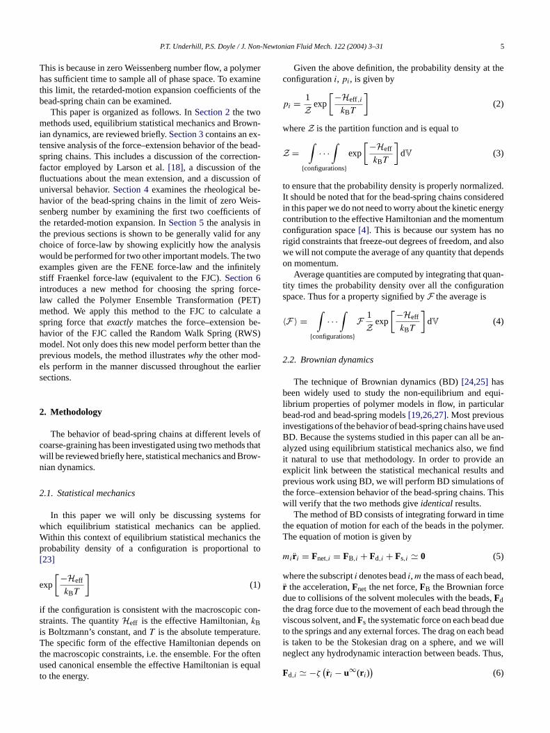
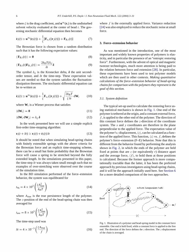


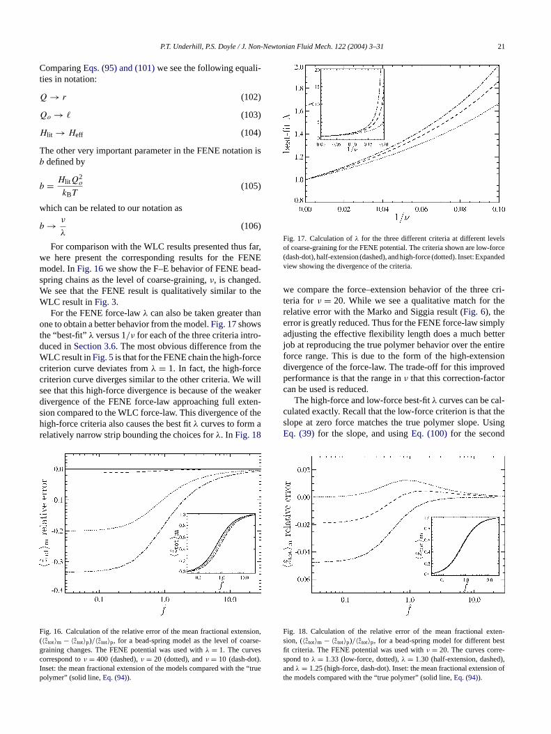


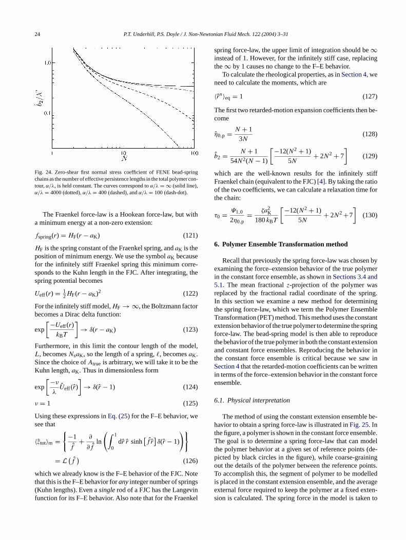

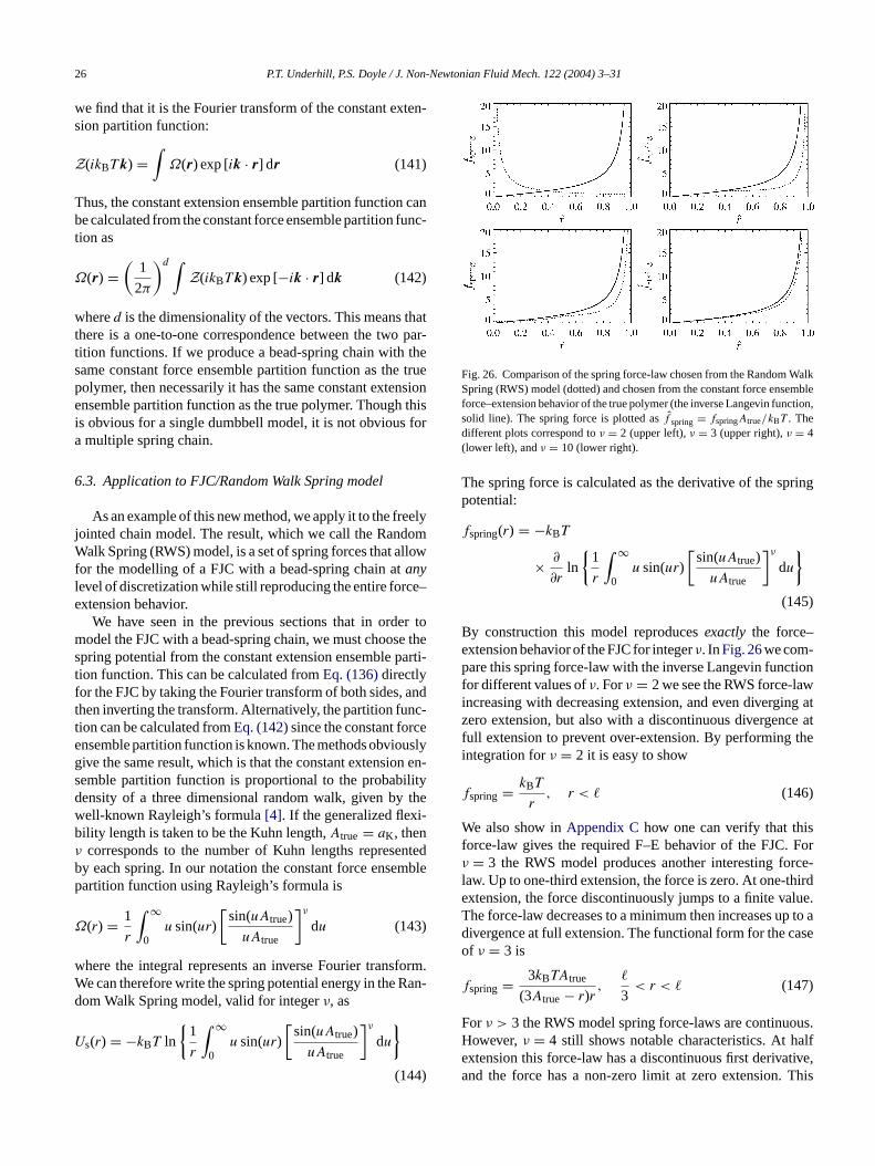


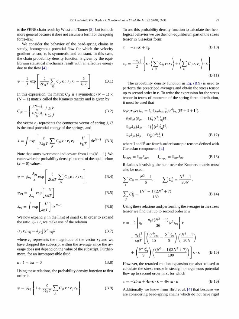


![STOCK: Structure Mapper and Online Coarse‐Graining Kit for ...praprot/publications/Bevc... · Ref. [16], so forth. Coarse-grained models also play an impor- ... aim of the presented](https://static.documents.pub/doc/80x56/602e2d476f46876e254196a2/stock-structure-mapper-and-online-coarseagraining-kit-for-praprotpublicationsbevc.jpg)


