HAL Id: hal-01756820 https://hal.archives-ouvertes.fr/hal-01756820 Submitted on 4 Jun 2018 HAL is a multi-disciplinary open access archive for the deposit and dissemination of sci- entific research documents, whether they are pub- lished or not. The documents may come from teaching and research institutions in France or abroad, or from public or private research centers. L’archive ouverte pluridisciplinaire HAL, est destinée au dépôt et à la diffusion de documents scientifiques de niveau recherche, publiés ou non, émanant des établissements d’enseignement et de recherche français ou étrangers, des laboratoires publics ou privés. On the Coexistence of Broadcast and Unicast Networks for the Transmission of Video Services Using Stochastic Geometry Ahmad Shokair, Youssef Nasser, Oussama Bazzi, Jean-François Hélard, Matthieu Crussière To cite this version: Ahmad Shokair, Youssef Nasser, Oussama Bazzi, Jean-François Hélard, Matthieu Crussière. On the Coexistence of Broadcast and Unicast Networks for the Transmission of Video Services Using Stochastic Geometry. IEEE Transactions on Broadcasting, Institute of Electrical and Electronics Engineers, In press, 64. hal-01756820
Transcript
HAL Id: hal-01756820https://hal.archives-ouvertes.fr/hal-01756820
Submitted on 4 Jun 2018
HAL is a multi-disciplinary open accessarchive for the deposit and dissemination of sci-entific research documents, whether they are pub-lished or not. The documents may come fromteaching and research institutions in France orabroad, or from public or private research centers.
L’archive ouverte pluridisciplinaire HAL, estdestinée au dépôt et à la diffusion de documentsscientifiques de niveau recherche, publiés ou non,émanant des établissements d’enseignement et derecherche français ou étrangers, des laboratoirespublics ou privés.
On the Coexistence of Broadcast and Unicast Networksfor the Transmission of Video Services Using Stochastic
To cite this version:Ahmad Shokair, Youssef Nasser, Oussama Bazzi, Jean-François Hélard, Matthieu Crussière. Onthe Coexistence of Broadcast and Unicast Networks for the Transmission of Video Services UsingStochastic Geometry. IEEE Transactions on Broadcasting, Institute of Electrical and ElectronicsEngineers, In press, 64. �hal-01756820�
SUBMITTED TO IEEE TRANSACTIONS ON BROADCASTING,JANUARY 29TH 2018 1
On the Coexistence of Broadcast and UnicastNetworks for the Transmission of Video Services
Using Stochastic GeometryAhmad Shokair, Youssef Nasser, Oussama Bazzi, Jean-Francois Helard, and Matthieu Crussiere,
Abstract—Following the increasing growth in the demand onmobile TV, hybrid broadcast/broadband networks emerged asa suitable approach to overtake the challenges introduced byeach network separately in order to enhance users’ experience.This paper presents two possible scenarios for a hybrid, spatiallyseparated, broadcast/broadband network to offer mobile TVlinear services for the end users. Namely, the first scenario isbased on shared spectrum access for both networks while thesecond one proposes a dedicated spectrum. Using a stochasticgeometry approach, the paper derives analytical formulationsfor both the probability of coverage and ergodic capacity. Theseformulations are then used to optimize the hybrid network interms of its key design parameters including the Broadcast (BC)coverage radii, the Broadband (BB) Base Stations’ (BS) density,and user satisfaction given in terms of spectral capacity. Theresults have shown that an optimal BC radius maximizing theprobability of coverage and capacity exists and it depends onthe BS density of the BB network. Other design parametershave been provided and analyzed leading to an optimal networkdeployment. To the best of the author’s knowledge, this paperpresents a first reference work dealing with the optimizationof the hybrid network with the coexistence of broadband andbroadcast networks, from stochastic geometry perspective, takinginto account the inter-cell interference.
RECENT years witnessed a high demand for linear ser-vices, especially mobile TV after the introduction of
smartphones and tablets. This was made possible by therapid advancement of both mobile-compatible Broadcast (BC)networks and mobile Broadband (BB) networks. However, themassive use of these smart devices has led to the extrava-gant use of BB resources leading to the so-called spectrumcrisis. Recently, among the different solutions proposed inthe literature, the co-existence between BC and BB networkshas emerged as a possible solution dealing with band hungryapplications, such as TV services. Therein, we firstly presentthe state-of-the-art technologies on linear services as well asthe different existing approaches for coexistence.
A. Mobile TV
The market for mobile TV is primarily directed by theglobal increase in the adoption of live stream services. MobileTV provides easy accessibility and availability of the desiredvideo content provided by several platforms. Those factorsencouraged consumers to prefer mobile TV over conventional
TV. Other factors like the ability for a user to watch his favoritecontent for affordable prices also played a major role in thespread of this service. The penetration of advanced hand-helddevices like smartphones and tablets made it even easier formobile TV to spread, particularly in growing markets likeIndia and China. Moreover, mobile TV has provided majorrevenues for mobile communication operators, TV providers,devices’ manufacturers. Mainly, time and space flexibility,accessibility, cost efficiency and spread of platform are themain factors for the spread of mobile TV in the last few years.This will also continue in the next few years as reported indifferent references [1], [2].
In practice, Mobile TV could be delivered to the end-usersin numerous methods. However, the latter could be groupedinto two categories: wireless BC or BB mobile networks.Digital Video Broadcast (DVB) project developed severalstandards that could be compatible with the handheld devicesincluding DVB-NGH in 2013, the successor to DVB-H intargeting handheld devices, and DVB-T2 in 2008, the secondgeneration terrestrial video broadcast protocol which wasdesigned to support both stationary and mobile devices [3].In the US, Advanced Television System Committee (ATSC)adopted ATSC-M/H for hand-held mobile devices in 2009.ATSC 3.0 is the new version of ATSC standards, which is sup-posed to support mobile TV for Ultra High Definition (UHD)videos [4]. Other mobile TV compatible standards were alsodeveloped in different regions of the world, like ISDB-TMMa mobile-targeted version of the Integrated Services DigitalBroadcasting (ISDB) in Japan in 2012 [5], Digital TerrestrialMultimedia Broadcast (DTMB) in China in 2006, and T-DMBby Digital Multimedia Broadcasting (DMB) in South Korea in2007 [6].
From the BB perspective, mobile TV could be provided bydifferent means. One way is to provide data by the regularmobile Unicast (UC) transmission. This method was madepossible by the recent advances in wireless mobile networksin terms of rate spectral efficiency namely the 3rd GenerationPartnership Project (3GPP) Long Term Evolution (LTE) [7].Multicast is also possible in LTE since a special point-to-multipoint interface called, Multimedia BC Multicast Services(MBMS), has been firstly introduced by 3GPP network in 2002and adopted by Universal Mobile Telecommunications System(UMTS) in 2011 [8], [9]. Evolved Multimedia Broadcast Mul-ticast Services (eMBMS), an advanced version of MBMS hasthen been adopted by LTE. Contrarily to UC, eMBMS deliverscontent to multiple users through shared radio resources [10],
SUBMITTED TO IEEE TRANSACTIONS ON BROADCASTING,JANUARY 29TH 2018 2
[11].In practice, both networks i.e., BC and BB present their
own limitations and advantages in terms of power, resources,performance, mobility, etc. Recently, hybrid networks basedon the coexistence of BC and BB networks have emerged asa candidate solution to reach the required quality of servicefor the end-users, but this requires a thorough analysis andoptimization of the transmission parameters.
B. Hybrid networks and related workBC networks have a good cost and spectral efficiency for a
large number of users, while this efficiency decays for loweruser density [12]. Contrarily, BB UC networks maintain a goodefficiency for a small number of users and suffer from overloaddue to limited spectral resources for a large number of users[13]. In addition, a BB base station has a limited coveragearea due to path loss and power constraints, while the BBnetwork provides wider coverage by means of multi-cells eachwith limited power. These facts encouraged the propositionof hybrid solutions, where BC and BB coexist to deliverlinear services. A hybrid network could then be consideredas an extension of the coverage area of the BC network bythe help of the BB network. It could also be considered asthe offloading of data traffic from the BB network to BCtransmission.
In literature, several studies have been conducted on hybridBB/BC networks, where the opportunities and challenges forthe hybrid approach for current and future implementationswere discussed in [12], [14], [15]. In general, one can classifythe coexistence approaches into two main types: (1) hybridcollaboration within same-area networks and (2) spatiallyseparated networks.
In same-area networks, authors in [16] proposed a systemmodel, criteria, and constraints for load switching in hybridcellular/BC network called switching bound concept. Heuckin [17] derived an analytical description of a hybrid networkand an IP data-cast architecture and discussed its performance.Wang et. al. in [18] designed a push-based content deliveryin a converged hybrid network to relieve the rapid growthin data traffic based on duration, popularity and size of themultimedia content. In [19], the authors proposed a convergedBB/BC platform for delivering 3D media to fixed and mobileusers guaranteeing a minimum QoS, alongside with an idealbusiness model for operators. Cornillet et al. studied theUC/BC cooperation from an energy point of view [20].Studieson the BC and BB coexistence from a spectral point of view,regarding overlapping and guard bands, were presented in[21] and [22]. Moreover, a unified BC layer targeting mobiledevices, based on DVB-T2 and LTE/eMBMS standards, wasproposed in [23]. Closely, the authors suggested in [24] anoverlay over the UC network by the BC tower enablingcooperative spectrum usage.
On the other hand, in spatially separated networks, theauthors of [25] proposed to maximize the global capacity fora hybrid BC/UC system in terms of power ratio between theBC tower and UC Base Station (BS), then derived a closed-form expression for ergodic capacity in the case of non-cooperative interfering coexistence. Authors in [26] planned
a stand-alone DVB-NGH and LTE and studied the benefitsfrom the cooperation between the two, then compared thosescenarios from energy consumption perspective in [27]. In[13], a study on the service coverage of an extension scenarioof a hybrid UC/BC network was proposed showing the exis-tence of an optimal operation mode where global throughputis maximized. Fam et al then introduced an analytical modelfor the optimal coverage to maximize hybrid network systemcapacity in [28], provided a theoretical analysis of the hybridnetwork performance in [29] and studied the energy efficiencyfor such model in [30].
C. Stochastic geometry modeling
In the previous works, the BB part of the hybrid networkwas usually modeled with the traditional grid model. However,such model is not accurate in terms of BS density anddistribution, especially in urban and suburban areas. Instead,recent studies have shown that stochastic geometry providesbetter, more realistic way of describing the distribution of amobile network [31], [32]. In this approach, the position ofBSs is set randomly using a point process. In fact, PoissonPoint Process (PPP) provides a decent tool to model the BSsdistribution with a single needed parameter, representing theaverage density of BSs in the service area [33]. PPP results inhaving, on average, the same number of points in a certainarea A, wherever A is chosen along the service area, thisnumber is equal to the product of the average density andthe area A. In [34], the authors investigated the accuracy ofthis model by testing against real implemented BSs in theUK, concluding that the stochastic geometry based modelis capable of modeling the network performance accurately.Andrews et al derived in [35] a general formula for the averageprobability of coverage and achievable throughput for a multi-cell BB network modeled by a PPP. The authors showed thata PPP is a pessimistic model compared to the conventionalgrid model, but is much more accurate in describing a realimplementation, where the estimated coverage by a PPP isslightly below the actual coverage compared to the grid modelwhich gives a higher estimate.
D. Contributions
This paper discusses the case of spatially separated hybridBC/BB networks. However, since eMBMS is not yet widelydeployed, this work considers a UC transmission for theBB network. Indeed, it was shown that UC could achievesignificantly high coverage rates with a proper allocation ofavailable resources [36]. In contrary to the previous works in[13], [28], [29], [30] where a grid model was used to describethe BB network, a more accurate PPP is used here to modelBSs positions. Moreover, our work considers the Inter-CellInterference (ICI) which has not been taken into account inthe literature. The main contributions of this paper could besummarized as follows:
1) Proposition of a model for two deployment scenarios thatcould be used for a spatially separated hybrid network,i.e. users inside BC area are served by the BC tower, andthe rest are served by nearest BB BS. The first scenario,
SUBMITTED TO IEEE TRANSACTIONS ON BROADCASTING,JANUARY 29TH 2018 3
named shared spectrum scenario, considers that BB BSsoutside BC area operate at the same frequency band asthe BC. The second, named dedicated spectrum scenario,assumes that those BSs operate at other frequenciessuch as TV White Space (TVWS). Those scenarios arecompared in terms of spectral efficiency.
2) Utilization of stochastic geometry tools by modeling theBS and users’ positions of the BB network as PPP model.
3) Consideration of ICI as one of the most influentialfactors in the design and obtained results. The effect ofinterference cancellation is also studied.
4) Derivation of the analytical expressions that evaluate theaverage probability of coverage for BC users, BB UCusers, and any user in the service area, for both scenarios.Similar derivations are provided for the user capacity ateach position in the hybrid model.
5) Optimization of the hybrid network in terms of designparameters, especially the BC radius and the density ofUC BSs.
The rest of this paper will be organized as follows. SectionII describes both model architectures, in addition to thederivation of some important probability distribution functions(pdfs) that will be used in the following sections. Sections III& IV include the derivation for average coverage probabilityand average user capacity respectively, for both scenarios, andintroduce some appropriate approximations when applicable.In section V, numerical simulations are conducted and com-pared to the analytical results. Then, a set of parameters isoptimized to maximize the coverage and rate, besides studyingthe effect of interference cancellation on the performance.Finally, section VI draws the conclusion of the paper andsuggests some future research directions.
II. PROPOSED SYSTEM MODEL AND SCENARIOS
In this section, we describe the hybrid network model in-cluding both transmission scenarios. In this work, we considerlinear TV serviced to M users, distributed in a wide circularservice area, resembling a typical metropolitan area, as shownin Fig. 1. The broadcast area is assumed to be occupying thecenter of the considered area. As for the broadband network,two main scenarios are considered. In the first scenario, UCBSs outside the broadcast area operate at the same frequencyas the BC area, while in the second scenario, UC BSs operateat another band such as digital TV white space, so there isno interference between UC and BC networks. Each scenariopresents its advantages and drawbacks in terms of spectrumallocation, interference level and hence system performance.Both approaches are in line with the current state-of-the-artconsiderations as detailed in the previous section.
The hybrid network consists of two Orthogonal FrequencyDivision Multiplexing (OFDM) systems:
1) A broadcasting system composed of a single High PowerHigh Tower (HPHT) site located at the center of theservice area.
2) A mobile broadband UC system composed of NBS basestation sites.
It is assumed that all the BB BSs transmit with the samepower PL, and the HPHT transmits with a power PD such that
PD > PL
The BS are located according to a PPP Φ with a densityλBS per squared Km. The users are distributed according toanother, independent, PPP Ψ with a density equal to λu. It isalso assumed that a user has the ability to connect to eithersystem depending on its position, i.e. if the user is within thecoverage area of the HPHT (rv < rb), then the user will beconnected to it. Else, it will be outside the BC region henceconnected to the nearest UC BS. This will result in a diskwith broadcast users inside, and a Voronoi tessellation for UCusers. An example of this network is shown in Fig. 1. For bothtransmission systems, the standard power loss propagationmodel is used, and it is assumed that all transmitter/receivercouples use Single Input Single Output (SISO) antennas.
-20 -15 -10 -5 0 5 10 15 20-20
-15
-10
-5
0
5
10
15
20
rb
rmax
BSout
Cell edges
UC user
HPHT
BSin
BC user
Service area
BC area
Fig. 1: An example of a service area, with 20 km radius, and10 km broadcast radius
A. Scenario 1: shared spectrum scenario
In the first scenario, the BC network operates at frequencyfD, while UC operates at fL for BSs within the BC area, andat fD for BSs outside the BC domain. This is briefed in Fig.2a. This arrangement will result in the following points:(a) Inter-cell Interference for UC users concerns the outside
area since the hybrid network is now operating at twodifferent frequencies for inside and outside BS. Theaverage level of interference for UC users depends onthe ratio of broadcast area to the service area,
(b) Inside users fed by the HPHT suffer from interferencefrom outside BS. However, this interference is variabledepending on the distance from HPHT and can be sig-nificantly small for non-edge users.
(c) Outside users fed by the UC BSs suffer from interferencefrom the HPHT. However, this interference is also vari-able depending on the distance from HPHT and can besignificantly small especially if the broadcast area is largeenough, and the power of HPHT is properly designed.
SUBMITTED TO IEEE TRANSACTIONS ON BROADCASTING,JANUARY 29TH 2018 4
(d) The interest of this scheme is clearly seen in terms ofbandwidth allocation as inside and outside users (of thebroadcast area) with TV services are operating at thesame frequency. This will be at the detriment of additionalinterference level as explained above.
The SINR for inside users is given by:
Si =PDgr−β
Vσ2 + ID
(1)
where PD is the transmission power by the HPHT, g representsthe random channel effect between the HPHT and the user,including shadowing and fading. rv is the distance betweenthe HPHT and the user, β represents the path loss exponentfor broadcast, σ2 is the noise power, and ID denotes the inter-ference on an inside user from outside BS. The interferenceis the sum of the powers of the received interfering signals.For a user in the broadcast area operating at frequency fD, allBSs in the UC area are considered as interferers, then ID isgiven by:
ID = ∑j∈Φ
PL h r−α
s, j (2)
where PL is the transmission power of UC BS, h representsthe channel random effect between the BS and the user, rs, jis the distance between a user and interfering BS j and Φ isthe set of all outside BS.
The SINR for outside users is given by:
So =PLhr−α
lσ2 + I1 + I2
(3)
where rl is the distance between the serving BS and the user,α represents the path loss exponent for UC, σ2 is the noisepower, and I1 and I2 denote the interference on an outside userfrom outside BS and the HPHT respectively. The interferenceon a user from interfering BS is given by:
I1 = ∑j∈Φ/b
PL h r−α
q, j (4)
and from the HPHT transmitter is given by:
I2 = BRPD g r−β
d (5)
where Φ/b denotes the set of all BSs in the UC area excludingthe serving BS for user under consideration. rq, j is the distancefrom an outside user and interfering BS j, and rd is thedistance from an inside user to the HPHT transmitter. Br isthe ratio between the BW of the BC and that of UC. Sincein general, the bandwidth (BW) of the BB network is higherthan that of the BC where both are overlapping, the ratio canbe written as following:
BR = min(1,BWBC
BWUC) (6)
where BWBC and BWUC are the BW of BC and UC respectively.
B. Scenario 2: dedicated spectrum scenario
The second scenario considered in this paper differs fromScenario 1 in the spectrum allocation. Indeed, here the BCHPHT operates at fD, UC BS inside BC area operate at fL,while the BS outside BC domain operate at fW , a sub-bandof the TV white space, where fL, fW and fD don’t overlap.This scenario is summarized in Fig.2b. This will result in thefollowing points:(a) Compared to shared spectrum scenario, ICI for UC is
significantly reduced due to the usage of three differentfrequencies.
(b) Contrarily to Scenario 1, inside users, fed by the HPHTwill only be limited by path loss and noise, and will notsuffer from any interference.
(c) Outside users fed by the UC BS suffer only from ICIproduced by outside cells.
(d) The interference is limited at the expense of additionalbandwidth allocation.
The SNR for inside users is given by:
Si =PDgr−β
Vσ2 (7)
The SINR for outside users is given by:
So =PLhr−α
lσ2 + I1
(8)
The difference from shared spectrum scenario is that ID, theinterference from outside BS on inside users, and I2, theinterference from HPHT on outside users, are both eliminatedfrom the equations.
C. PDFs of main separation distances
Three distances shown in figure 3 are particularly importantin the derivations that will follow: (1) the distance rd betweenthe UC user and the HPHT transmitter, (2) the distance rvbetween a BC user and the center, and (3) the distance rlbetween a UC user and its serving BS. Since both BS and userspositions are random, those distances are random as well, andtheir distributions are needed in the derivation of coverage andcapacity.
The CDF of rd is given by:
Frd (Rd) = P[rd < Rd ]
=A(Rd ,rb)
AUC
=πR2
d−πr2b
πr2max−πr2
b
=1
r2max− r2
bR2
d−r2
b
r2max− r2
b
(9)
where A(Rd ,rb) is the area limited by the two circles of radiusRd and rb. The PDF of rd will then be:
frd (Rd) =dFrd (Rd)
dRd
=2
r2max− r2
bRd
(10)
SUBMITTED TO IEEE TRANSACTIONS ON BROADCASTING,JANUARY 29TH 2018 5
rl represents the distance to the serving BS. That meansthat the area between the user and the serving BS is emptyfrom any interfering BS. For a PPP in R2, the null probabilityin an area A is exp(−λA) [35]. Then, the CCDF of rl is asfollowing:
Frl (Rl) = P[rl < Rl ]
= 1− exp(−λA)
= 1− exp(−λ
min(rmax,rd+Rl)∫max(rb,rd−Rl)
2θv dv)
= 1− exp(−2λ
min(rmax,rd+Rl)∫max(rb,rd−Rl)
arccos(v2 + r2
d −R2l
2v rd)vdv)
(12)
Then, the PDF of rl is given by:
frl (Rl) =d
drl
[exp(−2λ
min(rmax,rd+Rl)∫max(rb,rd−Rl)
arccos(v2 + r2
d −R2l
2v rd)vdv)
)](13)
where the area A could be found as shown in Fig. 4.Approximation of the PDF of rl: Eq. (13) is very hard to
express and interpret, and therefore will be hard to be used inthe sequel. Alternately, it could be easily verified that if theedge cases are ignored, and the BS density exceeds a certainlow-value threshold, the area to be processed is simpler, andcould be seen as a complete disk with radius rl . Thus the PDFof rl could be reduced to:
f ∗rl(Rl) = 2πλ rl exp(−πλ r2
l ) (14)
It can clearly be seen that even though the approximation ismuch simpler than the exact value, it completely ignores therelative position to the center and the broadcast radius rb. Inthe sequel, this approximation will be used when necessary,like in the estimation of of average coverage probability forBC users in (17) and (32) and UC users in (23) and (34),where both the exact formula and the approximation could beused.
III. AVERAGE PROBABILITY OF COVERAGE
In this section, we derive the analytical expressions for theaverage probability of coverage of inside users (i.e. broadcastregion), outside users (i.e. UC region), and the average proba-bility of coverage of any user at any position. The probabilityof coverage is defined as the probability of a user to havea SINR value higher than a certain threshold T [35]. Inorder to clarify the derivation steps, Table I summarizes theused symbols. Since shared spectrum scenario and dedicatedspectrum scenario have slight differences in the derivationof final expressions, the derivation for the first scenario isexplained, while in the second scenario, only the final resultis stated with indication on the differences.
SUBMITTED TO IEEE TRANSACTIONS ON BROADCASTING,JANUARY 29TH 2018 6
Fig. 4: Calculation of area limited by the circle of radius Rl ,service area circle, and broadcast area circle
TABLE I: Table of used symbols
Symbol indication
rmax Radius of service arearb Radius of BC arearl Distance from user under UC to serving BSrd Distance from user under UC HPHTrq Distance from user under UC to interfering BSrv Distance from user under BC to HPHTrs Distance from user under BC to interfering BSPD Tx power of HPHTPL Tx power of BSg Term including random HPHT-user channel conditionsh Term including random BS-user channel conditionsα Path loss exponent for BS and a userβ Path loss exponent for HPHT and a userσ2 Noise power at the receiverλBS Density of BS PPPλu Density of users PPPT SINR thresholdPc Probability of coverage for a general user
Pc/i Probability of coverage for a BC userPc/o Probability of coverage for a UC userC Capacity per Hz for a general userCi Capacity per Hz for a BC userCo Capacity per Hz for a UC user
A. Shared Spectrum Scenario
1) Coverage for BC users: For inside users under broad-cast, the average probability of coverage is given by:
Pc/i = Erv
[P(Si > T/rv)
]= Erv
[P(
PDgr−β
Vσ2 + ID
> T/rv)]
(a)=
rb∫0
P(g >Trβ
VPD
(σ2 + ID)/rv) frv(rv)drv
=2r2
b
rb∫0
P(g >Trβ
VPD
(σ2 + ID)/rv)rvdrv
(15)
where (a) follows the independence of the distribution of rvand the channel g. Here, we can derive:
P(g >Trβ
VPD
(σ2 + ID)/rv) = EID[P(g >
Trβ
VPD
(σ2 + ID)/ID,rv)]
(b)= EID
[exp(−τTrβ
VPD
(σ2 + ID))]
= exp(−τTrβ
V σ2
PD
)EID[exp(−τTrβ
VPD
ID)]
= exp(−τTrβ
V σ2
PD
)LID
(−τTrβ
VPD
)(16)
where (b) follows the assumption of an exponential distribu-tion of g: g ∼ exp(τ). LID(s) is the Laplace transform of IDevaluated at s. Then:
Pc/i =2r2
b
rb∫0
exp(−τTrβ
V σ2
PD
)LID
(−τTrβ
VPD
)rvdrv (17)
The exact derivation for the Laplace transform LID(s) resultsin the following formula:
LID(τTrβ
v
PD) =exp
(−2λ
( rmax−rv∫0
πrs
1+ µPDrαs
T τPLrβ
b
drs
+
rmax+rv∫rmax−rv
arccos( r2v+r2
s−r2max
2rvrs)
1+ µPDrαs
T τPLrβ
b
rsdrs
−rb−rv∫0
πrs
1+ µPDrαs
T τPLrβ
b
drs
−rb+rv∫
rb−rv
arccos( r2v+r2
s−r2b
2rvrs)
1+ µPDrαs
T τPLrβ
b
rsdrs
))
(18)
It is very clear that Eq.(18) could be reduced to simpleclosed-form expressions, hence two different approximationsare provided as follows.
Approximation 1 of Eq.(18): Here, it is assumed that dueto high BC transmission power, interference is not effectivebeyond certain point, so the effective interference could bereduced to the disk surrounding a user, with a radius equal tothe distance of HPHT from that user. In this case, (18) can bewritten as:
L ∗ID(
τTrβv
PD) = exp
(−2λ
min(rmax−rv,rv)∫rb−rv
π− arccos( r2v+r2
s−r2max
2rvrs)
1+ µPDrαs
T τPLrβ
b
rsdrs
)(19)
Approximation 2 of Eq.(18): A second approximationcould be obtained by assuming that interference is produced bya single interferer placed on the closest point to a user directlyon the BC/UC border. This approximation is not generallyaccurate, but it significantly reduces the complexity of thecalculations. The Laplace transform yields:
L ∗∗ID (
τTrβv
PD) =
1
1+ τPLTrβ
VµPD(rb−rv)α
(20)
SUBMITTED TO IEEE TRANSACTIONS ON BROADCASTING,JANUARY 29TH 2018 7
The derivations of the Laplace transform, and the approxima-tions could be found in Appendix B.
Eq.(17) indicates, as expected, that increasing the radiusof BC area without a suitable increase in broadcast powerwill decrease the average coverage probability for BC usersespecially for edge users with a high value of rv causing bothterms inside the integral to be significantly smaller. In fact,the second approximation shown in (19) indicates that the BCradius rb has a significant additional effect since it appearsin the denominator with an exponent which is higher than 2.The equations also indicate that increasing the BS transmissionpower PL will reduce the coverage for BC users, with the BS’sdensity λ has a similar effect.
2) Coverage for UC users: Outside users are connectedto the nearest BS, operating at fD, and served using unicast.Those users suffer from two sources of interference due to theHPHT power and the other outside BSs. The probability ofcoverage of the outside users could be written as:
Pc/o = Erd ,rl
[P[So > T/rd ,rl ]
]= Erd ,rl
[P[ PLhr−α
lσ2 + I1 + I2
> T/rd ,rl]]
=
rmax∫rb
frd (rd)
2rmax∫0
frl (rl)P[h >Trα
lP
(σ2 + I1 + I2)/rd ,rl ]drldrd
(21)where the last step follows the independence of the distributionof rd , rl and the channel random effect represented by h. Thedistance rd between an outside user and the HPHT variesbetween rb in the case of a user on the edge of the broadcastarea, and rmax in the case of a user on the edge of the servicearea. On the other hand, rl , the distance between an outsideuser and its serving base station, varies between zero and2rmax. However, practically the upper limit is likely much less,especially when the BS density is high enough. Again, theprobability of coverage for outside users can be deduced fromthe previous equation by:
P[h >Trα
lP
(σ2 + I1 + I2)/rd ,rl ]
= EI1
[EI2
[exp(−µTrα
lPL
(σ2 + I1+ I2))]]
= exp(−µTrα
l σ2
PL
)LI1/rd
(µTrα
lPL
)LI2/rd
(µTrα
lPL
) (22)
where the first step follows the independence of the inter-ference from HPHT and the interference from surroundingBSs, and follows also the exponential distribution of thechannel parameter h: h ∼ exp(µ). Plugging this into (21), andsubstituting frd (rd) by its formula derived in (10), we get:
Pc/o =2
r2max− r2
b
rmax∫rb
rd
rmax∫0
frl (rl)exp(−µTrα
l σ2
PL
)LI1/rd ,rl
(µTrα
lPL
)LI2/rd ,rl
(µTrα
lPL
)drldrd
(23)
LI1/rd
(µTrα
lPL
)and LI2/rd
(µTrα
lPL
)are the Laplace transform
of I1 and I2 respectively. LI1/rd
(s)
can be evaluated at cer-
tain values of rl and rd . The exact derivations, reported inAppendix C, lead to the following formula:
LI1/rd
(µTrα
lPL
)= exp
(−2λ
( rmax−rd∫min(rl ,rmax−rd)
πrq
1+ 1T
(rqrl
)α drq
+
rmax+rd∫max(rl ,rmax−rd)
arccos(r2d+r2
q−r2max
2rdrq)
1+ 1T
(rqrl
)α rqdrq
−rd+rb∫
max(rl ,rd−rb)
arccos(r2d+r2
q−r2b
2rdrq)
1+ 1T
(rqrl
)α rqdrq
))(24)
Approximation of the LT in (24): In order to reducethe complexity of (24), an approximation could be made, byassuming that the major source of interference is due to thefirst term which represents the disk limited by the BC diskand the service area circle. From the above formula, this willlead the following:
L ∗I1/rd
(µTrα
lPL
)= exp
(−2λ
rmax−rd∫min(rl ,rmax−rd)
πrq
1+ 1T
(rqrl
)α drq
)(25)
On the other hand, LI2/rd
(s)
could be evaluated for certainvalues of rd as follows:
LI2/rd
(s)= Eg
[exp(−sI2)
]= Eg
[exp(−sBRPDgr−β
d )]
=1
1+ sBRPDr−β
dτ
(26)
then
LI2/rd
(µTrα
lPL
)=
1
1+ BRT µPDr−β
d rαl
τPL
(27)
From the three terms in (24) or from the approximationmade in (25) one can conclude that the UC transmissionpower doesn’t affect the Laplace transform of the inter-cell interference. However, increasing PL boosts the overallcoverage by increasing the other two terms in (23). Moreover,taking into account the approximations done in (14) and (25),the effect of the BS density λ is not similarly clear. Fromone point, increasing λBS increases the linear part in (14),but decreases the exponential parts in (14) and (25). Thus theoverall effect of λBS depends on other factors that appear inthe exponential and control the decay rate like T and α . Notethat for the case of Br equal to 0, indicating no overlapping,the equation returns to the case where no interference fromthe BC on the UC exists, and LI2/rd
(µTrα
lPL
)is meaningless,
and the coverage probability will be similar to that scenario2, which will be later shown in (34).
SUBMITTED TO IEEE TRANSACTIONS ON BROADCASTING,JANUARY 29TH 2018 8
3) Coverage for any user in the service area: Since theusers are randomly and uniformly distributed over the servicearea, then the probability of a user to be in the broadcast regionis
Pi =ABC
Atotal
=r2
br2
max
(28)
where ABC is the BC area, and Atotal is the service area.Consequently, the probability of a user to be in the UC regiondomain is
Po = 1−r2
br2
max(29)
and the total probability of coverage for a general user in theservice area will be
Pc = PiPc/i +PoPc/o (30)
B. Dedicated Spectrum ScenarioThe derivation steps of Scenario 2 are similar to that of
Scenario 1 with one major difference: the elimination of ID andI2 and their related equations. Thus the probability of coveragefor inside users will be as follows:
Pc/i =2r2
b
rb∫0
exp(−µTrβ
V σ2
PD
)rvdrv (31)
using equation 3.381/8 in [37] this equation could be writtenin the form:
Pc/i =2r2
b
γ
(2β,
µT σ2rβ
bPD
)β ( µT σ2
PD)2/β
(32)
where γ(a,x) is the incomplete gamma function given by:
γ(a,x) =∞∫
0
e−vva−1dv (33)
In addition, the probability of coverage of outside users couldbe written as :
Pc/o =2
r2max− r2
b
rmax∫rb
rd
rmax∫0
frl (rl)exp(−µTrα
l σ2
PL
)LI1/rd
(µTrα
lPL
)drldrd
(34)
In Scenario 2, one can notice that coverage of inside users isrelated only to the parameters of the BC, and it is independentof the unicast parameters. In addition, the coverage of outsideusers is dependent only on UC parameters and rb. This meansthat in general, the coverage of inside and outside users willincrease with this model, but at the expense of using anadditional frequency band.
IV. AVERAGE CAPACITY DERIVATION
In this section, we consider the average capacity for abandwidth unit. As in the previous section, derivations forscenario 1 are described, and the final results of the secondscenario follow.
A. Shared Spectrum Scenario
We consider the average capacity for a bandwidth unit tobe as follows:
C = log2[1+SINR] (35)
1) Capacity for inside users: the average capacity for theinside users served by broadcast can be evaluated as:
Ci = E[log2(1+Si)]
= EΦ,g[log2(1+PDgr−β
Vσ2 + ID
)]
=
rb∫0
frv(rv)E[
log2(1+PDgr−β
Vσ2 + ID
)/rv
]drv
(a)=
rb∫0
frv(rv)
∞∫0
P[
log2(1+PDgr−β
Vσ2 + ID
)> t/rv
]dtdrv
=
rb∫0
frv(rv)
∞∫0
P[g >
(2t −1)rβ
VPD
(σ2 + ID)/rv
]dtdrv
=
rb∫0
frv(rv)
∞∫0
EID
[exp(−τ(2t −1)rβ
v
PD(σ2 + ID/rv)
)]dtdrv
=2r2
b
rb∫0
rv
∞∫0
exp(−τ(2t −1)rβ
V σ2
PD
)LID
(τ(2t −1)rβ
VPD
)dtdrv
(36)where (a) follows from
E[X]=
∞∫0
P(
X > x)
dx (37)
LID
(s)
is calculated in Appendix B. It could be used by
substituting s by τ(2t−1)rβ
VPD
.2) Capacity for outside users: Using similar analysis, the
average capacity for outside users is given by:
Co = Erd ,rl ,h
[log2(1+So)
]=
rmax∫rb
frd (rd)
2rmax∫0
frl (rl)E[
log2
(1+
PLhr−α
lσ2 + I1 + I2
)/rd ,rl
]drldrd
(a)=
rmax∫rb
frd (rd)
2rmax∫0
frl (rl)∫
P[
log2
(1+
PLhr−α
lσ2 + I1 + I2
)> t/rd ,rl
]dtdrldrd
=
rmax∫rb
frd (rd)
2rmax∫0
frl (rl)
∞∫0
P[h >
(2t −1)hrαl
PL(σ2 + I1 + I2)/rd ,rl
]dtdrldrd
(b)=
rmax∫rb
frd (rd)
2rmax∫0
frl (rl)
∞∫0
EI1,I2
[exp(−µ(2t −1)rα
lPL
(σ2 + I1 + I2))/rd ,rl
]dtdrldrd
=2
r2max− r2
b
rmax∫rb
rd
2rmax∫0
frl (rl)
∞∫0
exp(−µ(2t −1)rα
l σ2
PL
)LI1/rd
(µ(2t −1)rαl
PL
)LI2/rd
(µ(2t −1)rαl
PL
)dtdrldrd
(38)
SUBMITTED TO IEEE TRANSACTIONS ON BROADCASTING,JANUARY 29TH 2018 9
where (a) also follows from (37), and (b) follows the exponen-tial distribution of h. The final step follows the independencebetween I1 and I2.
3) Total average capacity: Similar to the probability ofcoverage of a user at any position, the average capacity willbe
C = PiCi +PoCo (39)
B. Dedicated Spectrum Scenario
In scenario 2, the capacity for inside and outside users aresimilar to that of model 1, but again, with the elimination ofterms related to ID and I2. The capacity of inside users couldthen be derived and written as:
Ci =1
ln(2)2r2
b
rb∫0
rv
∞∫0
exp(−τ(et −1)rβ
V σ2
PD
)dtdrv (40)
By some rearrangement, and the use of equation 3.327 in [37],the capacity can be written as:
Ci =1
ln(2)2r2
b
rb∫0
rv exp(
τσ2rβv
PD
)[−Ei
(− τσ2rβ
v
PD
)]drv (41)
where Ei(x) is the exponential integral function given by:
Ei(x) =−∞∫−x
e−u
udu (42)
Moreover, the capacity for outside users is given by:
Co =2
r2max− r2
b
rmax∫rb
rd
2rmax∫0
frl (rl)
∞∫0
exp(−µ(2t −1)rα
l σ2
PL
)LI1/rd
(µ(2t −1)rα
lPL
)dtdrldrd
(43)
C. Effective Capacities
All previously calculated capacities are per frequency unit.However, to derive the average user capacity, multiplicationby the occupied bandwidth is needed. But for the BC users,the average effective capacity is related to the transmitted bitrate, which is the required capacity for a proper reception ofthe service or Creq. Hence, the total BC capacity is given by:
CBC = ∑m∈M
Creqam (44)
where M is the set of users within BC region, and am a binaryvariable that is equal to 1 if the SINR for user m named SINRmis greater or equal to the threshold T and 0 otherwise, thusindicating if user m is receiving the service properly or not.
The average BC capacity in the broadcast area could bethen calculated as follows:
[CBC] =CreqPc/iλU πr2b (45)
where λU πr2b is equal to the average number of users inside
BC area.
Similarly, for UC users, the total cell capacity is given by:
CUC,celln = ∑
m∈Cn
Cuserm bm,n (46)
where Cn is the set of users in the cell, Cuserm is the capacity
for user m, and bm is a binary variable that is equal to 1 ifuser m is connected to the service i.e. SINRm > T . Cuser
m couldbe found as follows:
Cuserm = NRB
m BRB log2(1+SINRm) (47)
where NRBm is the number of resource blocks allocated to user
m, and BRB is the bandwidth of a single resource block. Sofor the UC network, the total capacity will be:
CUC = ∑n∈N
CUC,celln (48)
Thus, the average UC capacity could be derived as:
[CUC] = [NRB]BRBCoPc/oλU π(r2max− r2
b) (49)
where λU π(r2max− r2
b) sums the average number of UC users,and [NRB] denotes the average number of resource blocksassigned for a user. Finally the total average capacity couldbe given as:
[Csys] = [CBC]+ [CUC] (50)
Those values are used to derive the capacity of the hybridsystem for both scenarios.
V. SIMULATION RESULTS
To compare the formulations derived previously with sim-ulations, numerical and Monte-Carlo (MC) simulations havebeen conducted. Numerical analysis was also used to findoptimal operating points for different of system parameters.The service area selected is of 30 km radius, with variableBC radius. Unless otherwise mentioned, the density of BSsis equal to 0.15BS/km2. Default simulation settings are sum-marized in Table II. The isotropic transmission power of BSsis set to 1200 W, and the isotropic transmission power of theHPHT is set to 33 kW.
TABLE II: Simulation setting
Parameter Value
rmax 30 kmrb 10 kmPD 33 kWPL 1.2 kW
BWBC 8 MHzBWUC 10 MHz
µ 1τ 1α 3.4β 3.2σ2 -100 dBmλBS 0.15BS/km2
λu 1user/km2
T 0 dB
SUBMITTED TO IEEE TRANSACTIONS ON BROADCASTING,JANUARY 29TH 2018 10
A. Simulation and analytical results in terms of coverageCCDF
Firstly, to compare the analytical expressions with MCsimulation results, the CCDF of the probability of coverageis calculated for inside users, outside users, and any user inthe service area as shown in Fig. 5a, 5b, and 5c respectivelyfor shared spectrum scenario, and in Fig. 6a, 6b, and 6crespectively for dedicated spectra scenario.
Both Fig. 5a and 6a show a very good convergence betweenthe simulation and the analytical results. Fig. 5b and 6b showa very high accuracy as well, with error ranging from 1to 2%. Fig.5c and 6c verify the derived formulations andthe different probability expressions in the previous sections.The first approximation for BC users presented in equation(19), and the approximation for UC users provided by Eq.(25) produce very close values to both simulation results andderived equations. The second approximation for the BC usersprovided by Eq. (19) is accurate for high threshold values, andlooses its accuracy for low threshold values, i.e. below 3dB.However, the use of these approximations reduces significantlythe processing time for the analytical derivations. Fortunately,these approximations work well with the practical transmissionparameters.
The problem turns out now to find the optimal set ofparameters which maximizes the probability of coverage andusers’ capacity.
B. Optimization of the Hybrid Network
Among the different design parameters, it is very clear thatthe first parameter to optimize is the radius (i.e. the coverage)of the broadcast area for both scenarios. Fig. 7a and 7b showthe probability of coverage vs the BC radius for a generaluser in the service area for UC BS densities of 0.05BS/km2
and 0.15BS/km2 for both scenarios. The results show thatfor a small value of rb, where most users are UC users, theprobability of coverage Pc will be limited by the achievablePc in the UC network. When the BC radius rb increases, moreusers are being covered by the BC network and thus the totalPc increases. However, when rb is increased too much, edgeusers associated with BC become out of coverage due to highinterference, pathloss and noise levels. Optimal values of rbvary between 8 and 12 km.
Both figures show that the required threshold T has a hugeeffect on the coverage probability, but a limited effect on theoptimal radius of BC area. In addition, results show that forshared spectrum scenario, increasing λBS pushes the optimalpoint towards smaller values. This effect is not as clear inscenario 2. The main reason could be that in Scenario 1,adding more UC BS add more interference to BC users, andconsequently, limits the BC sub-network efficiency. Moreover,a comparison between the two plots shows that there is nosignificant difference between the two cases in terms of theoptimal radius, and it is limited to a shift of around onekilometer in some cases.
Similar remarks could be concluded from Fig. 8a and 8b,showing the total system capacity as a function of rb for thetwo values of UC BS density mentioned above. Both figures
show that an optimal point can be determined for the set ofparameters under test.
Since the average values, in general, could be misleading,and in order to highlight the effect of the position on thecoverage, a test was done without the last averaging overposition with respect to the center in Eq. (17) and (23) forScenario 1, and Eq. (32) and (34) for Scenario 2. Fig. 9a and9b show a cross-section of the service area, from the centerto the edge, with the coverage probability at each point withdistance R from the center of the service area, for two differentvalues of λBS, and their corresponding optimal BC radius rbfor both scenarios. Results show that BC users have excellentcoverage for both cases near the HPHT as expected, but thisvalue drops dramatically for scenario 1 on the BC border dueto interference, and the drop is more skewed when the densityis higher. In the second scenario, the drop is smoother, andit is not affected by the density of BSs. Moreover, UC has astable coverage value over most of its region except at bothboundaries, with a higher average for higher density network,and with a slight outperformance for the dedicated spectrumscenario. One could mention the main changes in the BC/UCborder region. In shared spectrum scenario, users on both sidesof the UC/BC borders suffer from severe interference levels,which results in the gap seen in Fig.9a with a probability ofcoverage that drops down to 0.11 and 0.1 with λBS equal to0.15 and 0.05BS/km2 respectively. In contrary, this gap is notas significant in Fig. 9b that corresponds to dedicated spectrascenario, as it is limited by the slight change in operating BSsdensity near the border.
Fig. 10a and 10b show the achievable capacity by 90% ofthe users in the service area for both scenarios. Higher UCnetwork density achieves higher capacities, mainly due to theadvantage of such networks in providing higher number ofaccess points and then resources. Results also show that forshared spectrum scenario, a dense network requires smaller BCarea to achieve its optimal values, while in dedicated spectrascenario, the density doesn’t affect much the optimal point.
C. Effect of BS density
The second main design parameter for the hybrid networkis the density of the BS providing unicast. To study theeffect of the BS’s density, probability of coverage, averageuser capacity, and average system capacity for inside, outside,and general user are calculated for different values of λBS,for both scenarios under study, for values of rb around theoptimal values found in the previous section, and are shownin Fig.11 and 12. For shared spectrum scenario, in generala low-density network will produce less interference on BCusers, and thus those users will have better coverage andcapacity. Nevertheless, low-density network means that UCusers are on average far from their BS and thus have lesscoverage and capacity. The growth of coverage for UC userswith the increase of λBS is faster than the decay of the coveragefor BC users, thus the total coverage increases, until a pointwhere further increase doesn’t produce additional capacity orcoverage since the interfering BSs are becoming closer totypical UC user. In the setting used here, one can conclude
SUBMITTED TO IEEE TRANSACTIONS ON BROADCASTING,JANUARY 29TH 2018 11
Threshold SINR [dB]
-10 -5 0 5 10 15 20
Pci
0
0.1
0.2
0.3
0.4
0.5
0.6
0.7
0.8
0.9
1
rb=10km , λ = 0.05 BS/km2
Analytical exact
Approx. 1, eq(19)
Approx. 2, eq(20)
simulation
(a) Inside users Pc/i
Threshold SINR [dB]
-10 -5 0 5 10 15 20
Pco
0
0.1
0.2
0.3
0.4
0.5
0.6
0.7
0.8
rb=10km , λ = 0.05 BS/km2
Analytical exact
Approx. 1, eq(25)
Simulation
(b) Outside users Pc/o
Threshold SINR [dB]
-10 -5 0 5 10 15 20
Pc
0
0.1
0.2
0.3
0.4
0.5
0.6
0.7
0.8
rb=10km , λ = 0.05 BS/km2
Analytical exact
Approx. 1, eq(19,25)
Approx. 2, eq(20,25)
simulation
(c) General userPc
Fig. 5: CCDF of probability of coverage Pc for shared spectrum scenario
Threshold SINR [dB]
-10 -5 0 5 10 15 20
Pci
0
0.1
0.2
0.3
0.4
0.5
0.6
0.7
0.8
0.9
1
rb=10km , λ = 0.05 BS/km2
Analytical exact
Simulation
(a) Inside users Pc/i
Threshold SINR [dB]
-10 -5 0 5 10 15 20
Pco
0
0.1
0.2
0.3
0.4
0.5
0.6
0.7
0.8
rb=10km , λ = 0.05 BS/km2
Analytical exact
Approx. 1, eq(23)
Simulation
(b) Outside users Pc/o
Threshold SINR [dB]
-10 -5 0 5 10 15 20
Pc
0
0.1
0.2
0.3
0.4
0.5
0.6
0.7
0.8
rb=10km , λ = 0.05 BS/km2
Analytical exact
Approx. 1, eq(23)
Simulation
(c) General userPc
Fig. 6: CCDF of probability of coverage Pc for dedicated spectra scenario
Broadcast radius rb (km)
0 5 10 15 20 25 30
Pro
babili
ty o
f covera
ge P
c
0
0.1
0.2
0.3
0.4
0.5
0.6
0.7
0.8
PD
= 33kW , PL = 1.2kW , α = 3.4 , β = 3.2
λBS
= 0.05 , T=-7dB
λBS
= 0.15 , T=-7dB
λBS
= 0.05 , T=0dB
λBS
= 0.15 , T=0dB
λBS
= 0.05 , T=3dB
λBS
= 0.15 , T=3dB
(a) Shared spectrum scenario
Broadcast radius rb (km)
0 5 10 15 20 25 30
Pro
babili
ty o
f covera
ge P
c
0
0.1
0.2
0.3
0.4
0.5
0.6
0.7
0.8
PD
= 33kW , PL = 1.2kW , α = 3.4 , β = 3.2
λBS
= 0.05 , T=-7dB
λBS
= 0.15 , T=-7dB
λBS
= 0.05 , T=0dB
λBS
= 0.15 , T=0dB
λBS
= 0.05 , T=3dB
λBS
= 0.15 , T=3dB
(b) Dedicated spectra scenario
Fig. 7: Probability of coverage for both scenarios vs. the BC radius rb for -100 dBm noise power
that 0.15BS/km2 is enough for nearly maximum coverage and0.1BS/km2 for maximum user capacity.
Similarly, Fig. 11c and 12c shows the total average systemcapacity for the hybrid network as a function of UC BSdensity. The results have the same indication, a BS densityequal to 0.15BS/km2 is enough to have optimal system ca-pacity. In dedicated spectrum scenario, however, the densitydoesn’t affect the inside users’ capacity and coverage, andconsequently the coverage, average user capacity, and averagesystem capacity are higher in general. However, Scenario 2
doesn’t significantly shift the value on which the coverage andcapacity become stable. In practice, the control of BS densitycan be done by turning off the service transmission of selectedBSs but this leads to a new model of a PPP network which isout-of-scope in this paper.
D. Interference cancellation
In all the testings performed so far, the induced interferencewas fully taken into account as no interference cancellationwas supposed to be carried out. Here the effect of potential
SUBMITTED TO IEEE TRANSACTIONS ON BROADCASTING,JANUARY 29TH 2018 12
Fig. 8: Average system capacity vs. the BC radius rb for -100 dBm noise power, Creq of 2 Mbps, and 1400 users
Distance from center (km)
0 5 10 15 20 25
Pc
0
0.1
0.2
0.3
0.4
0.5
0.6
0.7
0.8
0.9
1
λBS
=0.05 BS/km2, r
b=12 km
λBS
=0.15 BS/km2, r
b=9 km
(a) Shared spectrum scenario
Distance from center (km)
0 5 10 15 20 25
Pc
0
0.1
0.2
0.3
0.4
0.5
0.6
0.7
0.8
0.9
1
λBS
=0.05 BS/km2, r
b=11 km
λBS
=0.15 BS/km2, r
b=10 km
(b) Dedicated spectra scenario
Fig. 9: Probability of coverage as a function of distance from center for two values of λBS and their corresponding values ofrb for −100dBm noise power and T=0 dB
Broadcast radius rb (km)
0 5 10 15 20 25 30
Achie
vable
capacity for
90%
of users
(bit/s
ec/H
z)
0
0.02
0.04
0.06
0.08
0.1
0.12
PD
= 33kW , PL = 1.2kW , α = 3.4 , β = 3.2
λBS
= 0.05
λBS
= 0.15
(a) Shared spectrum scenario
Broadcast radius rb (km)
0 5 10 15 20 25 30
Acheiv
able
capacity for
90%
of users
(bit/s
ec/H
z)
0
0.02
0.04
0.06
0.08
0.1
0.12
PD
= 33kW , PL = 1.2kW , α = 3.4 , β = 3.2
λBS
= 0.05
λBS
= 0.15
(b) Dedicated spectra scenario
Fig. 10: Achievable user capacity per unit frequency vs. the BC radius rb for -100 dBm noise power and T= 0 dB
interference cancellation technique, modeled with a cancella-tion factor γ is studied. In fact, the SINR formulas are slightly
modified versions of Eq. (2) and Eq. (3) to include the newfactor. For shared spectrum the modified formula for BC and
SUBMITTED TO IEEE TRANSACTIONS ON BROADCASTING,JANUARY 29TH 2018 13
Unicast BS density λBS
(BS/km2)
0 0.05 0.1 0.15 0.2 0.25 0.3 0.35 0.4 0.45 0.5
Pro
ba
bili
ty o
f co
ve
rag
e P
c
0.1
0.2
0.3
0.4
0.5
0.6
0.7
PL=1.2 kW , P
D=33kW , r
b=11km , r
max=30km
BC users
UC users
General
(a) Probability of coverage
Unicast BS density λBS
(BS/km2)
0 0.05 0.1 0.15 0.2 0.25 0.3 0.35 0.4 0.45 0.5Ave
rag
e u
se
r ca
pa
city p
er
un
it f
req
ue
ncy C
[b
it/s
ec/H
z]
0.4
0.6
0.8
1
1.2
1.4
1.6
1.8
2
2.2
PL=1.2 kW , P
D=33kW , r
b=11km , r
max=30km
BC users
UC users
General
(b) Average user capacity
Unicast BS density λBS
(BS/km2)
0 0.05 0.1 0.15 0.2 0.25 0.3 0.35 0.4 0.45 0.5
Syste
m c
ap
acity [
Csys]
(Gb
ps)
0.4
0.6
0.8
1
1.2
1.4
1.6
1.8
2
PL=1.2 kW , P
D=33kW , r
b=11km , r
max=30km , Creq=2Mbps
(c) Average system capacity
Fig. 11: Effect of the BSs’ density λBS for shared spectrum scenario
Unicast BS density λBS
(BS/km2)
0 0.05 0.1 0.15 0.2 0.25 0.3 0.35 0.4 0.45 0.5
Pro
ba
bili
ty o
f co
ve
rag
e P
c
0.1
0.2
0.3
0.4
0.5
0.6
0.7
PL=1.2 kW , P
D=33kW , r
b=11km , r
max=30km
BC users
UC users
General
(a) Probability of coverage
Unicast BS density λBS
(BS/km2)
0 0.05 0.1 0.15 0.2 0.25 0.3 0.35 0.4 0.45 0.5Ave
rag
e u
se
r ca
pa
city p
er
un
it f
req
ue
ncy C
[b
it/s
ec/H
z]
0.4
0.6
0.8
1
1.2
1.4
1.6
1.8
2
2.2
PL=1.2 kW , P
D=33kW , r
b=11km , r
max=30km
BC users
UC users
General
(b) Average user capacity
Unicast BS density λBS
(BS/km2)
0 0.05 0.1 0.15 0.2 0.25 0.3 0.35 0.4 0.45 0.5
Syste
m c
ap
acity [
Csys]
(Gb
ps)
0.6
0.8
1
1.2
1.4
1.6
1.8
2
PL=1.2 kW , P
D=33kW , r
b=11km , r
max=30km , Creq=2Mbps
(c) Average system capacity
Fig. 12: Effect of the BS’s density λBS for dedicated spectra scenario
UC users will be respectively as following:
Si =PDgr−β
Vσ2 + γID
(51)
and
So =PLhr−α
lσ2 + γ(I1 + I2)
(52)
Similarly, for dedicated spectra scenario, SINR will be mod-ified but with reduced effect. SINR of BC users will remainunchanged as in Eq. (7), while SINR of UC will be amodification of Eq. (8), and will be as following:
So =PLhr−α
lσ2 + γ(I1)
(53)
where γ is the reduction factor, and γ ≤ 1. Fig. 13 and 14 showthe coverage probability, average user capacity, and achievablecapacity for shared spectrum scenario and dedicated spectrascenario respectively.
Fig. 13a and 14a show that for both scenarios, coveragecould be enhanced by more than 67% for λ = 0.15BS/km2 andaround 37% for λ = 0.05BS/km2 with a cancellation factor of-15 dB. Further cancellation increase, i.e. lower values of γ ,will not be as effective as noise becomes the dominant limitingfactor. The results show also that the 15 dB cancellation couldachieve around 130% increase in average capacity for a user,and around 250% increase in achievable capacity for 90% ofusers.
E. Comparison between the two scenarios
The two presented scenarios share most of the designcriteria, except the frequency bands occupied by each. Whilethe difference in probability of coverage and system capacity isnot significant, edge users in the two scenarios experience verydifferent conditions as can be seen in Fig. 9a and 9b. As canbe concluded from Fig. 5c and 6c for Coverage Probabilityand Fig. 8a and 8b for capacity, dedicated spectra scenariohas a slight advantage due to fewer sources of interference.However, this slight advantage comes with a very expensiveprice in terms of occupied bandwidth, due to the use twofrequency bands instead of one. For a fair comparison, let usanalyze the two scenarios from the perspective of the globalarea spectral efficiency defined as
Ae =Csys
BWtotal πr2max
(54)
where BWtotal = BWBC + BWUC is the total bandwidth.BWtotal = 18 MHz for the dedicated spectra scenario, andBWtotal = 10 MHz in the case of shared spectrum scenariobecause of the overlapping of the bands. The global areaspectral efficiency as a function of the BC radius is shownin Fig.15.
The results show that even though dedicated spectrumscenario achieves higher capacity and coverage, but globally,shared spectrum scenario is more efficient. The large distancesbetween the HPHT and UC users from one side, and theBS and BC users from the other side, cause the mutual
SUBMITTED TO IEEE TRANSACTIONS ON BROADCASTING,JANUARY 29TH 2018 14
Interference cancellation factor γ (dB)
-30 -25 -20 -15 -10 -5 0
Pro
ba
bili
ty o
f co
ve
rag
e P
c
0.35
0.4
0.45
0.5
0.55
0.6
0.65
0.7
0.75
0.8
PD
=33kW , PL=1.2kW , r
b=10km
λBS
= 0.15
λBS
= 0.05
(a) Probability of coverage
Interference cancellation factor γ (dB)
-30 -25 -20 -15 -10 -5 0
Avera
ge c
apacity p
er
unit fre
quency (
bit/s
ec/H
z)
1
1.5
2
2.5
3
3.5
PD
=33kW , PL=1.2kW , r
b=10km
λBS
= 0.15
λBS
= 0.05
(b) Average user capacity
Interference cancellation factor γ (dB)
-30 -25 -20 -15 -10 -5 0
Acheiv
able
capacity for
90%
of users
(bit/s
ec/H
z)
0
0.05
0.1
0.15
0.2
0.25
0.3
0.35
0.4
PD
=33kW , PL=1.2kW , r
b=10km , T=0dB
λBS
= 0.15
λBS
= 0.05
(c) Achievable capacity by 90%
Fig. 13: Effect of interference cancellation factor γ on coverage and capacity for shared spectrum scenario
Interference cancellation factor γ (dB)
-30 -25 -20 -15 -10 -5 0
Pro
ba
bili
ty o
f co
ve
rag
e P
c
0.35
0.4
0.45
0.5
0.55
0.6
0.65
0.7
0.75
0.8
PD
=33kW , PL=1.2kW , r
b=10km
λBS
= 0.15
λBS
= 0.05
(a) Probability of coverage
Interference cancellation factor γ (dB)
-30 -25 -20 -15 -10 -5 0
Avera
ge c
apacity p
er
unit fre
quency (
bit/s
ec/H
z)
1
1.5
2
2.5
3
3.5
PD
=33kW , PL=1.2kW , r
b=10km
λBS
= 0.15
λBS
= 0.05
(b) Average user capacity
Interference cancellation factor γ (dB)
-30 -25 -20 -15 -10 -5 0
Acheiv
able
capacity for
90%
of users
(bit/s
ec/H
z)
0
0.05
0.1
0.15
0.2
0.25
0.3
0.35
0.4
PD
=33kW , PL=1.2kW , r
b=10km , T=0dB
λBS
= 0.15
λBS
= 0.05
(c) Achievable capacity by 90%
Fig. 14: Effect of interference cancellation factor γ on coverage and capacity for dedicated spectra scenario
Broadcast radius rb (km)
0 5 10 15 20 25 30
Are
a S
pectr
al effic
iency [bit/s
/Hz/k
m2]
0
0.02
0.04
0.06
0.08
0.1
0.12
λBS
=0.15 BS/km2 , Creq
=2Mbps , T=0dB
SSS, no canc.
SSS, -10dB canc.
DSS, no canc.
DSS, -10dB canc.
Fig. 15: Global area spectral efficiency comparison betweenthe two proposed scenarios with and without interference
interference to be limited to the edge users. Hence, cancellingthis interference by using dedicated spectra scenario has alimited effect on the average coverage and capacity, whilethe bandwidth used is hugely increased (doubled, or evenmore depending on the used networks) to attain such goal.This eventually leads to a severe drop of the efficiency inthe second scenario. The results also show that dedicated
spectral scenario with -10 dB of interference cancellation canreach the efficiency level of shared spectrum scenario withno interference management. Moreover, It can be noticed thatthe use of more advanced receivers with better interferencemanagement has more effect on the shared spectrum scenariodoubling the efficiency, whereas the effect on the dedicatedspectra scenario is limited because of the fewer number ofinterference sources in that case.
However, it remains up to the designer to use either choicedepending on the available resources and their cost. Forexample, if the state of the edge users is critical, and theadditional BW is available and not costly, then dedicatedspectra scenario could again be the preferable network option.
Table III briefs the comparison between the shared spectrumscenario (SSS) and the dedicated spectra scenario (DSS)
TABLE III: Comparison between the SSS and DSS scenarios
Edge users coverage very low coverage better conditionsUsed BW single frequency band double frequency band
Global spectral efficiency much higher much lower
VI. CONCLUSION
The work in this paper introduced two different models forhybrid broadcast/broadband coexistence. The first was basedon shared spectrum access while the second was based on
SUBMITTED TO IEEE TRANSACTIONS ON BROADCASTING,JANUARY 29TH 2018 15
dedicated spectrum using TVWS. An analytical formulationfor both models in terms of probability of coverage andcapacity has been derived, and numerical simulations haveverified the accuracy of the derived expressions. To the bestof the authors knowledge, this paper presents a first referencework dealing with the optimization of the hybrid network withthe coexistence of broadband and broadcast networks, fromstochastic geometry perspective, taking into account the intercell interference.
The results showed that in general, the dedicated spectrascenario produces higher coverage probability for a user inthe service area by few percents and higher system capacityas well, with similar percentages. However, since it requires anadditional frequency band adopted from the TV white space,a compromise could be made between coverage and spectralresources. Even though the compromise, i.e. the choice ofScenario 1 or Scenario 2, could be hard to find, a soft solutionwhere Scenario 1 is applied in general, but TV white spaceis used for BS on the BC/UC boundaries, can be proposed inthe future.
The results also indicated that an optimal broadcast radiuscould be reached for different operation conditions wherecoverage or capacity could be maximized. The results showedthat this optimal point changes depending on the density ofUC BS. It is shown that, for both scenarios, a value of BSdensity beyond which there is no significant gain in eitherscenario exists. Moreover, it is shown that some interferencecancellation possibly introduced at the end-user level couldsignificantly enhance both coverage and user experience. Thetwo proposed scenarios were also directly compared in termsof are spectral efficiency, where the shared spectrum scenarioproved to be much more efficient.
The scenarios discussed here are one of many possi-ble configurations. Future investigations on scenarios likebroadcast/multi-cast hybrid network could be explored. Fi-nally, it is expected to consider multi broadcast cells in futureresearch directions.
APPENDIX AUSEFUL INTEGRATIONS
In the following derivations an integration on a plane for afunction over a disk will be needed
A. Integration over a distinct disk
For a disk C with radius R, and with distance D from theorigin, where D > R, the integration of function f over theplane could be given by:
∫C/D
f (r) =D+R∫
D−R
2θr f (r)dr (55)
By taking an arc strip with length as 2θr as shown in Fig. 16.According to cosine law:
θ = arccos( r2 +D2−R2
2rD
)(56)
then the integration will finally be givan by:∫C/D
f (r) =D+R∫
D−R
2arccos( r2 +D2−R2
2rD
)r f (r)dr (57)
Fig. 16: integration over a distinct disk
B. Integration over a inscribing disk
For a disk C with radius R, and with distance D from theorigin, where D < R, the integration of function f over theplane could be given by:
∫C/D
f (r) =R−D∫0
2πr f (r)dr+R+D∫
R−D
2θr f (r)dr (58)
where the first term corresponds to the integration of a circularstrip from the origin until the strip hits the disk boundaries,and the second term corresponds to a strip starting from theend of first limit, to the end of the disk. this is shown in Fig.17. Similar to the section above, the final integration will be:∫
C/D
f (r)=R−D∫0
2πr f (r)dr+R+D∫
R−D
2arccos( r2 +D2−R2
2rD
)r f (r)dr
(59)
Fig. 17: integration over a inscribing disk
SUBMITTED TO IEEE TRANSACTIONS ON BROADCASTING,JANUARY 29TH 2018 16
APPENDIX BCALCULATION OF LID
The term LID/rv(s) could be evaluated as follows:
LID/rv(s) = E[exp(−sID)]
= EΦ,h[exp(−s ∑j∈Φ
PLhr−α
s, j )]
(a)= EΦ
[∏
jEh[exp(−sPLhr−α
s, j )]]
(b)= EΦ
[∏
j
11+ sPL
µrαs
](c)= exp(−λ
∫O\G
1− 11+ sPL
µrαs
)
(d)= exp(−λ
∫O\G
1
1+ µrαs
sPL
)
= exp(−λ
∫O
1
1+ µrαs
sPL︸ ︷︷ ︸term1
+ λ
∫G
1
1+ µrαs
sPL︸ ︷︷ ︸term2
)
(60)
where (a) follows the independence of channel effect h fromthe point process Φ. (b) follows the assumed exponentialdistribution of h: h ∼ exp(µ), and that if x is exponen-tially distributed random variable with parameter θ thenEx[exp(−ax)] = 1
1+(a/θ) ,and (c) follows the probability gen-erating functional (PGFL) of the PPP. The integration at (c) isdone over the unicast area, i.e. over the whole service area O ,excluding the broadcast area, or the gap G . term1 correspondsto interference hypothetically produced by BSs distributedover the whole service area¿ However, since BSs inside the BCarea operate at different frequency, thus not interfering withthe users received signal, a gap in the uniformly distributedinterferes appears, and this is managed by term2. The lattercorresponds to this gap in interfering BSs’ distribution. Sincethe integrations in both terms are on an inscribing disk themethod described in appendix A, part B, could be used tocalculate terms1 and term2 as following:
term1 = −2λ
( rmax−rv∫0
πrs
1+ µrαs
sPL
drs +
rmax+rv∫rmax−rv
arccos( r2v+r2
s−r2max
2rvrs)
1+ µrαs
sPL
rsdrs
)(61)
term2 = 2λ
( rb−rv∫0
πrs
1+ µrαs
sPL
drs +
rb+rv∫rb−rv
arccos( r2v+r2
s−r2b
2rvrs)
1+ µrαs
sPL
rsdrs
)(62)
Plugging term1 and term2 into (60), and substituting s by itsvalue, we then have:
LID/rv(τTrβ
v
PD) = exp
(−2λ
( rmax−rv∫0
πrs
1+ µPDrαs
T τPLrβ
b
drs
+
rmax+rv∫rmax−rv
arccos( r2v+r2
s−r2max
2rvrs)
1+ µPDrαs
T τPLrβ
b
rsdrs
−rb−rv∫0
πrs
1+ µPDrαs
T τPLrβ
b
drs
−rb+rv∫
rb−rv
arccos( r2v+r2
s−r2b
2rvrs)
1+ µPDrαs
T τPLrβ
b
rsdrs
))
First approximation follows the same procedure in Eq. (60)until (d). next step will be by similar yet opposite approachas in appendix A part (B), integrate over the disk of radius rvand trimmed by the BC disk, this will produce Eq. (19).
As for second approximation, the steps are as following:
L ∗∗ID/rv
(s) = E[exp(−sID)]
= Eh[exp(−sPLh(rb− rv)−α)]
=1
1+ sPLµ(rb−rv)α
(63)
Finally, substituting s by its value, will produce formula in(20)
APPENDIX CCALCULATION OF LI1
LI1/rd
(s)
could be calculated as following:
LI1/rd
(s)= EΦ,h
[exp(− s ∑
j∈Φ/bPLhr−α
q, j
)]= EΦ
[∏
j∈Φ/bEh[
exp(− sPLhr−α
q, j)]]
= EΦ
[∏
j∈Φ/b
1
1+ sPLr−q α
µ
](a)= exp
(−λ
∫O\G
1− 1
1+ sPLr−αq
µ
drq
)= exp
(−λ
∫O\G
1
1+µrα
qsPL
drq
)= exp
(−λ
∫O
1
1+µrα
qsPL
drq︸ ︷︷ ︸term1
+λ
∫G
1
1+µrα
qsPL
drq︸ ︷︷ ︸term2
)
(64)where (a) also follows the PGFL of the PPP. term1 refersto the interference generated by the whole service area withuniformly distributed BSs, and term2 refers to the gap causedby the absence of interferers in the BC area. term1 integratesover inscribing disk, then the method in appendix A, part (B)is applied to formulate it as following:
SUBMITTED TO IEEE TRANSACTIONS ON BROADCASTING,JANUARY 29TH 2018 17
term1 =−λ
( rmax−rd∫min(rl ,rmax−rd)
2πrq
1+µrα
qsPL
drq
+
rmax+rd∫max(rl ,rmax−rd)
2arccos(r2d+r2
q−r2max
2rdrq)
1+µrα
qsPL
rqdrq
) (65)
term2 integrates over a distinct disk (the gap), and the methodin appendix A, part (A) is used to formulate it as following:
term2 = λ
rd+rb∫max(rl ,rd−rb)
2arccos(r2d+r2
q−r2b
2rdrq)
1+µrα
qsPL
rqdrq (66)
then, by substituting s by its value we have:
LI1/rd
(µTrα
lPL
)= exp
(−2λ
( rmax−rd∫min(rl ,rmax−rd)
πrq
1+ 1T
(rqrl
)α drq
+
rmax+rd∫max(rl ,rmax−rd)
arccos(r2d+r2
q−r2max
2rdrq)
1+ 1T
(rqrl
)α rqdrq
−rd+rb∫
max(rl ,rd−rb)
arccos(r2d+r2
q−r2b
2rdrq)
1+ 1T
(rqrl
)α rqdrq
))(67)
ACKNOWLEDGMENT
This work has received a French state support granted tothe Convergence TV project through the 20rd FUI (transverseinter-ministry funding) program. The authors would also liketo thank the “Image & Reseaux” and “Cap Digital” Frenchbusiness clusters for their support of this work.
REFERENCES
[1] Research and Markets, Global Mobile TV Market Size, Market Share,Application Analysis, Regional Outlook, Growth Trends, Key Players,Competitive Strategies and Forecasts, 2017 to 2025, 2017.
[2] C. Wong, G. Wei-Han Tan, T.n Hew, and K.n Ooi, “Can mobile tvbe a new revolution in the television industry?,” Computers in HumanBehavior, vol. 55, no. Part B, pp. 764 – 776, 2016.
[3] M. El-Hajjar and L. Hanzo, “A survey of digital television broadcasttransmission techniques,” IEEE Communications Surveys Tutorials, vol.15, no. 4, pp. 1924–1949, 2013.
[4] L. Fay, L. Michael, D. Gmez-Barquero, N. Ammar, and M. W. Caldwell,“An overview of the atsc 3.0 physical layer specification,” IEEETransactions on Broadcasting, vol. 62, no. 1, pp. 159–171, 2016.
[5] A. Yamada, H. Matsuoka, T. Ohya, R. Kitahara, J. Hagiwara, andT. Morizumi, “Overview of isdb-tmm services and technologies,” in2011 IEEE International Symposium on Broadband Multimedia Systemsand Broadcasting (BMSB), 2011, pp. 1–5.
[6] F. Luo, Mobile Multimedia roadcasting tandards, 2009.[7] “3gpp lte”,” http://www.3gpp.org/technologies/keywords-acronyms/98-
lte,” .[8] F. Hartung, U. Horn, J. Huschke, M. Kampmann, T. Lohmar, and
M. Lundevall, “Delivery of broadcast services in 3g networks,” IEEETransactions on Broadcasting, vol. 53, no. 1, pp. 188–199, 2007.
[9] F. Hartung, U. Horn, J. Huschke, M. Kampmann, and T. Lohmar,“Mbmsip multicast/broadcast in 3g networks,” International Journalof Digital Multimedia Broadcasting, vol. 2009, 2009.
[10] D. Lecompte and F. Gabin, “Evolved multimedia broadcast/multicastservice (embms) in lte-advanced: overview and rel-11 enhancements,”IEEE Communications Magazine, vol. 50, no. 11, pp. 68–74, 2012.
[11] L. Christodoulou, O. Abdul-Hameed, and A. M. Kondoz, “Towardan lte hybrid unicast broadcast content delivery framework,” IEEETransactions on Broadcasting, vol. PP, no. 99, pp. 1–17, 2017.
[12] H. Voigt, “Hybrid media and tv delivery using mobile broadbandcombined with terrestrial/satellite tv,” in Electronics Conference BiennialBaltic. 15TH, 2016.
[13] P. A. Fam, M. Crussiere, J. F. Helard, P. Bretillon, and S. Paquelet,“Global throughput maximization of a hybrid unicast-broadcast networkfor linear services,” in 2015 International Symposium on WirelessCommunication Systems (ISWCS), 2015, pp. 146–150.
[14] J. Calabuig, J. F. Monserrat, and D. Gmez-Barquero, “5th generationmobile networks: A new opportunity for the convergence of mobilebroadband and broadcast services,” IEEE Communications Magazine,vol. 53, no. 2, pp. 198–205, 2015.
[15] C. Singhal and S. De, “Energy-efficient and qoe-aware tv broadcastin next-generation heterogeneous networks,” IEEE CommunicationsMagazine, vol. 54, no. 12, pp. 142–150, 2016.
[16] P. Unger and T. Krner, “Modeling and performance analyses of hybridcellular and broadcasting networks,” International Journal of DigitalMultimedia Broadcasting, vol. 2009, 2009.
[17] C. Heuck, “An analytical approach for performance evaluation of hybrid(broadcast/mobile) networks,” IEEE Transactions on Broadcasting, vol.56, no. 1, pp. 9–18, 2010.
[18] K. Wang, Z. Chen, and H. Liu, “Push-based wireless converged networksfor massive multimedia content delivery,” IEEE Transactions on WirelessCommunications, vol. 13, no. 5, pp. 2894–2905, 2014.
[19] A. Lykourgiotis, K. Birkos, T. Dagiuklas, E. Ekmekcioglu, S. Dogan,Y. Yildiz, I. Politis, G. O. Tanik, B. Demirtas, A. M. Kondoz, andS. Kotsopoulos, “Hybrid broadcast and broadband networks convergencefor immersive tv applications,” IEEE Wireless Communications, vol. 21,no. 3, pp. 62–69, 2014.
[20] N. Cornillet, M. Crussiere, and J. F. Helard, “On the hybrid useof unicast/broadcast networks under energy criterion,” in 2012 IEEE23rd International Symposium on Personal, Indoor and Mobile RadioCommunications - (PIMRC), 2012, pp. 1256–1261.
[21] L. Polak, D. Plaisner, O. Kaller, J. Milos, and T. Kratochvil, “Co-existence between dvb-t2-lite and lte downlink networks in advancedmobile fading channels - partial overlapping rf spectrum,” in 2016 39thInternational Conference on Telecommunications and Signal Processing(TSP), 2016, pp. 458–461.
[22] I. Cho, I. Lee, and Y. Park, “Study on coexistence between long termevolution and digital broadcasting services,” International Journal ofAdvanced Science and Technology, vol. 38, pp. 75–92, 2012.
[23] M. Crussiere, C. Douillard, C. Gallard, M. Le Bot, B. Ros, A. Bouttier,and A. Untersee, “A unified broadcast layer for horizon 2020 deliveryof multimedia services,” IEEE Transactions on Broadcasting, vol. 60,no. 2, pp. 193–207, 2014.
[24] D. Rother, S. Ilsen, and F. Juretzek, “A software defined radio basedimplementation of the tower overlay over lte-a+ system,” in BroadbandMultimedia Systems and Broadcasting (BMSB), 2014 IEEE InternationalSymposium on. IEEE, 2014, pp. 1–6.
[25] H. Bawab, P. Mary, J. F. Helard, Y. Nasser, and O. Bazzi, “Globalergodic capacity closed-form expression of coexisting dvb-lte-like sys-tems,” in 2014 IEEE 79th Vehicular Technology Conference (VTCSpring), 2014, pp. 1–5.
[26] A. A. Razzac, S. E. Elayoubi, T. Chahed, and B. El Hassan, “Planningof mobile tv service in standalone and cooperative dvb-ngh and ltenetworks,” in 2013 11th International Symposium and Workshops onModeling and Optimization in Mobile, Ad Hoc and Wireless Networks(WiOpt), 2013, pp. 609–614.
[27] A. A. Razzac, S. E. Elayoubi, T. Chahed, and B. El-Hassan, “Com-parison of lte embms and dvb-ngh mobile tv solutions from an energyconsumption perspective,” in 2013 IEEE 24th International Symposiumon Personal, Indoor and Mobile Radio Communications (PIMRC Work-shops), 2013, pp. 16–20.
[28] P. A. Fam, S. Paquelet, M. Crussiere, J. F. Helard, and P. Bretillon,“Optimal capacity of hybrid unicast-broadcast networks for mobiletv services,” in 2016 IEEE International Symposium on BroadbandMultimedia Systems and Broadcasting (BMSB), 2016, pp. 1–5.
[29] P. A. Fam, S. Paquelet, M. Crussiere, J. F. Helard, and P. Bretillon,“Analytical derivation and optimization of a hybrid unicast-broadcastnetwork for linear services,” IEEE Transactions on Broadcasting, vol.62, no. 4, pp. 890–902, 2016.
[30] P. A. Fam, S. Paquelet, M. Crussiere, J. F. Helard, and P. Bretillon,“On the energy efficiency of hybrid unicast-broadcast networks formobile tv services,” Journee Scientifique URSI-France 2016 Energieet Radiosciences, 2016.
SUBMITTED TO IEEE TRANSACTIONS ON BROADCASTING,JANUARY 29TH 2018 18
[31] M.Haenggi, Stochastic geometry for wireless networks, CambridgeUniversity Press, 2012.
[32] M. Haenggi, J. G. Andrews, F. Baccelli, O. Dousse, andM. Franceschetti, “Stochastic geometry and random graphs forthe analysis and design of wireless networks,” IEEE Journal onSelected Areas in Communications, vol. 27, no. 7, pp. 1029–1046,September 2009.
[33] F. Baccelli, M. Klein, M. Lebourges, and S. Zuyev, “Stochastic geometryand architecture of communication networks,” PTelecommunicationSystems, vol. 7, no. 1, pp. 209–227, 1997.
[34] W. Lu and M. Di Renzo, “Stochastic geometry modeling of cellularnetworks: Analysis, simulation and experimental validation,” in Proceed-ings of the 18th ACM International Conference on Modeling, Analysisand Simulation of Wireless and Mobile Systems. 2015, MSWiM ’15, pp.179–188, ACM.
[35] J. G. Andrews, F. Baccelli, and R. K. Ganti, “A tractable approachto coverage and rate in cellular networks,” IEEE Transactions onCommunications, vol. 59, no. 11, pp. 3122–3134, 2011.
[36] A.Shokair, Y. Nasser, O. Bazzi, J.F. Helard, and M. Crussiere, “Nearoptimal linear-service oriented resource allocation strategy for lte net-works,” in The 9th International Congress on Ultra Modern Telecom-munications and control systems ICUMT, 2017.
[37] G. Ryzhik and T. Geronimus, Table of Integrals, Series, and Products,seventh edition, Academic Press, 2007.


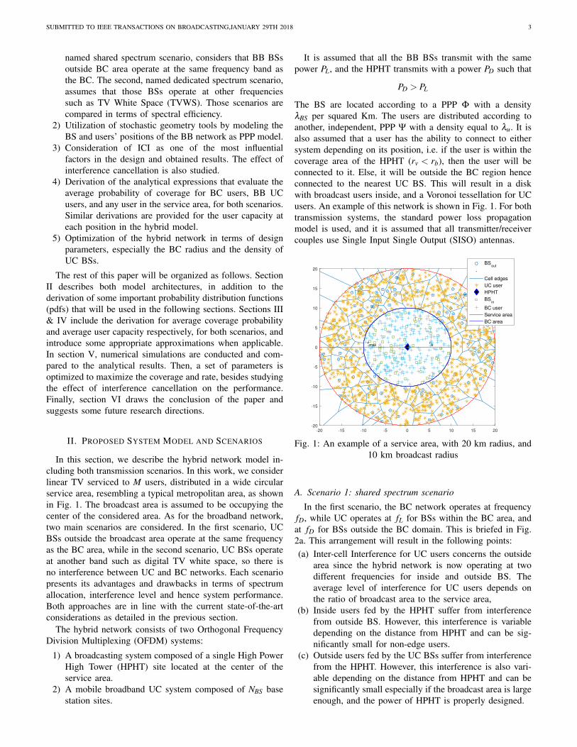


![Scalable WiFi Media Delivery through Adaptive Broadcastspages.cs.wisc.edu/~sdsen/papers/2010medusa.pdfapproaches [23] to improve efficiency. Unicast vs broadcast vs pseudo-broadcast:In](https://static.documents.pub/doc/80x56/60a01a9c7bfcf50bed17fb69/scalable-wifi-media-delivery-through-adaptive-sdsenpapers2010medusapdf-approaches.jpg)
![Towards an LTE hybrid unicast broadcast content delivery ... · The Global Mobile Suppliers Association (GSA) in [6] forecast the market for Long Term Evolution (LTE) broadcast will](https://static.documents.pub/doc/80x56/5b48bba77f8b9a824f8cc855/towards-an-lte-hybrid-unicast-broadcast-content-delivery-the-global-mobile.jpg)
