On the cogrowth of Thompson’s group F * Murray Elder 1 , Andrew Rechnitzer 2 , and Thomas Wong 2 1 School of Mathematical & Physical Sciences, The University of Newcastle 2 Department of Mathematics, University of British Columbia August 18, 2018 Abstract We investigate the cogrowth and distribution of geodesics in R. Thompson’s group F . 1 Introduction In this article we study the cogrowth and distribution of geodesics in Richard Thompson’s group F , in an attempt to decide experimentally whether or not F is amenable. The cogrowth of a finitely generated group G is defined as follows. Suppose S = {a 1 ,...,a k } generates G 1 , and consider the Cayley graph G of (G, S ). Let r n be the number of paths in this graph of length n starting and ending at the identity element — let us call such paths returns. Since we can concatenate any two such paths to get another we have r n r k ≤ r n+k (1) and then by Fekete’s lemma (see, for example, [23]) ρ = lim sup n→∞ r 1 /n n (2) * The first author acknowledges support from ARC projects DP110101104 and FT110100178. The second author thanks NSERC of Canada for financial support. 1 Formally, we consider G as the epimorphic image from the free monoid generated by S ∪ S -1 , rather than S ∪ S -1 as being a subset of G 1 arXiv:1108.1596v2 [math.GR] 9 Oct 2012
Transcript
On the cogrowth of Thompson’s group F ∗
Murray Elder1, Andrew Rechnitzer2, and Thomas Wong2
1School of Mathematical & Physical Sciences, The University of Newcastle2Department of Mathematics, University of British Columbia
August 18, 2018
Abstract
We investigate the cogrowth and distribution of geodesics in R. Thompson’sgroup F .
1 Introduction
In this article we study the cogrowth and distribution of geodesics in RichardThompson’s group F , in an attempt to decide experimentally whether or notF is amenable.
The cogrowth of a finitely generated group G is defined as follows. SupposeS = {a1, . . . , ak} generates G1, and consider the Cayley graph G of (G,S). Letrn be the number of paths in this graph of length n starting and ending at theidentity element — let us call such paths returns. Since we can concatenateany two such paths to get another we have
rnrk ≤ rn+k (1)
and then by Fekete’s lemma (see, for example, [23])
ρ = lim supn→∞
r1/nn (2)
∗The first author acknowledges support from ARC projects DP110101104 and FT110100178.The second author thanks NSERC of Canada for financial support.
1Formally, we consider G as the epimorphic image from the free monoid generated by S ∪ S−1,rather than S ∪ S−1 as being a subset of G
1
arX
iv:1
108.
1596
v2 [
mat
h.G
R]
9 O
ct 2
012
exists. This constant is called the cogrowth for (G,S). Since we considergenerators and their inverses to label distinct edges in G, then ρ ≤ 2k.
The connection between this growth rate and amenability was establishedby Grigorchuk and independently by Cohen:
Theorem 1 ([12, 7]). Let G,S and ρ be as above. G is amenable if and onlyif ρ = 2k.
Let pn be the number of returns of length n on G which do not containimmediate reversals. Again concatenation shows that pn is supermultiplicativeso Fekete’s lemma gives
α = lim supn→∞
p1/nn (3)
exists. In this case since there are 2k(2k−1)n−1 freely reduced words of lengthn in the 2k generators and their inverses, we have α ≤ 2k − 1.
The previous theorem can then be restated as:
Theorem 2 ([12, 7]). Let G,S and α be as above. G is amenable if and onlyif α = 2k − 1.
Note that lim sups are required since, for example, if G has a presentationwhere all relators have even length, the number of returns of odd length (withor without immediate reversals) is 0.
In this article we compute bounds on the cogrowth rates of a number of2-generator groups: Thompson’s group F , the free and free abelian groupson 2 generators, Baumslag-Solitar groups, and various wreath products. Eachof these examples, apart from F , is known to be either amenable or non-amenable. We compare the data obtained for F against these examples, to seewhether F behaves more like an amenable or a non-amenable group.
The question of the amenability of Thompson’s group F has captivatedmany researchers for some time, initially since F has exponential growth butno nonabelian free subgroups, making it a prime candidate for a counterex-ample to von Neumann’s conjecture that a group is non-amenable if and onlyif it contains a nonabelian free subgroup. In 1980 Ol’shanskii constructeda finitely generated non-amenable group with no nonabelian free subgroups[14], and in 1982 Adyan gave further examples [1]. In 2002 Ol’shanskii andSapir constructed finitely presented examples [15]. In spite of these results theamenability or non-amenability of F remains an intensely studied problem.
In the second half of the article we extend our techniques to study thedistribution of geodesic words in Thompson’s group.
This work is in the same spirit as previous papers by Burillo, Cleary andWiest [5], and Arzhantseva, Guba, Lustig, and Preaux [2], who also applied
2
computational techniques to consider the amenability of F . We refer the readerto these papers for more background on Thompson’s group and the problemof deciding its amenability computationally.
The article is organised as follows. In Section 2 we compute rigorous lowerbounds on the cogrowth by computing the dominant eigenvalue of the adja-cency matrix of truncated Cayley graphs. We then extrapolate these boundsto estimate the cogrowth and compare and contrast those extrapolations forF and other groups. In Section 3 we use a weighted random sampling of ran-dom words in the generators to estimate the exponential growth rate of trivialwords in several different groups. As a byproduct we estimate the distributionof geodesic lengths as a function of word-length.
2 Bounding returns and cogrowth
2.1 Bounding the number of returns
Consider the Cayley graph G of some group G with finite generating set — forthe discussion at hand, let us assume that G is generated by two nontrivialelements a, b.
As noted above, an upper bound for the cogrowth ρ is 4. We can computelower bounds for the number of returns, and thus the cogrowth, as follows.
Consider the following sequence of finite connected subgraphs, GN of Nvertices that contain the identity.
Set G1 to be the identity vertex. Record the list of edges incident to G1.Define G2,G3, . . . by appending edges from this list, one at a time. Once thelist is exhausted (so GN = B(1)), repeat the process. It follows that for eachGN there is an R so that B(R) ⊆ GN ⊆ B(R+ 1).
We can then define rN,n be the number of returns of length n in GN . Since
GN ⊂ GN+1, the sequence {rN,n} is supermultiplicative, so ρN = lim supn→∞
r1/nN,n
exists by Fekete’s lemma. Further we must have rn ≥ rN,n and so ρ ≥ ρN .Hence we can bound ρ by computing ρN .
Using the Perron-Frobenius theorem (in one of its many guises — Propo-sition V.7 from [11] for example) the growth rate ρN of such paths on GNis given by the dominant eigenvalue of the corresponding adjacency matrix,provided it is irreducible. We construct GN so that it is connected and so thecorresponding adjacency matrix is be irreducible.
In some cases we can also demonstrate that the adjacency matrix is aperi-odic, which implies that the dominant eigenvalue is simple and dominates allother eigenvalues. This also implies that the corresponding generating function
3
∑pN,nz
n has a simple pole at the reciprocal of that eigenvalue. Unfortunatelymany of the matrices we study are not aperiodic, but they do have period 2.
Perhaps the easiest way to prove that the matrix is aperiodic is to showthe existence of two circuits of relatively prime length (see chapter V.5 in [11]for example). In order to show that a matrix has period 2 it suffices (providingthe matrix is finite) to show that if there is a path of length k between anytwo nodes, then there is a path of length k + 2` between those two nodes forany `.
It follows that the adjacency matrix for GN is aperiodic whenever the groupG has a presentation with an odd length relator (since aa−1 and the odd lengthrelator form circuits of relatively prime lengths) and if all relators have evenlength, the matrix has period 2 (since a path of length k can be made into apath of length k + 2` by inserting (aa−1)`).
In particular we have that subgraphs of Baumslag-Solitar groups BS(p, q)with p + q odd are aperiodic, while subgraphs of BS(p, q) with p + q even,Thompson’s group F , Z2, Z o Z and F2 (the free group on 2 generators), allwith the usual generating sets, have period 2.
Since all of above groups except Z2 grow exponentially, and B(R) ⊆ GN ⊆B(R + 1), then the radius of GN is O(logN). In the case of Z2 the radius ofGN is O(
√N)
We used this method to compute ρN for a selection of groups. However,we found significantly better bounds by considering only freely reduced words,i.e. paths that did not contain immediate reversals, essentially since there isless to count.
2.2 Bounding the cogrowth
Let pn be the number of returns of length n on G which do not contain imme-diate reversals. We similarly define pN,n to be similar paths on the subgraphGN . Again we define the exponential growth of these quantities by
α = lim supn→∞
p1/nn αN = lim sup
n→∞p1/nN,n
and α ≥ αN .In this case, we cannot now simply concatenate two freely reduced paths to
obtain another freely reduced path since it may create an immediate reversal.Thus we do not have similar supermultiplicative relations. We can, however,relate rn to pn and ρ to α using the following result of Kouksov [13] which wehave specialised to the case of 2 generator groups.
4
Lemma 3. (from [13]) Let R(z) =∑rnz
n and C(z) =∑pnz
n be the gener-ating functions of returns and freely reduced returns respectively. Then
C(z) =1− z2
1 + 3z2R
(z
1 + 3z2
)and equivalently
R(z) =−1 + 2
√1− 12z2
1− 16z2C
(1−√
1− 12z2
6z
).
A careful generating function argument gives the second equation (and thefirst is simply its inverse). Consider any freely reduced returning path; it canbe mapped to an infinite set of returning paths by replacing each edge s byany returning path in the free group on 2 generators that does start with s−1.At the level of generating functions, this is exactly the substitution
z 7→ 1−√
1− 12z2
6z.
A very general result for generating functions then links the dominantsingularity of R(z) to the value of ρ:
Theorem 4. ([11], page 240.) If f(z) is analytic at 0 and ρ is the modulus ofa singularity nearest to the origin, then the coefficient fn = [zn]f(z) satisfies:
lim supn→∞
|fn|−1/n = ρ
Combining these two results (and using the positivity of rn, pn) we obtain
Corollary 5. The constants ρ and α are related by
ρ =α2 + 3
α
Further if β is a lower bound for α, then β′ =β2 + 3
βis an lower bound for ρ.
We are unable to prove a similar exact relationship between ρN and αN ,but we do have the following bound:
Lemma 6. For a fixed value of N we have ρN ≤α2N + 3
αN.
Proof. Consider the generating functions of returns and freely reduced returnson Gn.
RN (z) =∑n≥0
rN,nzn CN (z) =
∑n≥0
pN,nzn
5
It suffices to show that
CN (z) ≥ 1− z2
1 + 3z2RN
(z
1 + 3z2
)or equivalently
RN (z) ≤ −1 + 2√
1− 12z2
1− 16z2CN
(1−√
1− 12z2
6z
)
within the respective radii of convergence. Let ω be any freely reduced re-turning path of length k in GN — this path contributes zk to the generating
function CN (z). The substitution z 7→ 1−√
1− 12z2
6zmaps ω to an infinite
set of non-reduced returning paths by replacing each edge with freely reducedwords from F2. Some of the resulting words will lie entirely within GN and sobe enumerated by the generating function RN (z). However an infinite numberof these words will not be contained in GN . These words are enumerated by
−1 + 2√
1− 12z2
1− 16z2CN
(1−√
1− 12z2
6z
)
but not by RN (z). Thus the inequality follows.
To compute αN we relate it to the dominant eigenvalue of an adjacencymatrix. Unfortunately there is no simple way to reuse the adjacency matrixof GN , in order to enumerate paths without immediate reversal. Instead weconstruct a new graph HN which encodes freely reduced paths in G as follows:HN has N vertices labeled by pairs (1,−) or (g, s) where g ∈ G and s ∈ S.The vertex (1,−) corresponds to being at the identity vertex of G, and (g, s)to being at the group element g ∈ G after having just read a letter s. Theedges of HN are
E(HN ) = {((g, s), (h, t)) ∈ (V (HN ))2 | h = gt and st 6= 1} (4)
So a path (1,−), (g1, s1), (g2, s2), . . . (gk, sk) corresponds to a path in G startingat 1 with g1 = s1, g2 = s1s2, . . . gk = s1s2 . . . sk a freely reduced word.
We construct HN using a breadth-first search similar to the constructionof GN , starting with H1 = (1,−) and appending vertices one at a time so that{g ∈ G | (g, s) ∈ HN} lies between two balls of a given radius. It follows thatHN is necessarily connected, and the corresponding adjacency matrices areirreducible.
We then compute the growth rate of paths (and so freely reduced returns)on HN by computing the dominant eigenvalue of the corresponding adjacencymatrix.
6
2.3 Exact lower bounds
Since each node of GN has outdegree at most 4 and those of the HN excluding(1,−) have outdegree at most 3 (vertices on the boundary may have smallerdegree) the corresponding adjacency matrices are sparse. We found that thepower method and Rayleigh quotients (see [20] for example) converged veryquickly to the dominant eigenvalue and so the growth rate.
We constructed GN and HN for many different values of N ranging between102 and 107. Our calculations on Thompson’s group F as well as the Baumslag-Solitar groups BS(2, 2), BS(2, 3) and BS(3, 5), yielded the following result.
Theorem 7. The following are exact lower bounds on the cogrowth, α, of theindicated groups.
Note that all of these bounds were computed using information from HNand Corollary 5. We observed that the bounds obtained from GN were worse— typically differing in the second or third significant digit. We also note thatthe above result for BS(2, 3) is improves on a result in [9] (the preprint waswithdrawn by the authors since it contained an error).
These computations were done on a desktop computer using about 4Gb ofmemory. It should be noted that while our techniques require both exponentialtime and memory, it was memory that was the constraining factor. We didimplement some simple space-saving methods. Perhaps the most effective ofthese was to store elements as geodesic words in the generators rather thanas their more standard normal forms (eg tree-pairs for Thompson’s group orwords in the normal form implied by Britton’s lemma for the Baumslag-Solitargroups). These geodesic words could then be stored as bit-strings rather thanASCII strings. We believe that by running these computations on a computerwith more memory we could improve the bounds, but the returns are certainlydiminishing.
2.4 Extrapolation and comparison
The results of the previous section can be extended by considering the sequenceof lower bounds αN and using simple numerical methods to extrapolate them
7
to N → ∞. This required only minimal changes to our computations; aftercomputing the adjacency matrix of HN for the maximal value of N , we com-puted the dominant eigenvalue of submatrices. The corresponding estimate ofthe eigenvector was then used as an initial vector for estimating the eigenvalueof the next submatrix. This meant that we could compute a sequence of lowerbounds in not much more time than it took to compute our best bounds.
In Figure 1 we have plotted αN against 1/logN for three non-amenableBaumslag-Solitar groups and F . We found that this gave approximately linear
Figure 1: A plot of cogrowth lower bounds αN against 1/logN. We see that thegroups that known to be non-amenable are converging to numbers strictly below3. The Thompson’s group sequence has a clear upward inflection (as N → ∞ or1/logN → 0) and so it is difficult to estimate whether the limit is 3 or less than 3.
plots and so this suggests that
αN ≈ α∞ − λ/logN.
Since αN is a monotonically increasing sequence and is bounded above by 3,we have that αN → α∞ exists. Unfortunately we cannot prove that α∞ = α,but certainly α∞ ≤ α.
Note that the curves terminate at N = 107 but start at different N -values.This is because the graphs GN do not contain freely-reduced loops for small
8
values of N . The smallest value of N for which GN contains a freely reducedloop depends on the length of the relations of the group and on the details ofthe breadth-first search used to construct the graph.
One can observe that the Baumslag-Solitar groups all seem to behave sim-ilarly and that the sequences of bounds are clearly converging to constantsstrictly less than 3. This is completely consistent with the non-amenability ofthese groups. Thompson’s group behaves quite differently — in particular wesee that the curve has some upward inflection (as x→ 0) and it makes it veryunclear as to whether or not α∞ converges to 3 or below 3.
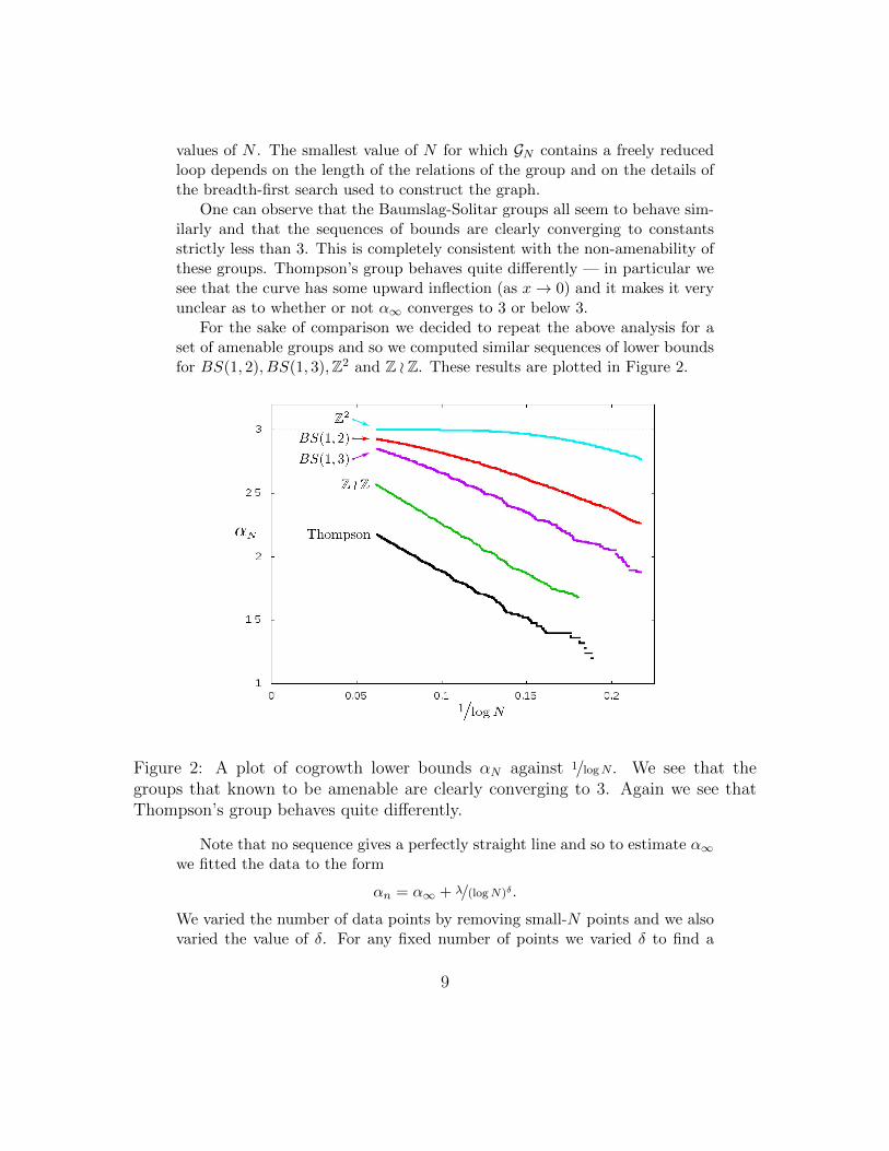
For the sake of comparison we decided to repeat the above analysis for aset of amenable groups and so we computed similar sequences of lower boundsfor BS(1, 2), BS(1, 3),Z2 and Z o Z. These results are plotted in Figure 2.
Figure 2: A plot of cogrowth lower bounds αN against 1/logN. We see that thegroups that known to be amenable are clearly converging to 3. Again we see thatThompson’s group behaves quite differently.
Note that no sequence gives a perfectly straight line and so to estimate α∞we fitted the data to the form
αn = α∞ + λ/(logN)δ.
We varied the number of data points by removing small-N points and we alsovaried the value of δ. For any fixed number of points we varied δ to find a
9
value that minimised the R2 statistic. This gives an “optimal” value of α∞and λ.
For some groups, we found that these optimal values were quite sensitive tochanges in δ, while other groups were quite robust. To include some measureof this systematic error we moved δ through a range of values so that the R2
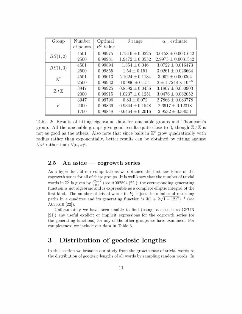
statistic was allowed to move to 5% below its optimal value. These results aresummarised in Tables 1 and 2.
The results for all the groups except Thompson’s group are as one mightexpect — the amenable groups all give estimates of α∞ close to 3, and thenon-amenable groups give α∞ < 3. Hence it would appear as though this tech-nique is a reasonable test to differentiate amenable and non-amenable groups.Unfortunately it is not sufficiently sensitive to determine the amenability ofThompson’s group. In particular we find that the results are too sensitive tovariations in δ and to removal of low-N data points. A possible reason for thisatypical behaviour is the presence of nested wreath products which convergevery slowly to their asymptotic behaviour.
Because of this, we turn to numerical methods based on random samplingand approximate enumeration.
Group Number Optimal δ range α∞ estimateof points R2 Value
Table 1: Results of fitting eigenvalue data for non-amenable groups and Thompson’sgroup. The Baumslag-Solitar groups all give good results, but Thompson’s groupdoes not. There is some upward drift in the estimate of α∞ as one cuts out small Ndata, but at the same time the error in the estimates blows up.
10
Group Number Optimal δ range α∞ estimateof points R2 Value
Table 2: Results of fitting eigenvalue data for amenable groups and Thompson’sgroup. All the amenable groups give good results quite close to 3, though Z o Z isnot as good as the others. Also note that since balls in Z2 grow quadratically withradius rather than exponentially, better results can be obtained by fitting against1/Nδ rather than 1/(logN)δ.
2.5 An aside — cogrowth series
As a byproduct of our computations we obtained the first few terms of thecogrowth series for all of these groups. It is well know that the number of trivial
words in Z2 is given by(2nn
)2(see A002894 [22]); the corresponding generating
function is not algebraic and is expressible as a complete elliptic integral of thefirst kind. The number of trivial words in F2 is just the number of returningpaths in a quadtree and its generating function is 3(1 + 2
√1− 12z2)−1 (see
A035610 [22]).Unfortunately we have been unable to find (using tools such as GFUN
[21]) any useful explicit or implicit expressions for the cogrowth series (orthe generating functions) for any of the other groups we have examined. Forcompleteness we include our data in Table 3.
3 Distribution of geodesic lengths
In this section we broaden our study from the growth rate of trivial words tothe distribution of geodesic lengths of all words by sampling random words. In
Table 3: The first few terms of the cogrowth series C(z) for various groups, i.e. thenumber of freely reduced words equivalent to the identity. The first few terms of thereturns series R(z) can be obtained from the above using Lemma 3.
previous work of Burillo et al [5], random words in Thompson’s group F weresampled using simple sampling; words were grown by appending generatorsone-by-one uniformly at random. Those authors observed only very trivialwords and so then sampled uniformly at random from a subset of those words,namely the set of words with balanced numbers of each generator and theirinverses. Again, very few trivial words were observed. Indeed if Thompson’sgroup is non-amenable, the probability of observing a trivial word using simplesampling will decay exponentially quickly.
We will proceed along a similar line but using a more powerful random sam-pling method based on flat-histogram ideas used in the FlatPERM algorithm
12
[17, 18]. Each sample word is grown in a similar manner to simple sampling— append one generator at a time chosen uniformly at random. The weight ofa word of n symbols is simply 1, so that the total weight of all possible wordsat any given length is just 4n. As the word grows we keep track of its geodesiclength. We now deviate from simple sampling by “pruning” and “enriching”the words.
Consider a word of length n, geodesic length ` and weight W . If we have“too many” samples of such words, then with probability 1/2 prune the currentsample or otherwise continue to grow the current sample but with weight 2W .Similarly if we have “too few” samples of the current length and geodesiclength, then enrich by making 2 copies of the current word and then growing asample from both each with weight W/2. Of course, one is free to play aroundwith the precise meaning of “too few” or “too many”. We refer the reader to[17, 18] for more details on the implementation of this algorithm. The meanweight (multiplied by 4n) of all samples of length n and geodesic length `, cn,`,is then an estimate of the number of such words.
In order to run the above algorithm we need to be able to compute thegeodesic length of the element generated by a given random word. Computinggeodesic lengths from a normal form is, in general, a very difficult problem andremains stubbornly unsolved for many interesting groups, such as BS(2, 3).Because of this we restrict our studies to Thompson’s group and a number ofdifferent wreath products.
• Thompson’s group — a method for computing the geodesic length of anelement from its tree-pair representation was first given by Fordham [4],though we found it easier to implement the method of Belk and Brown[3].
• Wreath products — we use the results of [6] to find the geodesic lengthsin Z o Z, Z o (Z o Z) and Z o F2.
We note that the geodesic problem for Baumslag-Solitar groups has recentlybeen solved in the cases BS(1, n) [10] and BS(n, kn) [8], but we have notimplemented these approaches.
3.1 Distributions
We used the random sampling algorithm described above to estimate the dis-tribution of geodesic lengths in Thompson’s group F , as well as Z oZ, Z oF2 andZ o (Z oZ). Each run took approximately 1 day on a modest desktop computer.To visualise the results, we started by normalising the data by dividing by thetotal number of words (i.e. 4n or 6n). The resulting peak-heights still decay
13
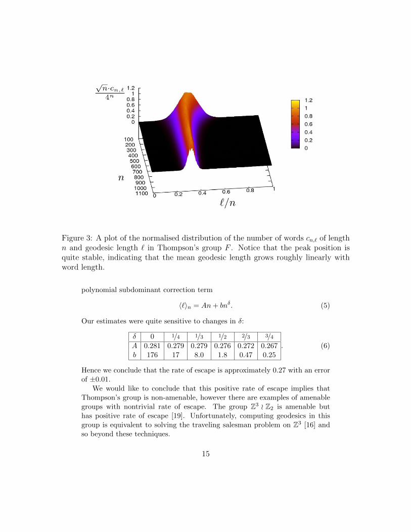
with length, and we found that multiplying by√n compensated for this. The
normalised distributions are plotted in Figures 3, 4 and 5.In each case we see similar behaviour. At short word lengths (i.e. small n)
the distribution of geodesic lengths is quite wide, but settles to what appearsto be a bell-shaped distribution at moderate lengths. This suggests that thegeodesic length has an approximately Gaussian distribution about the meanlength and that the tails of the distribution are exponentially suppressed. Thisalso explains why the normalising factor of
√n works well.
If this is indeed the case, then we expect that trivial words, having geodesiclength zero, will be exponentially fewer than 4n — implying that Thompson’sgroup is non-amenable. Unfortunately things cannot be so simple, because thesame reasoning would imply that Z o Z is non-amenable.
One obvious difference between the graphs is the movement of the peakof the distribution, that is the rate of growth of the mean geodesic length.It is clear that the mean geodesic length of Z o F2 grows linearly, and so thegroup has a nontrivial rate of escape — exactly as one would expect of a non-amenable group. Similarly we see that the mean geodesic lengths of the otherwreath products grow sublinearly, so their rates of escape are zero. When weexamine the movement of the peak of Thompson’s group’s distribution, thingsare less clear; the mean geodesic length appears to be very nearly linear.
Estimating the mean geodesic length for Thompson’s group was substan-tially easier. We constructed 212 random words of length 216. As each wordwas constructed generator-by-generator, the geodesic length was computedand added to our statistics. So while there is correlation between the geodesiclengths at different word lengths within a given sample, there is no correla-tion between samples. This took approximately 3 days on a modest desktopcomputer. Our data is plotted in Figure 6.
We assume that the mean geodesic length grows as nν . Linear regressionon a log-log plot estimates ν ≈ 0.98. Further, if we fit a moving “window”,we find that the local estimates of ν increase as the positioning of the windowincreases. This strongly suggests that the mean geodesic length grows linearly.
To test linearity further, we generated a small number words of length220 = 1048576. It took approximately 1 hour to generate each word andcompute the corresponding geodesic length, so this was too slow to generatemeaningful statistics. In each case we observed that the ratio /n appearedto converge to approximately 0.28. Of course, this does not preclude moreexotic sublinear behaviour such as nν(log n)θ. Such logarithmic correctionsare extremely difficult to detect or rule out.
We now estimate the rate of escape by assuming linear growth with a
14
Figure 3: A plot of the normalised distribution of the number of words cn,` of lengthn and geodesic length ` in Thompson’s group F . Notice that the peak position isquite stable, indicating that the mean geodesic length grows roughly linearly withword length.
polynomial subdominant correction term
〈`〉n = An+ bnδ. (5)
Our estimates were quite sensitive to changes in δ:
Hence we conclude that the rate of escape is approximately 0.27 with an errorof ±0.01.
We would like to conclude that this positive rate of escape implies thatThompson’s group is non-amenable, however there are examples of amenablegroups with nontrivial rate of escape. The group Z3 o Z2 is amenable buthas positive rate of escape [19]. Unfortunately, computing geodesics in thisgroup is equivalent to solving the traveling salesman problem on Z3 [16] andso beyond these techniques.
15
Figure 4: A plot of the normalised distribution of the number of words cn,` of lengthn and geodesic length ` in Z o Z. Observe that the peak position is clearly movingtowards the left of the plot suggesting that the mean geodesic length grows sublin-early.
4 Conclusions
We have computed exact lower bounds on the cogrowth of several groupsincluding Thompson’s group F . In particular, the cogrowth (α) of Thompson’sgroup must be greater than 2.17329. By extrapolating the sequences of lowerbounds we see that the bounds for the amenable groups clearly converge to3, while those of the non-amenable groups converge to numbers strictly lessthan 3. Thompson’s group appears to behave quite differently from the othergroups we examined. Our extrapolations do not give clear results, thoughperhaps they point towards non-amenability.
To further probe this group we used flat histogram methods to estimatethe distribution of geodesic lengths in random words. The data suggeststhat geodesic lengths have an approximately Gaussian distribution about theirmean length. Similar Gaussian distributions were observed for other groups,both amenable and non-amenable.
The mean geodesic length of the amenable groups studied grow sublinearly,
16
Figure 5: Plot of the normalised distribution of the number of words cn,` of length nand geodesic length ` in Z oF2 (left) and Z o (Z oZ) (right). Observe that the peak isquite stable in the left-hand plot indicating the mean geodesic length is linear, whilethe right-hand plot the peak shows clear a left drift indicating that the geodesicsgrow sublinearly.
Figure 6: Plot of the mean geodesic length divided by nν ; for ν = 0.98, 0.99 and 1.This data strongly suggests that Thompson’s group has a nontrivial rate of escape.Note that the statistical error was smaller than the symbols used.
while those of ZoF2 and Thompson’s group are observed to grow linearly. Usingsimple sampling we estimate that the mean geodesic length of Thompson’s
17
group does indeed grow linearly and that the rate of escape is 0.27± 0.01.
5 Acknowledgments
We thank the anonymous reviewers for their helpful comments, and WestGridfor computer support.
References
[1] S. I. Adyan. Random walks on free periodic groups. Izv. Akad. Nauk SSSRSer. Mat., 46(6):1139–1149, 1343, 1982.
[2] G.N. Arzhantseva, V.S. Guba, M. Lustig, J. Preaux. Testing Cayley graphdensities. (Tester les densites de graphes de Cayley.) (French) Ann. Math.Blaise Pascal 15(2):233–286, 2008.
[3] J.M. Belk and K.S. Brown. Forest diagrams for elements of Thompson’sgroup F . International Journal of Algebra and Computation, 15(6):815–850, 2005.
[4] S. Blake Fordham. Minimal length elements of Thompson’s group F. Ge-ometriae Dedicata, 99(1):179–220, 2003.
[5] Jose Burillo, Sean Cleary, and Bert Wiest. Computational explorationsin Thompson’s group F . In Geometric group theory, Trends Math., pages21–35. Birkhauser, Basel, 2007.
[6] S. Cleary and J. Taback. Metric properties of the lamplighter group asan automata group. Geometric Methods In Group Theory: AMS SpecialSession Geometric Group Theory, October 5-6, 2002, Northeastern Uni-versity, Boston, Massachusetts: Special Session At The First Joint Mee,372:207, 2005.
[7] Joel M. Cohen. Cogrowth and amenability of discrete groups. J. Funct.Anal., 48(3):301–309, 1982.
[8] V. Diekert and J. Laun. On computing geodesics in Baumslag-Solitargroups. Internat. J. Algebra Comput., 21(1–2):119–145, 2011.
[9] K. Dykema and D. Redelmeier. Lower bounds for the spectral radiiof adjacency operators on Baumslag-Solitar groups. Arxiv preprintarXiv:1006.0556, 2010.
[10] M. Elder. A linear-time algorithm to compute geodesics in solvableBaumslag-Solitar groups. Illinois J. Math., 54(1):109–128, 2010.
[11] P. Flajolet and R. Sedgewick. Analytic combinatorics. Cambridge UnivPr, 2009.
[12] R. I. Grigorchuk. Symmetrical random walks on discrete groups. InMulticomponent random systems, volume 6 of Adv. Probab. Related Topics,pages 285–325. Dekker, New York, 1980.
[13] D. Kouksov. On rationality of the cogrowth series. Proceedings of theAmerican Mathematical Society, 126(10):2845–2847, 1998.
[14] Alexander Yu. Ol’shanskii. On the question of the existence of an invariantmean on a group. Uspekhi Mat. Nauk, 35(4(214)):199–200, 1980.
[15] Alexander Yu. Ol’shanskii and Mark V. Sapir. Non-amenable finitelypresented torsion-by-cyclic groups. Publ. Math. Inst. Hautes Etudes Sci.,No. 96:43–169 (2003), 2002.
[16] Walter Parry. Growth series of some wreath products. Trans. Amer.Math. Soc., 331(2):751–759, 1992.
[17] T. Prellberg and J. Krawczyk. Flat histogram version of the pruned andenriched Rosenbluth method. Physical review letters, 92(12):120602, 2004.
[18] T. Prellberg, J. Krawczyk, and A. Rechnitzer. Polymer Simulations witha Flat Histogram Stochastic Growth Algorithm. In Computer simulationstudies in condensed-matter physics XVI: proceedings of the seventeenthworkshop, Athens, GA, USA, February 16-20, 2004, page 122. SpringerVerlag, 2006.
[19] David Revelle. Rate of escape of random walks on wreath products andrelated groups. Ann. Probab., 31(4):1917–1934, 2003.
[20] Y. Saad. Iterative methods for sparse linear systems. Society for IndustrialMathematics, 2003.
[21] Bruno Salvy and Paul Zimmermann. Gfun: a Maple package for themanipulation of generating and holonomic functions in one variable. ACMTransactions on Mathematical Software, 20(2):163–177, 1994.
[22] N. J. A. Sloane (ed). The On-Line Encyclopedia of Integer Sequences.published electronically at http://oeis.org/.
[23] J.H. van Lint and R.M. Wilson. A course in combinatorics. CambridgeUniv Pr, 2001.