20 On the Complexity of Traffic Traces and Implications CHEN AVIN, School of Electrical and Computer Engineering, Ben Gurion University of the Negev, Israel MANYA GHOBADI, Computer Science and Artificial Intelligence Laboratory, MIT, USA CHEN GRINER, School of Electrical and Computer Engineering, Ben Gurion University of the Negev, Israel STEFAN SCHMID, Faculty of Computer Science, University of Vienna, Austria This paper presents a systematic approach to identify and quantify the types of structures featured by packet traces in communication networks. Our approach leverages an information-theoretic methodology, based on iterative randomization and compression of the packet trace, which allows us to systematically remove and measure dimensions of structure in the trace. In particular, we introduce the notion of trace complexity which approximates the entropy rate of a packet trace. Considering several real-world traces, we show that trace complexity can provide unique insights into the characteristics of various applications. Based on our approach, we also propose a traffic generator model able to produce a synthetic trace that matches the complexity levels of its corresponding real-world trace. Using a case study in the context of datacenters, we show that insights into the structure of packet traces can lead to improved demand-aware network designs: datacenter topologies that are optimized for specific traffic patterns. CCS Concepts: • Networks → Network performance evaluation; Network algorithms; Data center networks;• Mathematics of computing → Information theory; Additional Key Words and Phrases: trace complexity, self-adjusting networks, entropy rate, compress, com- plexity map, data centers ACM Reference Format: Chen Avin, Manya Ghobadi, Chen Griner, and Stefan Schmid. 2020. On the Complexity of Traffic Traces and Implications. Proc. ACM Meas. Anal. Comput. Syst. 4, 1, Article 20 (March 2020), 29 pages. https://doi.org/10. 1145/3379486 1 INTRODUCTION Packet traces collected from networking applications, such as datacenter traffic, have been shown to feature much structure: datacenter traffic matrices are sparse and skewed [16, 39], exhibit locality [21], and are bursty [77, 83]. In other words, packet traces from real world applications are far from arbitrary or random. Motivated by the existence of such structure, the networking community is currently putting effort into designing protocols and algorithms to optimize different layers of the networking stack to leverage the traffic structure. These efforts include learning-based traffic engineering [70] and video streaming [55], demand-aware and self-adjusting reconfigurable optical networks [14, 39, 42, 57], or self-driving networks [69, 76]. For instance, many network optimizations exploit the presence of elephant flows [6]. However, the available structure can differ significantly across applications, and we currently lack a unified approach to measure the structure in traffic traces in a systematic manner, accounting for both non-temporal structures (e.g., how skewed the traffic matrices are) and temporal structures (e.g., how bursty traffic is). The quantification of trace structures and their locality can be very Authors appear in alphabetical order. Research conducted as part of Chen Griner’s thesis. Authors’ addresses: Chen Avin, School of Electrical and Computer Engineering, Ben Gurion University of the Negev, Beer Sheva, Israel, [email protected]; Manya Ghobadi, Computer Science and Artificial Intelligence Laboratory, MIT, Boston, USA, [email protected]; Chen Griner, School of Electrical and Computer Engineering, Ben Gurion University of the Negev, Beer Sheva, Israel, [email protected]; Stefan Schmid, Faculty of Computer Science, University of Vienna, Vienna, Austria, [email protected]. Proc. ACM Meas. Anal. Comput. Syst., Vol. 4, No. 1, Article 20. Publication date: March 2020.
Transcript
20
On the Complexity of Traffic Traces and Implications
CHEN AVIN, School of Electrical and Computer Engineering, Ben Gurion University of the Negev, Israel
MANYA GHOBADI, Computer Science and Artificial Intelligence Laboratory, MIT, USA
CHEN GRINER, School of Electrical and Computer Engineering, Ben Gurion University of the Negev,
Israel
STEFAN SCHMID, Faculty of Computer Science, University of Vienna, Austria
This paper presents a systematic approach to identify and quantify the types of structures featured by packet
traces in communication networks. Our approach leverages an information-theoretic methodology, based on
iterative randomization and compression of the packet trace, which allows us to systematically remove and
measure dimensions of structure in the trace. In particular, we introduce the notion of trace complexity which
approximates the entropy rate of a packet trace. Considering several real-world traces, we show that trace
complexity can provide unique insights into the characteristics of various applications. Based on our approach,
we also propose a traffic generator model able to produce a synthetic trace that matches the complexity levels
of its corresponding real-world trace. Using a case study in the context of datacenters, we show that insights
into the structure of packet traces can lead to improved demand-aware network designs: datacenter topologies
that are optimized for specific traffic patterns.
CCS Concepts: • Networks → Network performance evaluation; Network algorithms; Data centernetworks; • Mathematics of computing→ Information theory;
Additional Key Words and Phrases: trace complexity, self-adjusting networks, entropy rate, compress, com-
plexity map, data centers
ACM Reference Format:Chen Avin, Manya Ghobadi, Chen Griner, and Stefan Schmid. 2020. On the Complexity of Traffic Traces and
or self-driving networks [69, 76]. For instance, many network optimizations exploit the presence of
elephant flows [6].
However, the available structure can differ significantly across applications, and we currently
lack a unified approach to measure the structure in traffic traces in a systematic manner, accounting
for both non-temporal structures (e.g., how skewed the traffic matrices are) and temporal structures(e.g., how bursty traffic is). The quantification of trace structures and their locality can be very
Authors appear in alphabetical order. Research conducted as part of Chen Griner’s thesis.
Authors’ addresses: Chen Avin, School of Electrical and Computer Engineering, Ben Gurion University of the Negev, Beer
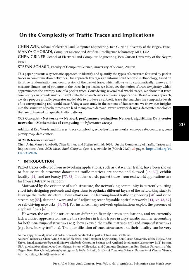
(a) Temporal structure in the original traceSource GPU
Destina
tion G
PU
(c) TM of (a)&(b)
TimeEntries in the trace are shown in the order of appearance.
(b) Shuffling the entries in (a) removes the temporal structure
(d) A trace with lowest structure corresponding to (a)
(e) A trace with highest temporal structure corresponding to (d) (f) TM of (d)&(e)
Source GPU
Destina
tion G
PU
Fig. 1. Visualization of temporal and non-temporal structure in a machine learning workload. The workload istraining a VGG [26] neural network across four GPUs. Each of the different colors inside the traffic matrix (TM)represents a single source-destination pair.
useful; it can shed light on the potential of traffic-aware optimization, and facilitate traffic modeling,
benchmarking, and synthesis; these are otherwise difficult to achieve, given the limited amount of
traffic data available to researchers today.
Let us illustrate the temporal and non-temporal structures available in a traffic trace with an
example. Consider a packet trace from a Machine Learning (ML) application based on a popular
convolutional neural network training job, with four GPUs. Figure 1(a) visualizes the trace where
each packet in the trace is represented by a unique color corresponding to its (source, destination)-
GPU pair. The figure highlights the temporal structure of the trace: the sequence of colors is far fromrandom. Rather, a pattern is revealed, where certain colors are more frequent in some intervals than
in others. For comparison, Figure 1(b) shows the same trace, but randomizes the order of the entries
in the trace: the randomization removes the temporal structure observed in Figure 1(a). Intuitively,
the trace in Figure 1(a) has more temporal structure than the trace in Figure 1(b). However, the
frequency distribution of the two traces is the same: summing up the entries over the entire trace
file results in the same traffic matrix (TM), shown in Figure 1(c).
The resulting traffic matrix shows structure as well. In this case the traffic matrix is skewed,i.e., some GPU pairs communicate more frequently than others. That is, the traffic matrix loses
information about temporal differences, and it features a non-temporal structure. For comparative
purposes, consider two synthetic traces shown in Figures 1(d) and (e). Trace (d) is generated
uniformly and random and has the least temporal structure compared to (a), while trace (e) is burstyand built from consecutive source-destination requests, and hence has the most temporal structure.
Similarly, the traffic matrix in Figure 1(f) captures the non-temporal structure in both (d) and (e),
but not the temporal structure. The traffic matrix is almost uniform, and hence has less structure
than (c).
While the different temporal and non-temporal structures in the above traces are obvious and
intuitive, we currently lack a systematic approach to measure and quantify them. Capturing the
structure of various packet traces is inherently a difficult task: packet traces are often created with
an ad-hoc number of nodes and produce an unknown amount of load on the network. In fact, some
traces are produced using simulation tools to illustrate congestion [6] while others are sampled
from production datacenters [16, 63, 77]. Such disparity in the environment in which the trace
Proc. ACM Meas. Anal. Comput. Syst., Vol. 4, No. 1, Article 20. Publication date: March 2020.
On the Complexity of Traffic Traces and Implications 20:3
DB
WEB
HADHPC
pfabML
Uniform
Skewed
Bursty
Skewed& Bursty
0.3 0.4 0.5 0.6 0.7 0.8 0.9 1.0.3
0.4
0.5
0.6
0.7
0.8
0.9
1.
Temporal complexity
Non
-temporalcomplexity
Fig. 2. The complexity map of six real traces (colored circles) and four reference points (grey circles at thecorners). HAD, WEB, and DB refer to Facebook’s Hadoop, web, and database traces [63]. Two correspondingtraces from Figure 1, traces (a) and (d), are shown above the map. More details about the traces are providedin Table 2.
is captured hinders the reproduction of the structural patterns hidden in the trace. We also lack
methods to synthesize traces with similar structures.
This paper takes the first steps to close this gap. In particular, we propose an approach to quantify
the amount of temporal and non-temporal structure in traffic traces using the information theory’s
measure of entropy [65]. Since the term entropy is defined for random variables, as opposed to a
sequence of individual communication requests in a packet trace, in this paper, we will use the more
general term “complexity” [82] to quantify the structure in a packet trace. In particular, we will
refer to the complexity of a trace as the trace complexity. We will also provide a traffic generation
model to produce synthetic traces that match the complexity of a given real world trace. Intuitively,
a packet trace with low entropy has low complexity: it contains little information, and the sequence
behavior is more predictable [35]; hence we say that it has high structure. Our goal is to enable
a unified mechanism to compare the structure pattern in traces, irrespective of the number of
nodes and the exact packet arrival times. While prior work focused on providing distributions for
flow (or packet) inter-arrival times and sizes [5, 16, 77], we intentionally replace the packet arrival
times with the order of arrival to introduce a degree-of-freedom that enables us to compare traces
captured in widely different settings.
Our approach allows us to chart, what we call, a complexity map of individual traffic traces.
More specifically, we map each traffic trace to a two-dimensional graph indicating the amount of
temporal and non-temporal complexity that is present in a trace. Figure 2 shows an example of
this map. While details will follow later, the map allows us to locate different workloads according
to their temporal complexity (x-axis) and their non-temporal complexity (y-axis). The size of the
circle represents the total complexity, both temporal and non-temporal. A uniform trace without
Proc. ACM Meas. Anal. Comput. Syst., Vol. 4, No. 1, Article 20. Publication date: March 2020.
20:4 Avin et al.
any temporal nor non-temporal structure (like the trace in Figure 1(d) that is shown again above
the map) will be located on the upper right corner x = 1 and y = 1. A trace that is both skewedand bursty has both temporal and non-temporal complexity that are significantly lower than a
uniform trace. The trace of our ML example in Figure 1(a) (shown again above the map) is such an
example and is denoted on the map by the yellow circle. A skewed trace (like the trace in Figure 1(b))
does not have any temporal structure, so its temporal complexity is maximal: the trace will be
located at x = 1. However, as this trace contains non-temporal structure, i.e., is skewed (recall the
matrix in Figure 1(c)), its y-value may be lower. Given this intuition, we indicate in the figure five
additional workloads: three Facebook datacenter workloads (DB, WEB, HAD), a high-performance
computing workload (HPC), and a synthetic pFabric [7] workload (pFab). They all provide different
complexities, as our approach highlights. We will provide more details on these workloads and on
how the complexity map is computed later in the paper.
The main contribution of this paper is a systematic information-theoretic approach to identify
and quantify the types of structures (e.g., temporal and non-temporal) featured by packet traces in
communication networks. Our approach uses iterative randomization and compression of the packet
trace: we iteratively remove and measure dimensions of structure in the trace. We demonstrate an
application of our approach in a case study: the design of demand-aware datacenter topologies. In
particular, we show that insights into the structure of packet traces can lead to improved network
designs that are optimized toward specific traffic patterns. We further present a simple yet powerful
model to generate traffic traces that match the complexity of production-level traces, also allowing
us to derive theoretical properties of the complexity for stationary processes.
As an empirical contribution, we shed light on the different complexities of 17 different traces,
shown in Table 2, including production-level traces (from Facebook [63] and High Performance
load, as well as synthetically generated traces as reference points (for uniform, skewed, and bursty
traffic patterns). We offer several empirical insights into these traces, e.g., on the application-specific
structures, on the differences between the structures available at rack-level versus IP-level, or on
the differences between the structures of sources versus destinations.
As a contribution to the networking community and in order to facilitate future research in the
area, we made available a website trace-collection.net with more resources and data related to this
paper. We plan to extend this website further in the future.
The rest of this paper is organized as follows. We present our approach in §2, and report on
empirical results in §3. We introduce our model in §4 and discuss our case study in §5. In §6 we
extend our initial complexities. After reviewing related work in §7, we conclude the paper in §8.
2 SYSTEMATIC QUANTIFICATION OF TRAFFIC COMPLEXITYThis section presents our approach to systematically quantify the inherent structures in packet
traces. Informally, we are given a packet trace, σ , and, for now, we assume it simply lists the
communicating source-destination pairs (e.g., servers or racks) over time. Taking an information-
theoretic perspective, we propose to quantify the complexity of the trace by its empirical entropy, ormore precisely, by its (approximate) empirical entropy rate. Entropy and entropy rates are measures
of uncertainty: the larger the entropy rate, the more uncertainty about future elements and the
more complex the trace. Conversely, when the entropy rate is low, the trace has more structure, is
more predictable, and is therefore less complex. We refer to the Appendix A for a brief reminder
of formal entropy definitions. Recently, a relationship between the entropy of packet traces and
the achievable route lengths in reconfigurable datacenters has been shown [10] (more details will
follow in the case study and related work sections).
Proc. ACM Meas. Anal. Comput. Syst., Vol. 4, No. 1, Article 20. Publication date: March 2020.
On the Complexity of Traffic Traces and Implications 20:5
Let us first define a reference point (i.e., a reference trace) to normalize the complexities of
different traces and compare them. We define this as a uniform random trace generated over
the identifiers (i.e., the sources and destinations) contained in σ . Intuitively, from an information
theoretic perspective, a sequence of identifiers chosen uniformly at random has a maximum
(empirical) entropy, and cannot be compressed. In contrast, if a sequence of identifiers is well-
structured and predictable, e.g., a sentence in English, it can be compressed fairly well. The same
holds for traffic traces, and we define the normalized trace complexity of a trace σ as the ratio of its
complexity over that of a uniform random trace.
2.1 Iterative Randomization and CompressionTwo main concepts are at the heart of our approach:
• Compression to measure the entropy rate: We employ compression of the given packet trace to
measure the complexity of the information it contains (i.e., entropy rate).
• Randomization to eliminate structure: We systematically randomize different structural di-
mensions contained in a packet trace, to measure the relative contributions of the different
complexity dimensions of the trace as these are compared to the overall trace complexity.
Next, we explain these two concepts more thoroughly.
Compression Based Measure of Entropy Rates. Our methodology relies on the idea of using
principles of data compression to measure the empirical entropy rate of a traffic trace. Intuitively, the
better we can compress a traffic trace σ , the lower its entropy rate and hence its complexity must be.
To this end, we assume a compression functionC which can be applied to a sequence σ ; we assume
σ is a trace file, i.e., a packet trace consisting of source-destination pairs. Since we are primarily
interested in the entropy contained in a sequence σ , we assume C(σ ) is simply the size of thecompressed file (rather than the compressed file itself). When σ is a random sequence, we takeC(σ )to denote the expected size of the compressed random sequence. To give a concrete example, for our
evaluations, we use the 7zip compressor with Lempel-Ziv-Markov chain compression (LZMA) [2].
However, other compression techniques from the LZ family of lossless compression algorithms, such
as DEFLATE [28], could also be used. Our experiments with different state-of-the-art compressors
show that the variance is fairly low, and does not affect our conclusions.
Of course, we could think of even more sophisticated approaches; for example, we could define
the trace complexity via the Kolmogorov complexity. However, while interesting in theory, such
complexities are known to be difficult or even impossible to compute [52]. In contrast, lossless
compression algorithms, especially LZ, provide a consistent way of estimating the complexity
[45, 51, 81].
Eliminate Structure by Randomization. How much structure is contained in σ? To answer thisquestion, we propose comparing the complexity of σ to the complexity of another trace, f (σ )which “is similar to σ ", but for which parts of the structure of σ has been removed. Our key idea is
to construct f (σ ) from σ , using randomization to eliminate structure in σ .As an extreme case we first considerU(σ ), which “is like σ ," but is of maximum possible com-
plexity; i.e.,U(σ ) does not contain any structure and has maximal entropy rate. We constructU(σ )from σ as follows:U(σ ) is defined over the same set of unique communication endpoints (or nodes)as σ . However, the communication between these nodes is completely random. For each entry
in σ ,U(σ ) contains an entry where the source and the destination are chosen independently anduniformly at random from the set of nodes in σ . In other words, U(·) is a function to transform a
given trace into its “most complex” counterpart of the same length and number of unique elements.
Each unique element (source or destination) in σ can be in any position in U(σ ), uniformly at
random.
Proc. ACM Meas. Anal. Comput. Syst., Vol. 4, No. 1, Article 20. Publication date: March 2020.
20:6 Avin et al.
Table 1. Example of a trace and its random transformations. Each entry (S,D) represents a source-destinationpair. The complexity of the traces increases column-by-column from left to right, while their structuredecreases.
arrive order original trace row trans. column trans. pairs trans. uniform trans.
σ Γ(σ ) ∆(Γ(σ )) Λ(∆(Γ(σ ))) U(σ )
1 (E,B) (A,B) (A,B) (B,A) (A,B)
2 (A,B) (A,B) (A,C) (C,A) (D,A)
3 (A,B) (A,C) (A,B) (A,B) (A,B)
4 (A,B) (E,B) (E,B) (B,E) (E,D)
5 (A,C) (D,B) (D,B) (B,D) (C,D)
6 (A,B) (E,B) (E,B) (B,E) (A,D)
7 (A,C) (A,C) (A,C) (A,C) (B,A)
8 (D,B) (D,B) (D,B) (D,B) (A,B)
9 (D,B) (A,B) (A,B) (B,A) (D,E)
10 (E,B) (A,B) (A,B) (A,B) (C,B)
Our approach to eliminate structure using randomization can be refined further. As we go on
to show, such refinement will allow us to chart a complexity landscape of traffic traces. While
U(σ ) removes any structure in σ , we show thatU(σ ) is just one end of the spectrum, and there
is a rich range of complexities between σ and U(σ ). In particular, using our methodology, we
randomize different dimensions of σ and generate a sequence of transformations of trace σ , that liebetween σ andU(σ ). By compressing a sequence σ and its transformation f (σ ) individually and
comparing the resulting compressed sizes, we can observe the amount of complexity contained
in f (σ ) compared to σ . Table 1 gives an example of a trace σ over the IDs A, B, C, D and E, and
the random transformations we discuss later in the section. For now, we simply consider σ in the
second column and the uniform transformation, U(σ ), in the last column.
Let us also ignore the other fields in a packet header (e.g., packet size, port numbers, inter-arrival
times, etc.) and focus on the order of entries in the trace to capture the temporal complexity of the
trace and on source/destination pairs to capture non-temporal complexity.
We now formally define the normalized trace complexity, as well as the temporal and non-temporalcomplexities of a sequence σ .Normalized Trace Complexity. As discussed earlier, C(·) represents the size of the compressed
trace file; the more structure a trace has, the better it can be compressed. We therefore define the
normalized trace complexity, Ψ(σ ), as the ratio of the size of the original compressed trace of the
original trace, C(σ ) to, and the expected file size of a reference trace with maximal complexity (i.e.,
maximum entropy) C(U(σ )):
Definition 1 (Normalized Trace Complexity). Let σ be a trace and U(σ ) its uniform randomtransformation. The trace complexity of σ is defined as:
Ψ(σ ) =C(σ )
C(U(σ )). (1)
Since Ψ(·) represents the size of a compressed trace file and U(σ ) is maximally
complex,Ψ(U(σ )) ≥ Ψ(σ ), and Ψ(σ ) ∈ [0, 1].1
1We note that in practice, as shown in [33] some specific inputs achieve higher complexity than 1, since LZ cannot compress
them well; the resulting compressed file is larger than the input file.
Proc. ACM Meas. Anal. Comput. Syst., Vol. 4, No. 1, Article 20. Publication date: March 2020.
On the Complexity of Traffic Traces and Implications 20:7
2.2 Temporal and Non-Temporal ComplexityWe now investigate the two main dimensions of complexity: temporal and non-temporal complexity.
Both can display interesting locality properties; some pairs may communicate more frequently
than others, resulting in spatial (non-temporal) locality, and the communication demand between
other pairs may be bursty over time, resulting in temporal locality.
Temporal TraceComplexity.Wepropose to capture the temporal structure in a trace,σ , includingits burstiness, by systematically randomizing the original trace to eliminate all temporal relations in
the trace and obtain a new trace file Γ(σ ). Intuitively, Γ(σ ) is a trace wherein each communication
request is chosen randomly and independently of past requests. Formally, let Γ(σ ) be a temporal
transformation, i.e.,transformation that performs a uniform random permutation of the rows (source-destination pairs (st ,dt )) of σ , eliminating any time dependency between rows. Therefore, the
probability of any pair (st ,dt ) appearing during time t is independent of t and of past elements
in σ . Since Γ(σ ) has (on expectation) less structure, we expect that C(σ ) ≤ C(Γ(σ )). Figure 1(b) isan example of a temporal transformation of the trace shown in Figure 1(a). Another example is
in Table 1. To measure how much temporal complexity is contained in σ , we normalize it by the
complexity of its temporal transformation, Γ(σ ). Formally,
Definition 2 (Temporal Trace Complexity). Let σ be a packet trace; then, the normalized
temporal trace complexity of σ is:
T (σ ) =C(σ )
C(Γ(σ )). (2)
Note thatT (σ ) ∈ [0, 1]; the lower this value is, the better σ can be compressed compared to Γ(σ ),indicating a stronger time dependency and therefore a lower temporal complexity.
Non-Temporal Trace Complexity. Informally, the complexity remaining after the elimination of
temporal complexity is considered non-temporal. That is, non-temporal structure, structure which
is unrelated to the order of entries in the trace is unaffected by the transformation Γ(σ ). Correlationssuch as request frequency and source-destination dependency are conserved; only the order ofthe source destination pairs is changed. This can be formally defined using our methodology by
normalizing Γ(σ ) with U(σ ) which has maximum complexity and no structure:
Definition 3 (Non-Temporal Trace Complexity). Let σ be a trace sequence; then, the normal-
ized non-temporal trace complexity of σ is:
NT (σ ) =C(Γ(σ )))
C(U(σ )). (3)
It directly follows from our definition that:
Observation 1. The normalized trace complexity of σ is the multiplication of the temporal andnon-temporal complexities. Formally
Ψ(σ ) = T (σ ) · NT (σ ). (4)
A nice feature of the above methodology is that is allows us to compare traces of different sizes
and domains. Each trace is compared only to its own structure and transformations, , thus providing
a unified measure across different traces.
The above three complexities are not restricted to pairwise request sequences, and they are
well-defined for sequences of single elements as well. Therefore, we later use the temporal and
non-temporal complexities of the source-only sequence, denoted as σs (i.e., the first column of the
trace) and the destination-only sequence, denoted as σd (i.e., the second column of the trace). In §6
we define other types of complexities specific to pairwise communication requests.
Proc. ACM Meas. Anal. Comput. Syst., Vol. 4, No. 1, Article 20. Publication date: March 2020.
20:8 Avin et al.
Table 2. Traces used in this paper.
Type # Traces Sources Destinations Entries
Machine Learning (own) 1 4 4 1869
Facebook (IP) DB [63] 1 33K 85K 31M
Facebook (IP) WEB 1 135K 454K 31M
Facebook (IP) Hadoop 1 37K 252K 31M
Facebook (Rack) DB [63] 1 324 8K 31M
Facebook (Rack) WEB 1 157 10K 31M
Facebook (Rack) Hadoop 1 365 26K 31M
HPC (CNS) [29] 1 1024 1024 11M
HPC (MultiGrid) 1 1024 1024 17.9M
HPC (MOCFE) 1 1024 1024 2.7M
HPC (NeckBone) 1 1024 1024 21.7M
pFabric [6] 3 144 144 30M
Reference Points (own) 4 16 16 10M
3 THE COMPLEXITY OF REAL TRACESIn this section, we first propose a graphical representation, called the complexity map, to quantify
and compare the normalized complexity and the temporal and non-temporal complexities of
different traces, using a 2-dimensional plane (§3.2). We then employ the complexity map to analyze
real-world traces (§3.3).
3.1 DatasetsAs shown in Table 2, our dataset consists of 17 main traces from five sources; the first three (ML,
Facebook, and HPC) are real world traces, and the others (pFabric, reference points) are synthetic,
generated from a simulation.
Facebook: DB, HAD, and WEB clusters. Our largest dataset describes Facebook datacenter
traffic [63]. It comprises three different datacenter cluster traces with more than 300M entries each.
We only consider the first 10% of the entries, sorted by increasing timestamp for performance
reasons. Each entry contains information about source and destination pods, racks, and IP addresses.
The clusters represent different application types: Hadoop (HAD), a Hadoop cluster; web (WEB),
servers serveing web traffic; and databases (DB), MySQL servers which store user data and serve
SQL queries. As each type has a trace corresponding to two aggregation levels (IP and rack-level),
we have a total of six traces. We note, however, that the dataset is highly sampled at the outbound
link of only a part of the racks in the datacenter at a rate of 1:30,000 [63]. To account for this,
we modify the uniform transformation U(σ ) so that it will generate the source and destination
columns individually, each only from the set of IDs found in its respective columns (we note that
this only increases the complexity). As in all traces, we uniformly hash all the source (destination)
IDs, into 2 logn bits.
HPC: CNS, MultiGrid, MOCFE, and NeckBone. The dataset comprises four traces of exascale
applications in High Performance Computing (HPC) clusters [29]: CNS, MultiGrid, MOCFE, and
NeckBone. These represent different applications and show the communication patterns for 1024
CPUs.
Machine learning (ML). This trace was collected by measuring the communication patterns for
four GPUs running VGG19, a popular convolutional neural network training job. Each line of the
workload has a time-stamp and the amount of data transferred.
Proc. ACM Meas. Anal. Comput. Syst., Vol. 4, No. 1, Article 20. Publication date: March 2020.
On the Complexity of Traffic Traces and Implications 20:9
CNS
MultiGrid
Uniform
Skewed
Bursty
Skewed
& Bursty
0.3 0.4 0.5 0.6 0.7 0.8 0.9 1.0.3
0.4
0.5
0.6
0.7
0.8
0.9
1.
Temporal complexity
Non
-temporalcomplexity
Fig. 3. The complexity map of four reference points placed on the corners of the map, as well as two realtraces from High-Performance Computing clusters (HPC) [29].
pFabric [6]. pFabric is a minimalist datacenter transport design. For our evaluation, we generated
packet traces by running the NS2 simulation script obtained from the authors of the paper [6],
reproducing the “web search workload” scenario at three different load levels, 0.1, 0.5, and 0.8(higher load means more flows). The pFabric trace is a synthetic trace with a Poisson arrival process.
When a flow arrives, the source and destination nodes are chosen uniformly at random from a set
of 144 different IDs.
3.2 The Complexity MapWe introduce an intuitive graphical representation called a complexity map to visualize temporal
and non-temporal complexity on a 2-dimensional plane as demonstrated in Figure 3.
The complexity map allows us to compare the complexity of various traces in our datasets and
has a 2-dimensional abstraction where the x- and y-axes represent the temporal and non-temporal
complexity dimensions respectively. More specifically, each trace σ is represented as a circle on the
map; the location of the circle depends on the temporal and the non-temporal complexity of the
trace, i.e., (T (σ ),NT (σ )), and the area of the circle corresponds to the overall complexity of σ , Ψ(σ ),calculated by multiplying the temporal and non-temporal complexities of σ , as described in §2.
Before we analyze traffic traces in more detail, we introduce some additional features of the
complexity map and give a concrete example.
Reference points. For a better understanding of the complexity map, in addition to the traces
themselves, we will sometimes include the following four reference points on the complexity map
(see Figure 3):
• Uniform: This reference point describes a trace which does not have any structure.
Proc. ACM Meas. Anal. Comput. Syst., Vol. 4, No. 1, Article 20. Publication date: March 2020.
20:10 Avin et al.
128 256 384 512 640 768 896 10241024
896
768
640
512
384
256
128
128 256 384 512 640 768 896 10241024
896
768
640
512
384
256
128
(a) (b) (c)
Fig. 4. Traffic matrices corresponding to three traces in Figure 2: (a) CNS application, (b) MultiGrid application,(c) A uniform TM as a reference point. The right column and the row above each matrix show the marginaldistribution of the source and destination nodes respectively.
• Bursty: This reference point describes a simple temporal pattern. Specifically, it corresponds
to a communication pattern that is perfectly uniform over the IDs; however, the IDs come in
short bursts.
• Skewed: The skewed reference point describes a simple non-temporal pattern; it features a
skewed distribution over the IDs but no bursts over time.
• Skewed & bursty: The reference point describes traces that are both bursty and skewed.
In more detail, the Uniform trace, u, is located at (1,1); it has the highest possible complexity (in
both dimensions, T (u) = 1 and NT (u) = 1 and in total) and hence has no structure. Both T (u) = 1
andNT (u) = 1which means that the trace is a uniformly chosen random sequence, andu is “similar”
toU(u). The Skewed trace s , is located at (1,0.4); this indicates that it has high temporal complexity,
T (s) = 1, and low non-temporal complexity, NT (s) = 0.4. This results if the IDs in the sequence are
chosen i.i.d. from the distribution (and hence with high temporal complexity), but are selected from
where the distribution is skewed, with low entropy (and hence low non-temporal complexity). In
contrast, the Bursty trace, b, located at (0.4,1), has low temporal complexity, T (b) = 0.4, and high
non-temporal complexity, NT (b) = 1. Here, the accumulated source-destination pair distribution
is uniform, i.e., with high non-temporal complexity, but each request is repeated for some time
(i.e., modeling a burst), creating temporal patterns and lower temporal complexity. Last, the Skewed& Bursty trace, located at (0.4, 0.4), has the lowest complexity on the current map and has both
temporal and non-temporal structures. Requests are temporally dependent (i.e., with repetitions)
but, at the same time, new requests arrive from a skewed distribution. Returning to Figure 1, trace
(a) is an example of a Skewed & Bursty trace, trace (b) is a Skewed trace, trace (d) is a Uniform trace
and trace (e) is a Bursty trace. All four type of traces can be generated using a Markovian model as
we describe in more detail in § 4.
Example and intuition. As an example, we consider the two HPC traces, CNS and MultiGrid;
see Figure 3. CNS has T (CNS) = 0.65 and NT (CNS) = 0.81 and is centered at (0.65, 0.81) withcomplexity Ψ(CNS) = 0.53. MultiGrid has T (MultiGrid) = 0.72 and NT (MultiGrid) = 0.58 and is
centered at (0.72, 0.58) with complexity Ψ(MultiGrid) = 0.42. We observe that the complexities of
these applications differ. To validate these differences, in Figure 4, we plot the traffic matrix of the
CNS and MultiGrid traces in Figure 3, in addition to the uniform reference point. The observation
that MultiGrid has less non-temporal complexity than CNS corresponds to the differences in their
traffic matrices shown in Figure 4. In particular, we observe that the traffic matrix in Figure 4(a)
has less structure than the traffic matrix in 4(b); hence CNS has higher non-temporal complexity
Proc. ACM Meas. Anal. Comput. Syst., Vol. 4, No. 1, Article 20. Publication date: March 2020.
On the Complexity of Traffic Traces and Implications 20:11
DB
WEB
HADDB
WEB
HAD
Rack Level
IP Level
0.9 1.
0.6
0.7
0.8
0.9
1.
Temporal complexity
Non
-temporalcomplexity
(a)
HAD
SRC
DST
WEBSRC
DST
Rack Level
IP Level
0.6 0.7 0.8 0.9 1.
0.6
0.7
0.8
0.9
1.
Temporal complexity
Non
-temporalcomplexity
(b)
Fig. 5. Facebook’s traffic complexity map. (a) A map for three FB clusters, separating IP and Rack aggregationlevels. (b) A map with Hadoop and Web clusters shown alongside their respective source/destination traces.
than MultiGrid. In contrast, Figure 4(c) shows no structure, hence it has the highest non-temporal
complexity in the complexity map in Figure 3. This correspondence nicely illustrates the potential
expressiveness of the complexity map.
3.3 Analyzing Complexity MapsWe now apply the complexity map to the different traces more systematically to shed light on
their characteristics. In what follows, we use our example traces to illustrate the different types of
insights yielded by our approach.
Takeaway 1: Applications have characteristic structures. A first observation is that different
applications have different characteristic structures, on both temporal and non-temporal dimensions.
This can already be observed in the Facebook traces; Figure 5(a) shows the complexities of three
Facebook clusters, HAD, WEB, and DB, at two aggregation levels, IP and rack. On the IP level, the
Hadoop trace is less complex than the DB trace, and on the rack level the WEB trace is less complex
than the other traces.
Takeaway 2: Aggregation matters. The fact that Facebook traces comprise both IP-to-IP and
rack-to-rack traffic allows us to shed further light on the impact of the aggregation level. Is there
more or less structure on higher levels of the datacenter? In Figure 5(a), we can observe that at
the rack level, there is more temporal complexity, with communication becoming more random.
Moreover, WEB and DB have a slightly lower non-temporal complexity on the rack level than
their IP-level traces; this suggests that the rack traffic has a higher structure and placement in
datacenters is subject to optimization. In the case of HAD, the rack-level complexity is higher than
the IP-level complexity, on both temporal and non-temporal dimensions; as we move higher in the
network topology, from IP to rack, communication becomes more uniform.
Takeaway 3: Sources and destinations behave differently. In Figure 5(b), we plot two Facebooktraces, rack-level HAD and IP-level WEB, along with their respective source (only) and destination
(only) traces. The results illustrate that even if two pair traces appear to have relatively similar
Proc. ACM Meas. Anal. Comput. Syst., Vol. 4, No. 1, Article 20. Publication date: March 2020.
20:12 Avin et al.
PairTrace
SourceTrace
DestintionTrace
HPC (Mocfe)
0. 0.1 0.2 0.3 0.4 0.5 0.6 0.7 0.8 0.9 1.0.5
0.6
0.7
0.8
0.9
1.
Temporal complexity
Non
-temporalcomplexity
(a)
Pair
Src Dst
Pair
Src Dst
Pair
SrcDst
Pair
Src Dst
NeckBone
MultiGrid
CNS
MOCFE
0. 0.1 0.2 0.3 0.4 0.5 0.6 0.7 0.8 0.9 1.0.5
0.6
0.7
0.8
0.9
1.
Temporal complexity
Non
-temporalcomplexity
(b)
Fig. 6. HPC’s traffic complexity map. (a) A map of the MOCFE traffic trace. (b) The complexity map of fourHPC traces with both pair and source/destination type traces.
complexities, the behavior of their respective source and destination columns may be very different.
The IP traces for the WEB application reveal that the sources have far less temporal complexity than
the destinations, arguably explained by the source-based star-like communication pattern of a web
server. The lower non-temporal complexity indicates a more skewed popularity distribution of the
source web servers (compared to cache destinations which are load-balanced and more uniform).
In contrast to the web trace, the high non-temporal complexity of the sources for Hadoop on the
rack level shows a rather uniform distribution. However, temporal structure may be leveraged by
consecutive communications. The low non-temporal complexity of destinations is likely a result of
the outbound sampling of the Facebook trace.
Takeaway 4: Evidence of optimization. We note that the Hadoop traffic is skewed towards
mainly inner-rack traffic (traffic from a rack to itself) while traffic between racks is more sparse,
confirming similar results in the literature [63]. If this pattern is consistent with the rest of the
network (since we do not sample from these racks), this means they are under-represented as
destinations, causing the distribution to be skewed. The lower inter-rack traffic also indicates
optimizations in the resource allocation in the datacenter. These results showcase how inspecting
different parts of the trace may lead to different conclusions on the inner workings of a network
and introduce different optimization problems.
Takeaway 5:HPC traces feature a great deal of structure. In Figure 6(a), we plot the complexity
results of four high performance computing applications (HPC) taken from [29]. The applications
are: CNS, MultiGrid, MOCFE, and NeckBone. Each pair trace is given its own corresponding source
and destination trace, as illustrated by Figure 6(a) for MOCFE, a Method of Characteristics for a
reactor simulation task [40]. When the map is analyzed, it is apparent the HPC traces have some
distinctive common characteristics. All have rather similar temporal complexity, and all traces seem
to form a “triangle” between the pair, source and destination complexities. At the bottom is the pair
trace, on the upper right is the source trace, and on the upper left is the destination trace. We can
clearly see this pattern in the MOCFE trace in Figure 6(a). Furthermore, all pair traces other than
Proc. ACM Meas. Anal. Comput. Syst., Vol. 4, No. 1, Article 20. Publication date: March 2020.
On the Complexity of Traffic Traces and Implications 20:13
Pair
Src
Dst
ML
0.3 0.4 0.5 0.6 0.7 0.8 0.9 1.
0.8
0.9
1.
Temporal complexity
Non
-temporalcomplexity
(a) Machine Learning trace
Pair
Src
Dst
Pair
SrcDst
Pair
SrcDst
0.1
0.5
0.8
0.1 0.2 0.3 0.4 0.5 0.6 0.7 0.8 0.9 1.
0.8
0.9
1.
Temporal complexity
Non
-temporalcomplexity
(b) pFabric trace
Fig. 7. Comparison of the complexity map of pair, source, and destination traces between (a) ML trace and(b) pFabric trace.
CNS seem to cluster around the same region. The reason for CNS’ higher non-temporal complexity
can be seen in Figures 4(a) and (b). The CNS matrix is less structured than the MultiGrid; in other
words, compression can capture non-temporal structure as expected. Interestingly, the source and
destination traces individually contain temporal structure (the source has lower complexity), a
possible indication that operations proceed in rounds, where, e.g., a source node (CPU) first sends
requests to other nodes and then receives answers asynchronously. When we look at the result for
any of the source or destination traces, we see the non-temporal complexity is high (close to 1).
Thus, the work seems to be uniformly divided among all CPUs. See also the marginal source and
destination distributions in Figures 4(a) and (b).
Takeaway 6: Characteristics of ML traces. The result in Figure 7(a) comes from a single trace,
representing a machine learning task. Combining our complexity map in Figure 7(a) with the
graphical representation of the trace timeline and the traffic matrix in Figures 1(a) and (c) gives a
unique opportunity to see how the complexity map captures and quantifies the structure. Lookingat the result for the pair trace in the complexity map, we see it has both temporal and non-temporal
complexity at levels which are similar to HPC. This is mirrored in Figure 1(a), where the timeline
clearly shows messages not perfectly interleaved, with some periods dominated by just a few
communication pairs (each pair is represented by a different color). In (c), the traffic matrix confirms
that traffic is indeed skewed, with some pairs more common than others, as shown by the different
heights of the columns. When we consider both the source and destination traces, we see a pattern
similar to HPC, i.e., higher non-temporal complexity. But unlike HPC, this complexity is less than 1,
indicating that the sources and destinations are not uniformly distributed and do not take equal part
in the calculation. Furthermore, both source and destination traces show more temporal complexity
than the combined pair trace. This may hint at behavior where a single node takes prominence
during a certain part of the trace and is responsible for most communications during this part. A
possible example of this behavior is seen in Figure 1(a) where it is apparent that the green pair,
Proc. ACM Meas. Anal. Comput. Syst., Vol. 4, No. 1, Article 20. Publication date: March 2020.
20:14 Avin et al.
while being the overall most frequent pair, is almost entirely confined to the first two thirds of the
trace, thereby contributing to the temporal complexity.
3.4 RemarksWe conclude with two remarks on the analysis of synthetic traces and the loss of information
because of the low-dimensional representation of the trace structure.
Structure analysis and validation with synthetic traces. We also conduct an analysis of the
pFabric synthetic traces. Figure 7(b) shows that the complexity of a pFabric trace also depends on
the load (here, 10%, 50%, and 80% loads are shown): at lower loads, fewer flows are competing, so
flows mix to a lesser extent, naturally resulting in a lower temporal complexity, as expected. By
design, pFabric should have non-temporal complexity values very close to 1, because the source
and destinations are chosen uniformly at random. The source and destination traces in the figure
confirm this hypothesis. The temporal complexity of these traces follows the same rule as the pair
traces with higher load level traces having higher temporal complexity, as expected. At its core, the
pFabric simulation lacks any real non-local non-temporal structure that would appear on traces of
any length, since eventually all events are equally likely.
Loss of information. Clearly, any low-dimensional representation of high-dimensional data, as
is the case for our complexity map, comes with an inherent information loss. In fact, it is easy to
come up with two fairly different traces which map to the same location. Nevertheless, we believe
the above observations show the potential of our approach in general, and the complexity map
specifically, to highlight differences in the temporal and the non-temporal structure of traces. In
particular, our results suggest that our approach could be used for the application of “fingerprinting”,
i.e., identifying applications by their trace complexity characteristics.
In the next sections, we further analyze our approach, showing that it can provide formal
guarantees and also serve for traffic generation.
4 TRAFFIC GENERATION MODELOne interesting implication of our methodology is that it naturally lends itself to synthetic traffic
generators. Another is that it allows us to provide formal guarantees of the complexity of stochastic
processes. In the following, we discuss each of these in turn.
4.1 The Complexity of Stationary TracesOur methodology can provide a framework for formal analysis. In the following, we assume that σis a trace generated by a stationary stochastic process [22]. Then, for long sequences and using an
optimal compression algorithm (such as the Lempel-Ziv [81]), we will achieve the compression
limit defined by Shannon [22, 72, 75]: the entropy rate of the process. From this, the normalized
complexities of σ can be proved analytically.
LetZ = Zi be a stationary stochastic process that generates σ where Zi = Si ,Di are time-
indexed random variables, and Si ∈ S and Di ∈ D are a random source and a random destination at
time i , respectively. Since Z is stationary, let π denote the stationary distribution and note that πis a joint distribution over S and D. With a slight abuse of notation, let S and D also denote the
random variable of π . Note that S and D may be defined over different domains (IDs) and may be
dependent. In addition, Zi may be dependent on a past elements in Z.
A basic measure for the complexity of Z is based on Shannon Entropy and is known as the
entropy rate [22], H (Z). The entropy rate of a stochastic process captures the expected number of
bits per symbol (i.e., source or destination IDs) that are both necessary and sufficient to describe σ ;or, alternatively, the expected amount of uncertainty in the next symbol given past symbols in the
Proc. ACM Meas. Anal. Comput. Syst., Vol. 4, No. 1, Article 20. Publication date: March 2020.
On the Complexity of Traffic Traces and Implications 20:15
sequence. The smaller the entropy rate, the less complex the sequence (it requires fewer bits to
describe/compress it).
We can use the previous definitions of normalized trace complexity of σ and formally relate
them to entropy rates when σ is generated by a stationary stochastic process.
Theorem 1 (Normalized Trace Complexities of a Stationary Process). Consider an indexedstationary stochastic trace processZ = Zt to generate σ where Zt = St ,Dt and n = |S ∪D |. If anoptimal compression algorithm C is used, then:(A) The normalized trace complexity of σ is
lim
t→∞Ψ(σ ) =
C(σ )
C(U(σ ))=
H (Z)
2 logn. (5)
where H (Z) is the entropy rate.(B) The normalized temporal complexity of σ is:
lim
t→∞T (σ ) =
C(σ )
C(Γ(σ ))=
H (Z)
H (S,D). (6)
where H (S,D) is the joint entropy of the joint stationary distribution π .(C) The normalized non-temporal complexity of σ is:
lim
t→∞NT (σ ) =
C(Γ(σ ))
C(U(σ ))=
H (S,D)
2 logn. (7)
Proof. The proof follows from the following observations:
(A) By our construction, σ is a trace sampled from Z, and, therefore, the entropy rate of σ is
H (Z) and C(σ ) = H (Z) . Let Z′be a maximum entropy random process where Z ′
i are
i.i.d. and uniform; therefore, C(U(σ )) = H (Z′). The entropy of any i.i.d. variable is the logof the number of elements; in our case there are n2 possible pairs to sample from
2. Therefore,
H (Z′) = log|Z′ | = 2 logn. Finally we can see how the theorem follows directly:
lim
t→∞Ψ(σ ) =
C(σ )
C(U(σ ))=
H (Z)
H (Z′)=
H (Z)
log|Z′ |=
H (Z)
2 logn. (8)
(B) Let Z′′be a stationary random process where Z ′′
i are i.i.d. and are distributed as π (i.e.,
like Z, but where the elements Z ′′i are i.i.d.). Let H (S,D) be the joint entropy of the joint
stationary distribution π . The entropy rate ofZ′′will therefore be H (Z′′ = H (S,D). In turn,
it follows that the entropy rate of Γ(σ ) is also H (S,D), since in Γ(σ ), σt become i.i.d. with the
same stationary distribution as in σ .
lim
t→∞T (σ ) =
C(σ )
C(Γ(σ ))=
H (Z)
H (Z′′)=
H (Z)
H (S,D). (9)
(C) Follows from A and B.
Remark. Finally, we emphasize that while in our formal analysis of the model, we assume a
stationary distribution, this assumption is sufficient but not necessary. In particular, it is also
sufficient if traces are stationary for fixed time intervals. We also note that the possibility of non-
stationary traces is another motivation for our compression methodology; our method can hence
be applied even if non-stationary traces do not have a well-defined entropy rate.
2We note that this includes ‘self-loops’ of identical source-destination IDs.
Proc. ACM Meas. Anal. Comput. Syst., Vol. 4, No. 1, Article 20. Publication date: March 2020.
20:16 Avin et al.
Sample from M
𝜎𝑡
Add to
𝜎𝑡
𝜎
Repeat ?No -
With probability1 − 𝑝
Yes - With probability 𝑝
t=1
𝑡 = 𝑡 + 1𝑡 = 𝑡 + 1
=𝜎𝑡 𝜎𝑡−1
Fig. 8. The schematic of our traffic generating model.M is a joint probability matrix for sources and destina-tions.
4.2 From Analysis to Synthesis: A Traffic Generative ModelSo far we have shown how our approach allows us to quantify and analyze structures in traffic
traces. In this section, we initiate the study of models that will allow us to synthesize traffic traces
in order to feature the desired temporal and non-temporal complexities. Given the limited amount
of publicly available communication traces, such a model could be particularly useful to generate
synthetic benchmarks, allowing researchers to compare their algorithms in different settings (e.g.,
for longer communication traces).
Our proposed approach allows us to efficiently generate traces with formal guarantees on their
expected complexity for any specific point on the complexity map. It is important to note that for
each point on the map, there could be many traces (and models) whose complexity maps to this
point. Our model provides one such solution.
We strive for simplicity, so we consider a Markovian model which is a stationary random process
with a well-defined entropy rate [22]. The model has two components: temporal and non-temporal;
these coincide with the two main types of complexity studied in this work. The non-temporal
component is a joint probability traffic matrix,M , which can either be computed from a given trace
σ , similar to Figure 1(c), or represent a known distribution (e.g. Zipf) where the entropy depends
on the distribution’s parameters. The temporal component is achieved by a repeating probability pwhich is essentially the probability of repeating the last request. To generate a trace, we start by
sampling the first pair fromM . Then at each step, we add a new pair to the trace: with probability p,we repeat the last pair and with probability 1 − p, we sample a new pair fromM . Figure 8 shows a
simple flow chart of this model. The Markov chain implied by this model has dim(M) states, where
each state, (i, j), represents a possible source-destination pair. Note that there could be up to n2
such pairs, but there may also be less, depending on the number of non-zero entries in M . The
Markov process can be summarized using the following transition matrix P , wheremi j ∈ M is the
probability for the pair (i, j) in the joint probabilityM :
P(i, j),(k,l ) =
mk,l (1 − p) + p, if i = k, j = lmk,l (1 − p), otherwise
(10)
Proc. ACM Meas. Anal. Comput. Syst., Vol. 4, No. 1, Article 20. Publication date: March 2020.
On the Complexity of Traffic Traces and Implications 20:17
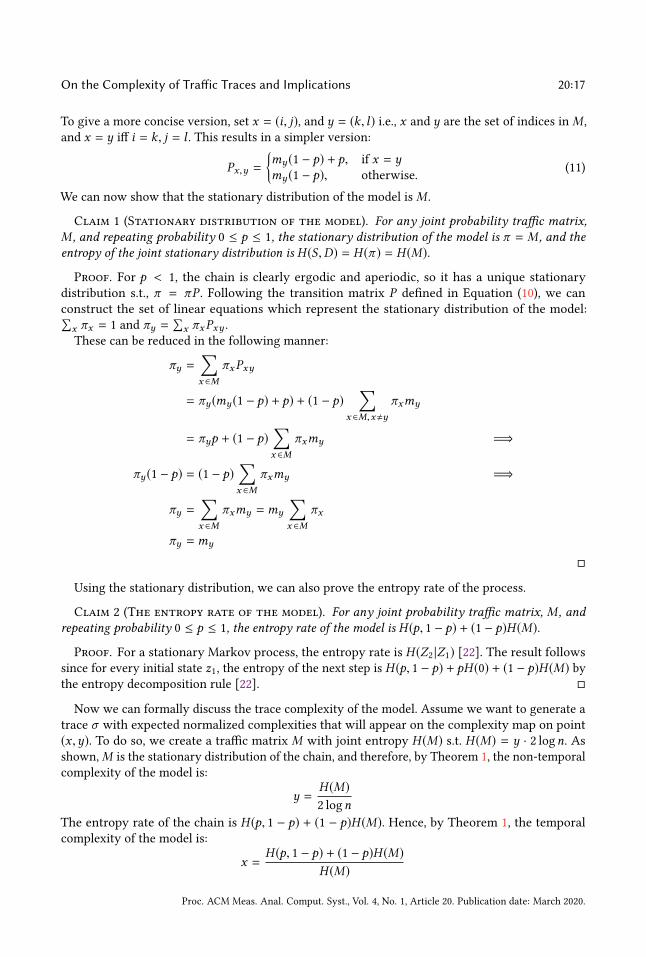
To give a more concise version, set x = (i, j), and y = (k, l) i.e., x and y are the set of indices inM ,
and x = y iff i = k, j = l . This results in a simpler version:
Px,y =
my (1 − p) + p, if x = ymy (1 − p), otherwise.
(11)
We can now show that the stationary distribution of the model isM .
Claim 1 (Stationary distribution of the model). For any joint probability traffic matrix,M , and repeating probability 0 ≤ p ≤ 1, the stationary distribution of the model is π = M , and theentropy of the joint stationary distribution is H (S,D) = H (π ) = H (M).
Proof. For p < 1, the chain is clearly ergodic and aperiodic, so it has a unique stationary
distribution s.t., π = πP . Following the transition matrix P defined in Equation (10), we can
construct the set of linear equations which represent the stationary distribution of the model:∑x πx = 1 and πy =
∑x πxPxy .
These can be reduced in the following manner:
πy =∑x ∈M
πxPxy
= πy (my (1 − p) + p) + (1 − p)∑
x ∈M,x,y
πxmy
= πyp + (1 − p)∑x ∈M
πxmy =⇒
πy (1 − p) = (1 − p)∑x ∈M
πxmy =⇒
πy =∑x ∈M
πxmy =my
∑x ∈M
πx
πy =my
Using the stationary distribution, we can also prove the entropy rate of the process.
Claim 2 (The entropy rate of the model). For any joint probability traffic matrix, M , andrepeating probability 0 ≤ p ≤ 1, the entropy rate of the model is H (p, 1 − p) + (1 − p)H (M).
Proof. For a stationary Markov process, the entropy rate is H (Z2 |Z1) [22]. The result follows
since for every initial state z1, the entropy of the next step is H (p, 1 − p) + pH (0) + (1 − p)H (M) by
the entropy decomposition rule [22].
Now we can formally discuss the trace complexity of the model. Assume we want to generate a
trace σ with expected normalized complexities that will appear on the complexity map on point
(x ,y). To do so, we create a traffic matrix M with joint entropy H (M) s.t. H (M) = y · 2 logn. Asshown,M is the stationary distribution of the chain, and therefore, by Theorem 1, the non-temporal
complexity of the model is:
y =H (M)
2 logn
The entropy rate of the chain is H (p, 1 − p) + (1 − p)H (M). Hence, by Theorem 1, the temporal
complexity of the model is:
x =H (p, 1 − p) + (1 − p)H (M)
H (M)
Proc. ACM Meas. Anal. Comput. Syst., Vol. 4, No. 1, Article 20. Publication date: March 2020.
20:18 Avin et al.
WEB
HPC
ML
Uniform
Skewed
Bursty
Skewed
& Bursty
Original TraceReproduced Trace
0.3 0.4 0.5 0.6 0.7 0.8 0.9 1.0.3
0.4
0.5
0.6
0.7
0.8
0.9
1.
Temporal complexity
Non-temporalcomplexity
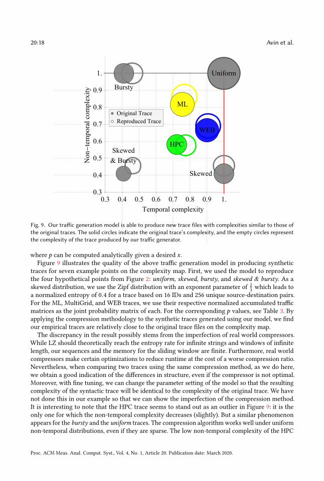
Fig. 9. Our traffic generation model is able to produce new trace files with complexities similar to those ofthe original traces. The solid circles indicate the original trace’s complexity, and the empty circles representthe complexity of the trace produced by our traffic generator.
where p can be computed analytically given a desired x .Figure 9 illustrates the quality of the above traffic generation model in producing synthetic
traces for seven example points on the complexity map. First, we used the model to reproduce
the four hypothetical points from Figure 2: uniform, skewed, bursty, and skewed & bursty. As askewed distribution, we use the Zipf distribution with an exponent parameter of
2
3which leads to
a normalized entropy of 0.4 for a trace based on 16 IDs and 256 unique source-destination pairs.
For the ML, MultiGrid, and WEB traces, we use their respective normalized accumulated traffic
matrices as the joint probability matrix of each. For the corresponding p values, see Table 3. By
applying the compression methodology to the synthetic traces generated using our model, we find
our empirical traces are relatively close to the original trace files on the complexity map.
The discrepancy in the result possibly stems from the imperfection of real world compressors.
While LZ should theoretically reach the entropy rate for infinite strings and windows of infinite
length, our sequences and the memory for the sliding window are finite. Furthermore, real world
compressors make certain optimizations to reduce runtime at the cost of a worse compression ratio.
Nevertheless, when comparing two traces using the same compression method, as we do here,
we obtain a good indication of the differences in structure, even if the compressor is not optimal.
Moreover, with fine tuning, we can change the parameter setting of the model so that the resulting
complexity of the syntactic trace will be identical to the complexity of the original trace. We have
not done this in our example so that we can show the imperfection of the compression method.
It is interesting to note that the HPC trace seems to stand out as an outlier in Figure 9: it is the
only one for which the non-temporal complexity decreases (slightly). But a similar phenomenon
appears for the bursty and the uniform traces. The compression algorithmworks well under uniform
non-temporal distributions, even if they are sparse. The low non-temporal complexity of the HPC
Proc. ACM Meas. Anal. Comput. Syst., Vol. 4, No. 1, Article 20. Publication date: March 2020.
On the Complexity of Traffic Traces and Implications 20:19
trace is a result of the trace being sparse and close to uniform among the participating pairs, as we
observe in Figure 4 (b), and not from its being skewed. We conjecture that in this case, it is “easier"
for the compression algorithm to work well and for the model to capture better the original trace.
5 FROM STRUCTURE TO OPTIMIZATION: A CASE STUDYMetrics to measure the various structures of traffic traces are not only of theoretical interest;
they also have implications for network optimization, in that a a traffic trace with much structure
indicates a high potential for traffic-aware optimizations. In this section, we provide an example
to substantiate our earlier claim that “structure calls for optimization". Specifically, we show that
traces (or applications) with lower complexity can potentially gain from a clever network design.
Because of space constraints, we will skip many technical details and focus on the main intuition.
Our case study is situated in the context of emerging reconfigurable optical networks: networks
whose topologies can be adjusted to meet the demand they serve [9, 10, 21, 34, 39, 41, 42, 64, 80].
We refer to such networks as self-adjusting networks. For our discussion, we consider a recent
self-adjusting network, SASL2 [11, 12]. SASL2 comes with theoretical guarantees which allow us to
tie it to the complexity map and to our generative model. That said, we note that similar claims
could also be made for other network proposals, e.g., SplayNets [64].SASL2 adaptively reconfigures a datacenter topology to minimize routing costs: the path length
between pairwise communicating partners in the trace σ . The algorithm makes a tradeoff between
the benefits and costs of reconfigurations. In particular, because of the different time scales of
packet transmission and reconfiguration, a network can only be changed after having served a
request.
As [12] show, when SASL2 is used, the expected cost of routing a communication request σt froma source st to a destination dt is proportional to the size of the working set of the request, at thetime of the request, denoted asWS(σt ). The working set is a well-known measure of the cost and
efficiency of data structures (e.g., binary search trees and skip lists). Informally it tries to capture
the number of recent “active” elements in the system. More formally, for a sequence of singleton
items x1,x2, . . . xm , the working set of an item x at time t ,WS(xt ) is the number of distinct items
requested since the last request to x prior to time t , including x . For pairwise requests, as in a trace
σ , the definition is a bit more involved, but if we consider σ to be a sequence s1,d1, s2,d2, . . . theworking set is well defined for each xt . A data structure has the working set property if its total
cost to servem items is of the order of
∑mt=1 logWS(xt ). It is known that the working set property
implies the entropy bound, known also as static optimality [31]; i.e.,
∑mt=1 logWS(xt ) = O(mH (X ))
where H (X ) is the empirical entropy of the sequence.
Using the above results we can bound the cost of SASL2 (and similar networks) on a sequence
generated by the generative model described in § 4.2.
Claim 3. For any joint probability traffic matrix, M , and repeating probability 0 ≤ p ≤ 1, theexpected amortized cost of SASL
2 on a sequence generated by the model in §4.2 isO(p + (1 − p)H (Z )),where Z is a random variable over the n possible source or destination IDs and with frequencies impliedbyM .
Proof overview. From [12] we have that SASL2 has the working set property for σ . From the
model, we can conclude that the expected total working set bound will bemp (number of times
repeating the last request) plus the working set cost, but limited to the case of sampling a request
fromM . The latter, in turn, can be shown to be bounded bym(1 − p)H (Z ) using [31].
Consequently, we can state the following:
Proc. ACM Meas. Anal. Comput. Syst., Vol. 4, No. 1, Article 20. Publication date: March 2020.
20:20 Avin et al.
Uniform
Skewed
Bursty
Skewed& Bursty
0.3 0.4 0.5 0.6 0.7 0.8 0.9 1.0.3
0.4
0.5
0.6
0.7
0.8
0.9
1.
Temporal complexity
Non
-temporalcomplexity
e.g., Xpander, Fat-tree, RotorNet
?e.g., Proteus, ProjecToR,
DAN
e.g., SASL2, SplayNet
Fig. 10. A possible partition of the complexity map into regions of dominating designs, for expected pathlength. We hypothesize the locations of Xpaner [48], fat-tree [3], RotorNet [57], ProjecTor [39], DAN [10],SASL2 [12] and SplayNet [64].
Corollary 1. The normalized complexity of a trace σ generated by our model captures theratio of performance improvement in expected route length, to a uniform trace, U(σ ), and to theperformance of a demand-oblivious network design on the same trace.
To elaborate: from Theorem 1 and Claim 2 it follows that the complexity of σ will converge to
H (p,1−p)+(1−p)H (M )
2 logn . But this ratio is proportional to the ratio of the amortized costs (i.e., expected
path length) of σ to the amortized cost of the uniform trace U(σ ) which is:p+(1−p)H (Z )
logn . Note that
a uniform trace can also be generated by the model with p = 0 and a uniform matrixM , leading
to an expected path length of logn. Interestingly, if we consider any static, bounded degree and
demand-oblivious network N , such as Xpander [48] or fat-tree [3], for example, then the average
path length on that network N for any σ will be Ω(logn). This means that the improvement ratio of
executing σ on SASL2 to N (which is static and oblivious) will also be proportional to the complexity
of σ .The above corollary provides a strong indication that complexity captures important aspects of
the trace structure, and in turn, those aspects can be explored to improve performance.
The example raises many interesting questions. Which types of optimizations and algorithms
should we use, given the complexity of a trace? Can certain algorithms work well for initially
unknown complexity? We believe the complexity map could ,help answer these questions, as it
a partition the complexity spectrum into regions indicating the best algorithms. For example, if
we consider the above example of path lengths, we can initially partition the map as shown in
Figure 10 where some (extreme) areas are suspected to be optimal for certain algorithms. But the
majority of the map deals with bursty & skewed traces, and for these traces, it remains an open
question which algorithms are optimal and where. We leave the theoretical and empirical study of
these questions for future work.
Proc. ACM Meas. Anal. Comput. Syst., Vol. 4, No. 1, Article 20. Publication date: March 2020.
On the Complexity of Traffic Traces and Implications 20:21
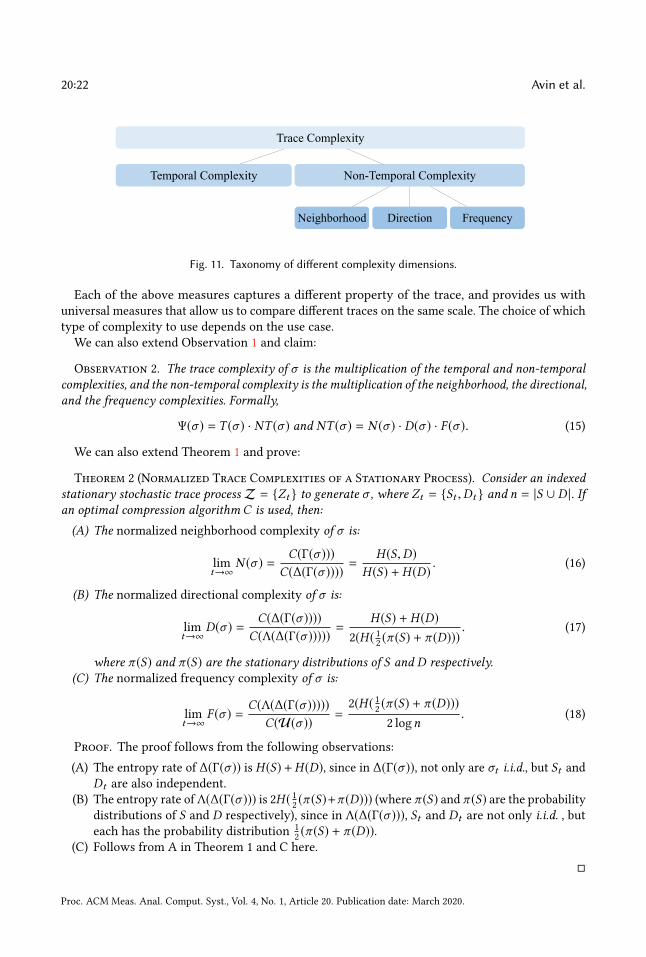
6 REFINED TYPES OF TRACE COMPLEXITIESWhile we focus on temporal and non-temporal complexities in this paper, our method can easily
be refined for other sub-types of complexity. For example, we can subdivide the non-temporal
complexity into three natural categories: neighborhood complexity, directional complexity, andfrequency complexity. See Figure 11. This division adds dimensions to the trace complexity, allowing
us to better understand the structure and to differentiate between traces. As mentioned earlier, two
traces can have the same temporal and non-temporal complexity. The new complexities may help
us distinguish between them.
We begin by introducing two random transformations.
(1) Column transformation, ∆(σ ): This transformation performs a uniformly random shuffle
of the destinations in σ , eliminating any dependency between the sources and the destinations
(without loss of generality, the transformation can be performed on sources only).
(2) Pairs transformation, Λ(σ ): This transformation performs a uniformly random shuffle of
each (source, destination) pair in σ independently eliminating any dependency between
elements’ IDs and their role as sources or destination.
Using the above transformations, we can formally define the new complexities. It is important to
note that the transformations we defined can be applied to a trace σ in different a order, resultingin different complexities. The order we choose follows a natural order that systematically destroys
structure and increases complexity, starting at the original trace σ and ending at the structure-less
U(σ ). First, we use the temporal transformation to remove temporal structure. Next, we use the
column transformation to remove source-destination dependency. Then, we use pairs transformation
to destroy roles (source or destination) of nodes. Last, we use the uniform transformation to reach
U(σ ). An example of this order including ∆(σ ) and Λ(σ ) is shown in Table 1. We define our
complexities according to this order.
Definition 4 (Neighborhood, Directional, and Freqency Trace Complexities Ratios).
Let σ be a traffic trace whose entries are of the form σi = (si ,di ) . We define:(1) The normalized neighborhood trace complexity of σ as:
N (σ ) =C(Γ(σ )))
C(∆(Γ(σ )))). (12)
This captures the complexity that results from the dependency between sources and destinations.For example, a given source could have a strong dependency on which set of destinations itcommunicates with. The column transformation eliminates this dependency.
(2) The normalized directional trace complexity of σ is:
D(σ ) =C(∆(Γ(σ ))))
C(Λ(∆(Γ(σ ))))). (13)
This captures the complexity resulting from the role of elements as sources or destinations. Forexample the sets of sources and destinations can be of a different size and, in an extreme exampledisjoint. The pair transformation eliminates this structure.
(3) The normalized frequency trace complexity of σ is:
F (σ ) =C(Λ(∆(Γ(σ )))))
C(U(σ )). (14)
This captures the complexity that results from the frequency distribution of elements in thesequence. For example, several elements (sources or destinations) can be much more popular thanothers. The uniform transformation eliminates this property and ensures a uniform distributionof elements.
Proc. ACM Meas. Anal. Comput. Syst., Vol. 4, No. 1, Article 20. Publication date: March 2020.
20:22 Avin et al.
Neighborhood
Trace Complexity
Non-Temporal Complexity
Direction Frequency
Temporal Complexity
Fig. 11. Taxonomy of different complexity dimensions.
Each of the above measures captures a different property of the trace, and provides us with
universal measures that allow us to compare different traces on the same scale. The choice of which
type of complexity to use depends on the use case.
We can also extend Observation 1 and claim:
Observation 2. The trace complexity of σ is the multiplication of the temporal and non-temporalcomplexities, and the non-temporal complexity is the multiplication of the neighborhood, the directional,and the frequency complexities. Formally,
Ψ(σ ) = T (σ ) · NT (σ ) and NT (σ ) = N (σ ) · D(σ ) · F (σ ). (15)
We can also extend Theorem 1 and prove:
Theorem 2 (Normalized Trace Complexities of a Stationary Process). Consider an indexedstationary stochastic trace processZ = Zt to generate σ , where Zt = St ,Dt and n = |S ∪ D |. Ifan optimal compression algorithm C is used, then:
(A) The normalized neighborhood complexity of σ is:
lim
t→∞N (σ ) =
C(Γ(σ )))
C(∆(Γ(σ ))))=
H (S,D)
H (S) + H (D). (16)
(B) The normalized directional complexity of σ is:
lim
t→∞D(σ ) =
C(∆(Γ(σ ))))
C(Λ(∆(Γ(σ )))))=
H (S) + H (D)
2(H ( 12(π (S) + π (D)))
. (17)
where π (S) and π (S) are the stationary distributions of S and D respectively.(C) The normalized frequency complexity of σ is:
lim
t→∞F (σ ) =
C(Λ(∆(Γ(σ )))))
C(U(σ ))=
2(H ( 12(π (S) + π (D)))
2 logn. (18)
Proof. The proof follows from the following observations:
(A) The entropy rate of ∆(Γ(σ )) is H (S)+H (D), since in ∆(Γ(σ )), not only are σt i.i.d., but St andDt are also independent.
(B) The entropy rate ofΛ(∆(Γ(σ ))) is 2H ( 12(π (S)+π (D))) (where π (S) and π (S) are the probability
distributions of S and D respectively), since in Λ(∆(Γ(σ ))), St and Dt are not only i.i.d. , buteach has the probability distribution
1
2(π (S) + π (D)).
(C) Follows from A in Theorem 1 and C here.
Proc. ACM Meas. Anal. Comput. Syst., Vol. 4, No. 1, Article 20. Publication date: March 2020.
On the Complexity of Traffic Traces and Implications 20:23
7 RELATEDWORKThe study of traffic patterns and the design of models is a popular topic, with high relevance in the
networking literature, as it has important implications, e.g., on network planning and provisioning.
For example, it has been shown that the best design choice for a datacenter network architecture
(in terms of cost/benefit tradeoff) depends on the communication pattern between end hosts [59],
but lacking concrete data, researchers often resort to designing networks for the worst case, i.e., an
all-to-all traffic matrix [3] which can be overkill when demand exhibits significant locality [27, 39].
A well-known example in the literature where measurement studies spurred much research
into traffic modeling dates back to the 1990s, when researchers found that, in strong contrast to
traditional models relying on Poisson assumptions [50], traffic in local-area and wide-area networks
is “self-similar” in that it exhibits variability on a wide range of scales [25, 50, 53]. Motivated by
these results, researchers developed a number of models [58], e.g., related to the heavy-tailed
distribution of transferred file sizes, properties of the transport/network layer in the protocol stack,
ON/OFF traffic models such as [68], etc. Much modeling research also went into generating diskI/O traces often described by mixing sequential and random accesses [66],
More systematically, works on network traffic modeling includes temporal statistical models
such as AutoRegressive Integrated Moving Average (ARIMA) [38], Multifractal Wavelets [61], and
b-model [74],which are used to describe temporal burstiness. Spatial statistics models for “smooth
traffic” often rely on (multivariate) Gaussian distributions [24] and marked point processes [23] areused to model events in time and space.
It is interesting to put our work into the context of this previous work. Like others before us we
are studying the temporal structure of traces. But there are several key differences. First, we focus
on the source-destination structure/complexity of the traces, not on the accumulative traffic load
as in previous models. This leads to an additional dimension in the trace and to new observations.
Second, we use the entropy and the entropy rate as the main metrics to quantify the structure.
Although not explicitly mentioned, some of the above models can be characterized by their entropy.
For example, the self-similar traffic models, e.g., ARIMA, are known to be captured well by their
entropy rate [22]. In particular the only source of uncertainty stems from the noise, and the entropy
depends on the variance of the Gaussian process. In future work, we plan to add load or packet
(flow) size information to the trace; it will also be useful to incorporate some of the above methods,
including spectral analysis.
Physical models aim to simulate user behavior; a classic example is the ON/OFF model [15] in
web traffic generators where the user’s thinking time follows a heavy-tailed distribution. Some
interesting work in this area proposes to model multiple dimensions simultaneously, e.g., the
spatio-temporal behavior [73].
Motivated by the high potential utility of a traffic matrix for network capacity planning and
management, many researchers have studied how to measure and estimate the traffic matrix [56].
A well-known and simple model is the gravity model- [60, 62] which assumes the amount of traffic
between two nodes is proportional (only) to the product of the total traffic entering or leaving the
two nodes. In their interesting work, Zhang et al. [79] show that link load measurements can be
used to quickly and accurately infer traffic matrices in IP networks, by enhancing the gravity model
(which is guaranteed to be consistent with measured link loads at the network edge but not theinterior links) with tomographic methods [20, 71]. Tomographic methods have also been applied to
the detection of network-level anomalies, e.g., based on Fourier transform and Principal Component
Analysis models [78]. However, most of these models revolve around (static) “snapshots” of the
communication pattern and do not provide many insights into the evolution over time. We are
more interested in the granularity of traffic traces than entire traffic matrices.
Proc. ACM Meas. Anal. Comput. Syst., Vol. 4, No. 1, Article 20. Publication date: March 2020.
20:24 Avin et al.
In this paper, we are particularly interested in the traffic matrices from in datacenters andtheir evolution over time. The presence of such structures and models can give important insights
into the usefulness of recent reconfigurable networking technologies, e.g., malleable datacenter
topologies [12, 13, 21, 34, 36, 39, 41–43, 54, 67, 80] (cf. the recent survey [37]). Underlying all these
technologies is the hope of being able to leverage “structure” in demand patterns and, by adapting
the network over time accordingly, realizing cheaper and more efficient datacenter networks. In
this context, Avin et al. recently established a connection between demand-aware network designs
and information theory, showing that achievable routing performance relies on the (conditional)
entropy of the demand [10, 14, 64? ].Unfortunately, few empirical studies report on traffic patterns in datacenters, and the data
available to the research community is severely limited. Many studies rely on simulations [4] or
testbeds [32]. The exceptions are often limited to workload traces from a single, large datacenter [16,
46], dominated by Web search related traffic. Existing empirical studies, however, all confirm that
traffic patterns in datacenters have “low entropy”: they feature much (spatial and temporal) locality,i.e., are sparse and skewed [5, 39, 44, 63].
More specifically, empirical studies of datacenter networks show that much traffic is rack-
local [16, 27], demand is frequently concentrated and bursty [16–18, 27], packets have bimodal
sizes, traffic features ON/OFF behavior [16], and there is a small number of large flows [5]. Some
of these properties were recently revisited a large empirical study in Facebook’s datacenters [63]:
the authors find that their datacenters provide a richer picture. Their traffic is neither rack-local
nor all-to-all, demand is wide-spread, uniform, and stable, with rapidly changing, internally bursty
heavy hitters, packets are typically small (outside of Hadoop), arrivals are continuous, and there
are many concurrent flows.
Finally, we are not the first to use adaptive data compression for complexity analysis, and similar
methodologies have been proposed elsewhere, e.g., for email [19] or comment [47] spam filtering, or
to estimate neural discharges [8]. Entropy rates [49] have also been investigated intensively in the
literature, e.g., for feature selection in machine learning [30]. However, to the best of our knowledge,
such approaches have not been considered in the context of network traffic characterization.
8 CONCLUSION AND DISCUSSIONWhile many research efforts focus on leveraging the structure of packet traces to design more
efficient datacenter networks, the community currently lacks a formal understanding of the amount
and types of structures available in traffic traces. This paper takes the first steps towards developing
a formal framework and metrics to systematically quantify temporal and non-temporal structures
in datacenter workloads.
Indeed, practitioners are often unaware of their application traffic behavior. The sheer volume of
traffic, as well as the amount of storage required to store the trace files, hinders datacenter providers
to keep detailed profiles of their traffic. Our approach can enable datacenter providers to use trace
complexity as a tool to maintain a profile of various applications and plan for datacenter resources
accordingly. For instance a typical datacenter switch has 128 ports each port with 100 Gbps. Such a
switch will generate 12.8 Tbps data. Collecting this traffic for even 5 minutes puts much pressure
on the CPU and can overload the storage servers (5 min of 12.8 Tbps traffic yields 3.8 Pb). As a
result, traffic monitoring is almost always off and providers are unaware of the trace complexity of
applications.
Clearly, low-dimensional representations of the trace structure such as a 2-dimensional complex-
ity map, inevitably comes with a loss of information, and many different traces end up on the same
location in the space. However, these dimensions can be sufficient to capture the essential part
of the trace. For example, the non-temporal complexity, i.e., the conditional entropy, of a packet
Proc. ACM Meas. Anal. Comput. Syst., Vol. 4, No. 1, Article 20. Publication date: March 2020.
On the Complexity of Traffic Traces and Implications 20:25
trace, is sufficient to describe accurately the achievable route lengths in a static constant-degree
demand-aware networks [10]. It is hence the “right metric” for this application and other aspects
of the trace are irrelevant.
That said, a nice feature of our approach is that it can be seen as a framework: we can account
for additional dimensions, such as packet arrival times or packet sizes, by systematically using
randomization to eliminate structure along these dimensions as well. And indeed, identifying and
incorporating such additional dimensions constitutes an interesting avenue for future research. At
the same time, as discussed above, adding more dimensions indiscriminately should be avoided:
the challenge when applying our framework is not to maximize the number of dimensions but to
find a small number of “most valuable dimensions”, ie., the dimensions which capture the essential
part of the traces for a specific application.
For example, recall again the demand-aware network application discussed above: all traces
featuring the same non-temporal complexity (i.e., entropy), no matter how different they are, result
in exactly the same expected route lengths (up to constant factors and under sparse demands [10])
in bounded-degree, demand-aware networks. Hence this simple metric is sufficient to accurately
characterize what can and cannot be achieved in demand-aware network topologies. Our approach
of iteratively randomizing and compressing traces raises the question of the optimal order in which
structure is removed. More generally, it will be interesting to explore to what extent our proposed
traffic generation model can be used to benchmark future scheduling, congestion control, and
reconfigurable datacenter proposals. We also note that while the focus in our paper was on the
complexity of traffic traces arising communication networks, our approach is more general and
may find interesting applications in other dynamic contexts as well.
To facilitate future research and ensure reproducibility of our results, we made our traces and
model publicly available at trace-collection.net.
ACKNOWLEDGMENTSWe would like to thank our shepherd Sara Alouf and the reviewers for their time and suggestions
on how to improve the paper. We are also grateful to Walter Willinger for his insightful feedback
and to Asaf Cohen for interesting discussions about the topic. This project has received funding
from the European Research Council (ERC) under the European Union’s Horizon 2020 research
and innovation programme (grant agreement No. 864228, AdjustNet: Self-Adjusting Networks).
[3] Mohammad Al-Fares, Alexander Loukissas, and Amin Vahdat. 2008. A Scalable, Commodity Data Center Network
Architecture. Proc. SIGCOMM Computer Communication Review (CCR) 38, 4 (Aug. 2008), 63–74. https://doi.org/10.
1145/1402946.1402967
[4] Alaa R Alameldeen, Milo MK Martin, Carl J Mauer, Kevin E Moore, Min Xu, Mark D Hill, David A Wood, and Daniel J
Sorin. 2003. Simulating a $2 M Commercial Server on a $2 K PC. IEEE Computer 36, 2 (2003), 50–57.[5] Mohammad Alizadeh, Albert Greenberg, David A Maltz, Jitendra Padhye, Parveen Patel, Balaji Prabhakar, Sudipta
Sengupta, and Murari Sridharan. 2010. Data Center TCP (DCTCP). In Proc. ACM SIGCOMM Computer CommunicationReview (CCR), Vol. 40. 63–74.
[6] Mohammad Alizadeh, Shuang Yang, Milad Sharif, Sachin Katti, Nick McKeown, Balaji Prabhakar, and Scott Shenker.
2013. pFabric: Minimal near-optimal datacenter transport. In ACM SIGCOMM Computer Communication Review, Vol. 43.ACM, 435–446.
[7] Mohammad Alizadeh, Shuang Yang, Milad Sharif, Sachin Katti, Nick McKeown, Balaji Prabhakar, and Scott Shenker.
2013. pFabric: Minimal Near-optimal Datacenter Transport. In Proceedings of the ACM SIGCOMM 2013 Conference onSIGCOMM (SIGCOMM ’13). ACM, New York, NY, USA, 435–446. https://doi.org/10.1145/2486001.2486031
[8] José M Amigó, Janusz Szczepański, Elek Wajnryb, and Maria V Sanchez-Vives. 2004. Estimating the Entropy Rate of
[9] Chen Avin, Alexandr Hercules, Andreas Loukas, and Stefan Schmid. 2018. rDAN: Toward Robust Demand-Aware
Network Designs. In Information Processing Letters (IPL), Vol. 133. 5–9.[10] Chen Avin, KaushikMondal, and Stefan Schmid. 2017. Demand-Aware Network Designs of Bounded Degree. Distributed
Computing (2017), 1–15.
[] Chen Avin, Kaushik Mondal, and Stefan Schmid. 2019. Demand-Aware Network Design with Minimal Congestion and
Route Lengths. In IEEE INFOCOM 2019-IEEE Conference on Computer Communications. IEEE, 1351–1359.[11] Chen Avin, Iosif Salem, and Stefan Schmid. 2019. Brief Announcement: On Self-Adjusting Skip List Networks. In Proc.
33rd International Symposium on Distributed Computing (DISC). Dagstuhl, Germany.
[12] Chen Avin, Iosif Salem, and Stefan Schmid. 2020. Working Set Theorems for Routing in Self-Adjusting Skip List
Networks. In Proc. IEEE INFOCOM.
[13] Chen Avin and Stefan Schmid. 2019. ReNets: Toward Statically Optimal Self-Adjusting Networks. arXiv preprintarXiv:1904.03263 (2019).
[14] Chen Avin and Stefan Schmid. 2019. Toward demand-aware networking: A theory for self-adjusting networks. ACMSIGCOMM Computer Communication Review 48, 5 (2019), 31–40.
[15] Paul Barford and Mark Crovella. 1998. Generating Representative WebWorkloads for Network and Server Performance
[16] Theophilus Benson, Aditya Akella, and David A Maltz. 2010. Network Traffic Characteristics of Data Centers in the
Wild. In Proc. ACM SIGCOMM Conference on Internet Measurement (IMC). ACM, 267–280.
[17] Theophilus Benson, Ashok Anand, Aditya Akella, and Ming Zhang. 2009. Understanding Data Center Traffic Charac-
teristics. In Proc. 1st ACM Workshop on Research on Enterprise Networking (WREN). ACM, 65–72.
[18] Theophilus Benson, Ashok Anand, Aditya Akella, and Ming Zhang. 2011. MicroTE: Fine Grained Traffic Engineering
for Data Centers. In Proc. 7th Conference on emerging Networking EXperiments and Technologies (CoNEXT). ACM, 8.
[19] Andrej Bratko, Gordon V Cormack, Bogdan Filipič, Thomas R Lynam, and Blaž Zupan. 2006. Spam Filtering Using
Statistical Data Compression Models. Journal of machine learning research 7, Dec (2006), 2673–2698.
[20] Jin Cao, Drew Davis, Scott Vander Wiel, and Bin Yu. 2000. Time-Varying Network Tomography: Router Link Data.
Journal of the American statistical association 95, 452 (2000), 1063–1075.
[21] Kai Chen, Ankit Singla, Atul Singh, Kishore Ramachandran, Lei Xu, Yueping Zhang, Xitao Wen, and Yan Chen. 2014.
OSA: An Optical Switching Architecture for Data Center Networks With Unprecedented Flexibility. IEEE/ACMTransactions on Networking (TON) 22, 2 (2014), 498–511.
[22] Thomas M Cover and Joy A Thomas. 2012. Elements of information theory. John Wiley & Sons.
[23] David Roxbee Cox and Valerie Isham. 1980. Point Processes. Vol. 12. CRC Press.
[24] Noel Cressie. 1992. Statistics for Spatial Data. Terra Nova 4, 5 (1992), 613–617.[25] Mark E Crovella and Azer Bestavros. 1997. Self-Similarity in World Wide Web Traffic: Evidence and Possible Causes.
IEEE/ACM Transactions on networking 5, 6 (1997), 835–846.
[27] Christina Delimitrou, Sriram Sankar, Aman Kansal, and Christos Kozyrakis. 2012. ECHO: Recreating Network
Traffic Maps for Datacenters with Tens of Thousands of Servers. In Proc. IEEE International Symposium on WorkloadCharacterization (IISWC). IEEE, 14–24.
[28] Peter Deutsch. 1996. DEFLATE compressed data format specification version 1.3. Technical Report.[29] US DOE. 2016. Characterization of the DOE Mini-apps. https://portal.nersc.gov/project/CAL/doe-miniapps.htm.
[30] Garry A Einicke, Haider A Sabti, David V Thiel, and Marta Fernandez. 2017. Maximum-Entropy-Rate Selection of
Features for Classifying Changes in Knee and Ankle Dynamics During Running. IEEE Journal of Biomedical and HealthInformatics (2017).
[31] Amr Elmasry, Arash Farzan, and John Iacono. 2013. On the Hierarchy of Distribution-Sensitive Properties for Data
Structures. Acta informatica 50, 4 (2013), 289–295.[32] Deniz Ersoz, Mazin S Yousif, and Chita R Das. 2007. Characterizing Network Traffic in a Cluster-Based, Multi-Tier
Data Center. In Proc. IEEE 27th International Conference on Distributed Computing Systems (ICDCS). IEEE, 59.[33] E Estevez-Rams, R Lora Serrano, B Aragon Fernandez, and I Brito Reyes. 2013. On the Non-Randomness of Maximum
Lempel Ziv Complexity Sequences of Finite Size. Chaos: An Interdisciplinary Journal of Nonlinear Science 23, 2 (2013),023118.
Yeshaiahu Fainman, George Papen, and Amin Vahdat. 2010. Helios: a Hybrid Electrical/Optical Switch Architecture
for Modular Data Centers. Proc. ACM SIGCOMM Computer Communication Review (CCR) 40, 4 (2010), 339–350.[35] Meir Feder, Neri Merhav, and Michael Gutman. 1992. Universal Prediction of Individual Sequences. IEEE Transactions
on Information Theory 38, 4 (1992), 1258–1270.
Proc. ACM Meas. Anal. Comput. Syst., Vol. 4, No. 1, Article 20. Publication date: March 2020.
Alexandre Blanche, Houman Rastegarfar, Madeleine Glick, and Daniel Kilper. 2016. ProjecToR: Agile Reconfigurable
Data Center Interconnect. In Proc. ACM SIGCOMM. ACM, New York, NY, USA, 216–229. https://doi.org/10.1145/
2934872.2934911
[40] Geoffrey Gunow, John Tramm, Benoit Forget, Kord Smith, and Tim He. 2015. SimpleMOC – A Performance Ab-
straction for 3D MOC. In ANS & M&C 2015 - Joint International Conference on Mathematics and Computation (M&C),Supercomputing in Nuclear Applications (SNA) and the Monte Carlo (MC) Method.
[41] Daniel Halperin, Srikanth Kandula, Jitendra Padhye, Paramvir Bahl, and David Wetherall. 2011. Augmenting Data
Center Networks with Multi-Gigabit Wireless Links. ACM SIGCOMM Computer Communication Review 41, 4, 38–49.
[42] Navid Hamedazimi, Zafar Qazi, Himanshu Gupta, Vyas Sekar, Samir R Das, Jon P Longtin, Himanshu Shah, and Ashish
Tanwer. 2014. Firefly: A Reconfigurable Wireless Data Center Fabric Using Free-Space Optics. In Proc. ACM SIGCOMMComputer Communication Review (CCR), Vol. 44. 319–330.
[43] Su Jia, Xin Jin, Golnaz Ghasemiesfeh, Jiaxin Ding, and Jie Gao. 2017. Competitive Analysis for Online Scheduling in
Software-Defined Optical WAN. In IEEE INFOCOM 2017-IEEE Conference on Computer Communications. IEEE, 1–9.[44] Glenn Judd. 2015. Attaining the Promise and Avoiding the Pitfalls of TCP in the Datacenter.. In Proc. USENIX Symposium
on Networked Systems Design and Implementation (NSDI). 145–157.[45] A Kaitchenko. 2004. Algorithms for Estimating Information Distance with Application to Bioinformatics and Linguistics.
In Canadian Conference on Electrical and Computer Engineering 2004 (IEEE Cat. No. 04CH37513), Vol. 4. IEEE, 2255–2258.[46] Srikanth Kandula, Sudipta Sengupta, Albert Greenberg, Parveen Patel, and Ronnie Chaiken. 2009. The Nature of Data
Center Traffic: Measurements & Analysis. In Proc. 9th ACM Internet Measurement Conference (IMC). 202–208.[47] Alex Kantchelian, Justin Ma, Ling Huang, Sadia Afroz, Anthony Joseph, and JD Tygar. 2012. Robust Detection of
Comment Spam Using Entropy Rate. In Proc. 5th ACM Workshop on Security and Artificial Intelligence. ACM, 59–70.
[48] Simon Kassing, Asaf Valadarsky, Gal Shahaf, Michael Schapira, and Ankit Singla. 2017. Beyond Fat-Trees Without
Antennae, Mirrors, and Disco-Balls. In Proc. ACM SIGCOMM. 281–294.
[49] Matthew B Kennel, Jonathon Shlens, Henry DI Abarbanel, and EJ Chichilnisky. 2005. Estimating Entropy Rates with
[50] Will E Leland, Murad S Taqqu, Walter Willinger, and Daniel V Wilson. 1994. On the Self-Similar Nature of Ethernet
Traffic (extended version). IEEE/ACM Transactions on Networking (ToN) 2, 1 (1994), 1–15.[51] Abraham Lempel and Jacob Ziv. 1976. On the Complexity of Finite Sequences. IEEE Transactions on information theory
22, 1 (1976), 75–81.
[52] Ming Li and Paul Vitányi. 2008. An Introduction to Kolmogorov Complexity and its Applications. Vol. 3. Springer.[53] Nikolai Likhanov, Boris Tsybakov, and Nicolas D Georganas. 1995. Analysis of an ATM Buffer with Self-Similar
("Fractal") Input Traffic. In Proc. IEEE INFOCOM, Vol. 3. IEEE, 985–992.
[54] He Liu, Feng Lu, Alex Forencich, Rishi Kapoor, Malveeka Tewari, Geoffrey M Voelker, George Papen, Alex C Snoeren,
and George Porter. 2014. Circuit Switching Under the Radar with REACToR.. In Proc. USENIX Symposium on NetworkedSystems Design and Implementation (NSDI), Vol. 14. 1–15.
[55] Hongzi Mao, Ravi Netravali, and Mohammad Alizadeh. 2017. Neural Adaptive Video Streaming with Pensieve. In
Proceedings of the Conference of the ACM Special Interest Group on Data Communication (SIGCOMM ’17). ACM, New
York, NY, USA, 197–210. https://doi.org/10.1145/3098822.3098843
[56] Alberto Medina, Nina Taft, Kave Salamatian, Supratik Bhattacharyya, and Christophe Diot. 2002. Traffic Matrix
Estimation: Existing Techniques and New Directions. In ACM SIGCOMM Computer Communication Review, Vol. 32.ACM, 161–174.
[57] William M Mellette, Rob McGuinness, Arjun Roy, Alex Forencich, George Papen, Alex C Snoeren, and George Porter.
2017. RotorNet: A Scalable, Low-complexity, Optical Datacenter Network. In Proc. ACM SIGCOMM. 267–280.
[58] Kihong Park, Gitae Kim, and Mark Crovella. 1996. On the Relationship Between File Sizes, Transport Protocols, and
Self-Similar Network Traffic. In Network Protocols, 1996. Proceedings., 1996 International Conference on. IEEE, 171–180.[59] Lucian Popa, Sylvia Ratnasamy, Gianluca Iannaccone, Arvind Krishnamurthy, and Ion Stoica. 2010. A Cost Comparison
of Datacenter Network Architectures. In Proc. ACM CoNEXT. ACM, 16.
[60] Pentti Pöyhönen. 1963. A Tentative Model for the Volume of Trade Between Countries. Weltwirtschaftliches Archiv(1963), 93–100.
Proc. ACM Meas. Anal. Comput. Syst., Vol. 4, No. 1, Article 20. Publication date: March 2020.
[61] Rudolf H Riedi, Matthew S Crouse, Vinay J Ribeiro, and Richard G Baraniuk. 1999. A Multifractal Wavelet Model with
Application to Network Traffic. IEEE Transactions on Information Theory 45, 3 (1999), 992–1018.
[62] Matthew Roughan, Albert Greenberg, Charles Kalmanek, Michael Rumsewicz, Jennifer Yates, and Yin Zhang. 2003.
Experience in Measuring Internet Backbone Traffic Variability: Models Metrics, Measurements and Meaning. In
Teletraffic Science and Engineering. Vol. 5. Elsevier, 379–388.[63] Arjun Roy, Hongyi Zeng, Jasmeet Bagga, George Porter, and Alex C. Snoeren. 2015. Inside the Social Network’s
(Datacenter) Network. In Proceedings of the 2015 ACM Conference on Special Interest Group on Data Communication(Proc. ACM SIGCOMM). ACM, New York, NY, USA, 123–137. https://doi.org/10.1145/2785956.2787472
[64] Stefan Schmid, Chen Avin, Christian Scheideler, Michael Borokhovich, Bernhard Haeupler, and Zvi Lotker. 2015.
SplayNet: Towards Locally Self-Adjusting Networks. IEEE/ACM Transactions on Networking 24, 3 (2015), 1421–1433.
[65] Claude Elwood Shannon. 1948. A Mathematical Theory of Communication. Bell system technical journal 27, 3 (1948),379–423.
[66] Elizabeth Shriver, Arif Merchant, and John Wilkes. 1998. An Analytic Behavior Model for Disk Drives with Readahead
Caches and Request Reordering. In ACM SIGMETRICS Performance Evaluation Review, Vol. 26. ACM, 182–191.
[67] Ankit Singla, Atul Singh, Kishore Ramachandran, Lei Xu, and Yueping Zhang. 2010. Proteus: a Topology Malleable
Data Center Network. In Proc. ACM Workshop on Hot Topics in Networks (HotNets). ACM, 8.
[68] Murad S Taqqu, Vadim Teverovsky, and Walter Willinger. 1995. Estimators for Long-Range Dependence: an Empirical
Study. Fractals 3, 04 (1995), 785–798.[69] Kun Tu, Bruno Ribeiro, Ananthram Swami, and Don Towsley. 2018. Tracking Groups in Mobile Network Traces. In
Proceedings of the 2018 Workshop on Network Meets AI & ML (NetAI’18). ACM, New York, NY, USA, 35–40. https:
//doi.org/10.1145/3229543.3229552
[70] Asaf Valadarsky, Michael Schapira, Dafna Shahaf, and Aviv Tamar. 2017. Learning to Route. In Proceedings ofthe 16th ACM Workshop on Hot Topics in Networks (HotNets-XVI). ACM, New York, NY, USA, 185–191. https:
//doi.org/10.1145/3152434.3152441
[71] Yehuda Vardi. 1996. Network Tomography: Estimating Source-Destination Traffic Intensities from Link Data. Journalof the American statistical association 91, 433 (1996), 365–377.
[72] Brian Vegetabile, Jenny Molet, Tallie Z Baram, and Hal Stern. 2017. Estimating the Entropy Rate of Finite Markov
Chains with Application to Behavior Studies. arXiv preprint arXiv:1711.03962 (2017).[73] Mengzhi Wang, Anastassia Ailamaki, and Christos Faloutsos. 2002. Capturing the Spatio-Temporal Behavior of Real
[74] Mengzhi Wang, Tara Madhyastha, Ngai Hang Chan, Spiros Papadimitriou, and Christos Faloutsos. 2002. Data
Mining Meets Performance Evaluation: Fast Algorithms For Modeling Bursty Traffic. In Proceedings 18th InternationalConference on Data Engineering. IEEE, 507–516.
[75] Aaron D Wyner and Jacob Ziv. 1994. The Sliding-Window Lempel-Ziv Algorithm is Asymptotically Optimal. Proc.IEEE 82, 6 (1994), 872–877.
[76] Shihan Xiao, Dongdong He, and Zhibo Gong. 2018. Deep-Q: Traffic-driven QoS Inference Using Deep Generative
Network. In Proceedings of the 2018 Workshop on Network Meets AI & ML (NetAI’18). ACM, New York, NY, USA, 67–73.
https://doi.org/10.1145/3229543.3229549
[77] Qiao Zhang, Vincent Liu, Hongyi Zeng, and Arvind Krishnamurthy. 2017. High-resolution Measurement of Data
Center Microbursts. In Proceedings of the 2017 Internet Measurement Conference (IMC ’17). ACM, New York, NY, USA,
78–85. https://doi.org/10.1145/3131365.3131375
[78] Yin Zhang, Zihui Ge, Albert Greenberg, and Matthew Roughan. 2005. Network Anomography. In Proc. 5th ACMSIGCOMM Conference on Internet Measurement (IMC). 30–30.
[79] Yin Zhang, Matthew Roughan, Nick Duffield, and Albert Greenberg. 2003. Fast Accurate Computation of Large-scale
IP Traffic Matrices from Link Loads. In Proc ACM SIGMETRICS International Conference on Measurement and Modelingof Computer Systems. ACM, New York, NY, USA, 206–217. https://doi.org/10.1145/781027.781053
[80] Xia Zhou, Zengbin Zhang, Yibo Zhu, Yubo Li, Saipriya Kumar, Amin Vahdat, Ben Y Zhao, and Haitao Zheng. 2012.
Mirror Mirror on the Ceiling: Flexible Wireless Links for Data Centers. Proc. ACM SIGCOMM Computer CommunicationReview (CCR) 42, 4 (2012), 443–454.
[81] Jacob Ziv and Abraham Lempel. 1977. A Universal Algorithm for Sequential Data Compression. IEEE Transactions oninformation theory 23, 3 (1977), 337–343.
[82] Jacob Ziv and Abraham Lempel. 1978. Compression of Individual Sequences Via Variable-Rate Coding. IEEE Transactionson Information Theory 24, 5 (1978), 530–536.
[83] Shihong Zou, Xitao Wen, Kai Chen, Shan Huang, Yan Chen, Yongqiang Liu, Yong Xia, and Chengchen Hu. 2014.
VirtualKnotter: Online Virtual Machine Shuffling for Congestion Resolving in Virtualized Datacenter. ComputerNetworks 67 (2014), 141–153.
Proc. ACM Meas. Anal. Comput. Syst., Vol. 4, No. 1, Article 20. Publication date: March 2020.