ON THE COMPUTATION OF A TRUNCATED SVD OF

A LARGE LINEAR DISCRETE ILL-POSED PROBLEM

ENYINDA ONUNWOR∗ AND LOTHAR REICHEL†

Dedicated to Ken Hayami on the occasion of his 60th birthday.

Abstract. The singular value decomposition is commonly used to solve linear discrete ill-posedproblems of small to moderate size. This decomposition not only can be applied to determine anapproximate solution, but also provides insight into properties of the problem. However, large-scaleproblems generally are not solved with the aid of the singular value decomposition, because its compu-tation is considered too expensive. This paper shows that a truncated singular value decomposition,made up of a few of the largest singular values and associated right and left singular vectors, of thematrix of a large-scale linear discrete ill-posed problem can be computed quite inexpensively by animplicitly restarted Golub–Kahan bidiagonalization method. Similarly, for large symmetric discreteill-posed problems a truncated eigendecomposition can be computed inexpensively by an implicitlyrestarted symmetric Lanczos method.

1. Introduction. We are concerned with the solution of large least-squaresproblems

minx∈Rn

‖Ax− b‖, A ∈ Rm×n, b ∈ R

m, m ≥ n, (1.1)

with a matrix A, whose singular values gradually decay to zero without a significantgap. In particular, A is very ill-conditioned and may be rank-deficient. Least-squaresproblems with a matrix of this kind are commonly referred to as linear discrete ill-posed problems. Such least-squares problems arise, for instance, from the discretiza-tion of linear ill-posed problems, such as Fredholm integral equations of the first kindwith a continuous kernel. The vector b in linear discrete ill-posed problems that arisein applications in science and engineering typically represents data that are contam-inated by a measurement error e ∈ R

m. Sometimes we will refer to the vector e as“noise.” Thus,

b = btrue + e, (1.2)

where btrue ∈ Rm represents the unknown error-free vector associated with the avail-

able vector b. To simplify the notation, we will assume thatm ≥ n, but this restrictioncan be removed. Throughout this paper ‖ · ‖ denotes the Euclidean vector norm orthe spectral matrix norm.

Let A† denote the Moore–Penrose pseudoinverse of A. We would like to determinean approximation of xtrue = A†btrue by computing an approximate solution of (1.1).Note that the vector x = A†b = xtrue + A†e typically is a useless approximation ofxtrue because, due to the ill-conditioning of A, generally, ‖A†e‖ ≫ ‖xtrue‖.Linear discrete ill-posed problems with a small matrix A are commonly solved withthe aid of the singular value decomposition (SVD) of the matrix; see, e.g., [23, 31]

∗Department of Mathematical Sciences, Kent State University, Kent, OH 44242, USA, and De-partment of Mathematics, Stark State College, 6200 Frank Ave. NW, North Canton, OH 44720,USA. E-mail: eonunwor@starkstate.edu.

†Department of Mathematical Sciences, Kent State University, Kent, OH 44242, USA. E-mail:reichel@math.kent.edu.

1

and references therein. However, it is expensive to compute the SVD of a generallarge matrix; the computation of the SVD of an n × n matrix requires about 22n3

arithmetic floating-point operations (flops); see, e.g., [21, Chapter 8] for details aswell as for flop counts for the situation when m > n. In particular, the SVD of alarge general m×n matrix is very expensive to compute. Therefore, large-scale lineardiscrete ill-posed problems (1.1) are sometimes solved by hybrid methods that firstreduce a large least-squares problem to a least-squares problem of small size by aKrylov subspace method, and then solve the latter by using the SVD of the reducedmatrix so obtained; see, e.g., [19, 32] for discussions.

The need to compute the largest or a few of the largest singular values and, generally,also the associated right and left singular vectors of a large matrix of a linear dis-crete ill-posed problems arises in a variety of applications including the approximateminimization of the generalized cross validation function for determining the amountof regularization [17], the solution of large-scale discrete ill-posed problems with twoconstraints on the computed solution [27], and the solution of large-scale discrete ill-posed problems with a nonnegativity constraint on the solution [9]. This paper willfocus on the solution of minimization problems (1.1) with the aid of the truncatedSVD (TSVD). We will refer to the triplets made up of the largest singular values andassociated right and left singular vectors of a matrix A as the largest singular triplets

of A.

The present paper illustrates that the largest singular triplets of a large matrix A, thatstems from the discretization of a linear ill-posed problem, typically, can be computedinexpensively by implicitly restarted Golub–Kahan bidiagonalization methods such asthose described in [5, 6, 7, 8, 25]. This is true, in particular, in the common situationwhen the largest singular values are fairly well separated. Computed examples showthe number of matrix-vector product evaluations required with the matrices A and AT

by these methods to be only a small multiple (larger than one) of the number neededto compute a partial Golub–Kahan bidiagonalization. This behavior is suggested byresults recently shown in [20]. Typically, only a few of the largest singular tripletsof A are required to determine a useful approximation of xtrue. The computation ofthese triplets is much cheaper than the computation of the (full) SVD of the matrix.We remark that in the applications mentioned above it is convenient or necessary touse the largest singular triplets rather than a partial Golub–Kahan bidiagonalizationof the matrix.

When the matrix A is symmetric, it suffices to compute a few of its eigenvalues oflargest magnitude and associated eigenvectors. We refer to pairs consisting of theeigenvalues of largest magnitude and associated eigenvectors of A as eigenpairs of

largest magnitude of A. A few of the eigenpairs of largest magnitude of many sym-metric matrices that stem from the discretization of linear discrete ill-posed problemscan be computed efficiently by implicitly restarted Lanczos methods such as thosedescribed in [3, 4, 11].

Many methods have been proposed for the solution of large-scale linear discrete ill-posed problems (1.1). For instance, several iterative methods are available and theydo not require the computation of the largest singular triplets of the matrix A; see,e.g., [12, 14, 15, 19, 23, 28, 29, 30] and references therein. However, knowledge of a fewof the largest singular values and associated singular vectors often provides valuableinsight into the properties of the problem being solved. It is the purpose of the present

2

paper to show that the computation of a few of the largest singular triplets generallyis quite inexpensive.

This paper is organized as follows. Section 2 reviews theoretical results for lineardiscrete ill-posed problems (1.1) with a symmetric matrix and discusses the computa-tion of a few of the eigenpairs of largest magnitude. Linear discrete ill-posed problemswith a nonsymmetric, possibly rectangular, matrix are considered in Section 3. Theirsolution by the truncated SVD method is outlined, and the fast computation of afew of the largest singular triplets is described. Section 4 presents numerical exam-ples that illustrate the performance of the methods discussed and Section 5 containsconcluding remarks.

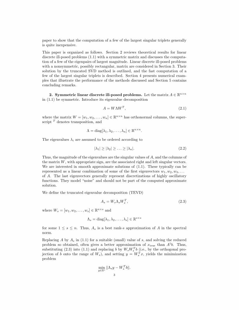
2. Symmetric linear discrete ill-posed problems. Let the matrix A ∈ Rn×n

in (1.1) be symmetric. Introduce its eigenvalue decomposition

A = WΛWT , (2.1)

where the matrix W = [w1, w2, . . . , wn] ∈ Rn×n has orthonormal columns, the super-

script T denotes transposition, and

Λ = diag[λ1, λ2, . . . , λn] ∈ Rn×n.

The eigenvalues λi are assumed to be ordered according to

|λ1| ≥ |λ2| ≥ . . . ≥ |λn|. (2.2)

Thus, the magnitude of the eigenvalues are the singular values of A, and the columns ofthe matrix W , with appropriate sign, are the associated right and left singular vectors.We are interested in smooth approximate solutions of (1.1). These typically can berepresented as a linear combination of some of the first eigenvectors w1, w2, w3, . . .of A. The last eigenvectors generally represent discretizations of highly oscillatoryfunctions. They model “noise” and should not be part of the computed approximatesolution.

We define the truncated eigenvalue decomposition (TEVD)

As = WsΛsWTs , (2.3)

where Ws = [w1, w2, . . . , ws] ∈ Rn×s and

Λs = diag[λ1, λ2, . . . , λs] ∈ Rs×s

for some 1 ≤ s ≤ n. Thus, As is a best rank-s approximation of A in the spectralnorm.

Replacing A by As in (1.1) for a suitable (small) value of s, and solving the reducedproblem so obtained, often gives a better approximation of xtrue than A†b. Thus,substituting (2.3) into (1.1) and replacing b by WsW

Ts b (i.e., by the orthogonal pro-

jection of b onto the range of Ws), and setting y = WTs x, yields the minimization

problem

miny∈Rs

‖Λsy −WTs b‖.

3

Assuming that λs > 0, its solution is given by ys = Λ−1s WT

s b, which yields theapproximate solution

xs = A†sb = WsΛ

−1s WT

s b = Wsys

of (1.1). This approach of computing an approximate solution of (1.1) is known as theTEVD method. It is analogous to the truncated singular value decomposition (TSVD)method for nonsymmetric problems; see [15, 23] or Section 3 for the latter.

There are a variety of ways to determine a suitable value of the truncation indexs, including the discrepancy principle, generalized cross validation, and the L-curvecriterion; see [16, 17, 23, 26, 34] for discussions of these and other methods for choosingan appropriate value of s. We will use the discrepancy principle in the computedexamples of Section 4. This approach to determine s requires that a bound for theerror e in b be available,

‖e‖ ≤ δ,

and prescribes that s ≥ 0 be the smallest integer such that

‖Axs − b‖ ≤ τδ, (2.4)

where τ ≥ 1 is a user-chosen constant independent of δ. We remark that one cancompute the left-hand side without evaluating a matrix-vector product with A byobserving that

‖Axs − b‖ = ‖b−WsWTs b‖.

It can be shown that xs → xtrue as ‖e‖ → 0; see, e.g., [15] for a proof in a Hilbertspace setting. The proof is for the situation when A is nonsymmetric, the eigen-value decomposition (2.1) is replaced by the singular value decomposition, and thetruncated eigenvalue decomposition (2.3) is replaced by a truncated singular valuedecomposition.

Algorithm 1 The Symmetric Lanczos Process

1: Input: A, b 6= 0, ℓ2: Initialize: v1 = b/‖b‖, β1 = 0, v0 = 03: for j = 1, 2, . . . , ℓ do

4: y = Avj − βjvj−1

5: αj = 〈y, vj〉6: y = y − αjvj7: βj+1 = ‖y‖8: if βj+1 = 0 then Stop

9: vj+1 = y/βj+1

10: end

We turn to the computation of the matrices Ws and Λs in (2.3), where we assumethat 1 ≤ s ≪ n. The most popular approaches to compute a few extreme eigenvaluesand associated eigenvectors of a large symmetric matrix are based on the symmetricLanczos process, which is displayed by Algorithm 1; see, e.g., Saad [36] for a thoroughdiscussion of properties of this algorithm. Assume for the moment that the input

4

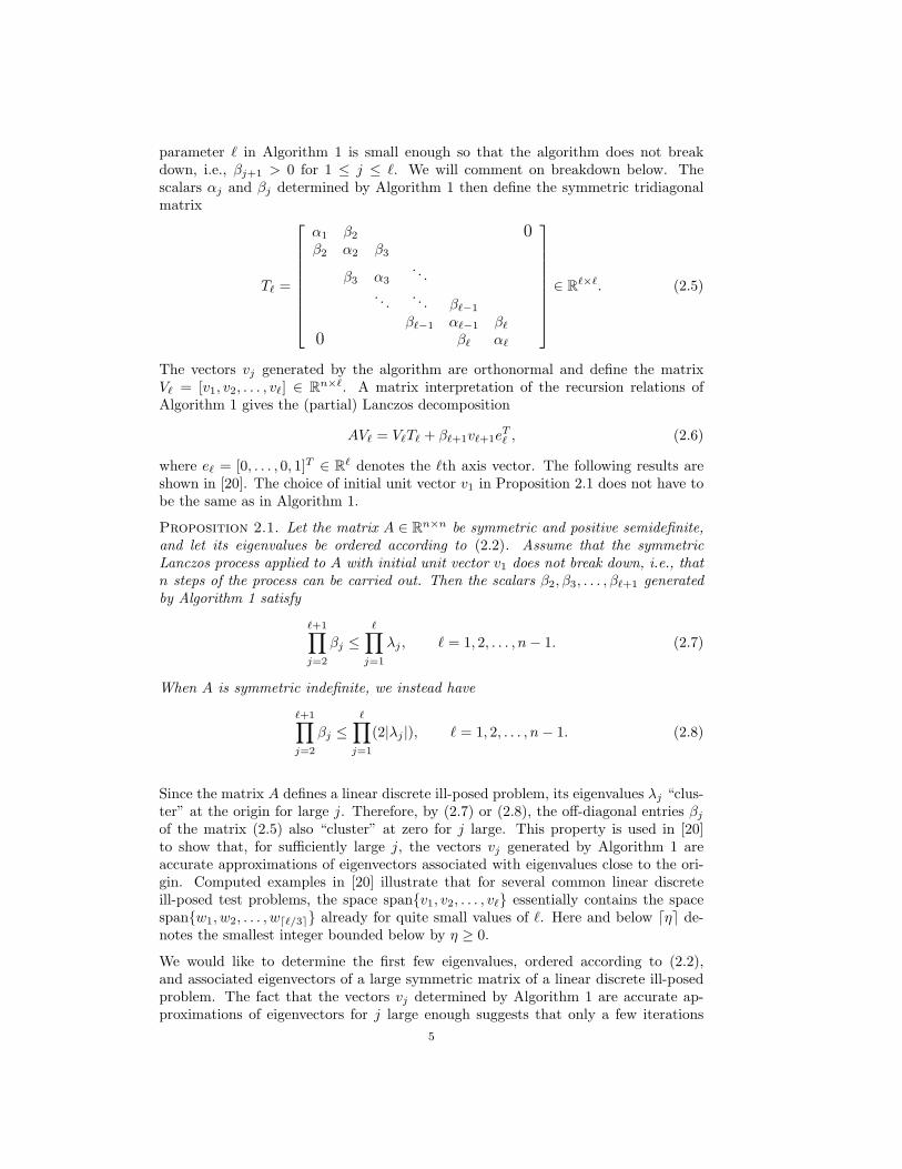
parameter ℓ in Algorithm 1 is small enough so that the algorithm does not breakdown, i.e., βj+1 > 0 for 1 ≤ j ≤ ℓ. We will comment on breakdown below. Thescalars αj and βj determined by Algorithm 1 then define the symmetric tridiagonalmatrix

Tℓ =

α1 β2 0

β2 α2 β3

β3 α3. . .

. . .. . . βℓ−1

βℓ−1 αℓ−1 βℓ

0 βℓ αℓ

∈ Rℓ×ℓ. (2.5)

The vectors vj generated by the algorithm are orthonormal and define the matrixVℓ = [v1, v2, . . . , vℓ] ∈ R

n×ℓ. A matrix interpretation of the recursion relations ofAlgorithm 1 gives the (partial) Lanczos decomposition

AVℓ = VℓTℓ + βℓ+1vℓ+1eTℓ , (2.6)

where eℓ = [0, . . . , 0, 1]T ∈ Rℓ denotes the ℓth axis vector. The following results are

shown in [20]. The choice of initial unit vector v1 in Proposition 2.1 does not have tobe the same as in Algorithm 1.

Proposition 2.1. Let the matrix A ∈ Rn×n be symmetric and positive semidefinite,

and let its eigenvalues be ordered according to (2.2). Assume that the symmetric

Lanczos process applied to A with initial unit vector v1 does not break down, i.e., that

n steps of the process can be carried out. Then the scalars β2, β3, . . . , βℓ+1 generated

by Algorithm 1 satisfy

ℓ+1∏

j=2

βj ≤ℓ∏

j=1

λj , ℓ = 1, 2, . . . , n− 1. (2.7)

When A is symmetric indefinite, we instead have

ℓ+1∏

j=2

βj ≤ℓ∏

j=1

(2|λj |), ℓ = 1, 2, . . . , n− 1. (2.8)

Since the matrix A defines a linear discrete ill-posed problem, its eigenvalues λj “clus-ter” at the origin for large j. Therefore, by (2.7) or (2.8), the off-diagonal entries βj

of the matrix (2.5) also “cluster” at zero for j large. This property is used in [20]to show that, for sufficiently large j, the vectors vj generated by Algorithm 1 areaccurate approximations of eigenvectors associated with eigenvalues close to the ori-gin. Computed examples in [20] illustrate that for several common linear discreteill-posed test problems, the space span{v1, v2, . . . , vℓ} essentially contains the spacespan{w1, w2, . . . , w⌈ℓ/3⌉} already for quite small values of ℓ. Here and below ⌈η⌉ de-notes the smallest integer bounded below by η ≥ 0.

We would like to determine the first few eigenvalues, ordered according to (2.2),and associated eigenvectors of a large symmetric matrix of a linear discrete ill-posedproblem. The fact that the vectors vj determined by Algorithm 1 are accurate ap-proximations of eigenvectors for j large enough suggests that only a few iterations

5

with an implicitly restarted symmetric Lanczos method, such as the methods de-scribed in [3, 4, 13, 39], are required. These methods compute a sequence of Lanczosdecompositions of the form (2.6) with different initial vectors. Let v1 be the initialvector in the presently available Lanczos decomposition (2.6). An initial vector forthe next Lanczos decomposition is determined by applying a polynomial filter q(A)to v1 to obtain the initial vector q(A)v1/‖q(A)v1‖ of the next Lanczos decomposition.The computation of q(A)v1 is carried out without evaluating additional matrix-vectorproducts with A. The implementations [3, 4, 13, 39] use different polynomials q. Itis the purpose of the polynomial filter q(A) to damp components of unwanted eigen-vectors in the vector v1. We are interested in damping components of eigenvectorsassociated with eigenvalues of small magnitude. The implicitly restarted symmetricLanczos method was first described in [13, 39]. We will use the implementation [3, 4]of the implicitly restarted symmetric block Lanczos method with block size one incomputations reported in Section 4.

We remark that there are several reasons for solving linear discrete ill-posed problems(1.1) with a symmetric matrix A by the TEVD method. One of them is that thesingular values of A, i.e., the magnitude of the eigenvalues of A, provide importantinformation about the matrix A and thereby about properties of the linear discrete ill-posed problem (1.1). For instance, the decay rate of the singular values with increasingindex is an important property of a linear discrete ill-posed problem. Problems whosesingular values decay quickly are referred to as severely ill-posed. Moreover, thetruncated eigendecomposition (2.3) may furnish an economical storage format for theimportant part of the matrix A. Large matrices A that stem from the discretizationof a Fredholm integral equation of the first kind are generally dense, however, itoften suffices to store only a few of its largest eigenpairs. Storage of these eigenpairstypically requires much less computer memory than storage of the matrix A.

We finally comment on the situation when Algorithm 1 breaks down. This happenswhen some coefficient βj+1 vanishes. We then have determined an invariant subspaceof A. If this subspace contains all the desired eigenvectors, then we compute anapproximation of xtrue in this subspace. Otherwise, we restart Algorithm 1 with aninitial vector that is orthogonal to the invariant subspace already found. Since theoccurrence of breakdown is rare, we will not dwell on this topic further.

3. Nonsymmetric linear discrete ill-posed problems. This section is con-cerned with the solution of linear discrete ill-posed problems (1.1) with a large non-symmetric matrix A ∈ R

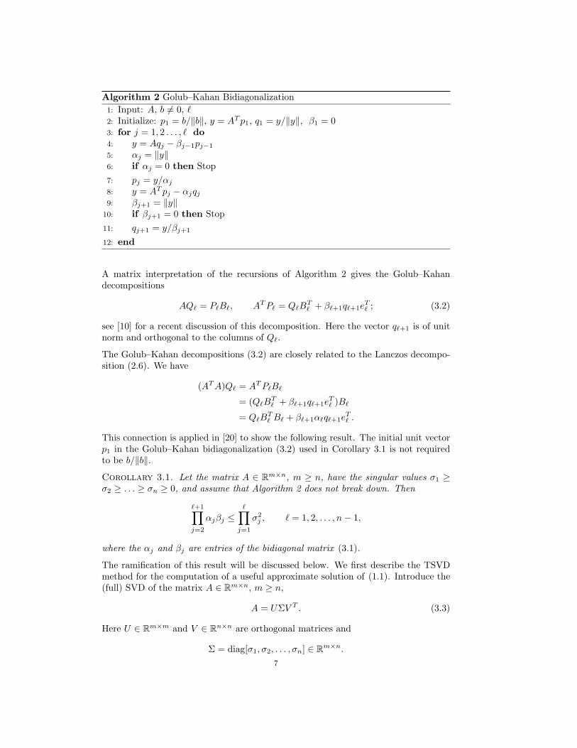
m×n. Such a matrix can be reduced to a small matrix byapplication of a few steps of Golub–Kahan bidiagonalization. This is described byAlgorithm 2. The algorithm is assumed not to break down.

Using the vectors pj and qj determined by Algorithm 2, we define the matrices Pℓ =[p1, p2, . . . , pℓ] ∈ R

m×ℓ and Qℓ = [q1, q2, . . . , qℓ] ∈ Rn×ℓ with orthonormal columns.

The scalars αj and βj computed by the algorithm define the bidiagonal matrix

Bℓ =

α1 β2 0

α2 β3

α3 β4

. . .. . .

αℓ−1 βℓ

0 αℓ

∈ Rℓ×ℓ. (3.1)

6

Algorithm 2 Golub–Kahan Bidiagonalization

1: Input: A, b 6= 0, ℓ2: Initialize: p1 = b/‖b‖, y = AT p1, q1 = y/‖y‖, β1 = 03: for j = 1, 2 . . . , ℓ do

4: y = Aqj − βj−1pj−1

5: αj = ‖y‖6: if αj = 0 then Stop

7: pj = y/αj

8: y = AT pj − αjqj9: βj+1 = ‖y‖

10: if βj+1 = 0 then Stop

11: qj+1 = y/βj+1

12: end

A matrix interpretation of the recursions of Algorithm 2 gives the Golub–Kahandecompositions

AQℓ = PℓBℓ, ATPℓ = QℓBTℓ + βℓ+1qℓ+1e

Tℓ ; (3.2)

see [10] for a recent discussion of this decomposition. Here the vector qℓ+1 is of unitnorm and orthogonal to the columns of Qℓ.

The Golub–Kahan decompositions (3.2) are closely related to the Lanczos decompo-sition (2.6). We have

(ATA)Qℓ = ATPℓBℓ

= (QℓBTℓ + βℓ+1qℓ+1e

Tℓ )Bℓ

= QℓBTℓ Bℓ + βℓ+1αℓqℓ+1e

Tℓ .

This connection is applied in [20] to show the following result. The initial unit vectorp1 in the Golub–Kahan bidiagonalization (3.2) used in Corollary 3.1 is not requiredto be b/‖b‖.Corollary 3.1. Let the matrix A ∈ R

m×n, m ≥ n, have the singular values σ1 ≥σ2 ≥ . . . ≥ σn ≥ 0, and assume that Algorithm 2 does not break down. Then

ℓ+1∏

j=2

αjβj ≤ℓ∏

j=1

σ2j , ℓ = 1, 2, . . . , n− 1,

where the αj and βj are entries of the bidiagonal matrix (3.1).

The ramification of this result will be discussed below. We first describe the TSVDmethod for the computation of a useful approximate solution of (1.1). Introduce the(full) SVD of the matrix A ∈ R

m×n, m ≥ n,

A = UΣV T . (3.3)

Here U ∈ Rm×m and V ∈ R

n×n are orthogonal matrices and

Σ = diag[σ1, σ2, . . . , σn] ∈ Rm×n.

7

The singular values are ordered according to

σ1 ≥ σ2 ≥ · · · ≥ σr > σr+1 = · · · = σn = 0,

where r is the rank of A. Let the matrix Us ∈ Rm×s be made up of the first s columns

of U , where 1 ≤ s ≤ r. Similarly, let Vs ∈ Rn×s consist of the first s columns of V , and

let Σs denote the leading s× s principal submatrix of Σ. This gives the TSVD

As = UsΣsVTs . (3.4)

Note that As is a best rank-s approximation of A in the spectral norm. The TSVDapproximate solutions of (1.1) are given by

xs = A†sb = VsΣ

−1s UT

s b, 1 ≤ s ≤ r. (3.5)

The discrepancy principle prescribes that the truncation index s be chosen as smallas possible so that (2.4) holds with xs given by (3.5); see, e.g., [15, 23, 31] for detailsof this approach to determine approximations of xtrue.

It follows from Corollary 3.1 and the fact that the singular values of A cluster atthe origin, that the columns qj of the matrix Qℓ in (3.2) for large j are accurateapproximations of eigenvectors of ATA; see [20] for details. This suggests that theimplicitly restarted Golub–Kahan bidiagonalization methods described in [5, 6, 7, 8],for many matrices A that stem from the discretization of a linear ill-posed problem,only require fairly few matrix-vector product evaluations to determine a truncatedsingular value decomposition (3.4) with s fairly small. Illustrations are presented inthe following section. We remark that the solution of linear discrete ill-posed problems(1.1) with a nonsymmetrix matrix by the TSVD method is of interest for the samereasons as the TEVD is attractive to use for the solution of linear discrete ill-posedproblems with a symmetric matrix A; see the end of Section 2 for a discussion.

4. Computed examples. The main purpose of the computed examples is toillustrate that a few of the largest singular triplets of a large matrix A (or a few of thelargest eigenpairs when A is symmetric) can be computed quite inexpensively whenA defines a linear discrete ill-posed problem (1.1). All computations are carried outusing MATLAB R2012a with about 15 significant decimal digits. A Sony computerrunning Windows 10 with 4 GB of RAM was used. MATLAB codes for determiningthe discrete ill-posed problems in the computed examples stem from RegularizationTools by Hansen [24]. When not explicitly stated otherwise, the matrices A areobtained by discretizing a Fredholm integral equation of the first kind, and are squareand of order n = 500. For some examples finer discretizations, resulting in largermatrices, are used.

The first few examples illustrate that the number of matrix-vector product evaluationsrequired to compute the k eigenpairs of largest magnitude or the k largest singulartriplets of a large matrix obtained by the discretization of an ill-posed problem isa fairly small multiple of k. The computations for a symmetric matrix A can beorganized in two ways: We use the code irbleigs described in [3, 4] or the code irbla

presented in [6]. The former code has an input parameter that specifies whether thek largest or the k smallest eigenvalues are to be computed. Symmetric semidefinitematrices A may only require one call of irbleigs to determine the desired eigenpairs,while symmetric indefinite matrices require at least one call for computing a few of the

8

largest eigenvalues and associated eigenvectors, and at least one call for computinga few of the smallest eigenvalues and associated eigenvectors. We have found thatthe irbla code, which determines a few of the largest singular values and associatedsingular vectors can be competitive with irbleigs for symmetric indefinite matrices,because it is possible to compute all the required eigenpairs (i.e., singular triplets)with only one call of irbla.

We use the MATLAB code irbleigs [4] with block size one to compute the k eigenvaluesof largest magnitude of a large symmetric matrix A. The code carries out ⌈2.5k⌉Lanczos steps between restarts; i.e., a sequence of Lanczos decompositions (2.6) withℓ = ⌈2.5k⌉ are computed with different initial vectors v1 until the k desired eigenvaluesand associated eigenvectors have been determined with specified accuracy. The defaultcriterion for accepting computed approximate eigenpairs is used, i.e., a computedapproximate eigenpair {λj , wj}, with ‖wj‖ = 1, is accepted as an eigenpair of Aif

‖Awj − wj λj‖ ≤ εη(A), j = 1, 2, . . . , k, (4.1)

where η(A) is an easily computable approximation of ‖A‖ and ε = 10−6. The irbleigs

code uses a computed approximation of the largest singular value of A as η(A).

Table 1

foxgood test problem.

Number of desired Size of the largest Number ofeigenpairs k tridiagonal matrix matrix-vector products

5 ⌈2.5k⌉ 2410 ⌈2.5k⌉ 3215 ⌈2.5k⌉ 3220 ⌈2.5k⌉ 4025 ⌈2.5k⌉ 50

Example 4.1. We illustrate the performance of the irbleigs method [4] when appliedto a discretization of the Fredholm integral equation of the first kind

∫ 1

0

(s2 + t2

)1/2x(t)dt =

1

3(1 + s2)

3

2 − s3, 0 ≤ s ≤ 1,

with solution x(t) = t. This equation is discussed by Fox and Goodwin [18]. We usethe function foxgood from [24] to determine a discretization by a Nystrom method.This gives a symmetric indefinite matrix A ∈ R

500×500. Its eigenvalues cluster at zeroand the computed condition number κ(A) = ‖A‖‖A†‖ obtained with the MATLABfunction cond is 3.8×1019. Thus, the matrix is numerically singular. Table 1 displaysthe average number of matrix-vector product evaluations required by irbleigs over 1000runs rounded to the closest integer when applied as described above to compute thek eigenpairs of largest magnitude for k = 5, 10, . . . , 25. The number of matrix-vectorproduct evaluations is seen to grow about linearly with k for the larger k-values. Sinceirbleigs chooses the initial vector in the first Lanczos decomposition computed to bea unit random vector, the number of matrix-vector product evaluations may varysomewhat between different calls of irbleigs.

9

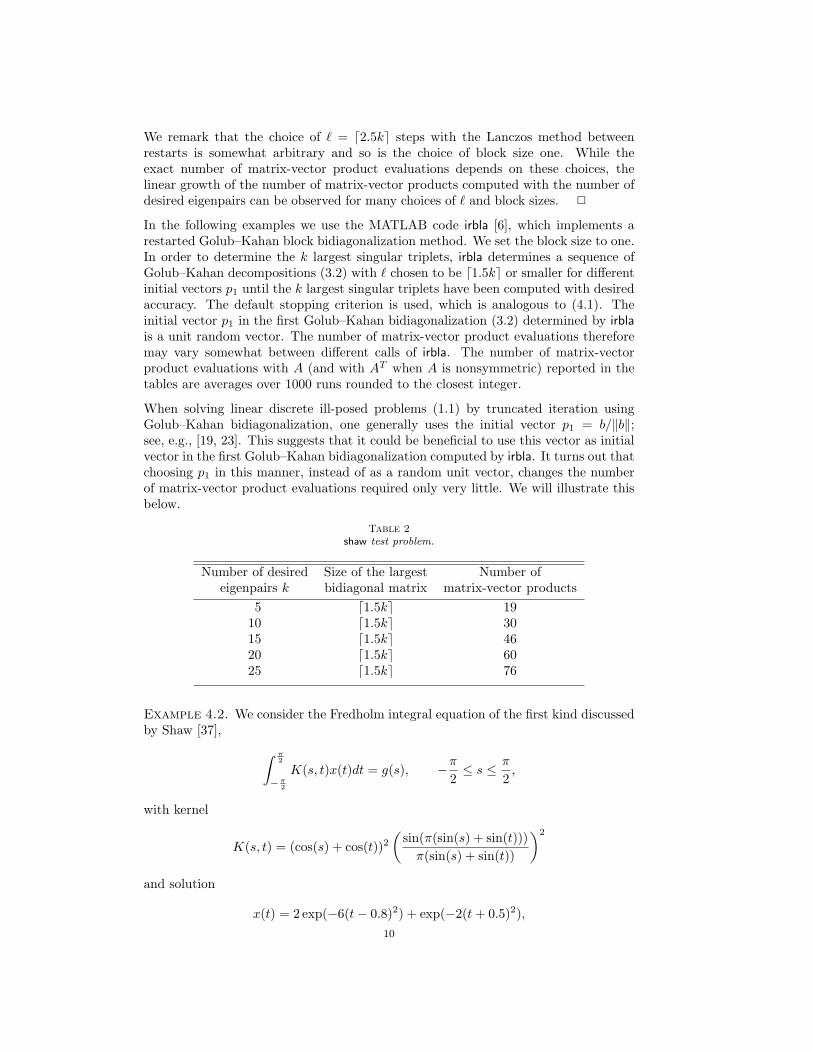
We remark that the choice of ℓ = ⌈2.5k⌉ steps with the Lanczos method betweenrestarts is somewhat arbitrary and so is the choice of block size one. While theexact number of matrix-vector product evaluations depends on these choices, thelinear growth of the number of matrix-vector products computed with the number ofdesired eigenpairs can be observed for many choices of ℓ and block sizes. ✷

In the following examples we use the MATLAB code irbla [6], which implements arestarted Golub–Kahan block bidiagonalization method. We set the block size to one.In order to determine the k largest singular triplets, irbla determines a sequence ofGolub–Kahan decompositions (3.2) with ℓ chosen to be ⌈1.5k⌉ or smaller for differentinitial vectors p1 until the k largest singular triplets have been computed with desiredaccuracy. The default stopping criterion is used, which is analogous to (4.1). Theinitial vector p1 in the first Golub–Kahan bidiagonalization (3.2) determined by irbla

is a unit random vector. The number of matrix-vector product evaluations thereforemay vary somewhat between different calls of irbla. The number of matrix-vectorproduct evaluations with A (and with AT when A is nonsymmetric) reported in thetables are averages over 1000 runs rounded to the closest integer.

When solving linear discrete ill-posed problems (1.1) by truncated iteration usingGolub–Kahan bidiagonalization, one generally uses the initial vector p1 = b/‖b‖;see, e.g., [19, 23]. This suggests that it could be beneficial to use this vector as initialvector in the first Golub–Kahan bidiagonalization computed by irbla. It turns out thatchoosing p1 in this manner, instead of as a random unit vector, changes the numberof matrix-vector product evaluations required only very little. We will illustrate thisbelow.

Table 2

shaw test problem.

Number of desired Size of the largest Number ofeigenpairs k bidiagonal matrix matrix-vector products

5 ⌈1.5k⌉ 1910 ⌈1.5k⌉ 3015 ⌈1.5k⌉ 4620 ⌈1.5k⌉ 6025 ⌈1.5k⌉ 76

Example 4.2. We consider the Fredholm integral equation of the first kind discussedby Shaw [37],

∫ π2

−π2

K(s, t)x(t)dt = g(s), −π

2≤ s ≤ π

2,

with kernel

K(s, t) = (cos(s) + cos(t))2(sin(π(sin(s) + sin(t)))

π(sin(s) + sin(t))

)2

and solution

x(t) = 2 exp(−6(t− 0.8)2) + exp(−2(t+ 0.5)2),

10

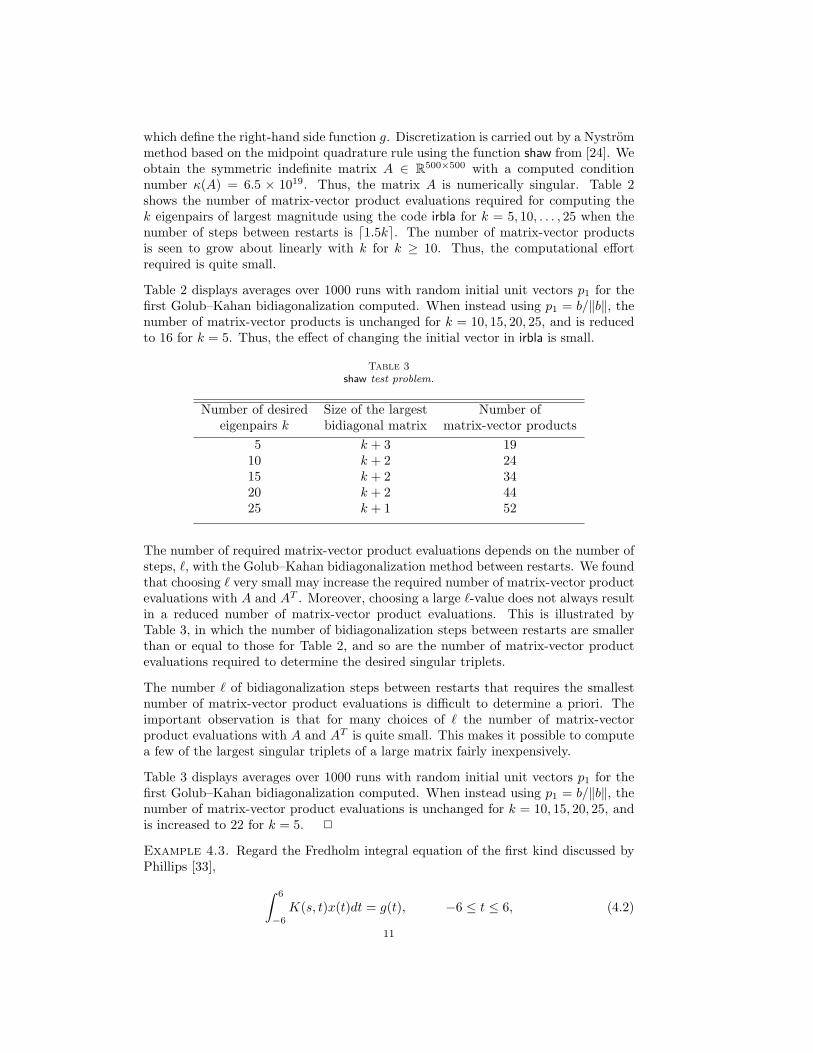
which define the right-hand side function g. Discretization is carried out by a Nystrommethod based on the midpoint quadrature rule using the function shaw from [24]. Weobtain the symmetric indefinite matrix A ∈ R

500×500 with a computed conditionnumber κ(A) = 6.5 × 1019. Thus, the matrix A is numerically singular. Table 2shows the number of matrix-vector product evaluations required for computing thek eigenpairs of largest magnitude using the code irbla for k = 5, 10, . . . , 25 when thenumber of steps between restarts is ⌈1.5k⌉. The number of matrix-vector productsis seen to grow about linearly with k for k ≥ 10. Thus, the computational effortrequired is quite small.

Table 2 displays averages over 1000 runs with random initial unit vectors p1 for thefirst Golub–Kahan bidiagonalization computed. When instead using p1 = b/‖b‖, thenumber of matrix-vector products is unchanged for k = 10, 15, 20, 25, and is reducedto 16 for k = 5. Thus, the effect of changing the initial vector in irbla is small.

Table 3

shaw test problem.

Number of desired Size of the largest Number ofeigenpairs k bidiagonal matrix matrix-vector products

5 k + 3 1910 k + 2 2415 k + 2 3420 k + 2 4425 k + 1 52

The number of required matrix-vector product evaluations depends on the number ofsteps, ℓ, with the Golub–Kahan bidiagonalization method between restarts. We foundthat choosing ℓ very small may increase the required number of matrix-vector productevaluations with A and AT . Moreover, choosing a large ℓ-value does not always resultin a reduced number of matrix-vector product evaluations. This is illustrated byTable 3, in which the number of bidiagonalization steps between restarts are smallerthan or equal to those for Table 2, and so are the number of matrix-vector productevaluations required to determine the desired singular triplets.

The number ℓ of bidiagonalization steps between restarts that requires the smallestnumber of matrix-vector product evaluations is difficult to determine a priori. Theimportant observation is that for many choices of ℓ the number of matrix-vectorproduct evaluations with A and AT is quite small. This makes it possible to computea few of the largest singular triplets of a large matrix fairly inexpensively.

Table 3 displays averages over 1000 runs with random initial unit vectors p1 for thefirst Golub–Kahan bidiagonalization computed. When instead using p1 = b/‖b‖, thenumber of matrix-vector product evaluations is unchanged for k = 10, 15, 20, 25, andis increased to 22 for k = 5. ✷

Example 4.3. Regard the Fredholm integral equation of the first kind discussed byPhillips [33],

∫ 6

−6

K(s, t)x(t)dt = g(t), −6 ≤ t ≤ 6, (4.2)

11

Table 4

phillips test problem.

Number of desired Size of the largest Number ofeigenpairs k bidiagonal matrix matrix-vector products

5 ⌈1.5k⌉ 2210 ⌈1.5k⌉ 3615 ⌈1.5k⌉ 4620 ⌈1.5k⌉ 6025 ⌈1.5k⌉ 76

where the solution x(t), kernel K(s, t), and right-hand side g(s) are given by

x(t) =

{1 + cos

(πt3

), |t| < 3,

0, |t| ≥ 3,

K(s, t) = x(s− t),

g(s) = (6− |s|)(1 +

1

2cos

(πs3

))+

9

2πsin

(π|s|3

).

The integral equation is discretized by a Galerkin method using the MATLAB functionphillips from [24]. The matrix A ∈ R

500×500 produced is symmetric and indefinitewith many eigenvalues close to zero. It is ill-conditioned with condition numberκ(A) = 1.7× 109.

Table 4 displays the number of matrix-vector product evaluations required to com-pute the k eigenpairs of largest magnitude (i.e., the k largest singular triplets) fork = 5, 10, . . . , 25 by irbla. A random unit vector p1 is used as initial vector for the firstGolub–Kahan bidiagonalization computed by irbla and the number of matrix-vectorproduct evaluations are averages over 1000 runs. The number of matrix-vector prod-uct evaluations is seen to grow about linearly with k for k ≥ 10. If instead p1 = b/‖b‖is used as initial vector for the first Golub–Kahan bidiagonalization computed by ir-

bla, the number of matrix-vector product evaluations is the same for k = 5, 10, . . . , 25.Thus, the choice of initial vector is not important.

The number of required matrix-vector product evaluations is quite insensitive to howfinely the integral equations (4.2) is discretized for all fine enough discretizations.For instance, when the integral equation is discretized by a Galerkin method usingthe MATLAB function phillips from [24] to obtain a matrix A ∈ R

5000×5000 and theinitial vector for the first Golub–Kahan bidiagonalization computed by irbla is chosento be p1 = b/‖b‖, the number of required matrix-vector product evaluations is thesame as for A ∈ R

500×500. We conclude that the computational expense to com-pute a truncated singular value decomposition of A is modest also for large matrices.✷

The following examples are concerned with nonsymmetric matrices. The k largestsingular triplets are computed with the irbla code [6] using block size one.

Example 4.4. The Fredholm integral equation of the first kind

∫ π

0

exp(s cos t)x(t)dt = 2sin s

s, 0 ≤ s ≤ π

2,

12

Table 5

baart test problem.

Number of desired Size of the largest Number ofsingular triplets k bidiagonal matrix matrix-vector products

5 ⌈1.5k⌉ 1610 ⌈1.5k⌉ 3015 ⌈1.5k⌉ 4620 ⌈1.5k⌉ 6025 ⌈1.5k⌉ 76

is discussed by Baart [2]. It has the solution x(t) = sin(t). The integral equationis discretized by a Galerkin method with piece-wise constant test and trial functionsusing the function baart from [24]. This gives a nonsymmetric matrix A ∈ R

500×500.Its computed condition number is κ(A) = 8.9 × 1018. Table 5 shows the number ofrequired matrix-vector product evaluations to grow roughly linearly with the numberof desired largest singular triplets. Both the initial vector p1 = b/‖b‖ and the averageover 1000 runs with a random unit initial vector p1 for the initial Golub–Kahanbidiagonalization computed by irbla yield the same entries of the last column.

Table 6

baart test problem.

Number of desired Size of the largest Number ofsingular triples k bidiagonal matrix matrix-vector products

5 k + 2 1410 k + 1 2215 k + 1 3220 k + 1 4225 k + 1 52

Table 6 is analogous to Table 5. Only the number of steps ℓ between restarts ofGolub–Kahan bidiagonalization differs. They are smaller in Table 6 than in Table 5and so are the required number of matrix-vector product evaluations with A and AT .Also in Table 6 the number of matrix-vector products needed is seen to grow aboutlinearly with k. The initial vector p1 = b/‖b‖ and the average over 1000 runs with arandom unit initial vector p1 for the first Golub–Kahan bidiagonalization computedby irbla yield the same entries in the last column of Table 6. ✷

Example 4.5. The inverse Laplace transform,

∫ ∞

0

exp(−st)x(t)dt =16

(2s+ 1)3, s ≥ 0, (4.3)

is discretized by means of Gauss–Laguerre quadrature using the MATLAB functioni laplace from [24]. The nonsymmetric matrix A ∈ R

500×500 so obtained is numericallysingular. The solution of (4.3) is x(t) = t2 exp

(− t

2

). Table 7 displays the number of

matrix-vector product evaluations required to compute the k largest singular triples.This number is seen to grow about linearly with k. Therefore, the computationaleffort is quite small. The initial vector p1 = b/‖b‖ and the average over 1000 runs

13

Table 7

Inverse Laplace transform test problem.

Number of desired Size of the largest Number ofsingular triplets k bidiagonal matrix matrix-vector products

5 ⌈1.5k⌉ 2210 ⌈1.5k⌉ 3015 ⌈1.5k⌉ 4620 ⌈1.5k⌉ 6025 ⌈1.5k⌉ 76

with a random unit initial vector p1 for the initial Golub–Kahan bidiagonalizationcomputed by irbla yield the same entries in the last column of Table 7. ✷

Table 8

Relative errors and number of matrix-vector products, δ = 10−2. The initial vector for the first

Golub–Kahan bidiagonalization computed by irbla is a unit random vector.

Problem s MVP Epsvd Etsvd Es

shaw 7 22 8.23×10−15 5.06×10−2 5.06×10−2

phillips 7 22 7.77×10−9 2.53×10−2 2.53×10−2

baart 3 10 7.94×10−8 1.67×10−1 1.67×10−1

i laplace 7 22 3.67×10−7 2.24×10−1 2.24×10−1

Table 9

Relative errors and number of matrix-vector products, δ = 10−2. The initial vector for the first

Golub–Kahan bidiagonalization computed by irbla is b/‖b‖.

Problem s MVP Epsvd Etsvd Es

shaw 7 22 8.29×10−15 4.97×10−2 4.97×10−2

phillips 7 22 9.25×10−10 2.50×10−2 2.50×10−2

baart 3 10 1.15×10−9 1.68×10−1 1.68×10−1

i laplace 7 22 1.00×10−8 2.24×10−1 2.24×10−1

Example 4.6. This example compares the quality of approximate solutions of lineardiscrete ill-posed problems computed by truncated singular value decomposition. Thedecompositions are determined as described in this paper as well as by computing thefull SVD (3.3) with the MATLAB function svd. It is the aim of this example to showthat the decompositions computed in these ways yield approximations of xtrue of thesame quality. We use the discrepancy principle (2.4) to determine the truncationindex s.

The number of matrix-vector product evaluations used to compute approximations ofxtrue depends on the number of singular triplets required to satisfy the discrepancyprinciple. The latter number typically increases as the error in the vector b in (1.1)decreases because then the least-squares problem has to be solved more accurately. Inrealistic applications, one would first compute the ℓ largest singular triplets, for someuser-chosen value of ℓ, and if it turns out that additional singular triplets are requiredto satisfy the discrepancy principle, then one would determine the next, say, ℓ largest

14

Table 10

Relative errors and number of matrix-vector products, δ = 10−4. The initial vector for the first

Golub–Kahan bidiagonalization computed by irbla is b/‖b‖.

Problem s MVP Epsvd Etsvd Es

shaw 9 28 5.01×10−14 3.21×10−2 3.21×10−2

phillips 12 42 3.33×10−8 4.23×10−3 4.23×10−3

baart 4 12 1.71×10−10 1.15×10−1 1.15×10−1

i laplace 12 40 5.46×10−13 1.71×10−1 1.71×10−1

Table 11

Relative errors and number of matrix-vector products, δ = 10−6. The initial vector for the first

Golub–Kahan bidiagonalization computed by irbla is b/‖b‖.

Problem s MVP Epsvd Etsvd Es

shaw 10 30 1.22×10−12 1.94×10−2 1.94×10−2

phillips 27 82 2.47×10−13 7.99×10−4 7.99×10−4

baart 5 16 1.67×10−12 5.26×10−2 5.26×10−2

i laplace 18 54 4.32×10−12 1.43×10−1 1.43×10−1

singular triplets, etc. This approach may require the evaluation of somewhat morematrix-vector products than if all required largest singular triplets were computedtogether. Conversely, if only the ℓ/2 largest singular triplets turn out to be neededto satisfy the discrepancy principle, then the number of matrix-vector products canbe reduced by initially computing only these triplets instead of the ℓ largest singulartriplets.

To reduce the influence on the number of matrix-vector products required by thesomewhat arbitrary choice of the initial number of largest singular triplets to be com-puted, we proceed as follows. We first compute the SVD (3.3) using the MATLABfunction svd and then determine the smallest truncation index s so that the discrep-ancy principle (2.4) holds. We denote the approximation of xtrue so determined byxtsvd. Then we use irbla to compute the s largest singular triplets of A. Several tablescompare the quality of the so computed approximations of xtrue in different ways.The quantity

Epsvd =‖xs − xtsvd‖

‖xtsvd‖

shows the relative difference between the approximate solution xtsvd and the approx-imate solution xs determined by computing a truncated singular value decomposi-tion (3.4) of the matrix A using the irbla method with the number of Golub–Kahanbidiagonalization steps between restarts set to ⌈1.5s⌉. We also display the relativedifference

Etsvd =‖xtsvd − xtrue‖

‖xtrue‖,

which shows how well the approximate solution determined by the full singular valuedecomposition approximates the desired solution xtrue. The analogous relative differ-

15

ence

Es =‖xs − xtrue‖

‖xtrue‖

shows how well the approximate solution determined by the truncated singular valuedecomposition approximates xtrue.

Tables 8-11 report results for three noise levels δ = ‖e‖/‖btrue‖ (δ = 10−t for t =2, 4, 6) and τ = 1 in (2.4). The error vector e models white Gaussian noise. Thus,given the vector btrue, which is generated by the MATLAB function that determinesthe matrix A, a vector e that models white Gaussian noise is added to btrue to obtainthe error-contaminated vector b; cf. (1.2). The vector e is scaled to correspond to a

prescribed noise level δ. We generate this additive noise vector, e, with

e := e ‖btrue‖δ√n,

where e ∈ R500 is a random vector whose entries are from a normal distribution with

mean zero and variance one.

For Tables 9-11, the initial vector for the first Golub–Kahan bidiagonalization com-puted by irbla is chosen to be p1 = b/‖b‖. This choice is quite natural, because wewould like to solve least-squares problems (1.1) with data vector b. The table columnswith heading “MVP” display the number of matrix-vector product evaluations re-quired by irbla to compute the truncated singular value decomposition required tosatisfy the discrepancy principle. Table 8 shows averages over 1000 runs with randomunit initial vectors p1 for the first Golub–Kahan bidiagonalization computed by irbla.The entries of this table and Table 9 are quite close. The closeness of correspondingentries also can be observed for smaller noise levels. We therefore omit to displaytables analogous to Table 8 for smaller noise levels.

Tables 8-11 show the computed approximate solutions determined by using irbla togive as good approximations of xtrue as the approximate solutions xtsvd computedwith the aid of the full SVD (3.3), while being much cheaper to evaluate. ✷

Example 4.7. The LSQR iterative method for the solution of the minimizationproblem (1.1) determines partial bidiagonalizations of A with initial vector b/‖b‖.These bidiagonalizations are closely related to the bidiagonalizations (3.2); see, e.g.,[10, 21] for details. In the ith step, LSQR computes an approximate solution xi in theKrylov subspace Ki(A

TA,AT b) = span{AT b, (ATA)AT b, . . . , (ATA)i−1AT b}. Thisapproximate solution satisfies

‖Axi − b‖ = minx∈Ki(ATA,AT b)

‖Ax− b‖.

The number of steps i is determined by the discrepancy principle, i.e., i is chosen to bethe smallest integer such that the computed approximate solution xi satisfies

‖Axi − b‖ ≤ τδ;

c.f. (2.4). Details on the application of LSQR with the discrepancy principle arediscussed in, e.g., [15, 19, 23].

16

This example considers the situation when there are several data vectors, i.e., wewould like to solve

minxj∈Rn

‖Axj − bj‖, j = 1, 2, . . . , ℓ. (4.4)

We let the matrix A ∈ R500×500 be determined by one of the functions in Regular-

ization Tools [24] already used above. This function also determines the error-freedata vector btrue,1 ∈ R

500. The remaining error-free data vectors btrue,j ∈ R500 are

obtained by choosing discretizations xtrue,j , j = 2, 3, . . . , ℓ, of functions of the formα sin(βt)+ γ, α cos(βt)+ γ, α arctan(βt)+ γ, and αt2 +βt+ γ, where α, β, and γ arerandomly generated scalars, and letting btrue,j = Axtrue,j . A “noise” vector ej ∈ R

500

with normally distributed random entries with zero mean is added to each data vectorbtrue,j to determine an error-contaminated data vector bj ; see (1.2). The noise-vectorsej are scaled to correspond to a specified noise level. This is simulated with

ej := ej ‖btrue,j‖δ√n,

where δ is the noise level, and ej ∈ Rn is a vector, whose elements are normally

distributed random numbers with mean zero and variance one.

Assume that the data vectors are available sequentially. Then the linear discreteill-posed problems (4.4) can be solved one by one by

(A) applying the LSQR iterative method to each one of the ℓ linear discrete ill-posed problems (4.4). The iterations for each system are terminated by thediscrepancy principle. Since the data vectors bj are distinct, each one ofthese vectors requires that a new partial Golub–Kahan bidiagonalization becomputed, and by

(B) computing one TSVD of the matrix A by the irblamethod, and then using thisdecomposition to determine an approximate solution of each one of the prob-lems (4.4). The discrepancy principle is applied to compute the approximatesolution of each least-squares problem. Thus, we determine the parameter sin (3.5) as large as possible so that (2.4) holds with τ = 1.

Seed methods furnish another solution approach that is commonly applied when seek-ing to solve several linear systems of equations with the same matrix and differentright-hand sides that stem from the discretization of well-posed problems, such asDirichlet boundary value problems for an elliptic partial differential equations; see,e.g., [1, 35, 38] and references therein. A Golub–Kahan bidiagonalization-based seedmethod applied to the solution of the ℓ > 1 least-squares problems (4.4) could pro-ceed as follows. First one computes a partial Golub–Kahan bidiagonalization for theleast-squares problem with one of the data vectors, say b1, and then uses this bidiago-nalization to solve all the remaining least-squares problems (4.4). The Golub–Kahanbidiagonalization is determined by the matrix A and the initial vector p1 = b1/‖b1‖.However, while Golub–Kahan bidiagonalization is a well-established technique forsolving linear discrete ill-posed problems, see, e.g., [19, 23], available theory requiresthe initial vector p1 in the decomposition (3.2) to be the data vector normalized tohave unit norm; see, e.g., Hanke [22]. This requirement is satisfied by method (A),but not by seed methods. Due to the lack of theoretical support, we will not applyseed methods in this example.

17

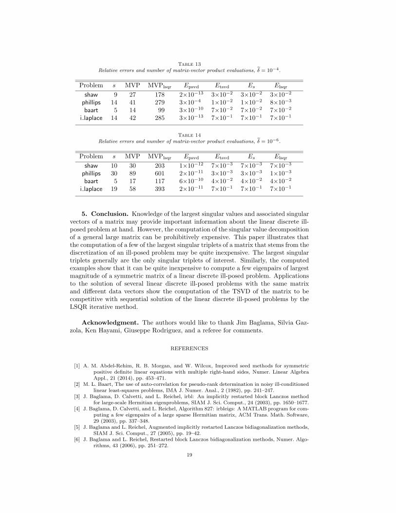
Tables 12-14 compare the number of matrix-vector products required by the ap-proaches (A) and (B) for ℓ = 10 and noise-contaminated data vectors bj corresponding

to the noise levels δ = 10−2, δ = 10−4, and δ = 10−6. For each noise level, 100 noise-contaminated data vectors bj are generated for each 1 ≤ j ≤ ℓ. The initial Golub–Kahan bidiagonalization determined by irbla uses the initial vector p1 = b1/‖b1‖. Thetables display averages over the realizations of the noise-contaminated data vectorsbj . Similarly as in Example 4.5, the number of matrix-vector product evaluationsrequired by the method of this paper depends on the initial choice of the number ofsingular triplets to be computed. To simplify the comparison, we assume this numberto be known. The competitiveness of the method of this paper is not significantlyaffected by this assumption; it is straightforward to compute more singular triplets ifthe initial number of computed triplets is found to be too small to satisfy the discrep-ancy principle. To avoid that round-off errors introduced during the computationswith LSQR delay convergence, Golub–Kahan bidiagonalization is carried out withreorthogonalization; see [23] for a discussion of the role of round-off errors on theconvergence.

The columns of Tables 12-14 are labeled similarly as in the previous examples. Theerror in the computed solutions is the maximum for the errors for each one of the least-squares problems (4.4). The columns labeled MVPlsqr show the average numbers ofmatrix-vector product evaluations required by LSQR, and the columns denoted byElsqr shows the relative error in the approximate solution determined by the LSQRalgorithm, xlsqr, i.e.,

Elsqr =‖xlsqr − xtrue‖

‖xtrue‖.

Tables 12-14 show the method of the present paper to require significantly fewermatrix-vector product evaluations than repeated application of LSQR. For large-scaleproblems, the dominating computational effort of these methods is the evaluation ofmatrix-vector products with A and AT . Similarly as in Example 4.2, the number ofmatrix-vector product evaluations does not change significantly with the fineness ofthe discretization, i.e., with the size of the matrix A determined by the functions in[24].

Finally, we remark that, while the present example uses the discrepancy principleto determine the parameter s in (3.5) and the number of LSQR iterations, othertechniques also can be used for these purposes, such as methods discussed in [16, 17,23, 26, 34]. The results would be fairly similar. ✷

Table 12

Relative errors and number of matrix-vector product evaluations, δ = 10−2.

Problem s MVP MVPlsqr Epsvd Etsvd Es Elsqr

shaw 6 20 133 3×10−6 2×10−1 2×10−1 1×10−1

phillips 7 22 152 1×10−6 7×10−2 7×10−2 6×10−2

baart 3 10 71 2×10−8 1×10−1 1×10−1 1×10−1

i laplace 8 25 175 1×10−5 7×10−1 7×10−1 7×10−1

18

Table 13

Relative errors and number of matrix-vector product evaluations, δ = 10−4.

Problem s MVP MVPlsqr Epsvd Etsvd Es Elsqr

shaw 9 27 178 2×10−13 3×10−2 3×10−2 3×10−2

phillips 14 41 279 3×10−4 1×10−2 1×10−2 8×10−3

baart 5 14 99 3×10−10 7×10−2 7×10−2 7×10−2

i laplace 14 42 285 3×10−13 7×10−1 7×10−1 7×10−1

Table 14

Relative errors and number of matrix-vector product evaluations, δ = 10−6.

Problem s MVP MVPlsqr Epsvd Etsvd Es Elsqr

shaw 10 30 203 1×10−12 7×10−3 7×10−3 7×10−3

phillips 30 89 601 2×10−11 3×10−3 3×10−3 1×10−3

baart 5 17 117 6×10−10 4×10−2 4×10−2 4×10−2

i laplace 19 58 393 2×10−11 7×10−1 7×10−1 7×10−1

5. Conclusion. Knowledge of the largest singular values and associated singularvectors of a matrix may provide important information about the linear discrete ill-posed problem at hand. However, the computation of the singular value decompositionof a general large matrix can be prohibitively expensive. This paper illustrates thatthe computation of a few of the largest singular triplets of a matrix that stems from thediscretization of an ill-posed problem may be quite inexpensive. The largest singulartriplets generally are the only singular triplets of interest. Similarly, the computedexamples show that it can be quite inexpensive to compute a few eigenpairs of largestmagnitude of a symmetric matrix of a linear discrete ill-posed problem. Applicationsto the solution of several linear discrete ill-posed problems with the same matrixand different data vectors show the computation of the TSVD of the matrix to becompetitive with sequential solution of the linear discrete ill-posed problems by theLSQR iterative method.

Acknowledgment. The authors would like to thank Jim Baglama, Silvia Gaz-zola, Ken Hayami, Giuseppe Rodriguez, and a referee for comments.

REFERENCES

[1] A. M. Abdel-Rehim, R. B. Morgan, and W. Wilcox, Improved seed methods for symmetricpositive definite linear equations with multiple right-hand sides, Numer. Linear AlgebraAppl., 21 (2014), pp. 453–471.

[2] M. L. Baart, The use of auto-correlation for pseudo-rank determination in noisy ill-conditionedlinear least-squares problems, IMA J. Numer. Anal., 2 (1982), pp. 241–247.

[3] J. Baglama, D. Calvetti, and L. Reichel, irbl: An implicitly restarted block Lanczos methodfor large-scale Hermitian eigenproblems, SIAM J. Sci. Comput., 24 (2003), pp. 1650–1677.

[4] J. Baglama, D. Calvetti, and L. Reichel, Algorithm 827: irbleigs: A MATLAB program for com-puting a few eigenpairs of a large sparse Hermitian matrix, ACM Trans. Math. Software,29 (2003), pp. 337–348.

[5] J. Baglama and L. Reichel, Augmented implicitly restarted Lanczos bidiagonalization methods,SIAM J. Sci. Comput., 27 (2005), pp. 19–42.

[6] J. Baglama and L. Reichel, Restarted block Lanczos bidiagonalization methods, Numer. Algo-rithms, 43 (2006), pp. 251–272.

19

[7] J. Baglama and L. Reichel, An implicitly restarted block Lanczos bidiagonalization methodusing Leja shifts, BIT Numer. Math., 53 (2013), pp. 285–310.

[8] J. Baglama, L. Reichel, and B. Lewis, irbla: Fast partial SVD by implicitly restarted Lanczosbidiagonalization, R package, version 2.0.0; seehttps://cran.r-project.org/package=irlba

[9] Z.-Z. Bai, A. Buccini, K. Hayami, L. Reichel, J.-F. Yin, and N. Zheng, A modulus-basediterative method for constrained Tikhonov regularization, J. Comput. Appl. Math., inpress.

[10] A. Bjorck, Numerical Methods in Matrix Computation, Springer, New York, 2015.[11] A. Breuer, New filtering strategies for implicitly restarted Lanczos iteration, Electron. Trans.

Numer. Anal., 45 (2016), pp. 16–32.[12] D. Calvetti and L. Reichel, Tikhonov regularization of large linear problems, BIT, 43 (2003),

pp. 263–283.[13] D. Calvetti, L. Reichel, and D. C. Sorensen, An implicitly restarted Lanczos method for large

symmetric eigenvalue problems, Electron. Trans. Numer. Anal., 2 (1994), pp. 1–21.[14] L. Dykes and L. Reichel, A family of range restricted iterative methods for linear discrete

ill-posed problems, Dolomites Research Notes on Approximation, 6 (2013), pp. 27–36.[15] H. W. Engl, M. Hanke, and A. Neubauer, Regularization of Inverse Problems, Kluwer, Dor-

drecht, 1996.[16] C. Fenu, L. Reichel, and G. Rodriguez, GCV for Tikhonov regularization via global Golub–

Kahan decomposition, Numer. Linear Algebra Appl., 23 (2016), pp. 467–484.[17] C. Fenu, L. Reichel, G. Rodriguez, and H. Sadok, GCV for Tikhonov regularization by partial

SVD, submitted for publication.[18] L. Fox and E. T. Goodwin, The numerical solution of non-singular linear integral equations,

Philos. Trans. Roy. Soc. Lond. Ser. A, Math. Phys. Eng. Sci., 245:902 (1953), pp. 501–534.[19] S. Gazzola, P. Novati, and M. R. Russo, On Krylov projection methods and Tikhonov regular-

ization method, Electron. Trans. Numer. Anal., 44 (2015), pp. 83–123.[20] S. Gazzola, E. Onunwor, L. Reichel, and G. Rodriguez, On the Lanczos and Golub–Kahan

reduction methods applied to discrete ill-posed problems, Numer. Linear Algebra Appl.,23 (2016), pp. 187–204.

[21] G. H. Golub and C. F. Van Loan, Matrix Computations, 4th ed., Johns Hopkins UniversityPress, Baltimore, 2013.

[22] M. Hanke, Conjugate Gradient Type Methods for Ill-Posed Problems, Longman, Harlow, 1995.[23] P. C. Hansen, Rank-Deficient and Discrete Ill-Posed Problems, SIAM, Philadelphia, 1998.[24] P. C. Hansen, Regularization tools version 4.0 for Matlab 7.3, Numer. Algorithms, 46 (2007),

pp. 189–194.[25] Z. Jia and D. Niu, A refined harmonic Lanczos bidiagonalization method and an implicitly

restarted algorithm for computing the smallest singular triplets of large matrices, SIAM J.Sci. Comput., 32 (2010), pp. 714–744.

[26] S. Kindermann, Convergence analysis of minimization-based noise level-free parameter choicerules for linear ill-posed problems, Electron. Trans. Numer. Anal., 38 (2011), pp. 233–257.

[27] D. R. Martin and L. Reichel, Minimization of functionals on the solution of a large-scale discreteill-posed problem, BIT Numer. Math., 53 (2013), pp. 153–173.

[28] K. Morikuni and K. Hayami, Convergence of inner-iteration GMRES methods for rank-deficientleast squares problems, SIAM J. Matrix Anal. Appl., 36 (2015), pp. 225–250.

[29] K. Morikuni, L. Reichel, and K. Hayami, FGMRES for linear discrete ill-posed problems, Appl.Numer. Math., 75 (2014), pp. 175–187.

[30] A. Neuman, L. Reichel, and H. Sadok, Implementations of range restricted iterative methodsfor linear discrete ill-posed problems, Linear Algebra Appl., 436 (2012), pp. 3974–3990.

[31] S. Noschese and L. Reichel, A modified TSVD method for discrete ill-posed problems, Numer.Linear Algebra Appl., 21 (2014), pp. 813–822.

[32] D. P. O’Leary and J. A. Simmons, A bidiagonalization-regularization procedure for large scalediscretizations of ill-posed problems, SIAM J. Sci. Statist. Comput., 2 (1981) pp. 474–489.

[33] D. L. Phillips, A technique for the numerical solution of certain integral equations of the firstkind, J. ACM, 9 (1962), pp. 84–97.

[34] L. Reichel and G. Rodriguez, Old and new parameter choice rules for discrete ill-posed problems,Numer. Algorithms, 63 (2013), pp. 65–87

[35] Y. Saad, On the Lanczos method for solving symmetric linear systems with several right-handsides, Math. Comp., 48 (1987), pp. 651–662.

[36] Y. Saad, Numerical Methods for Large Eigenvalue Problems, revised edition, SIAM, Philadel-phia, 2011.

[37] C. B. Shaw, Jr., Improvements of the resolution of an instrument by numerical solution of an

20

integral equation, J. Math. Anal. Appl., 37 (1972), pp. 83–112.[38] K. M. Soodhalter, Two recursive GMRES-type methods for shifted linear systems with general

preconditioning, Electron. Trans. Numer. Anal., 45 (2016), pp. 499–523.[39] D. C. Sorensen, Implicit application of polynomial filters in a k-step Arnoldi method, SIAM J.

Matrix Anal. Appl., 13 (1992), pp. 357–385.

21