Proceedings of the International Multiconference on

Computer Science and Information Technology pp. 493–502

ISSN 1896-7094c© 2007 PIPS

On the computer simulation of heat and mass

transfer in vacuum freeze–drying

K. Georgiev, N. Kosturski, I. Lirkov, and S. Margenov

Institute for Parallel Processing, Bulgarian Academy of SciencesAcad. G. Bonchev str., Bl. 25–A, 1113 Sofia, Bulgaria

georgiev@parallel.bas.bg

Abstract. The paper is devoted to studying the problem of freeze–drying which is a process of the dehydrating frozen materials by subli-mation under high vacuum. The mathematical and the computer modelsdescribing this process are presented. The discretizations used and thenumerical treatment of the corresponding ordinary and partial differen-tial equations is discussed. The results of some test experiments and thecorresponding analysis can be found.

Key words: freeze–drying, heat and mass transfer, ordinary and partialdifferential equations, Runge-Kutta methods, heat conduction equation, finiteelement and finite difference methods

1 Introduction

Freeze–drying is a process by which a solvent is removed from a frozen materialby sublimation under high vacuum ([4, 8]). The process of dehydration undervacuum starts from a frozen state. The heat is supplied to the drying materialby: (i) conduction, (ii) radiation or (iii) both conduction and radiation but at alow rate in order to avoid the local melting. The main advantages of such kindof drying are:

– higher food quality of the dry product due to the minimum loss of flavor andaroma;

– the chances of the microbial to growth are minimized due to the water ab-sence;

– no thermal and oxidizing processes in the dried product, etc.

In general, two different containers (cameras) are needed for the process offreeze–drying. The first one (food container) is for the product which will bedried. The second container consists of two subareas. One of them is fill–in withsome material for the sorbtion of the water molecules, which come from the foodcontainer, and another is vacuum. The following three main stages can be seenin the process of freeze–drying:

493

494 K. Georgiev et al.

1. Activation (dehydration) of the sorbent and preparation of the product tobe dried. During this phase:– the freezing (drying) container is filled with the product to be dried and

vacuumed;– the adsorbent which is located in the second container is warmed up,

vacuumed and cooled to a room temperature.2. Self–freezing of the product to be dried.3. Drying in the conditions of an uniform sublimation of water steam from the

product and their deposition in the sorbent.

This paper is devoted to study numerically (i) the drying front movementin the freeze dryer, (ii) the temperature fields in the absorbent camera and (iii)the transfer of the sublimated water molecules and their retention in the sorbentgranules.

In this study Zeolites granules are used to sublimate the water molecules.Zeolites are a special type of silica–containing material which have a porousstructure that makes them valuable as adsorbents and catalysts (for more de-tails see e. g. [10]). They are used in different environmental problems, e. g. forreducing methyl bromide emissions, cleaning water, etc. Let us mention, thatin practice not only natural zeolites but also synthetic ones can be used in theprocess of freeze–drying. Both, natural and synthetic zeolites have a rigid, three–dimensional crystalline structure (similar to honeycomb) consisting of a networkof interconnected tunnels and cages ([11]).

The mathematical model of the process of freeze–drying is described by asystem of time–depending differential equations. The model has a hierarchicalstructure and a splitting procedure according to the technological processes in-volved, is applied.

The rest of the paper is organized as follows. In Section 2 the mathematicalmodel is discussed. The discretization used and the numerical treatment of themathematical model is presented in Section 3. The results of a test experimentare given in Section 4. Finally, some conclusions and plans for future work canbe found in Section 5.

2 The mathematical model

As was mentioned above, the process of freeze–drying has a hierarchical struc-ture. Therefore, a splitting procedure according to the technological subprocessesinvolved, is applied.

2.1 Modelling the drying front in the freeze camera

The process of freeze–drying starts with the self–freezing of the product whichwill be dried. This first step of the process is relatively very fast and it takesshort time after the connection between the freezing and adsorption cameras isopen. There are three possibilities of heating the frozen product after this initial

Computer simulation of the freeze–drying process 495

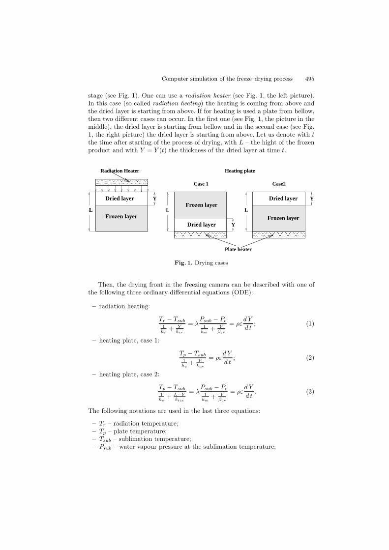
stage (see Fig. 1). One can use a radiation heater (see Fig. 1, the left picture).In this case (so called radiation heating) the heating is coming from above andthe dried layer is starting from above. If for heating is used a plate from bellow,then two different cases can occur. In the first one (see Fig. 1, the picture in themiddle), the dried layer is starting from bellow and in the second case (see Fig.1, the right picture) the dried layer is starting from above. Let us denote with t

the time after starting of the process of drying, with L – the hight of the frozenproduct and with Y = Y (t) the thickness of the dried layer at time t.

Radiation Heater

Plate heater

Heating plate

Case 1 Case2

LL L L

Y

Y

YFrozen layer

Frozen layerFrozen layer

Dried layer

Dried layer

Dried layer

Fig. 1. Drying cases

Then, the drying front in the freezing camera can be described with one ofthe following three ordinary differential equations (ODE):

– radiation heating:

Tr − Tsub

1hr

+ Ykcr

= λPsub − Pc

1km

+ Yβcr

= ρεd Y

d t; (1)

– heating plate, case 1:

Tp − Tsub

1hc

+ Ykcr

= ρεd Y

d t; (2)

– heating plate, case 2:

Tp − Tsub

1hc

+ L−Ykice

= λPsub − Pc

1km

+ Yβcr

= ρεd Y

d t. (3)

The following notations are used in the last three equations:

– Tr – radiation temperature;– Tp – plate temperature;– Tsub – sublimation temperature;– Psub – water vapour pressure at the sublimation temperature;

496 K. Georgiev et al.

– Pc – water vapour pressure at the condensation temperature;– hr – radiation heat transfer coefficient;– hc – contact heat transfer coefficient;– kcr – thermal conductivity of the dried layer;– kice – thermal conductivity of the frozen layer;– ρ – density coefficient;– ε – moisture content;– λ – latent of sublimation of the ice;– βcr – permeability of the dried layer;– km – external mass transfer coefficient.

2.2 Modelling the process of heat and mass transfer

The process of heat and mass transfer in the adsorbent camera is described bythe nonlinear partial differential equation (PDE) of parabolic type:

cρ∂T

∂t= LT + f(x, t, T ), x ∈ Ω, t > 0, (4)

where

LT =

d∑

i=1

∂

∂xi

(

k(x, t)∂T

∂xi

)

. (5)

The following notations are used in (4) and (5):

– T (x, t) – unknown distribution of the temperature;– d – dimension of the space (d = 2 in this study);– Ω ∈ Rd – computational domain (see Fig. 3);– k = k(x, t) > 0 – heat conductivity;– c = c(x, t) > 0 – heat capacity;– ρ > 0 – material density;– f(x, t, T ) – right-hand side function, which is responsible for the non–linear

process of transfer of water molecules in the adsorption container. This func-tion couples the two systems of equation (one of (1), (2) or (3), and (4)).

Let us mention, that the adsorbent camera consists of several subparts, and eachof them has their own conductivity, capacity and density coefficients.

Initial (6) and boundary (7) conditions are assigned to the parabolic equation(4):

T (x, 0) = T0(x), x ∈ Ω, (6)

T (x, t) = µ(x, t), x ∈ Γ ≡ ∂Ω, t > 0, (7)

where T0(x) is the initial distribution of the temperature in the computationaldomain and µ(x, t) is most often the surrounding of the freeze-drying devicetemperature.

Computer simulation of the freeze–drying process 497

3 Numerical treatment

3.1 Numerical treatment of the drying front equation

Let us write the three cases in describing the drying front in the freezing camerapresented by (1), (2) or (3) in the form:

dY

dt= f(t, Y ), t ∈ [0, T ], (8)

where the right–had–side function f is one of the left–side–functions in (1), (2) or(3) depending on the case of drying, dividing by ρ ε λ. An uniform discretizationof the time interval ti = t0 + iτ , where τ is the time–step, is used. For thenumerical solution of (8) the Runge–Kutta method of order fourth is applied([6]). Then

Yn+1 = Yn +

4∑

r=1

pj kj , (9)

where kj = τf(

tn + αjτ, Yn +∑j−1

l=1 βj,l kl

)

, j = 1, 2, 3, 4, and the parame-

ters in the last formulas are taken according to the so–called 3/8-Rule as follows:

p1 = p4 =1

8, p2 = p3 =

3

8, α1 = 0, α2 =

1

3α3 =

2

3α4 = 1,

β2,1 =1

3, β3,1 = −

1

3, β3,2 = β4,1 = β4,3 = 1, β4,2 = −1.

3.2 Numerical treatment of the heat and mass transfer front

equation

For the numerical solution of the above discussed boundary value problem theFinite Element Method (FEM) in space is used ([2]). In fact, the Courant linearfinite elements are chosen in this study. After the space discretization, the timederivatives are discretized via finite differences and well known Crank–Nicolsonscheme is used ([7]). The computational domain is discretaised via triangle finiteelements (see e.g. Fig. 4) using the computer mesh generator Triangle ([3, 9]).Options which are used for the mesh generating (generation of the main grid)are: minimal angle of a triangle (the most often used value is 30) and maximalarea of a single triangle (different for the different subdomains and dependingof the geometry). During the single run this basic grid can be refined dependingon a run parameter with a factor of k = 1, 2, 3, . . . and one can get respectivelyfrom each basic triangle 4, 16, 64, . . . finner triangle elements, after bisection ofthe basic grid triangles sides.

Let us denote with K and M the stiffness and mass matrices coming fromthe Finite Element approach. In our case they can be written in the forms:

498 K. Georgiev et al.

K = [Kij ]Ni,j=1 =

[∫

Ω

k∇Φi · ∇Φj dx

]N

i,j=1

,

M = [Mij ]Ni,j=1 =

[∫

Ω

cρ ΦiΦj dx

]N

i,j=1

.

Then, the parabolic equation (4) can be written in matrix form as:

MdT

dt+ KT = F , (10)

where

F =

[∫

Ω

f(x, t, T )Φj dx

]N

j=1

If we denote with τ the time step, with T n+1 the solution (temperature) on thecurrent time level and with T n the solution on the previous time level, and do anapproximation of the time derivative in (10) we will obtain the following systemof linear algebraic equations for the nodal values of T n+1:

(

M +Kτ

2

)

T n+1 =

(

M −Kτ

2

)

T n + τFn+1 + Fn

2. (11)

The Preconditioned Conjugate Gradient (PCG) method with a Modified In-complete Cholesky(MIC(0)) Preconditioner ([1, 5]) is used to solve the system of algebraic equations(11).

3.3 Structure of the computer model

The computer code realizing the above presented algorithm consists of two mainmodules according to the splitting done. The structure of the code is as follows:

– Numerical solution of the drying front equations in drying freeze camera(Runge–Kutta methods for solution of nonlinear ODE);

– Numerical solution of the heat–mass transfer equation in adsorbent camera(Crank–Nikolson method and FEM for parabolic PDEs):• triangulation of the computational domain (computer mesh generator

Triangle);• generation of the element stiffness and mass matrices and vectors;• assembling of the global stiffness and mass matrices and vectors;• solution of the systems of linear algebraic equations (PCG method with

MIC(0) preconditioner);• visualization of the output results.

The program modules are developed using the algorithmic languages Fortranand C++ under Linux/Unix operating system.

Computer simulation of the freeze–drying process 499

4 Numerical test on a real–life experiment

Many numerical experiments with known exact solutions were run in order to fixthe mesh and time parameters of the computer model. For the final test of thenumerical algorithm discussed above, an operating experimental unit was used(see Fig. 2). In this experiment the case where for the heating is used a platefrom bellow and the dried layer is started from bellow is used (see Fig. 1, casein the middle of the picture). The product which is subject to drying is put inthe left container. In the case study this container is a glass flask and the dryingproduct is grated carrots (see Fig. 2a)). The right container is the absorptioncamera (in this study it is again made from glass), where the zeolite granulesare placed (see Fig.2b)).

b)a)

vacuum

Fig. 2. The experiment

Two input parameters (data) for the solution of the heat–mass transfer equa-tion in the adsorbent container are obtained as output results from solution ofthe drying front movement equation:

– quantity of the sublimated water molecules per a time unit, and– the total time to finalize the process, i.e. the time interval for the parabolic

PDE [0, T ].

The quantity of the sublimated water molecules for a time unit is multiplied bythe adsorption heat coefficient in order to obtain the integral intensity of theheater.

We study the heat–mass transfer in the absorption camera via solving theabove introduced parabolic boundary value problem. The computational domain(see Fig. 3) is discretaised via triangle finite elements (see Fig. 4) using the com-puter mesh generator Triangle ([3, 9]). Let us mention that there are big jumpsin the values of the coefficients of the parabolic equation. The computational

500 K. Georgiev et al.

0

1

2

3

Fig. 3. The computational domain in the case–study (0 – glass, 1 – zeolite granules, 2– vacuum, 3 – air)

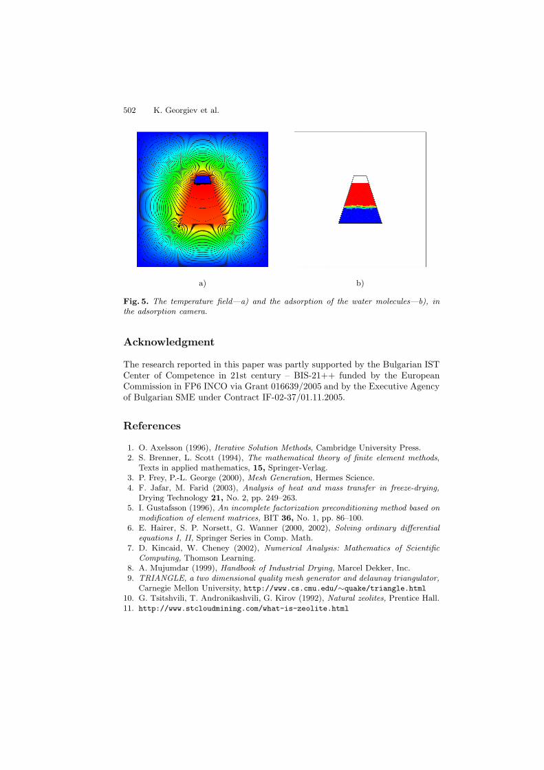
domain consists of four strongly different according to their physical character-istics, subdomains: glass, zeolite granules, vacuum and air. In the beginning ofthe process the air around the container with zeolite granules is with a roomtemperature (e.g. about 20C). A number of computer experiments were donein order to obtain appropriate values of the mesh parameters and the time step.The scalability of the code were studied (see bellow some results showing thegood scalability on several successive grids). Results from one of the providedcomputer test experiments, where a mesh with 6577 triangles and 3365 nodesand a time step τ = 10sec. were used are presented in this paper. The time toend the process of drying T is an input parameter. CPU time for running thecode on Pentium IV, 1.5 GHz is 393.82sec. The temperature field obtained inthe adsorption camera can be seen on Fig. 5, a), while on Fig. 5, b) one cansee how the zeolite granules are filled in with water molecules coming from thedrying container.

5 Conclusion

This paper is devoted to a numerical study of a freeze–drying process. Resultsfrom some of the performed numerical experiments are presented. In particular,the following subtasks are studied: (i) the drying front movement in the freezedryer, (ii) the temperature fields in the absorbent camera and (iii) the transferof the sublimated water molecules and their retention in the sorbent granules.Zeolites granules are used to sublimate the water molecules.

The mathematical model of the process of freeze–drying is described by asystem of time–depending differential equations.

Computer simulation of the freeze–drying process 501

Fig. 4. Finite element discretization of the computational domain

For implementation of the presented mathematical algorithm a computercode is developed using the algorithmic languages Fortran and C++. The scala-bility of the code was studied on three successive grids and the results are givenin Table 1.

Table 1. Scalability of the code

Number of CPU Ratio Ratiounknowns time nodes CPU time

N1 = 1174 T1 = 137.14 N2/N1 = 1.85 T2/T1 = 1.91

N2 = 2171 T2 = 261.52 N3/N2 = 1.55 T3/T2 = 1.51

N3 = 3365 T3 = 393.82 N3/N1 = 2.866 T3/T1 = 2.872

The output results of the numerical tests performed with the computer coderealizing the presented algorithm are compared with measurements coming froma real–life experiment. These comparisons show that the solver could be success-fuly used for simulation of the process of freezy–drying.

502 K. Georgiev et al.

a) b)

Fig. 5. The temperature field—a) and the adsorption of the water molecules—b), inthe adsorption camera.

Acknowledgment

The research reported in this paper was partly supported by the Bulgarian ISTCenter of Competence in 21st century – BIS-21++ funded by the EuropeanCommission in FP6 INCO via Grant 016639/2005 and by the Executive Agencyof Bulgarian SME under Contract IF-02-37/01.11.2005.

References

1. O. Axelsson (1996), Iterative Solution Methods, Cambridge University Press.2. S. Brenner, L. Scott (1994), The mathematical theory of finite element methods,

Texts in applied mathematics, 15, Springer-Verlag.3. P. Frey, P.-L. George (2000), Mesh Generation, Hermes Science.4. F. Jafar, M. Farid (2003), Analysis of heat and mass transfer in freeze-drying,

Drying Technology 21, No. 2, pp. 249–263.5. I. Gustafsson (1996), An incomplete factorization preconditioning method based on

modification of element matrices, BIT 36, No. 1, pp. 86–100.6. E. Hairer, S. P. Norsett, G. Wanner (2000, 2002), Solving ordinary differential

equations I, II, Springer Series in Comp. Math.7. D. Kincaid, W. Cheney (2002), Numerical Analysis: Mathematics of Scientific

Computing, Thomson Learning.8. A. Mujumdar (1999), Handbook of Industrial Drying, Marcel Dekker, Inc.9. TRIANGLE, a two dimensional quality mesh generator and delaunay triangulator,

Carnegie Mellon University, http://www.cs.cmu.edu/∼quake/triangle.html

10. G. Tsitshvili, T. Andronikashvili, G. Kirov (1992), Natural zeolites, Prentice Hall.11. http://www.stcloudmining.com/what-is-zeolite.html