ON THE CONVERGENCE OF THE KRIGING-BASED FINITE ELEMENT...

Submitted to International Journal of Computational Methods

1

ON THE CONVERGENCE OF THE KRIGING-BASED FINITE ELEMENT METHOD

F.T. WONG*

School of Engineering and Technology, Asian Institute of Technology Pathumthani, 12120, Thailand

[email protected]

W. KANOK-NUKULCHAI†

School of Engineering and Technology, Asian Institute of Technology Pathumthani, 12120, Thailand

[email protected] http://www.sce.ait.ac.th/people/faculty/kanok-nukulchai.asp

An enhancement of the FEM using Kriging interpolation (K-FEM) was recently proposed. This method offers advantages over the conventional FEM and mesh-free methods. With Kriging interpolation, the approximated field over an element is influenced not only by its own element nodes, but also by a set of satellite nodes outside the element. This results in incompatibility along inter-element boundaries. Consequently, the convergence of the solutions is questionable. In this paper, the convergence was investigated through a number of numerical tests. It is found that the solutions of the K-FEM with appropriate range of parameters converge to the corresponding exact solutions.

Keywords: finite element; Kriging; convergence.

1. Introduction

In the past two decades various mesh-free methods have been developed and applied to solve problems in continuum mechanics [e.g., see Liu (2003); Gu (2005)]. These methods have drawn attentions of many researchers partly due to their flexibility in customizing the approximation function for a desired accuracy. Of all the mesh-free methods, the methods using the Galerkin weak form such as the element-free Galerkin method (EFGM) [Belytschko et al. (1994)] and point interpolation methods [Liu (2003), pp. 250–300] maintain the same basic formulation as the FEM. However, although the EFGM and its variants have appeared in many academic articles for more than a decade, their applications seem to find little acceptance in real practice. This is in part due to the inconvenience in their implementation, such as the difficulties in constructing mesh-free approximations for highly irregular problem domains and in handling problems of material discontinuity [Liu (2003), pp. 15 and 644].

* Doctoral candidate † Professor of Structural Engineering

F.T. Wong and W. Kanok-Nukulchai 2

A very convenient implementation of EFGM was recently proposed [Plengkhom and Kanok-Nukulchai (2005)]. Following the work of Gu [2003], Kriging interpolation (KI) was used as the trial function. Since KI passes through the nodes and thus posses the Kronecker delta property, special treatment of boundary conditions is not necessary. For evaluating the integrals in the Galerkin weak form, finite elements could conveniently be used as the integration cells. The KI was constructed for each element by the use of a set of nodes in a domain of influence (DOI) composed of several layers of elements. Thus, for 2D problems, the DOI is in the form of a polygon. With this way of implementation, the EGFM of Plengkhom and Kanok-Nukulchai [2005] can be viewed as FEM with Kriging shape functions. This method is referred to as Kriging-based FEM (K-FEM) in this paper.

The K-FEM retains the advantages of mesh-free methods as follows: (1) Any requirement for high order shape functions can be easily fulfilled without any

change to the element structure. (2) The field variables and their derivatives can be obtained with remarkable accuracy

and global smoothness. A distinctive advantage of the K-FEM over other mesh-free methods is that it inherits the computational procedure of FEM so that existing general-purpose FE programs can be easily extended to include this new concept. Thus, the K-FEM has a higher change to be accepted in practice. The current trend in research in the K-FEM is towards extension and application of this new technique to different problems in engineering, such as applications to Reissner-Mindlin (RM) plates (Wong and Kanok-Nukulchai, 2006a; 2006b), problems with material discontinuity [Sommanawat and Kanok-Nukulchai (2006)], and adaptive procedure [Mazood and Kanok-Nukulchai (2006)].

Dai et al. [2003] pointed out that the method using standard Galerkin weak form with KI is nonconforming (incompatible) and so is the K-FEM. The very important issue of incompatibility and its effect on the convergence of the K-FEM have not been addressed in the previous researches. In this paper we addressed the incompatibility in the K-FEM—the reason why the K-FEM is not conforming was explained. The convergence was scrutinized through a number of numerical tests in plane-stress and RM plate problems. First, the weak patch tests for each problem were performed. Then, benchmark problems for plane-stress solids and for RM plates were solved. Relative error norms of displacement and strain energy were utilized to study the convergence. The convergence characteristics of the K-FEM with Gaussian and quartic-spline (QS) correlation functions were assessed and compared.

The present paper is organized as follows. Section 2 briefly reviews the formulation of KI. Its implementation in plane-stress/plane-strain and RM plate problems are presented in Section 3. In Section 4, the incompatibility in the K-FEM is discussed. Numerical studies on the convergence of the K-FEM are presented in Section 5 with concluding remarks in Section 6.

On the Convergence of the Kriging-based FEM

3

2. Kriging Interpolation

This section presents a review of the KI formulation in the context of K-FEM. A detail explanation and derivation of Kriging may be found in geostatistics literatures [e.g., Olea (1999); Wackernagel (1998)].

2.1. Formulation

Consider a continuous field variable u(x) defined in a domain Ω. The domain is represented by a set of properly scattered nodes xi, i=1, 2, …, N, where N is the total number of nodes in the whole domain. Given N field values u(x1), …, u(xN), the problem is to obtain an estimate value of u at a point 0 ∈Ωx .

The Kriging estimated value uh(x0) is a linear combination of u(x1), …, u(xn) in the form:

h0 1

( ) ( )n

i iiu uλ

== ∑x x (1)

where λi’s are termed as (Kriging) weights and n is the number of nodes surrounding point x0 inside a sub-domain 0Ω ⊆ Ωx . This sub-domain is referred to as domain of influence (DOI) in this paper. Considering the value of each function u(x1), …, u(xn) as the realizations of random variables U(x1), …, U(xn), Eq. (1) can be written as

h0 1

( ) ( )n

i iiU Uλ

== ∑x x (2)

The Kriging weights are determined by requiring the estimator Uh(x0) is unbiased, i.e.

h0 0E ( ) ( ) 0U U− =⎡ ⎤⎣ ⎦x x (3)

and by minimizing the variance of estimation error, h0 0var ( ) ( )U U−⎡ ⎤⎣ ⎦x x . Using the

method of Lagrange for constraint optimization problems, the requirements of minimum variance and unbiased estimator lead to the following Kriging equation system:

0( )+ =Rλ Pµ r x

T

0( )=P λ p x (4)

in which

11 1

1

( ) ... ( )

... ... ...

( ) ... ( )

n

n nn

C C

C C

=

⎡ ⎤⎢ ⎥⎢ ⎥⎢ ⎥⎣ ⎦

h h

R

h h

; 1 1 1

1

( ) ... ( )

... ... ...

( ) ... ( )

m

n m n

p p

p p

=

⎡ ⎤⎢ ⎥⎢ ⎥⎢ ⎥⎣ ⎦

x x

P

x x

(5)

[ ]T1 ... nλ λ=λ ; [ ]T

1 ... mµ µ=µ (6)

[ ]T0 10 20 0( ) ( ) ( ) ... ( )nC C C=r x h h h ; [ ]T

0 1 0 0( ) ( ) ... ( )mp p=p x x x (7)

R is an n n× matrix of covariances, C(hij), between two nodal values of U(x) evaluated at xi, xj; P is n m× matrix of polynomial values at the nodes; λ is 1n× vector of


Kriging weights; µ is 1m× vector of Lagrange multipliers; r(x0) is 1n× vector of covariance between the nodes and the node of interest, x0; and p(x0) is 1m× vector of polynomial basis at x0. In Eqs. (5) and (7),

[ ]( ) cov ( ), ( )i j i jC U U=h x x (8)

Solving the Kriging system, Eq. (4), results in Kriging weights as follows:

T T T0 0( ) ( )= +λ p x A r x B (9)

where

T 1 1 T 1( )− − −=A P R P P R ; 1 ( )−= −B R I PA (10)

Here, A is an m n× matrix; B is an n n× matrix; I is the n n× identity matrix. The expression for the estimated value uh given by Eq. (1) can be rewritten in matrix

form as

h T0( )u =x λ d (11)

in which [ ]T1( ) ... ( )nu u=d x x is 1n× vector of nodal values. Since the point x0 is

an arbitrary point in the DOI, the symbol x0 will henceforth be replaced by symbol x. Thus, using the usual finite element terminology, Eq. (11) can be expressed as

h1

( ) ( ) ( )n

i iiu N x u

== = ∑x N x d (12)

in which N(x)= λT(x) is the matrix of shape functions. Two key properties of Kriging shape functions that make them appropriate to be used

in the FEM are Kronecker delta (or interpolation) property and consistency property [Gu (2003); Plengkhom and Kanok-Nukulchai (2005)]. Due to the former property KI function passes through all nodal values. The consequence of the latter property is that if the basis includes all constants and linear terms, the Kriging shape functions will be able to reproduce a linear polynomial exactly.

2.2. Polynomial Basis and Correlation Function

Constructing Kriging shape functions in Eq. (12) requires a polynomial basis function and a model of covariance function. For the basis function, besides complete polynomial bases, it is also possible to use incomplete polynomial bases such as bi-linear, bi-quadratic and bi-cubic bases for interpolation in a 2D domain (for comparison, see Noguchi et al. [2000] for polynomial bases in the context of the moving least-square approximation).

Covariance between a pair of random variables U(x) and U(x+h) can be expressed in terms of correlation coefficient function or shortly, correlation function, as follows:

2( ) ( ) /Cρ σ=h h (13)

where ρ(h) is the correlation function, [ ]2 var ( )Uσ = x , and h is a vector separating two points, x and x+h. According to Gu [2003], σ2 has no effect on the final results and so in this study it is taken as 1. One of the widely used correlation model in the area of


5

computational mechanics is the Gaussian correlation function [e.g. Gu (2003), Dai et al. (2003), Wong and Kanok-Nukulchai (2006a)], viz.

2( ) ( ) exp( ( ) )h

hd

ρ ρ θ= = −h (14)

where θ>0 is the correlation parameter, h = h , i.e. the Euclidean distance between points x and x+h, and d is a scale factor to normalize the distance. In this study, d is taken to be the maximum distance between any pair of nodes in the DOI. Besides the Gaussian, we recently introduced the quartic spline (QS) correlation function (Wong and Kanok-Nukulchai, 2006a; 2006b) as follows:

2 3 41 6( ) 8( ) 3( ) for 0 1 ( )

0 for 1

h h h h

d d d dhh

d

θ θ θ θρ

θ

− + − ≤ ≤

=

>

⎧⎪⎪⎨⎪⎪⎩

(15)

Our study shows that using the quartic spline correlation function, Kriging shape functions are not sensitive to the change in parameter θ.

The proper choice of parameter θ is very important because it affects the quality of KI. In order to obtain reasonable results in the K-FEM, Plengkhom and Kanok-Nukulchai [2005] suggested a rule of thumb for choosing θ, namely θ should be selected so that it satisfies the lower bound,

101

1 1 10n a

iiN − +

=− ≤ ×∑ (16)

where a is the order of basis function, and also satisfies the upper bound,

det( ) 1 10 b−≤ ×R (17)

where b is the dimension of problem. For 2D problem with cubic basis function, for example, a=3 and b=2.

Numerical investigations on the upper and lower bound values of θ [Wong and Kanok-Nukulchai (2006a)] revealed that the parameter bounds vary with respect to the number of nodes in the DOI. Based on the results of the search for the lower and upper bound values of θ satisfying Eqs. (16) and (17), we proposed the following explicit parameter functions for practical implementation of the K-FEM for problems with 2D domains.

For the Gaussian correlation parameter, the parameter function is

low up(1 )f fθ θ θ= − + , 0 0.8f≤ ≤ (18)

where f is a scale factor, θlow and θup are the lower and upper bound functions as follows:

low 2

0.08286 0.2386 for 3 10

-8.364E - 4 0.1204 0.5283 for 10 55

0.02840 2.002 for 55

n n

n n n

n n

θ

− ≤ <

= + − ≤ ≤

+ >

⎧⎪⎨⎪⎩

(19)


up 2

0.34 0.7 for 3 10

-2.484E-3 +0.3275 0.2771 for 10 55

0.05426 7.237 for 55

n n

n n n

n n

θ

− ≤ <

= − ≤ ≤

+ >

⎧⎪⎨⎪⎩

(20)

For the QS correlation parameter, the parameter function is

0.1329 0.3290 for 3 10

1 for 10

n n

nθ

− ≤ <=

≥

⎧⎨⎩

(21)

2.3. Layered-Element Domain of Influence

Let us consider a 2D domain mesh using triangular elements, as illustrated in Fig. 1. For each element, KI is constructed based upon a set of nodes in a polygonal DOI encompassing a predetermined number of layers of elements. The KI function over the element is given by Eq. (12). By combining the KI of all elements in the domain, the global field variable is approximated by piecewise KI. This way of approximation is very similar with the approximation in the conventional FEM.

It should be mentioned here that it is also possible to use quadrilateral elements to implement the concept of layered-element DOI. Mesh with triangular elements is chosen in this study owing to its flexibility in representing complex geometry and its ease to be automatically generated.

The number of layers for each element must cover a number of nodes in such a way that the Kriging equation system, Eq. (4), is solvable. If an m-order polynomial basis is employed, the DOI is required to cover a number of nodes, n, that is equal or greater than the number of terms in the basis function, i.e. n m≥ . Based on our experience, the minimum number of layers for different polynomial bases is listed in Table 1. As the number of layers increases, the computational cost is higher. Thus we recommend the use of minimum number of layers for each polynomial basis.

Fig. 1. Domain of influence for element el with one, two and three layers of elements [Plengkhom and Kanok-Nukulchai (2005)].


7

Table 1. Minimum number of layers for various basis functions.

Basis Minimum number of layers

Linear 1 Quadratic, Bi-linear 2 Cubic, Bi-quadratic 3 Quartic, Bi-cubic 4

3. Formulation

3.1. K-FEM for Plane-Strain/Plane-Stress Solids

The governing equations for plane-strain/plane-stress problems in Cartesian coordinate system can be written in a weak form as follows:

T T T

V V SdV dV dSδ δ δ= +∫ ∫ ∫ε σ u b u t (22)

where Tu v=u is the displacement vector; T

x y xyε ε γ=ε is the vector of

2D strain components; T

x y xyσ σ τ=σ is the vector of 2D stress components;

T

x yb b=b is the body force vector; T

x yt t=t is the surface traction force

vector; V is the 3D domain occupied by the solid body; and S is the surface on which the traction t is applied.

Suppose the domain V is subdivided by a mesh of Nel elements and N nodes. To obtain an approximate solution using the concept of KI with layered-element DOI, for each element e=1, 2, …, Nel the displacement components u and v are approximated by the KI as follows:

1

( , ) ( , )n

i iiu x y N x y u

=∑ ; 1

( , ) ( , )n

i iiv x y N x y v

=∑ (23)

Here, Ni(x,y) denotes Kriging shape function associated with node i; ui and vi are nodal displacement components in the x and y directions, respectively; n is the number of nodes in the DOI of an element, which generally varies from element to element. Employing the standard formulation procedure of the FEM [e.g., see Cook (2002) et al., pp. 88–89; Zienkiewicz and Taylor (2000), pp. 19–26], we may obtain the equilibrium equation for each element as follows:

e e e=k d f (24) where the element stiffness matrix ( 2 2n n× )

Te e eeV

dV= ∫k B EB (25)

the displacement vector ( 2 1n× )

T1 1 2 2

en nu v u v u v=d (26)

and the consistent nodal force vector of element e ( 2 1n× )


T Te e e e ee eV S

dV dS= +∫ ∫f N b N t (27)

Matrix Ne is the Kriging shape function matrix, i.e.

1 2

1 2

0 0 0

0 0 0ne

n

N N N

N N N=⎡ ⎤⎢ ⎥⎣ ⎦

N (28)

Be is the element strain-displacement matrix, i.e.

1, 2, ,

1, 2, ,

1, 1, 2, 2, , ,

0 0 0

0 0 0x x n x

ey y n y

y x y x n y n x

N N N

N N N

N N N N N N

=

⎡ ⎤⎢ ⎥⎢ ⎥⎢ ⎥⎣ ⎦

B (29)

and E is the constitutive matrix, which, for the case of isotropic material, can be expressed in terms of modulus elasticity E and Poisson’s ratio ν as follows:

2

1 0

1 01

0 0 (1 ) / 2

Eν

νν

ν

=−

−

⎡ ⎤⎢ ⎥⎢ ⎥⎢ ⎥⎣ ⎦

E (30)

with

21

EE E

ν

=

−

⎧⎪⎨⎪⎩

and

1

νν ν

ν

=

−

⎧⎪⎨⎪⎩

for plane stress

for plane strain (31)

Ve is the 3D domain of element e and Se is the surface of element e on which the traction t is applied.

For a triangular element of the thickness h and the area Ae, with traction force on edge se, Eqs. (25) and (27) can be expanded as follows:

Te e eeA

h= ∫k B EB (32)

T Te e e e ee eA s

h dA h ds= +∫ ∫f N b N t (33)

3.2. K-FEM for Reissner-Mindlin Plates

Consider a plate of uniform thickness, h, homogeneous, referred to a three-dimensional Cartesian coordinate system with the x-y plane lying on the middle surface of the plate (Fig. 2). Its domain, V, is defined as

[ ] 3 2( , , ) | / 2 , / 2 , ( , )V x y z z h h x y S= ∈ ∈ − ∈ ⊂ (34)


9

Rotation of a normal line has two components, namely ψx and ψy. The positive sign convention for these rotation components and displacement components is showed in Fig. 2. For small displacement and rotation, the displacement field is described by

3D

( , )

( , )

( , )

x

y

u z x y

v z x y

w w x y

ψ

ψ

−

= = −

⎧ ⎫ ⎧ ⎫⎪ ⎪ ⎪ ⎪⎨ ⎬ ⎨ ⎬⎪ ⎪ ⎪ ⎪⎩ ⎭ ⎩ ⎭

u (35)

where w(x,y) is the deflection of a point initially lying on the reference plane, S, and ψx(x,y) and ψy(x,y) are the normal line rotation components around its midpoint with respect to the –y and x directions, respectively.

The governing equations for static deflection of RM plates under transversal load q(x,y) can be written in a weak form as follows:

T T Tb s s sS S S

dS dS dSδ δ δ+ =∫ ∫ ∫κ D κ ε D ε u p (36)

In this equation,

T

, , , ,x x y y x y y xψ ψ ψ ψ= +κ (37)

is the curvature vector,

T

s x z y zγ γ=ε (38)

is the transverse-shear vector,

T

x yw ψ ψ=u (39)

is the vector of three independent field variables for RM plates,

T0 0q=p (40)

is the surface force vector,

Fig. 2. Positive directions for displacement and rotation components.


3

b 2

1 0

1 012(1 )

0 0 (1 ) / 2

Ehν

νν

ν

=−

−

⎡ ⎤⎢ ⎥⎢ ⎥⎢ ⎥⎣ ⎦

D (41)

is the elasticity matrix for bending deformation and

s

1 0

0 1Gkh=

⎡ ⎤⎢ ⎥⎣ ⎦

D (42)

is the elasticity matrix for transverse-shear deformation. Here,

2(1 )

EG

ν=

+ (43)

is the shear modulus and k is a shear correction factor to account for the parabolic z-direction variation of transverse shear stress. The accepted value of k for a homogeneous plate is k=5/6 [Cook et al. (2002), pp. 534–535].

Suppose the domain S is subdivided by a mesh of Nel triangular elements and N nodes. To obtain an approximate solution using the concept of KI with layered-element DOI, for each element e=1, 2, …, Nel the plate field variables are approximated by the KI as follows:

1

( , ) ( , )n

i iiw x y N x y w

=∑

1

( , ) ( , )n

x i x iix y x yψ η ψ

=∑ ; 1

( , ) ( , )n

y i y iix y x yψ ξ ψ

=∑ (44)

Here Ni(x,y), ηi(x,y) and ξi(x,y) denote Kriging shape functions associated with node i for approximating defection, rotation in y-direction, and rotation in x-direction, respectively; wi, ψx i and ψy i are nodal deflection, nodal rotation in the –y-direction, and nodal rotation in the x-direction, respectively. Shape functions Ni, ηi and ξi do not have to be the same; they are independent of each other. In this study, however, they are taken to be the same, i.e.

( , ) ( , ) ( , )i i ix y x y N x yη ξ= = (45)

Inserting Eq. (44) into the variational equation of RM plates, Eq. (36), leads to the following discretized equilibrium equation for each element:

e e e=k d f (46) in which the element stiffness matrix ( 3 3n n× ) is T T

b b b b s s se e e e e e e

e es S SdS dS= + = +∫ ∫k k k B D B B D B , (47)

the element nodal displacement vector ( 3 1n× ) is

T

1 1 1 2 2 2e

x y x y n x n y nw w wψ ψ ψ ψ ψ ψ=d (48)

and the element nodal force vector ( 3 1n× ) is


11

Te e eeS

dS= ∫f N p (49)

In Eqs. (47) and (49), matrices Ne, beB and s

eB are defined as follows:

1

1

1

0 0 0 0

0 0 0 0

0 0 0 0

ne

n

n

N N

N N

N N

=

⎡ ⎤⎢ ⎥⎢ ⎥⎢ ⎥⎣ ⎦

N (50)

1

b 1

1 1

0 0 0 0

0 0 0 0

0 0

, ,, ,

, , , ,

x n xe

y n y

y x n y n x

N N

N N

N N N N

=

⎡ ⎤⎢ ⎥⎢ ⎥⎢ ⎥⎣ ⎦

B (51)

1 1s

1 1

0 0

0 0

, ,, ,

x n x ne

y n y n

N N N N

N N N N

− −=

− −

⎡ ⎤⎢ ⎥⎣ ⎦

B (52)

3.3. Global Discretized Equilibrium Equation

The global discretized equilibrium equation, =KD F (53) can be obtained from the element equilibrium equation, i.e. Eq. (24) for plane-stress/plane-strain problems and Eq. (46) for RM plates, by using the assembly procedure, i.e.

el1

N ee== ΑK k ; el

1N ee== ΑD d ; el

1N ee== ΑF f (54)

Here K is the global stiffness matrix, D is the global nodal displacement vector, F is the global nodal force vector, and el

1Ne=Α denotes the assembly operator. It should be

mentioned here that the assembly process for each element involves all nodes in the element’s DOI, not only the nodes within the element as in the conventional FEM.

4. Incompatibility in the K-FEM

As described in Sec. 2, the KI is constructed for each element using a set of nodes, within and outside the element, in a predetermined layered-element DOI. Therefore, within each element the interpolation function is naturally continuous. However, along the element edges between two adjacent elements the function is not perfectly continuous because the KI for each of the two neighboring elements is constructed using different set of nodes.

For illustration, we consider element 1 and element 2 in a 2D domain as shown in Fig. 3 and suppose we use two element layers as the DOI for each element. Polygon A-B-C-D-E-F-G-H-I is the DOI for element 1 and polygon B-C-D-K-F-G-H-I-J is the DOI for element 2. The KI within element 1 is constructed using the 12 nodes in the first polygon while the KI within element 2 is constructed using the 11 nodes in the second polygon. As a result, the function along its edge LM of element 1 is different from the


function along the edge LM of element 2. In other words, the displacement function is not continuous across the common edge LM of the two neighboring elements. The foregoing explanation is principally the same as that presented by Dai et al. [2003] in the context of the EFGM with KI.

To illustrate further the inter-element incompatibility in the K-FEM, we consider again the domain shown in Fig. 3 and suppose now the value at node K is one and the other nodal values are zero. According to the KI of element 1, the function along the interface LM is zero function since the value at node K does not have any effect to the KI within element 1. On the contrary, according to element 2, the function along LM is not zero function because the shape function associated with node K is not zero between nodes L and M.

Thus it is apparent that the K-FEM does not satisfy the inter-element compatibility requirement (nonconforming), except for the K-FEM with linear basis and one layer DOI. Is this incompatibility acceptable? It is acceptable if it tends toward zero as the mesh is repeatedly refined [Cook et al. (2002), p. 7]. In other words, the inter-element compatibility needs only be satisfied in the limit as the size of the element tends to zero. This is assessed through the weak patch test and convergence studies in the following section.

It should be mentioned here that it is also possible to employ a constrained variational equation in the K-FEM to deal with the incompatibility [e.g. see Dai et al. (2003)]. This approach, however, will destroy the key advantage of the K-FEM mentioned in Sec 1., namely its ease to be implemented in a general-purpose finite element program. It is for this reason we do not resort to this approach to deal with the incompatibility.

5. Numerical Tests

In the following tests, the integrals over each triangular element in the expressions for element stiffness matrices, Eqs. (32) and (47), and for nodal force vectors, Eqs. (33) and (49), were computed using the 6-point quadrature rule for triangles [see e.g. Hughes (1987), p. 173]. This rule was elected because it may give reasonably accurate results yet inexpensive in terms of computational cost. For computing the line integral in Eq. (33),

Fig. 3. The domain of influences of element 1 and element 2.


13

the 2-point Gaussian quadrature for line integral was used since it can yield exact nodal force vector for edge traction force with cubic distribution or less.

Abbreviations in the form of P*-*-G* or P*-*-QS, in which the star denotes a number, were adopted in this section to designate various options of the K-FEM. The first syllable denotes polynomial basis with the order indicated by the number next to letter P. The middle star denotes number of layers. The last syllable denotes the Gaussian correlation function with the adaptive parameter given by Eq. (18) and with the scale factor f indicated by the number next to letter G (in percent); QS denotes the quartic spline correlation function with the adaptive parameter given by Eq. (21). For example, P3-3-G50 means cubic basis, 3 element-layers, Gaussian correlation function with mid-value parameter function, i.e. f=0.5.

5.1. Plane-Stress/Plane-Strain Solids

To study the convergence of the K-FEM for plane-stress/plane-strain solids, two measures of error were utilized. The fist one is relative L2 error norm of displacement, defined as

app exact T app exact

exact T exact

1 2( ) ( )

( )V

u

V

dVr

dV

− −=⎛ ⎞⎜ ⎟⎜ ⎟⎝ ⎠

∫∫

u u u u

u u (55)

where uapp and uexact are approximate and exact displacement vectors, respectively. The second one is relative error norm of strain energy, defined as

app exact T app exact

exact T exact

1 2( ) ( )

( )V

VdV

rdVε

− −=⎛ ⎞⎜ ⎟⎜ ⎟⎝ ⎠

∫∫

ε ε E ε ε

ε Eε (56)

where εapp and εexact are approximate and exact strain vectors, respectively. For computing these relative errors, the 13-point quadrature rule for triangles was employed for each element.

5.1.1. Weak Patch Test

Patch test is a test to a “patch” of finite elements with states of constant strains or constant stresses. Since the K-FEM is nonconforming, it will not pass the patch test for a patch with a large size of elements. Passing the patch test for a large size of elements, however, is not a necessary condition for convergence. The necessary and sufficient condition for convergence is to pass the patch test in the limit, as the size of the elements in the patch tends to zero [Zienkiewicz and Taylor (2000), p. 254; Razzaque (1986)], provided that the system of equations is solvable and all integrations are exact. This kind of test is referred to as weak patch test [Zienkiewicz and Taylor (2000), pp. 250–275, Cook et al. (2002), p. 240].

The patch used for the weak patch test is shown in Fig. 4(a). It was adopted from the patch proposed by MacNeal and Harder [1985]. In order to be consistent with


displacement field u=10–3(x+y/2), v=10–3(y+x/2), 30.24 10u −= × and 30.12 10v −= × were prescribed at node B. The initial course mesh, which includes 25 nodes, is shown in Fig.4(b). We defined the element characteristic size for this mesh hc=0.06. Subsequently, mesh refinements were performed by subdividing the elements.

The following K-FEM options were elected for the weak patch test: P2-2 with G0, G50, G80, QS and P3-3 with G0, G50, G80, QS. Displacement error norms of the K-FEM solutions were plotted against element characteristic sizes in Fig. 5. The average convergence rate (R) of each option was also shown in the legends. The figure shows that the K-FEM does not pass the test in any mesh but the solutions converge. For the K-FEM of option P3-3-G0, however, the convergence is doubtful. Therefore, we conclude that the K-FEM passes the weak patch test, except that with option P3-3-G0. For the K-FEM with Gaussian correlation functions, as the parameter θ comes closer to the upper bound values, the convergence rate and accuracy increase. The K-FEM with the QS is the best in term of convergence rate (R=1.45 for P2-2 and R=1.82 for P3-3).

The strain energy error norms vs. element characteristic sizes were shown in Fig. 6. These energy errors are mainly due to “gaps” or “overlaps” along the interface between two elements because the round-off and numerical integration errors are negligible.

(a)

(b) Fig. 4. (a) A patch under constant stresses and (b) its initial mesh for the weak patch test.


15

Therefore, in this case the energy error may serve as a measure of the degree of incompatibility of the K-FEM. The figure shows that the incompatibilities of the K-FEM with various options tend to decrease as the mesh was refined. The K-FEM with QS correlation function is “more compatible” than that with the Gaussian.

5.1.2. An Infinite Plane-Stress Plate with A Hole

An infinite plane-stress plate with a circular hole of radius a=1 is subjected to a uniform tension Tx=100 at infinity [Tongsuk and Kanok-Nukulchai (2004)] (Fig. 7(a)). In view of the symmetry, only the upper right quadrant of the plate, 0 5x≤ ≤ and 0 5y≤ ≤ , was analyzed. Zero normal displacements were prescribed on the symmetric boundaries and the exact traction boundary conditions were imposed on the right (x=5) and top (y=5) edges.

The initial course mesh of 42 nodes is shown in Fig. 7(b). The element characteristic size for this problem is taken as the distance between two nodes at the right or top edge, i.e. hc=1. Subsequently, the mesh was refined by subdividing the previous element into four smaller elements. The refined meshes considered in this test are meshes with hc = 0.5 (141 nodes) and hc = 0.25 (513 nodes). In performing the analysis with hc =0.25

(a) P2-2

(b) P3-3

Fig. 5. Relative error norm of displacement vs. element characteristic size for the patch analyzed using the K-FEM with: (a) P2-2, (b) P3-3. The number after the code for K-FEM option in the legend indicates the average convergence rate.


using Gaussian correlation function, the scale factor f=0.79 was used in place of f=0.8 because the use of f=0.8 resulted in det(R) exceeding the upper bound criterion, Eq. (17), for some elements.

The convergence characteristics for displacement and strain energy are shown in Figs. 8(a) and 8(b), respectively. The figures show that the rates of convergence of all K-FEM options are nearly equal, for displacement as well as strain energy. The fastest convergence rate in term of displacement error is achieved by the K-FEM with P3-3-G80 (the rate, R=2.60) while the fastest one in term of strain energy error is the K-FEM with P3-3-QS (R=1.37). Theoretically, the accuracy and convergence rate of the K-FEM with cubic basis are higher than those with quadratic basis. However, this is not the case because of the incompatibilities of the K-FEM.

5.2. Reissner-Mindlin Plates

The convergence of the K-FEM for RM plates was assessed in terms of the relative L2 error norm of displacement, viz.

(a) P2-2

(b) P3-3

Fig. 6. Relative error norm of strain energy vs. element characteristic size for the patch analyzed using the K-FEM with: (a) P2-2, (b) P3-3.


17

app exact3D 3D

exact3D

ur−

=u u

u (57)

where app3Du and exact

3Du are approximate and exact displacement vectors of 3D solid, respectively. The displacement norm in Eq. (57) was expanded as follows:

( ) ( )T 2 2 23D 3D 3D

1 2 1 2( )

V VdV u v w dV= = + +∫ ∫u u u (58)

Substituting u, v, and w in this equation with those stated in Eq. (35) and then integrating over the thickness resulted in

3

2 2 23D ( )

3 x yS S

hh w dS dSψ ψ= + +∫ ∫u (59)

(a)

(b) Fig. 7. (a) An infinite plate with a circular hole and (b) the initial mesh of the shaded area.


As in the previous tests, the 13-point quadrature rule for triangles was employed to evaluate the integrals in this equation for each element.

5.2.1. Weak Patch Tests

The same patch and meshes as in the previous patch test (Fig. 4) were used in the following tests, except the loading condition and the thickness. Two conditions of the patch were considered, namely (1) constant curvature and (2) constant transverse shear strain. The length-to-thickness ratio of the patch was differently specified for each condition of the tests. Based on the study on the performance of various K-FEM options in alleviating shear locking (Wong and Kanok-Nukulchai, 2006a; 2006b), the following K-FEM options were elected for the patch tests: P3-3-G0, P3-3-QS, P4-4-G0, and P4-4-QS.

Constant curvature condition The boundary of the patch was imposed by the essential boundary conditions as presented in MacNeal and Harder [1985], i.e.

3 2 210 ( ) / 2w x xy y−= + +

(a)

(b) Fig. 8. Relative error norms of: (a) displacement and of (b) strain energy and their convergence rates for the holed plate.


19

310 ( / 2)x w x x yψ −= ∂ ∂ = + ; 310 ( / 2 )y w y x yψ −= ∂ ∂ = + (60)

These fields lead to the following constant curvatures and moments:

T 31 1 1 10−= ×κ ; T 710 / 9 10 / 9 1/ 3 10−= − ×M (61)

Shear strains and shear stresses corresponding to these constant curvatures are zero. The length-to- thickness ratio of the patch was set to 240 (h=0.001) in order to represent thin plates.

Displacement error norms of the K-FEM solutions were plotted against element characteristic sizes in Fig. 9. It can be seen that from the second mesh (hc =0.03) until the last mesh (hc =0.0075) the solutions of the K-FEM converge, except for the K-FEM with option P3-3-G0. The solutions for the mesh of hc=0.06 (25 nodes) are exceptionally accurate because 16 of the 25 nodes are located at the boundary and accordingly imposed by the boundary conditions, Eq. (60). Thus, the nodal displacements associated with the 16 boundary nodes are automatically exact. In addition, for cases of relatively small number of nodes in a domain, the K-FEM may yield extraordinary accurate results because the KI is close to a polynomial function of higher order than the basis function. We conclude that the K-FEM with options P3-3-QS, P4-4-G0, and P4-4-QS pass the weak constant curvature patch test but the K-FEM with P3-3-G0 does not pass. The K-FEM with QS correlation function has better convergence characteristic than that with G0. This finding is similar to the one in the plane stress condition.

Constant transverse shear-strain condition A state of constant transverse shear strains and zero curvatures, i.e.

T 6s 1 1 10−= ×ε ; T0 0 0=κ (62)

can be obtained, with all equilibrium equations satisfied, only for the extreme case of thick plates [Batoz and Katili (1992)]. In this test, an extremely-thick plate with the

Fig. 9. Relative error norm of displacement vs. element characteristic size for the constant curvature patch test. The numbers in the legend indicate the average convergence rates from the second mesh up to the last.


length-to-thickness ratio 0.0024 (h=100) was considered. The displacement fields leading to the constant shear strains, Eq. (62), are as follows:

610 ( ) / 2w x y−= + ; 61/ 2 10xψ −= − × ; 61 / 2 10yψ −= − × (63)

The shear forces corresponding to the constant shear strains are

T100 / 3 100 / 3=Q (64)

The test was performed by imposing nodal values on the boundary according to the fields stated by Eq. (63). The error indicator used in this test is the relative L2 error norm of deflection, defined as

app exact 2

exact 2

1 2( )

( )S

w

S

w w dSr

w dS

−=⎛ ⎞⎜ ⎟⎜ ⎟⎝ ⎠

∫∫

(65)

This indicator was used here instead of the displacement error norm, Eq. (57), because the thickness of the plate is extremely large so that if we used the error norm of Eq. (57), the norm would be dominated by the rotation errors. We found that these rotation errors are relatively constant for different degrees of mesh refinements.

The plot of the relative deflection error norms for the K-FEM with different analysis options is shown in Fig. 10. It can be seen that all of the options lead to converging solutions and therefore they pass the weak constant shear patch test. As in the previous test, the accuracy and convergence rate of the K-FEM with QS is better than that with G0.

5.2.2. A Thin Square Plate

We considered a hard simply-supported square plate of the length L=100 and length-to-thickness ratio L/h=100 under uniform transverse load 61 10q −= − × . The modulus of elasticity is 62 10E = × and Poisson’s ratio is v=0.3. To study the convergence of the K-FEM solutions, a quadrant of the plate was discretized with different degrees of mesh refinement: 4 4× (hc=12.5, Fig. 11), 6 6× (hc=8.33), …,12 12× (hc=4.17). The meshes

Fig. 10. Relative error norm of deflection vs. element characteristic size for the constant shear patch test.


21

were automatically generated using Delaunay algorithm and thus the triangles have random orientation, such as shown in Fig 11. The K-FEMs with P3-3-QS and P4-4-QS were chosen in this and subsequent tests because they showed good performance both in the shear locking study (Wong and Kanok-Nukulchai, 2006a; 2006b) and patch tests. In computing the displacement error norms, Eq. (57), the exact displacement fields according to the thick plate theory [Reissman (1988), pp. 136–137] were used.

The displacement error norms were plotted against element characteristic sizes in Fig. 12. The figure shows excellent convergence characteristics. The results with the option of P4-4-QS, as expected, are more accurate than those with P3-3-QS. However, the best converge rate is achieved for P3-3-QS with R=5.54. The reason for this is that the incompatibilities in the K-FEM with P3-3-QS diminished faster than that in the K-FEM with P4-4-QS.

5.2.3. A Thick Circular Plate

A clamped circular plate of the diameter D=100 and length-to-thickness ratio D/h=5 was considered. The uniform load intensity and material properties are the same as in the

Fig. 11. Initial mesh of a quarter of the square plate (4-by-4).

Fig. 12. Relative error norms of displacement and their convergence rates for the square plate.


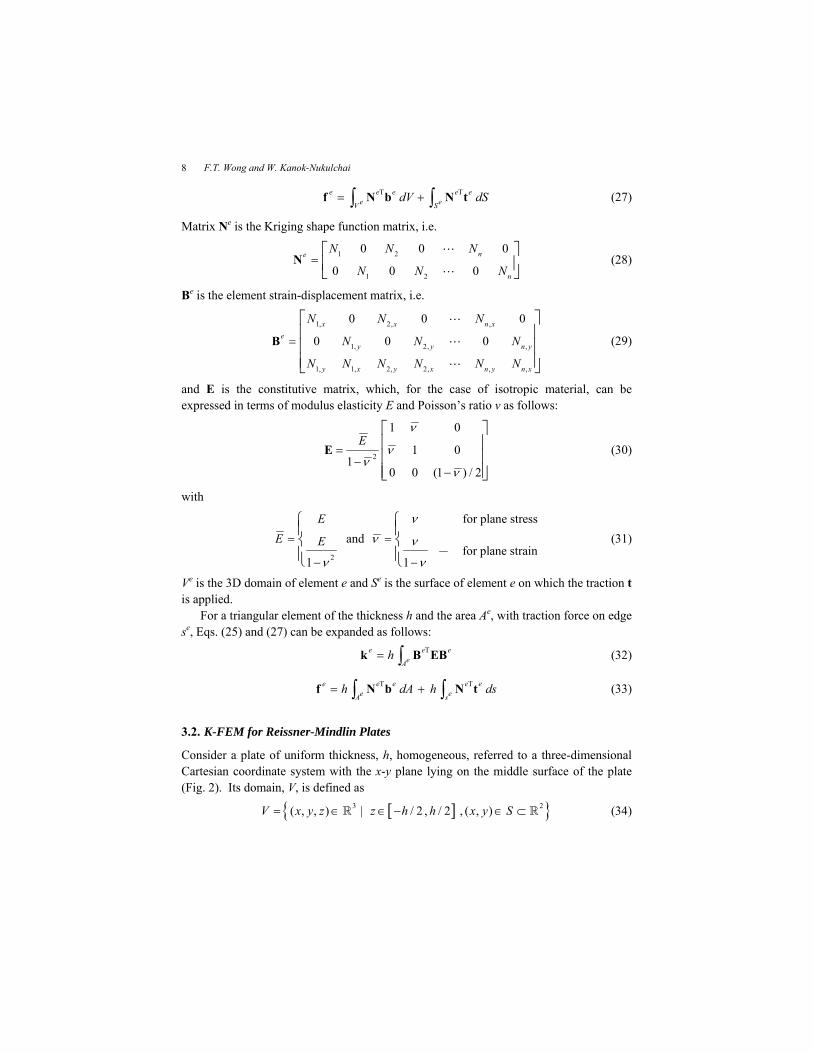
previous test (the thin square plate). A quadrant of the plate was discretized with different degrees of mesh refinement as shown in Fig. 13. The element characteristic size hc was defined as the length of the first line segment in the x-axis (which is one of the edges of the triangle in the center). In computing the displacement error norms, the exact solutions based on the thick plate theory [Reismann (1988), p. 142] were used.

The convergence of the solutions in terms of the displacement error norm is shown in Fig. 14. The figure shows that the average convergence rates for P3-3-QS and P4-4-QS are nearly equal. The solutions of P3-3-QS are slightly more accurate that those with P4-4-QS. This fact disagrees with the usual tendency in the standard FEM, namely the higher degree of shape functions, the more accurate results are gained. This disagreement occurs because in this problem the incompatibility in the K-FEM with P4-4-QS is more severe that that in the K-FEM with P3-3-QS.

6. Conclusions

Convergence characteristics of the K-FEM with different options have been studied in the context of plane stress and Reissner-Mindlin plate problems through a number of numerical tests. It is found that the K-FEM with different options passed the weak patch

(a) Mesh no. 1: 34 nodes, 47 elements, hc=10

(b) Mesh no. 2: 43 nodes, 62 elements, hc=8

(c) Mesh no. 3: 76 nodes, 119 elements, hc=5

(d) Mesh no. 4: 208 nodes, 359 elements, hc=2.2

Fig. 13. Meshes of a quarter of the circular plate (adopted from Kokaew [2003, p. 42]).


23

tests except the K-FEM with P3-3-G0. For the K-FEM with the Gaussian correlation function, the convergence characteristics were better as the correlation parameters were closer to the upper bound. The K-FEM with the QS correlation function had better convergence characteristics than that with the Gaussian as its solutions are not sensitive to the change of the correlation parameter. The numerical tests with several benchmark problems demonstrated reliable and good convergence characteristics of the K-FEM using QS correlation functions.

Passing the weak patch tests indicates that the incompatibility decreases as the mesh is refined. Therefore, the convergence of the K-FEM with appropriate options is guaranteed. The use of the QS correlation function in a K-FEM for analyses of two-dimensional problems is therefore recommended. It is also confirmed that the K-FEM is a viable alternative to the conventional FEM and has great potential in engineering applications.

References

Batoz, J. L. and Katili, I. (1992). On a simple triangular Reissner/Mindlin plate element based on incompatible modes and discrete constraints. Int. J. Num. Meth. Eng., 35: 1603–1632.

Belytschko, T., Lu, Y. Y. and Gu, L. (1994). Element-free Galerkin methods. Int. J. Num. Meth. Eng., 37: 229–256.

Cook, R. D., Malkus, D. S., Plesha, M. E. and Witt, R. J. (2002). Concepts and Applications of Finite Element Analysis, 4th edn. John Wiley and Sons, Madison.

Dai, K. Y., Liu, G. R., Lim, K. M. and Gu, Y. T. (2003). Comparison between the radial point interpolation and the Kriging interpolation used in meshfree methods. Comput. Mech., 32: 60–70.

Gu, L. (2003). Moving Kriging interpolation and element-free Galerkin method. Int. J. Num. Meth. Eng., 56: 1-11.

Gu, Y. T. (2005). Meshfree methods and their comparisons. Int. J. Comput. Meth., 2: 477–515. Hughes, T. J. R. (1987). The Finite Element Method: Linear Static and Dynamic Finite Element

Analysis. Prentice-Hall, New Jersey. Kokaew, N. (2003). Triangular plate bending element based on moving least square shape

functions. Master of Engineering Thesis, Asian Institute of Technology, Pathumthani. Liu, G. R. (2003). Mesh Free Methods. CRC Press, Boca Raton.

Fig. 14. Relative error norms of displacement and their convergence rates for the circular plate.


MacNeal, R. H. and Harder, R. L. (1985). A proposed standard set of problems to test finite element accuracy. Finite Elements in Analysis and Design, 1: 3–20.

Mazood, Z. and Kanok-Nukulchai, W. (2006). An adaptive mesh generation for Kriging element-free Galerkin method based on Delaunay triangulation, in Emerging Trends: Keynote Lectures and Symposia. Proc. 10th East-Asia Pacific Conf. Struct. Eng. Const., Bangkok, 3–5 Aug. 2006, pp. 499–508.

Noguchi, H., Kawashima, T. and Miyamura, T. (2000). Element free analyses of shell and spatial structures. Int. J. Num. Meth. Eng., 47: 1215–1240.

Olea, R. A. (1999). Geostatistics for Engineers and Earth Scientists. Kluwer Academic Publishers, Boston.

Plengkhom, K. and Kanok-Nukulchai, W. (2005). An enhancement of finite element methods with moving Kriging shape functions. Int. J. Comput. Meth., 2: 451–475.

Razzaque, A. (1986). The patch test for elements. Int. J. Num. Meth. Eng., 22: 63–71. Reissmann, H. (1988). Elastic Plates: Theory and Application. John Wiley and Sons, New York. Sommanawat, W. and Kanok-Nukulchai, W. (2006). The enrichment of material discontinuity in

moving Kriging methods, in Emerging Trends: Keynote Lectures and Symposia. Proc. 10th East-Asia Pacific Conf. Struct. Eng. Const., Bangkok, 3–5 Aug. 2006, pp. 525–530.

Tongsuk, P. and Kanok-Nukulchai, W. (2004). Further investigation of element-free Galerkin method using moving Kriging interpolation. Int. J. Comput. Meth., 1: 345–365.

Wackernagel, H. (1998). Multivariate Geostatistics, 2nd edn. Springer, Berlin. Wong, F. T. and Kanok-Nukulchai, W. (2006a). Kriging-based finite element method for analyses

of Reissner-Mindlin plates, in Emerging Trends: Keynote Lectures and Symposia. Proc. 10th East-Asia Pacific Conf. Struct. Eng. Const., Bangkok, 3–5 Aug. 2006, pp. 509–514.

Wong, F. T. and Kanok-Nukulchai, W. (2006b). On alleviation of shear locking in the Kriging-based finite element method. Proc. Int. Civil Eng. Conf. “Towards Sustainable Engineering Practice”, Surabaya, 25–26 Aug. 2006, pp. 39–47.

Zienkiewicz, O. C. and Taylor, R. L. (2000). The Finite Element Method, Volume 1: The Basis, 5th edn. Butterworth Heinemann, Oxford.

Date post:	19-Mar-2018
Category:	Documents
Upload:	haliem
View:	215 times
Download:	1 times

ON THE CONVERGENCE OF THE KRIGING-BASED FINITE ELEMENT...

Documents