Vortex breakdown has been described as a catastrophicstructural change in the flow of intense vortex cores by Hall.1
Several breakdown patterns ranging from asymmetric spiralvortex cores to almost axisymmetric stagnant bubbles havebeen observed; in addition, unsteadiness of the flow and tur-bulence usually develop in the wake downstream the break-down zone �see, e.g., Refs. 2–5, among many others�. Theprediction and control of vortex breakdown in either swirlingflows in pipes or in unconfined vortices are of interest inmany engineering applications: vortex cores over delta wingsat high incidence angles, wing trailing vortices, swirlingflows inside pipes and other swirl devices, combustion cham-bers, etc.
There is a large number of numerical studies which haveanalyzed the occurrence of this phenomenon in axisymmetricswirling flows in pipes. Some of them are inviscidanalysis,6–8 while other ones pay special attention to the roleof viscosity,9,10 or to the compressibility effects.11,12 How-ever, although experiments on vortex breakdown reveal thethree-dimensional �3D� character of the phenomenon in mostcases studied, very few theoretical or numerical works deal-ing with nonaxisymmetric swirling flows have been carriedout. In the context of swirling flows in pipes, Tromp andBeran13 studied the temporal evolution of a compressible,swirling, 3D flow in a pipe for values of the Reynolds andMach numbers equal to 1000 and 0.3, respectively. Morerecently, and in the context of open flows, Ruith et al.14 haveextensively studied the three-dimensional vortex breakdownof incompressible swirling jets and wakes. These authors,who considered a two-parameter family of velocity profiles,
found out that these swirling flows exhibited, in the absence
1070-6631/2006/18�8�/084105/15/$23.00 18, 08410
Downloaded 22 Nov 2006 to 150.214.43.21. Redistribution subject to
of external co-flow, helical or double-helical breakdownmodes for sufficiently high Reynolds and swirl numbers. Inparticular, they found that the basic form of breakdown isaxisymmetric, and suggested that the asymmetric �helical ordouble helical� breakdown was related to the existence of asufficiently large pocket of absolute instability in the wake ofthe recirculating bubble, corresponding to helicoidal modeswith azimuthal wave numbers m=−1 and m=−2, respec-tively, where “the minus sign represents the fact that thewinding sense of the spiral is opposite to that of the flow.”This sign convention of the azimuthal wave number in Ref.14 is not the one generally used in the normal mode decom-position, where m�0 means winding with the jet.15 Some ofthe findings by Ruith et al. were subsequently confirmedexperimentally for swirling jets by Liang and Maxworthy.16
In this paper, we have conducted both axisymmetric and3D numerical simulations to study the appearance of vortexbreakdown in a family of columnar vortex flows in straightpipes �without wall friction�. In particular, our main interestis to know whether the three-dimensional �helical or double-helical� form of vortex breakdown inside a pipe is a phenom-enon of the same kind as the axisymmetric vortex break-down, or it develops from instabilities of the axisymmetric�recirculating bubble� vortex breakdown. To that end, thenumerical results have been complemented with a local sta-bility analysis of the axisymmetric swirling flows after a re-circulating bubble has been formed. Following the ideas de-veloped by Pier and Huerre17,18 in the case of developingwake flows, but using the criterion for frequency selectiongiven by Pierrehumbert19 in the context of baroclinic insta-bilities, we have looked for regions of absolute instability
20
inside the recirculating bubble �see also Gallaire et al. for a
084105-2 M. A. Herrada and R. Fernandez-Feria Phys. Fluids 18, 084105 �2006�
recent work on a similar problem�. The stability results havebeen compared to the 3D numerical simulations in order totry to identify the frequencies and the dominant azimuthalwave numbers observed in the 3D simulations.
The paper is organized as follows: Sec. II contains theequations and the initial and boundary conditions of theproblem. In particular, we consider the time evolution of afamily of columnar swirling flows of Batchelor-type in astraight pipe. The numerical scheme for the integration of thefull incompressible Navier-Stokes equations is given in Sec.III. Numerical results, both axisymmetric and 3D, are givenand discussed in Sec. IV. A linear, spatial stability analysis ofthe axisymmetric flow is given in Sec. V. Finally, results arediscussed and summarized in Sec. VI.
II. FORMULATION OF THE PROBLEM
In the present paper, the incompressible, time-dependentand three dimensional Navier-Stokes equations are solved incylindrical coordinates �r, �, z� inside a pipe. To render thegoverning equations dimensionless, a characteristic length �,and a characteristic velocity wc, are introduced. As we willsee later, both quantities are defined at the pipe entrance andcharacterize the inlet columnar vortex, being � the character-istic vortex core radius, and wc the velocity at the axis of thetube. The convective time scale is T=� /wc, and the charac-teristic pressure is P=�wc
2, with � representing the constantdensity of the fluid. With this scaling, the dimensionless con-tinuity and momentum equations can be written as
1
r
��ru��r
+�w
�z+
1
r
�v��
= 0, �1�
Du
Dt= −
�p
�r+
v2
r+
1
Re��2u −
u
r2 −2
r2
�v��� , �2�
DvDt
= −1
r
�p
��+
uvr
+1
Re��2v −
vr2 +
2
r2
�u
��� , �3�
Dw
Dt= −
�p
�z+
1
Re��2w� , �4�
where �u ,v ,w� and p are the dimensionless velocity andpressure fields, respectively, and the mathematical operatorsD /Dt and �2 are
D
Dt=
�
�t+ u
�
�r+ w
�
�z+
vr
�
���5�
and
�2 =1
r
�
�r�r
�
�r� +
�2
�z2 +1
r2
�2
��2 . �6�
The Reynolds number is defined as
Re =wc�
��7�
being � the kinematic viscosity of the fluid.
Downloaded 22 Nov 2006 to 150.214.43.21. Redistribution subject to
The above system of equations has been solved to de-scribe the temporal evolution of a family of columnar swirl-ing flows in a straight pipe, which in dimensionless form aregiven by the following expressions:
w = a + �1 − a�exp�− r2�, v =S
r�1 − exp�− r2��, u = 0,
�8�
where parameter aw� /wc is the ratio between the axialvelocity far away from the axis, w�, and the velocity at theaxis, wc, used as the characteristic velocity; S is a swirl pa-rameter, defined as
S =�
�wc, �9�
being � the circulation of the vortex far away from the axis.Note that all the exponentials terms appearing in �8� are oforder unity when r1, which corresponds to a dimensionalradial distance of order �, so that � is the characteristic vor-tex core radius. This kind of velocity profile, combination ofan axial flow �jet-like for a�1 and wake-like for a�1� anda circumferential �Burger’s vortex� flow, with no radial flow,fits well with the inlet velocity of some experiments on vor-tex breakdown in pipes.21 It is sometimes called Batchelorvortex, and has been extensively used in different theoreticaland numerical investigations of axisymmetric swirling flowsin pipes,6,12 in addition to the original modelling of aircrafttrailing vortices.22,23
This axisymmetric velocity field �8� will be used here asthe initial condition for both the axisymmetric numericalsimulations �neglecting the azimuthal derivatives in theequations� and some of the 3D computations reported below.In addition, the steady state axisymmetric solutions resultingfrom the axisymmetric computations �when they exist� willalso be used as initial conditions in the rest of the 3D nu-merical simulations performed in this work �see Sec. VI�.
We have considered the following set of boundary con-ditions:
• At the inlet section, z=0, we assumed that the velocityprofiles given by Eq. �8� remain unaffected during thetime evolution of the flow.
• At the outlet section, z=zf, zero gradient outflow con-ditions have been imposed to the velocity field.
• The pipe wall, r=Ro, is treated as an inviscid streamsurface, so that impermeability is enforced at thisboundary, but allowing velocity slip. Thus the wall isassumed to be a steady, axisymmetric stream surfaceat which circulation, �=rv, and azimuthal vorticity,=uz−wr, remain constant and equal to the given val-ues at the pipe entrance,
�w
�r= u = 0, v =
S
Ro�1 − exp�− Ro
2�� �S
Ro. �10�
This type of inviscid boundary condition at the pipe wall hasbeen widely used in the past in problems dealing with vortexbreakdown in tubes.9,10 It greatly simplifies the numerical
treatment of the problem. Although the wall boundary layer
AIP license or copyright, see http://pof.aip.org/pof/copyright.jsp
084105-3 On the development of 3D vortex breakdown Phys. Fluids 18, 084105 �2006�
may have a significant impact on the flow behavior if theboundary layer thickness grows too much, it is generallyassumed that it is not important in describing the genesis ofvortex breakdown. The calculations are carried out with afixed geometric characterized by Ro=4 and zf =60.
III. COMPUTATIONAL METHOD
Since the flow must be 2 periodic in �, the velocityfield, u= �u ,v ,w� can be projected exactly onto a set of two-dimensional complex Fourier modes un as
u�z,r,�,t� = �n=−�
�
un�z,r,t�exp�in�� . �11�
We introduce the following notation for the gradient and La-placian of a �complex� scalar, as applied to mode n of theFourier decomposition:
�n = ��z,�r,in
r�, �n
2 = �z2 +
1
r�r�r�r� −
n2
r2 = �rz2 −
n2
r2 .
�12�
The change of variables un= un+ ivn, vn= un− ivn, is intro-duced to decouple the linear terms in the equations.24 Then,the cylindrical components of the transformed momentumequation read
�tun + N�u�˜
zn = − ��r −n
r�pn +
1
Re��rz
2 −�n + 1�2
r2 �un,
�13�
�tvn + N�u�˜
�n = − ��r +n
r�pn +
1
Re��rz
2 −�n − 1�2
r2 �vn,
�14�
�twn + N�u�zn = − �zpn +1
Re��rz
2 −n2
r2 �wn, �15�
where N�u�˜
rn=N�u�rn+ iN�u��n and N�u�˜
�n=N�u�rn− iN�u��n,
with N�u�zn, etc., representing the corresponding n compo-nent of the transformed nonlinear terms.
The appropriate boundary conditions to be applied at theaxis �r=0� for this kind of modal decomposition of the ve-locity filed was described by Lopez et al.25 and lead to
r = 0: n = 0: uo = vo = �rwo = �rpo = 0;
n = 1: u1 = �rv1 = w1 = p1 = 0;
n � 1: un = vn = wn = pn = 0.� �16�
The required boundary conditions for the pressure modes atthe physical boundaries �inlet, outlet and pipe wall� are ob-tained by projecting the momentum equations onto the nor-mal direction n of the domain. For the computation of thetime evolution, a mixed implicit-explicit second order pro-jection scheme based on backwards differentiation isemployed.25
The spatial discretization employs Fourier expansion inthe azimuthal direction. The infinite set of Fourier modes �8�
is truncated at some finite wave number n�:
Downloaded 22 Nov 2006 to 150.214.43.21. Redistribution subject to
u�z,r,�,t� = �n=−n�
n�−1
un�z,r,t�exp�in�� . �17�
Since the modes have the symmetry property u−n= u+n* ,
where the asterisk superscript denote the complex conjugate,in practice we need keep only the positive wave number halfof the spectrum �n�0�. Spatial discretization in the meridi-anal �z ,r� semiplane employs nr Chebyshev spectral colloca-tion points in r, and second-order, central finite-differencesin z, with nz points in the axial direction. This approachallow us to use the matrix diagonalization method,26 whosecomputational complexity is of order nr�nz�min�nr ,nz�, tosolve the three Helmholtz-type equations resulting from themomentum equations and the Poisson equation needed to getthe pressure corrections. The nonlinear terms are evaluatedusing a pseudospectral method.27
Note that the spectral resolution in both the radial andazimuthal directions allow us to use a much less number ofgrid points in those directions than in the axial one, that isdiscretized by finite-differences. Therefore, for the geometri-cal configuration selected, Ro=4 and zf =60, we have carriedout the numerical simulations in a grid with nr=30,nz=401 and n�=8 for the cases with Re=100 and Re=250,while more axial points were required �nz=501� in thosecases with the largest Reynolds number considered here,Re=400. Several convergence tests conducted in finer grids�with nr=41 radial points and n�=12 azimuthal modes� sug-gested that this resolution level yield accurate results. Thetime step employed in the simulations was t=0.02, since nosignificant differences in the temporal evolution of the flowwere found by using smaller time steps. In addition, to checkout that the 3D structures found in this work were not af-fected by the particular length of the computational pipe usedin the simulations, nor by the boundary conditions imposedat the pipe outlet, the 3D results with the largest values ofboth Re and S were reproduced by using a longer pipe withzf =80.
IV. NUMERICAL RESULTS
A. Axisymmetric results
The 3D numerical code allow us to carry out axisymmet-ric simulations as well by just taking n�=0 in the spectralrepresentation �17�. In the considered pipe geometry withRo=4 and zf =60, we have analyzed first the case of a jet-likevelocity profile with a=0.5 in Eq. �8�. The axisymmetrictime evolution of the initial columnar flow shows that, for100�Re�400, the flow evolves towards a steady state so-lution of the axisymmetric Navier-Stokes equations thatpresents a region of reversed flow �a recirculating “bubble”�if the relative swirl is high enough. This can be quantifiedby using the minimum axial velocity of the steady axisym-metric solution in the pipe domain as the control parameter,defined as
wmin = min�w�r,z��0�r�Ro,0�z�zf. �18�
Figure 1 represents wmin as a function of the swirl pa-
rameter S for Re=400. It is observed that, as S increases,
AIP license or copyright, see http://pof.aip.org/pof/copyright.jsp
084105-4 M. A. Herrada and R. Fernandez-Feria Phys. Fluids 18, 084105 �2006�
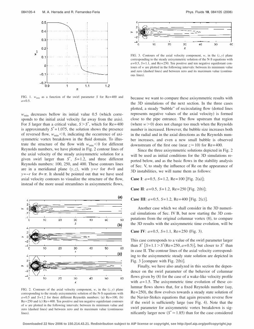
wmin decreases bellow its initial value 0.5 �which corre-sponds to the initial axial velocity far away from the axis�.For S larger than a critical value, S�S*, which for Re=400is approximately S*=1.075, the solution shows the presenceof reversed flow, wmin�0, indicating the occurrence of axi-symmetric vortex breakdown in the fluid domain. To illus-trate the structure of the flow with wmin�0 for differentReynolds numbers, we have plotted in Fig. 2 contour lines ofthe axial velocity of the steady axisymmetric solution for agiven swirl larger than S*, S=1.2, and three differentReynolds numbers: 100, 250, and 400. These contours linesare in a meridianal plane �y ,z�, with y=r for �=0 andy=−r for �=. It should be pointed out that we have usedaxial velocity contours to visualize the structure of the flow,instead of the more usual streamlines in axisymmetric flows,
FIG. 1. wmin as a function of the swirl parameter S for Re=400 anda=0.5.
FIG. 2. Contours of the axial velocity component, w, in the �z ,y� planecorresponding to the steady axisymmetric solution of the N-S equations witha=0.5 and S=1.2 for three different Reynolds numbers: �a� Re=100, �b�Re=250 and �c� Re=400. Ten positive and ten negative equidistant contoursof w are plotted in the following intervals: between its minimum value andzero �dashed lines� and between zero and its maximum value �continuous
lines�.
Downloaded 22 Nov 2006 to 150.214.43.21. Redistribution subject to
because we want to compare these axisymmetric results withthe 3D simulations of the next section. In the three casesplotted, a steady “bubble” of recirculating flow �dotted linesrepresents negative values of the axial velocity� is formedclose to the pipe entrance. The flow upstream that region�where w�0� does not change too much when the Reynoldsnumber is increased. However, the bubble size increases bothin the radial and in the axial directions as the Reynolds num-ber increases, and even a new small bubble is observeddownstream of the first one �near z�10� for Re=400.
Since the three axisymmetric solutions depicted in Fig. 2will be used as initial conditions for the 3D simulations re-ported below, and as the basic flows in the stability analysisof Sec. V, to study the influence of Re on the appearance of3D instabilities, we will name them as follows:
Case I: a=0.5, S=1.2, Re=100 �Fig. 2�a��;
Case II: a=0.5, S=1.2, Re=250 �Fig. 2�b��;
Case III: a=0.5, S=1.2, Re=400 �Fig. 2�c��.
Another case which we shall consider in the 3D numeri-cal simulations of Sec. IV B, but now starting the 3D com-putations from the original columnar vortex �8�, to comparethe 3D results with the axisymmetric time evolution, will be
Case IV: a=0.5, S=1.1, Re=250 �Fig. 3�.
This case corresponds to a value of the swirl parameter largerthan S* �S=1.1�S*�Re=250,a=0.5��, but closer to S* thanin case II. The contour lines of the axial velocity correspond-ing to the axisymmetric steady state solution are depicted inFig. 3 �compare with Fig. 2�b��.
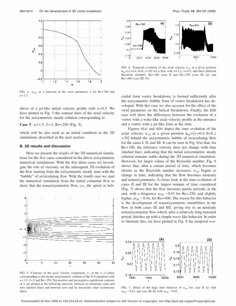
Finally, we have also analyzed in this section the depen-dence on the swirl parameter of the behavior of columnarflows given by �8� for the case of a wake-like velocity profilewith a=1.5. The axisymmetric time evolution of these co-lumnar flows shows that, for a fixed Reynolds number �say,Re=250�, the flow evolves towards a steady state solution ofthe Navier-Stokes equations that again presents reverse flowif the swirl is sufficiently large �see Fig. 4�. Note that theswirl parameter for axisymmetric vortex breakdown is sig-
*
FIG. 3. Contours of the axial velocity component, w, in the �z ,y� planecorresponding to the steady axisymmetric solution of the N-S equations witha=0.5, S=1.1, and Re=250. Ten positive and ten negative equidistant con-tours of w are plotted in the following intervals: between its minimum valueand zero �dashed lines� and between zero and its maximum value �continu-ous lines�.
nificantly larger now �S �1.85� than for the case considered
AIP license or copyright, see http://pof.aip.org/pof/copyright.jsp
084105-5 On the development of 3D vortex breakdown Phys. Fluids 18, 084105 �2006�
above of a jet-like initial velocity profile with a=0.5. Wehave plotted in Fig. 5 the contour lines of the axial velocityfor the axisymmetric steady solution corresponding to
Case V: a=1.5, S=2, Re=250 �Fig. 5�,
which will be also used as an initial condition in the 3Dsimulations described in the next section.
B. 3D results and discussion
Here we present the results of the 3D numerical simula-tions for the five cases considered in the above axisymmetricnumerical simulations. With the first three cases we investi-gate the role of viscosity on the subsequent 3D evolution ofthe flow starting from the axisymmetric steady state with the“bubble” of recirculating flow. With the fourth case we startthe numerical simulation from the initial columnar flow toshow that the nonaxisymmetric flow, i.e., the spiral or heli-
FIG. 4. wmin as a function of the swirl parameter S for Re=250 anda=1.5.
FIG. 5. Contours of the axial velocity component, w, in the �z ,y� planecorresponding to the steady axisymmetric solution of the N-S equations witha=1.5, S=2 and Re=250. Ten positive and ten negative equidistant contoursof w are plotted in the following intervals: between its minimum value andzero �dashed lines� and between zero and its maximum value �continuous
lines�.
Downloaded 22 Nov 2006 to 150.214.43.21. Redistribution subject to
coidal form vortex breakdown, is formed sufficiently afterthe axisymmetric bubble form of vortex breakdown has de-veloped. With this case we also account for the effect of theswirl parameter on the helical breakdown. Finally, the fifthcase will show the differences between the evolution of avortex with a wake-like axial velocity profile at the entranceand a vortex with a jet-like form at the inlet.
Figures 6�a� and 6�b� depict the time evolution of theaxial velocity wref at a given position xref= �r=0.4,�=0,z=30� behind the axisymmetric bubble of recirculating flowfor the cases I, II, and III. It can be seen in Fig. 6�a� that, forRe=100, the reference velocity does not change with time�dashed line�, indicating that the initial axisymmetric steadysolution remains stable during the 3D numerical simulation.However, for larger values of the Reynolds number, Fig. 6shows that, after a certain period of time, which becomesshorter as the Reynolds number increases, wref begins tochange in time, indicating that the flow becomes unsteadyand nonaxisymmetric. A closer look at the time evolution ofcases II and III for the largest instants of time considered�Fig. 7� shows that the flow becomes purely periodic at theend, with a frequency �3D0.43 for Re=250, and slightlyhigher, �3D0.44, for Re=400. The reason for this behavioris the development of nonaxisymmetric instabilities in theflow in both cases �II and III�, giving rise to an unsteadynonaxisymmetric flow which, after a relatively long transientperiod, finishes up with a simple wave-like behavior. In orderto illustrate this, we have plotted in Fig. 8 the temporal evo-
FIG. 6. Temporal evolution of the axial velocity wref at a given positionxref= �r=0.4,�=0,z=30� for a flow with S=1.2, a=0.5, and three differentReynolds numbers: Re=100 �case I� and Re=250 �case II� �a�; andRe=400 �case III� �b�.
FIG. 7. Detail of the large time behavior of wref for: case II �a� with
�3D0.43, and case III �b� with �3D0.44.
AIP license or copyright, see http://pof.aip.org/pof/copyright.jsp
084105-6 M. A. Herrada and R. Fernandez-Feria Phys. Fluids 18, 084105 �2006�
lution of the amplitudes of the different nonaxisymmetricmodes for the axial velocity in the modal decomposition �17�at the same location xref,
An�t� �wn�rref,zref,t��, n � 0. �19�
For Re=250 �Fig. 8�a��, A2 is the first mode that becomesdestabilized, increasing very fast in time, while the ampli-tudes of the other modes begin to increase later and moreslowly. Eventually, for a sufficiently large time, the ampli-tude A2 decays, and the mode corresponding to A1 becomesthe dominant one at the final state �the amplitude A3 andthose corresponding to higher modes not shown in the figureremain always very small�. For Re=400, Fig. 8�b� shows thatthe nonaxisymmetric perturbations develop appreciablyfaster than for Re=250. In addition, the time required for theamplitudes of the nonaxisymmetric modes to reach the finalpurely oscillatory state is much larger. Another significantdifference in this case is that the amplitude A1 is appreciablylarger that A2 from the beginning of the 3D instability, andremains so until the final state.
FIG. 8. Temporal evolution of the different amplitudes An �defined in Eq.�19�� for different nonaxisymmetric modes n�0 corresponding to case II �a�and case III �b�. The inset in �a� is shown to compute the frequency of themode n=2 at its initial stages of development.
FIG. 9. Three-dimensional perspectives of the perturbations of the circula-tion corresponding to case II at time t=4800. �a� Isosurface of �p, �b� iso-surface of the �n � =1 component, and �c� isosurface of the �n � =2 component.
All the isosurfaces are chosen at 10% of their maximum values.
Downloaded 22 Nov 2006 to 150.214.43.21. Redistribution subject to
The above results suggest that, in case II �Re=250�, theflow first develops a double helicoidal structure behind thebubble �the mode n=2 is the dominant one at the beginningof the 3D instability�, evolving later towards a nearly singlehelicoidal structure �n=1�. However, in case III �Re=400�,the mode n=1 seems to be the dominant one from the be-ginning of the instability, but with a significant contributionof the mode n=2 remaining. In order to corroborate thispicture, we have plotted in Figs. 9–11 several isosurfaces ofthe circulation �=rv at different instants of time. In particu-lar, we have used the modal decomposition �17� to expressthe circulation as the sum of an axisymmetric main part anda nonaxisymmetric perturbation,
��r,�,z,t� = �o�r,z,t� + �n�0
�n�r,z,t�exp�in��
�main�r,z,t� + �p�r,�,z,t� . �20�
Figure 9 shows three-dimensional perspectives of the pertur-bation �p of the circulation for case II at the time t=4800
FIG. 10. As in Fig. 9, but for t=8000.
FIG. 11. As in Fig. 9, but for case III at t=7000.
AIP license or copyright, see http://pof.aip.org/pof/copyright.jsp
084105-7 On the development of 3D vortex breakdown Phys. Fluids 18, 084105 �2006�
for which, according to Fig. 8�a�, both modes �n � =1 and�n � =2 are present in the flow at approximately the samelevel. Figure 9�a� displays an isosurface of the whole pertur-bation �p corresponding to the 10% of its maximum value,while Figs. 9�b� and 9�c� display the isosurfaces for its�n � =1 and �n � =2 components, respectively �both corre-sponding to the 10% of their respective maximum values�.The double-helicoidal structure of the flow is clear in Fig.9�a�, but it is distorted in relation to the pure mode �n � =2,depicted in Fig. 9�c�, due to the relative importance of thecomponent �n � =1 �Fig. 9�b��. For subsequent times, the rela-tive importance of the mode �n � =2 decays and, for t=8000�Fig. 10�, the downstream flow corresponds to an almostsingle helical structure �note that Figs. 10�a� and 10�b� arepractically coincident�.
FIG. 12. Contour lines of �p on the �� ,z� plane for r=rref=0.4 and for twodifferent instants of time ��a� t=4900 and �b� t=8000� for case II. Fivepositive and five negative equidistant contours of �p are plotted in the fol-lowing intervals: between its minimum value and zero �dashed lines� andbetween zero and its maximum value �continuous lines�.
FIG. 13. As in Fig. 12, but for case III at t=7000 �a�, and at t=10000 �b�.
Downloaded 22 Nov 2006 to 150.214.43.21. Redistribution subject to
Figure 11 shows three-dimensional perspectives of theperturbation of the circulation for case III �Re=400� att=7000. The structure of the flow �Fig. 11�a�� is a mixingof the mode �n � =1 �Fig. 11�b�� and the mode �n � =2�Fig. 11�c��. However, for larger times, the situation is simi-lar to case II, becoming the mode �n � =1 the dominant one.
To find out the winding direction of the helicoidal, or thedouble helicoidal, vortex breakdown structures appearing inthe wake of the axisymmetric breakdown bubble during thetemporal evolution of the flow, one may use the contour linesof the nonaxisymmetric part of the circulation �p in a plane�� ,z� for some value of r at several instants of time. Figure12 shows these contour lines at r=rref=0.4 for case II �Re=250� at t=4900 and at t=8000. For t=4900 �Fig. 12�a��, theinclination of the contour lines in the region 5�z�10 �ap-proximately� indicates negative values of the azimuthal wavenumbers, while the change in the inclination of the contoursin the main downstream region 10�z�60 indicates positivevalues of n. However, for t=8000 �Fig. 12�b��, almost all the
FIG. 14. Contour lines of the axial velocity component, w, on the �z ,y�plane of the 3D solution for: �a� case II at t=8000, and �b� case III att=10000. Ten positive and ten negative equidistant contours of w are plottedin the following intervals: between its minimum value and zero �dashedlines� and between zero and its maximum value �continuous lines�.
FIG. 15. Comparison between the time evolution of the axial velocity, wref,at the fixed position xref, obtained from the 3D numerical simulation �solidline� and from the axisymmetric one �dashed line� for case IV. Part �a�shows the whole evolution from the initial columnar flow, and part �b�the periodic character of the resulting 3D flow at the final stages with
�3D0.37.
AIP license or copyright, see http://pof.aip.org/pof/copyright.jsp
084105-8 M. A. Herrada and R. Fernandez-Feria Phys. Fluids 18, 084105 �2006�
contour lines have the same �positive� slope, n�0. Theseresults suggest that several types of nonaxisymmetric insta-bilities develop in the flow �both with n�0 and with n�0�,but only the perturbations with n�0 remain for sufficientlylarge times. Figure 13 shows the contour lines of �p in the�� ,z� plane at r=rref=0.4 for case III �Re=400� at t=7000and at t=10000. The situation in this case is quite similar tothat observed for Re=250: waves with n�0 and n�0 de-velop in the flow, but only the n�0 ones, particularly withn= +1, survive at later times.
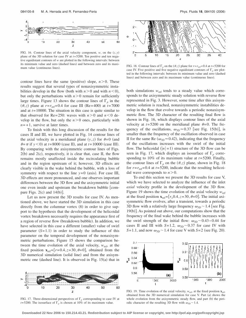
To finish with this long discussion of the results for thecases II and III, we have plotted in Fig. 14 contour lines ofthe axial velocity in a meridianal plane �y ,z� for �=0 �and�= if y�0� at t=8000 �case II�, and at t=10000 �case III�.By comparing with the axisymmetric contour lines of Figs.2�b� and 2�c�, respectively, it is clear that, case II, the flowremains mostly unaffected inside the recirculating bubbleand in the region upstream of it; however, 3D effects areclearly visible in the wake behind the bubble, with a loss ofsymmetry with respect to the line y=0 �axis�. For case III,3D effects are more pronounced, and one observes importantdifferences between the 3D flow and the axisymmetric initialone even inside and upstream the breakdown bubble �com-pare Figs. 2�c� and 14�b��.
Let us now present the 3D results for case IV. As men-tioned above, we have started the 3D simulation in this casedirectly from the columnar vortex �8� in order to give sup-port to the hypothesis that the development of the helicoidalvortex breakdown necessarily requires the appearance first ofa region of reverse flow �breakdown bubble�. In addition, wehave selected in this case a different �smaller� value of swirlparameter �S=1.1� in order to study the influence of thisparameter on the temporal development of the nonaxisym-metric perturbations. Figure 15 shows the comparison be-tween the time evolution of the axial velocity, wref, at thefixed position xref= �r=0.4,z=30,�=0�, obtained from the3D numerical simulation �solid line� and from the axisym-metric one �dashed line�. It is observed in Fig. 15�a� that in
FIG. 16. Contour lines of the axial velocity component, w, on the �z ,y�plane of the 3D solution for case IV at t=5200. Ten positive and ten nega-tive equidistant contours of w are plotted in the following intervals: betweenits minimum value and zero �dashed lines� and between zero and its maxi-mum value �continuous lines�.
FIG. 17. Three-dimensional perspectives of �p corresponding to case IV at
t=5200. The isosurface of �p is chosen at 10% of its maximum value.
Downloaded 22 Nov 2006 to 150.214.43.21. Redistribution subject to
both simulations wref tends to a steady value which corre-sponds to the axisymmetric steady solution with reverse flowrepresented in Fig. 3. However, some time after this axisym-metric solution is reached, nonaxisymmetric instabilities de-velop in the flow that evolve towards a periodic nonaxisym-metric flow. The 3D character of the resulting final flow isshown in Fig. 16, which displays contour lines of the axialvelocity at t=5200 on the meridianal plane �=0. The fre-quency of the oscillations, �3D�0.37 �see Fig. 15�b��, issmaller than the frequency of the oscillation observed in caseII for the same Re ��3D�0.42�, indicating that the frequencyof the oscillations increases with the swirl of the initialflow. The helicoidal ��n � =1� structure of the 3D flow can beseen in Fig. 17, which displays an isosurface of �p corre-sponding to 10% of its maximum value at t=5200. Finally,the contour lines of �p on the �� ,z� plane, shown in Fig. 18for r=rref=0.4 at t=5200, indicate that the resulting helicoi-dal wave corresponds to n�0.
To end this section we present the 3D results for case V,which we have selected to analyze the influence of the inletaxial velocity profile in the development of the 3D flow.Figure 19 shows the time evolution of the axial velocity wref
at the fixed position xref= �r=0.4,z=30,�=0�. The initial axi-symmetric flow evolves, after a transient, towards a periodic3D flow with a relatively large frequency �3D1.4 �see Fig.19�b��. As pointed out above, our computations show that thefrequency of the final wake behind the bubble increases withthe swirl strength of the initial flow: �3D0.43−0.44 forcases II and III with S=1.2, �3D0.37 for case IV withS=1.1, and now �3D1.4 for case V with S=2 �see Fig. 20�.
FIG. 18. Contour lines of �p on the �� ,z� plane for r=rref=0.4 at t=5200 forcase IV. Five positive and five negative equidistant contours of �p are plot-ted in the following intervals: between its minimum value and zero �dashedlines� and between zero and its maximum value �continuous lines�.
FIG. 19. Time evolution of the axial velocity, wref, at the fixed position xref,obtained from the 3D numerical simulation for case V. Part �a� shows thewhole evolution from the axisymmetric steady flow, and part �b� the peri-
odic character of the resulting 3D flow with �3D1.4.
AIP license or copyright, see http://pof.aip.org/pof/copyright.jsp
084105-9 On the development of 3D vortex breakdown Phys. Fluids 18, 084105 �2006�
The 3D character of the resulting flow is shown in Fig. 21,that displays contour lines of the axial velocity at t=2000. Itmay be noted the large differences between the resulting 3Dflow and the initial axisymmetric flow �Fig. 5�. In particular,the region of reverse flow completely disappear during the3D evolution �there is no negative axial velocity in the wholedomain�. This result is qualitatively different from the resultsobtained for cases II, III, and IV with a jet-like velocityprofile at the inlet, for which the 3D evolution always pre-serves �though distorted� the bubble of reverse flow near theentrance of the pipe. Following with the presentation of theresults for case V, the helicoidal structure of the flow can beseen in Fig. 22, that displays the isosurfaces of �p �Fig.22�a��, and its components for the modes �n � =1 �Fig. 22�b��,and �n � =2 �Fig. 22�c��, all of them corresponding to the 10%of their respective maximum values at t=2000. The resultingwake flow presents a superposition of helicoidal and double-
FIG. 20. Numerical frequency �3D as a function of S for Re=250. Thecircles correspond to the frequencies obtained in the 3D numerical simula-tions for the cases indicates in the figure.
FIG. 21. Contour lines of the axial velocity component, w, on the �z ,y�plane of the 3D solution for case V at t=5200. Ten positive equidistantcontours of w are plotted in the interval between zero and its maximum
value �no recirculating flow remains�.
Downloaded 22 Nov 2006 to 150.214.43.21. Redistribution subject to
helicoidal waves, but with a single helical flow ��n � =1� ex-iting the pipe. The maximum amplitude ratio between modes�n � =2 and �n � =1 is just 0.00596. Finally, the contour lines of�p in the �� ,z� plane, shown in Fig. 23 for r=rref=0.4 att=2000, indicates that n�0 �n= +1�.
V. LOCAL STABILITY ANALYSIS
A. Formulation of the problem
The full Navier-Stokes numerical simulations of the pre-vious section strongly suggest that the helical vortex break-down structures develop only after a recirculating axisym-metric bubble has been formed in the transient evolution ofthe flow. Following the ideas of Pier and Huerre,17,18 whohave recently shown that the self-sustained nonlinear oscil-lating frequency of wake-like velocity profiles can be deter-mined by the absolute frequency of the local stability analy-sis, we have performed here a linear absolute-convectiveanalysis of those axisymmetric flows which presents a recir-culating bubble. By means of a simple linear, spatial stabilityanalysis carried out in the sections of the pipe where theintermediate axisymmetric flow presents reverse flow �nega-
FIG. 22. Three-dimensional perspectives of the perturbations of the circu-lation corresponding to case V at t=2000. �a� Isosurface of �p, �b� isosurfaceof the mode with �n � =1, and �c� isosurface of the mode with �n � =2. All theisosurfaces are chosen at 10% of their maximum values.
FIG. 23. Contour lines of �p on the �� ,z� plane for r=rref=0.4 for case V att=2000. Five positive and five negative equidistant contours of �p are plot-ted in the following intervals: between its minimum value and zero �dashed
lines� and between zero and its maximum value �continuous lines�.
AIP license or copyright, see http://pof.aip.org/pof/copyright.jsp
084105-10 M. A. Herrada and R. Fernandez-Feria Phys. Fluids 18, 084105 �2006�
tive axial velocity at the axis�, we have tried to identify thefrequencies and the dominant azimuthal wave numbers ob-served in the 3D simulations.
We first proceed to decompose both the velocity andpressure fields in a basic part, Uo= �Uo ,Vo ,Wo� and Po, and aperturbation, u�= �u� ,v� ,w�� and p�,
u = Uo + u�, v = Vo + v�, w = Wo + w�, p = Po + p�,
�21�
where the basic flow corresponds to any of the previouslycomputed axisymmetric steady solutions of the N-S equa-tions considered above �cases I–V�, all of them with a regionof reverse flow. Taking into account that in our simulationsRe�1, we use the method of multiple scales by introducinga slow axial variable Z=z /Re, and by expressing the un-steady perturbations in terms of a slowly varying amplitudeand axial wave number in the form
�u�,p���z,r,�,t� = �n
�un,pn��Z,r�
�exp�Re�Z
kn���d� + in� − i�t� .
�22�
In this expression, n is the azimuthal wave number, while��� /wc and kn�Kn are the nondimensional frequencyand axial wave numbers, respectively, being � and Kn thecorresponding dimensional values. We will perform a spatialstability analysis, where � is real and the kn are complexnumbers. The real and the imaginary parts, � and �, of thecomplex axial wave number,
kn �n + i�n, �23�
are the exponential growth rate and the axial wave number,respectively, for each n.
Introducing �22� into the Navier-Stokes equations�1�–�4�, retaining only linear terms of the perturbations, ne-glecting terms of order �1/Re�2 and the nonparallel termsarising from the axial variation of both the basic and pertur-bated flows, one arrives at the following set of linear equa-tions for the amplitude of the perturbations:
wnkn +�un
�r+
un
r+
invn
r= 0, �24�
i�un − knWoun − Uo�un
�r− un
�Uo
�r−
�pn
�r
+1
Re� �2un
�r2 +1
r
�un
�r+ �kn
2 −n2
r2 �un −un
r2 − 2invn
r2� = 0,
�25�
i�vn − knWovn − Uo�vn
�r− Uo
vn
r− in
pn
r
+1
Re� �2vn
�r2 +1
r
�vn
�r+ �kn
2 −n2
r2 �vn + 2inun
r2 −vn
r2� = 0,
�26�
Downloaded 22 Nov 2006 to 150.214.43.21. Redistribution subject to
i�wn − knWown − Uo�wn
�r− un
�Wo
�r− knpn
+1
Re� �2wn
�r2 +1
r
�wn
�r+ �kn
2 −n2
r2 �wn� = 0. �27�
By neglecting the nonparallel terms �near-parallel approxi-mation�, the global stability problem is reduced to a localstability analysis to be solve at different z stations.
The system have been solved subjected to the followingradial boundary conditions for each azimuthal wavenumber n:
at r = Ro, un = vn = �rwn = 0; �28�
at r = 0, un = vn = 0, �rwn = 0 �n = 0� ,
un ± ivn = 0, �run = 0, wn = 0 �n = ± 1� ,
un = vn = wn = 0 ��n� � 1� .
�29�
Note that it is assumed that the perturbations do not modifythe basic flow at the pipe wall r=Ro, and satisfy the sameboundary condition as the basic flow at the axis. Observe,however, that the stability equations are not symmetric withrespect to n �since the basic swirl velocity vo is not zero�, andtherefore both positive and negative azimuthal wave num-bers n have to be considered.
B. Numerical scheme
It proves convenient to rewrite Eqs. �24�–�27� in theform
0 = �L1 + knL2 +kn
2
ReL3� · S , �30�
where L1, L2, and L3 are complex matrices which depend onz �only through the basic flow� and r, and S�un , pn�. Tosolve �30� numerically, the equations are discretized in the rdirection using the same Chebyshev spectral collocationtechnique employed in the full numerical simulations. Thenonlinear �quadratic� eigenvalue problem �30� for kn issolved using the linear companion matrix method describedin Ref. 28. The resulting linear eigenvalue problem is nu-merically solved with the help of an eigenvalue solver sub-routine DGVCCG from the IMSL library, which provides theentire spectrum of eigenvalues and eigenfunctions. Spuriouseigenvalues were ruled out by comparing the computed spec-trums obtained for different values of the number of colloca-tion points nr. For most of the computations reported below,values of nr between 31 and 41 were enough to obtain theeigenvalues with at least 7 significant figures, as it waschecked out for every result given below by using largervalues of nr.
C. Results
We have applied the above lineal stability analysis to thebasic axisymmetric flows considered in the numerical simu-lations of Sec. IV A �cases I–V�, all of them with a region of
reverse flow close to the pipe inlet. Since the stability analy-
AIP license or copyright, see http://pof.aip.org/pof/copyright.jsp
084105-11 On the development of 3D vortex breakdown Phys. Fluids 18, 084105 �2006�
sis that we propose here is local, one important preliminaryquestion is the selection of the axial station to perform thestability analysis in order to predict the main 3D features ofthe subsequent flow. We have seen in the 3D simulations ofthe previous section that the flow develops a helicoidal struc-ture only after a region of reverse flow �axisymmetric break-down bubble� is present in the domain. This fact suggests usthe idea of carrying out the stability analysis at the z stationwhere the axial velocity of the axisymmetric basic flowreaches its minimum �negative� value, that will be designedby z*. Figure 24 shows the axial �solid lines� and azimuthal�dashed lines� velocity profiles of the basic axisymmetricflows corresponding to the five cases considered as functionsof r at z=z* �the corresponding values of z* are indicated inthe respective figures; see also Figs. 2, 3, and 5�. As we shallsee, the local stability analysis applied to these velocity pro-files predicts surprisingly well the existence and the proper-ties of the subsequent 3D wake, provided that the flow isabsolutely unstable. As a matter of fact, to apply the empiri-cal frequency selection of Pierrehumbert,19 one should exam-ine the existence of absolute instabilities regions in the wholeaxisymmetric flow, particularly inside the bubble region offlow reverse, and look for the most �absolutely� unstable per-turbation. But, as we show below, this most unstable pertur-bation is located at, or very close to, the axial station wherethe axial velocity presents its minimum �negative� value.
For a given azimuthal wave number n and for real fre-quencies � �spatial stability analysis�, we solve Eq. �30� toobtain the complete eigenvalue spectrum. Let us start withcase I �velocity profiles at z=z* given in Fig. 24�a��. Follow-ing the definitions of convective and absolute instabilitiesgiven by Huerre and Monkewitz,29 we find that the flow isonly convectively unstable for perturbations with n=1. Thiscan be seen in Fig. 25, where we have plotted � and � asfunctions of � for the most unstable modes �largest growth
FIG. 24. Axial �continuous line� and azimuthal �dashed line� velocities pro-files of the basic flow at the axial position z=z* where the local stabilityanalysis is carried out, case I �a�, case II �b�, case III �c�, case IV �d�, andcase V �e�.
rate �� with n=1. Observe that � increases with � �Fig.
Downloaded 22 Nov 2006 to 150.214.43.21. Redistribution subject to
25�a��, indicating that the group velocity is always positive,and that the growth rate is positive in a certain range offrequencies �Fig. 25�b��. Therefore, the amplitude of any per-turbation with n=1 and with a frequency in that range growsas z increases. In the full numerical simulations for this caseperformed in Sec. IV B we have not appreciated the spatialgrowth of any nonaxisymmetric perturbation. This can bedue to the fact that the spatial growth rates are quite small, sothat a much longer pipe would be necessary to appreciate thedownstream amplification of just the numerical noise to vi-sualize these convective instabilities �in the form of travel-ling waves� in that specific range of frequencies.
The situation is qualitatively different for the rest of thecases depicted in Figs. 24�b�–24�d� �cases II–V�, where thevelocity profiles are found to be not just convectively un-stable, but also absolutely unstable. To find out these abso-lute instabilities one should look for the presence of saddlepoints in the dispersion relation, arising from the coalescenceof two spatial branches located at opposite sides of the �� ,��plane �Briggs-Bers criterion; see, e.g., Huerre andMonkewitz29 and, for a more recent account, Chomaz30�. Byvarying the imaginary part of the frequency, �i, we havefound a number of such saddle points for the four casesconsidered and for different values of the azimuthal wavenumber n. The main results are compiled in Table I. Therewe show the critical values of the real part of the frequency,�*, the imaginary part of the frequency �absolute growthrate�, �i
*, and the corresponding values of �* and �* at which
FIG. 25. ���� �a� and ���� �b� for the most unstable mode with n=1corresponding to case I.
TABLE I. Absolute instabilities: Characteristics of all the saddle points inthe dispersion relations found in the different cases considered.
Case n �* �* �* �i*
II −1 0.242 1.6 0.6 −0.0245
II +1 0.38 1.8 1.7 −0.128
II +2 0.43 0.85 0.25 +0.021
III −1 0.215 1.52 0.45 −0.0075
III +1 0.435 0.5 3.3 +0.012
III +2 0.4104 0.22 0.1 −0.0195
IV +1 0.35 0.46 5.6 +0.0435
IV +2 0.59 0.8 0.9 +0.009
V −1 1.8 0.3 3.3 +0.16
V +1 1.3 1.5 0.8 +0.31
V +2 2.4 1. 1.5 −0.052
AIP license or copyright, see http://pof.aip.org/pof/copyright.jsp
084105-12 M. A. Herrada and R. Fernandez-Feria Phys. Fluids 18, 084105 �2006�
these saddle points in the dispersion relation are found. Notethat only five of these cases correspond to absolute instabili-ties, those for which the imaginary part of the frequency ispositive ��i
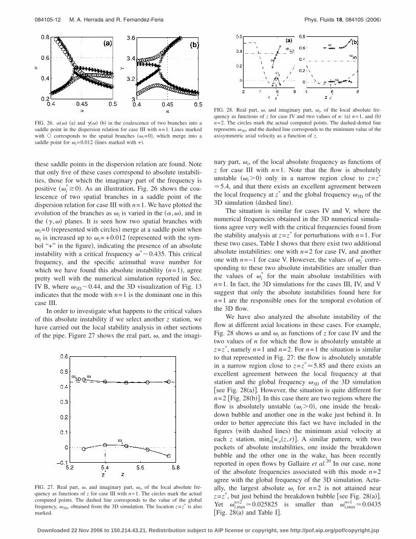
*�0�. As an illustration, Fig. 26 shows the coa-lescence of two spatial branches in a saddle point of thedispersion relation for case III with n=1. We have plotted theevolution of the branches as �i is varied in the �� ,��, and inthe �� ,�� planes. It is seen how two spatial branches with�i=0 �represented with circles� merge at a saddle point when�i is increased up to �i= +0.012 �represented with the sym-bol “+” in the figure�, indicating the presence of an absoluteinstability with a critical frequency �*0.435. This criticalfrequency, and the specific azimuthal wave number forwhich we have found this absolute instability �n=1�, agreepretty well with the numerical simulation reported in Sec.IV B, where �3D0.44, and the 3D visualization of Fig. 13indicates that the mode with n=1 is the dominant one in thiscase III.
In order to investigate what happens to the critical valuesof this absolute instability if we select another z station, wehave carried out the local stability analysis in other sectionsof the pipe. Figure 27 shows the real part, �, and the imagi-
FIG. 26. ���� �a� and ���� �b� in the coalescence of two branches into asaddle point in the dispersion relation for case III with n=1. Lines markedwith � corresponds to the spatial branches ��i=0�, which merge into asaddle point for �i=0.012 �lines marked with +�.
FIG. 27. Real part, �, and imaginary part, �i, of the local absolute fre-quency as functions of z for case III with n=1. The circles mark the actualcomputed points. The dashed line corresponds to the value of the globalfrequency, �3D, obtained from the 3D simulation. The location z=z* is also
marked.
Downloaded 22 Nov 2006 to 150.214.43.21. Redistribution subject to
nary part, �i, of the local absolute frequency as functions ofz for case III with n=1. Note that the flow is absolutelyunstable ��i�0� only in a narrow region close to z=z*
�5.4, and that there exists an excellent agreement betweenthe local frequency at z* and the global frequency �3D of the3D simulation �dashed line�.
The situation is similar for cases IV and V, where thenumerical frequencies obtained in the 3D numerical simula-tions agree very well with the critical frequencies found fromthe stability analysis at z=z* for perturbations with n=1. Forthese two cases, Table I shows that there exist two additionalabsolute instabilities: one with n=2 for case IV, and anotherone with n=−1 for case V. However, the values of �i
* corre-sponding to these two absolute instabilities are smaller thanthe values of �i
* for the main absolute instabilities withn=1. In fact, the 3D simulations for the cases III, IV, and Vsuggest that only the absolute instabilities found here forn=1 are the responsible ones for the temporal evolution ofthe 3D flow.
We have also analyzed the absolute instability of theflow at different axial locations in these cases. For example,Fig. 28 shows � and �i as functions of z for case IV and thetwo values of n for which the flow is absolutely unstable atz=z*, namely n=1 and n=2. For n=1 the situation is similarto that represented in Fig. 27: the flow is absolutely unstablein a narrow region close to z=z*�5.85 and there exists anexcellent agreement between the local frequency at thatstation and the global frequency �3D of the 3D simulation�see Fig. 28�a��. However, the situation is quite different forn=2 �Fig. 28�b��. In this case there are two regions where theflow is absolutely unstable ��i�0�, one inside the break-down bubble and another one in the wake just behind it. Inorder to better appreciate this fact we have included in thefigures �with dashed lines� the minimum axial velocity ateach z station, minr�wo�z ,r��. A similar pattern, with twopockets of absolute instabilities, one inside the breakdownbubble and the other one in the wake, has been recentlyreported in open flows by Gallaire et al.20 In our case, noneof the absolute frequencies associated with this mode n=2agree with the global frequency of the 3D simulation. Actu-ally, the largest absolute �i for n=2 is not attained nearz=z*, but just behind the breakdown bubble �see Fig. 28�a��.Yet �i,max
n=2 �0.025825 is smaller than �i,maxn=1 �0.0435
FIG. 28. Real part, �, and imaginary part, �i, of the local absolute fre-quency as functions of z for case IV and two values of n: �a� n=1, and �b�n=2. The circles mark the actual computed points. The dashed-dotted linerepresents �3D, and the dashed line corresponds to the minimum value of theaxisymmetric axial velocity as a function of z.
�Fig. 28�a� and Table I�.
AIP license or copyright, see http://pof.aip.org/pof/copyright.jsp
084105-13 On the development of 3D vortex breakdown Phys. Fluids 18, 084105 �2006�
As discussed above for cases III and IV with n=1, wehave also found a unique region of absolute instability forthe most unstable mode for case V, which is also very closeto the z station where the axial velocity presents a minimumvalue inside the breakdown bubble �see Fig. 29�. As a differ-ence with cases III and IV, the frequency �3D found in the3D numerical simulations does not corresponds exactly tothe largest absolute growth rate, but corresponds to a z sta-tion slightly upstream of z*, while the location of the largest�i is a bit downstream of z*. It is worth noticing that in thiscase V, with a wake-like velocity profile at the inlet, theabsolute growth rates are much larger than in the previouslydiscussed cases.
Let us finish with the discussion of the stability resultsfor case II, which is slightly different to the previous ones.The local stability analysis at z=z* shows that there exists anabsolute instability for n=2 �see Table I�, with a critical fre-quency �*0.43. The complementary analysis of the abso-lute instability of the flow at different axial locations for thiscase is shown in Fig. 30. Note that, although the largestabsolute frequency, �i,max
n=2 , is not attained at z=z*, but at aslightly downstream position, there exists again an excellentagreement between the local frequency at z* and the globalfrequency �3D of the 3D numerical simulation once the pe-riodic flow is fully developed. This case is particularly inter-esting because the long time amplitude of the 3D wavesobserved in the 3D simulations does not correspond to themode n=2, but to the mode n=1. In fact, the temporal evo-lution of the 3D flow shows that, at the initial stages, themode with n=2 is the dominant one �see Figs. 8�a� and 9�,just as the local stability analysis predicts, with a frequencyof the oscillations at t=2100 given by �3D
t=2100�0.53 �seeinset in Fig. 8�a��, which coincides with the critical fre-quency of the local stability analysis at the z station where�i,max
n=2 is attained �see Fig. 30�. However, for larger times, theamplitude of the mode with n=2 decays, while the amplitudeof mode with n=1 increases drastically, becoming the domi-nant one in the 3D simulations �see Figs. 8�a� and 10�. Thefinal frequency of the flow coincides however with the fre-quency obtained from the stability analysis for the moden=2 at z=z*. All this suggests that nonlinear effects, that are
FIG. 29. Real part, �, and imaginary part, �i, of the local absolute fre-quency as functions of z for case V with n=1. The dashed line marks thevalue of the global frequency, �3D, obtained from the 3D simulation. Thelocation z=z* is also marked.
obviously not taken into account in the linear stability analy-
Downloaded 22 Nov 2006 to 150.214.43.21. Redistribution subject to
sis, may account for this change in the 3D structure of theflow from the mode with n=2 to the mode with n=1, oncethe first absolute instability with n=2 predicted by the localstability analysis develops in the flow.
VI. CONCLUSIONS
Three-dimensional and axisymmetric numerical simula-tions of the incompressible Navier-Stokes equations havebeen conducted to study the appearance and development ofvortex breakdown in a family of columnar vortex flows in-side a straight pipe without wall friction for several values ofthe Reynolds number. Both types of numerical simulations�axisymmetric and 3D� show that the columnar flow evolvestowards an axisymmetric flow with a closed region of re-verse flow if the relative strength of the swirl is sufficientlyhigh. This means that, in the 3D scenario considered in thiswork, vortex breakdown can be viewed as a transition from acolumnar axisymmetric swirling flow to a basic form of vor-tex breakdown which is axisymmetric �“bubble” break-down�. However our numerical simulations suggest thatthese axisymmetric “bubble” breakdown structures are un-stable under infinitesimal, nonaxisymmetric perturbations ifthe Reynolds number is large enough. Thus, a transition tohelical vortex breakdown modes is observed in the 3D simu-lations after the axisymmetric bubble structure is formed.The final solution at large time is a superposition of a steadyaxisymmetric flow and a helicoidal, and/or double-helicoidal, standing waves with a characteristic frequency ofoscillation. We have also analyzed the role of the swirl pa-rameter S, and of the jet- or wake-like nature of the axialvelocity profile selected at the inlet of the pipe �characterizedby the parameter a� in the development of these helical struc-tures. The numerical simulations demonstrate that the fre-quency of the helical flows increases with the swirl param-
FIG. 30. Real part, �, and imaginary part, �i, of the local absolute fre-quency as functions of z for case II with n=2. The dashed line marks thevalue �3D of the frequency obtained from the 3D numerical simulation forlarge times, while the dotted-dashed line marks the value �3D
t=2100 of thefrequency of the mode n=2 at its initial stages �t=2100; see inset inFig. 8�a��.
eter S �see Fig. 20�. For jet-like velocity profiles at the inlet
AIP license or copyright, see http://pof.aip.org/pof/copyright.jsp
084105-14 M. A. Herrada and R. Fernandez-Feria Phys. Fluids 18, 084105 �2006�
�a�1�, the 3D evolution of the flow preserves the region ofreverse flow near the entrance of the pipe, which remainsalmost axisymmetric, while for wake-like inlet flows �a�1�, the region of reverse flow near the entrance disappears.The helicoidal winding sign of the wakes found in this work�n�0� agrees with the reported by Ruith et al.14 in openvortices. In both cases, all the waves found in the 3D numeri-cal simulations wind in opposite direction to the main flow.
We show here that the development of the helicoidalvortex breakdown structures in the flow is caused by apocket of absolute instability inside the axisymmetric bubbleof recirculating flow formed at the initial stages of the evo-lution of the flow. By means of a simple spatial, linear sta-bility analysis carried out locally at the section where thebasic axisymmetric flow present a �negative� minimum in theaxial velocity at the axis, we have first shown that no 3Dwakes develop when the flow is stable or just convectivelyunstable at these axial locations. This situation occurs forrelatively low Reynolds numbers �case I considered in thiswork�. When the Reynolds number is large enough, we haverelated the frequencies and the dominant azimuthal wavenumbers observed in the 3D simulations with the criticalfrequencies, and the corresponding azimuthal wave numbers,of the absolute instabilities found at these axial stations. Al-though we have not make an exhaustive analysis owing tothe enormous computational effort required by each 3D nu-merical simulation, the results are quite encouraging: in allthe four cases where a helicoidal structure is found in thenumerical simulation, the local stability analysis predictswith pretty good precision the frequency of the oscillationsin the standing lee wave, and the value of the dominant azi-muthal wave number. In one of the cases considered �caseII�, this good agreement is found only at the initial stages ofthe 3D evolution of the flow; afterwards, the flow evolves“nonlinearly” to a different helical structure which, obvi-ously, cannot be predicted by the present linear stabilityanalysis. But, surprisingly, the final frequency of the flowcoincides with the frequency obtained from the stabilityanalysis. It is interesting to emphasize here that the stabilityanalyses are performed locally at the axial stations where theaxial velocity presents a minimum �negative� value insidethe bubble or recirculating flow formed by the initial axisym-metric vortex breakdown. To our knowledge, no such asimple criterion to predict 3D vortex breakdown structures,nor its detailed development from an axisymmetric form ofvortex breakdown, have been previously reported, though therelation between vortex breakdown and absolute instabilitieshas been extensively debated for several types of swirlingflows.14,31–35
Similar results, but in the context of bluff-body wakes,and considering the stability analysis in a finite region insidethe near field of the wake just behind the body, have beenrecently reported by Pier and Huerre,17,18 and by Sevilla andMartinez-Bazan,36 among others. Finally to mention the re-cent work by Gallaire et al.,20 where similar ideas are devel-oped for open vortices. However, in contrast to the presentresults, these authors find two pockets of absolute instabilityfor the dominant mode, one in the breakdown bubble and the
other one in the wake behind it. Here, in all the cases con-
Downloaded 22 Nov 2006 to 150.214.43.21. Redistribution subject to
sidered, there is an unique region of absolute instability forthe dominant mode inside the breakdown bubble, with themost absolutely unstable station close to the location wherethe axial velocity of the axisymmetric flow presents its mini-mum value �z=z*�. This criterion for the frequency selectionbased on the highest absolute growth rate was first proposedby Pierrehumbert19 in the context of baroclinic instabilities,and differ from that given by Pier and Huerre17,18 based onthe frequency at the convective/absolute transition station.However, the frequency predictions by these two criteria arein reasonable agreement in the present problem due to thefact that all the frequencies within the pockets of absoluteinstability are in a relatively narrow range.
ACKNOWLEDGMENTS
This work has been supported by the Ministerio de Edu-cación y Ciencia of Spain through Grants No. DPI2002-04305-C02-02 and No. FIS04-00538. The authors thank theanonymous referees for their valuable comments which haveimproved the quality of the paper.
1M. G. Hall, “Vortex breakdown,” Annu. Rev. Fluid Mech. 4, 195 �1972�.2T. Sarpkaya, “On stationary and travelling vortex breakdowns,” J. FluidMech. 45, 545 �1971�.
3S. Leibovich, “The structure of vortex breakdown,” Annu. Rev. FluidMech. 10, 221 �1978�.
4M. P. Escudier, “Vortex breakdown: observations and explanations,” Prog.Aeronaut. Sci. 25, 189 �1988�.
5O. Lucca-Negro and T. O’Doherty, “Vortex breakdown: a review,” Prog.Energy Combust. Sci. 27, 431 �2001�.
6J. D. Buntine and P. G. Saffman, “Inviscid swirling flows and vortexbreakdown,” Proc. R. Soc. London, Ser. A 449, 139 �1995�.
7S. Wang and Z. Rusak, “The dynamics of a swirling flow in a pipe and thetransition to axisymmetric vortex breakdown,” J. Fluid Mech. 340, 177�1997�.
8R. Fernandez-Feria and J. Ortega-Casanova, “Inviscid vortex breakdownmodels in pipes,” ZAMP 50, 698 �1999�.
9P. S. Beran and F. E. C. Culick, “The role of nonuniqueness in the devel-opment of vortex breakdown in tubes,” J. Fluid Mech. 242, 491 �1992�.
10J. M. Lopez, “On the bifurcation structure of axisymmetric vortex break-down in a constricted pipe,” Phys. Fluids 6, 3683 �1994�.
11Z. Rusak and J. H. Lee, “The effect of compressibility on the critical swirlof vortex flows in a pipe,” J. Fluid Mech. 461, 301 �2002�.
12M. A. Herrada, M. Pérez-Saborid, and A. Barrero, “Vortex breakdown incompressible flows in pipes,” Phys. Fluids 15, 2208 �2003�.
13J. C. Tromp and P. S. Beran, “The role of nonuniqueness axisymmetricsolutions in 3-d vortex breakdown,” Phys. Fluids 9, 992 �1997�.
14M. R. Ruith, P. Chen, E. Meiburg, and T. Maxworhy, “Three-dimensionalvortex breakdown in swirling jets and wakes: direct numerical similation,”J. Fluid Mech. 486, 331 �2003�.
15F. Gallaire and J.-M. Chomaz, “Mode selection in swirling jet experi-ments: a linear stability analysis,” J. Fluid Mech. 494, 223 �1995�.
16H. Liang and T. Maxworthy, “An experimental investigation of swirlingjets,” J. Fluid Mech. 525, 115 �2005�.
17B. Pier and P. Huerre, “Nonlinear self-sustained structures and fronts inspatially developing wake flows,” J. Fluid Mech. 435, 145 �2001�.
18B. Pier, “On the frequency selection of finite-amplitude vortex shedding inthe cylinder wake,” J. Fluid Mech. 458, 407 �2002�.
19R. T. Pierrehumbert, “Local and global baroclinic instability of zonallyvarying flow,” J. Atmos. Sci. 41, 2141 �1984�.
20F. Gallaire, M. R. Ruith, E. Meiburg, J. M. Chomaz, and P. Huerre, “Spiralvortex breakdown as a global mode,” J. Fluid Mech. 549, 71 �2006�.
21J. H. Faler and S. Leibovich, “An experimental map of the internal struc-ture of a vortex breakdown,” J. Fluid Mech. 86, 313 �1977�.
22G. K. Batchelor, “Axial flow in trailing line vortices,” J. Fluid Mech. 20,645 �1964�.
23
Fluid Vortices, edited by S. I. Green �Kluwer, Dordrecht, 1995�.
AIP license or copyright, see http://pof.aip.org/pof/copyright.jsp
084105-15 On the development of 3D vortex breakdown Phys. Fluids 18, 084105 �2006�
24S. A. Orszag, “Fourier series on spheres,” Mon. Weather Rev. 102, 56�1974�.
25J. M. Lopez, F. Marques, and J. Shen, “An efficient spectral-projectionmethod for the Navier-Stokes equations in cylindrical geometries ii. threedimensional cases,” J. Comput. Phys. 176, 401 �2002�.
26R. E. Lynch, J. R. Rice, and D. H. Thomas, “Direct solution of partialdifferential equations by tensor product methods,” Numer. Math. 6, 85�1964�.
27C. Canuto, M. Y. Hussaini, A. Quarteroni, and T. A. Zang, Spectral Meth-ods in Fluid Dynamics �Springer-Verlag, New York, 1988�.
28T. J. Bridges and P. J. Morris, “Differential eigenvalue problems in whichthe parameter appears nonlinearly,” J. Comput. Phys. 55, 437 �1984�.
29P. Huerre and P. A. Monkewitz, “Local and global instabilities in spatiallydeveloping flows,” Annu. Rev. Fluid Mech. 22, 473 �1990�.
30J.-M. Chomaz, “Global instabilities in spatially developing flows: nonnor-mality and nonlinearity,” Annu. Rev. Fluid Mech. 37, 357 �2005�.
Downloaded 22 Nov 2006 to 150.214.43.21. Redistribution subject to
31I. Delbende, J.-M. Chomaz, and P. Huerre, “Absolute/convective instabili-ties in the batchelor vortex: A numerical study of the linear impulse re-sponse,” J. Fluid Mech. 355, 229 �1998�.
32C. Olendraru, A. Sellier, M. Rossi, and P. Huerre, “Inviscid instability ofthe batchelor vortex: Absolute-convective transition and spatial branches,”Phys. Fluids 11, 1805 �1999�.
33T. Loiseleux, I. Delbende, and P. Huerre, “Absolute and convective insta-bilities of a swirling jet/wake shear layer,” Phys. Fluids 12, 375 �2000�.
34X.-Y. Yin, D.-J. Sun, M.-J. Wei, and J.-Z. Wu, “Absolute and convectivecharacter of slender viscous vortices,” Phys. Fluids 12, 1062 �2000�.
35C. Olendraru and A. Sellier, “Viscous effects in the absolute-convectiveinstability of the Batchelor vortex,” J. Fluid Mech. 459, 371 �2002�.
36A. Sevilla and C. Martinez-Bazan, “Vortex shedding in high Reynoldsnumber axisymmetric bluff-body wakes: Local linear instability and glo-bal bleed control,” Phys. Fluids 16, 3460 �2004�.
AIP license or copyright, see http://pof.aip.org/pof/copyright.jsp