On the Equivalence of the KMV and Maximum LikelihoodMethods for Structural Credit Risk Models

Jin-Chuan Duan, Geneviève Gauthier and Jean-Guy Simonato∗

June 15, 2005

Abstract

Moody’s KMV method is a popular commercial implementation of the structural credit riskmodel pioneered by Merton (1974). Among the key features of their implementation procedureis an algorithm for estimating the unobserved asset value and the unknown parameters. Thisestimation method has found its way to the recent academic literature, but has not yet beenformally analyzed in terms of its statistical properties. This paper fills this gap and showsthat, in the context of Merton’s model, the KMV estimates are identical to maximum likelihoodestimates (MLE) developed in Duan (1994). Unlike the MLE method, however, the KMValgorithm is silent about the distributional properties of the estimates and thus ill-suited forstatistical inference. The KMV algorithm also cannot generate estimates for capital-structurespecific parameters. In contrast, the MLE approach is flexible and can be readily applied todifferent structural credit risk models.

Keywords: Credit risk, transformed data, maximum likelihood, financial distress, EM algo-rithm.

JEL classification code: C22, G13.

∗Duan, Rotman School of Management, University of Toronto. Gauthier and Simonato, HEC (Montréal). Duan,Gauthier and Simonato acknowledge the financial support from the Natural Sciences and Engineering ResearchCouncil of Canada (NSERC), Le Fond Québécois de la Recherche sur la société et la culture (FQRSC) and from theSocial Sciences and Humanities Research Council of Canada (SSHRC). This paper benefits from the comments bythe participants at the IMF seminar, the 15th Derivative Securities and Risk Management Conference in WashingtonDC and the 1st Symposium on Econometric Theory and Application in Taipei.

1

1 Introduction

Credit risk modeling has gained increasing prominence over the years. The interest was in a large

part motivated by new regulatory requirements, such as the Basel Accord, which provide strong

incentives for financial institutions to quantitatively measure and manage risks of their corporate

debt portfolios. Financial institutions have thus either developed their own internal models or relied

on third-party software to assess various measures for the credit risks of their portfolios.

There exist two conceptually different modeling approaches to credit risk — structural and

reduced-form. The structural approach is rooted in the seminal paper of Merton (1974) in which

the firm’s asset value is assumed to follow a geometric Brownian motion and the firm’s capital

structure to consist of a zero-coupon debt and common equity. This structural approach then

yields formulas for the value of the risky corporate bond and the default probability of the firm.

The structural approach is conceptually elegant but is laden with implementation problems. As

pointed out in Jarrow and Turnbull (2000), the firm’s asset values are unobservable and the model

parameters (the assets’ expected return and volatility in the case of Merton’s model) are unknown.

Unobservability is, in fact, considered by many to be the major drawback of the structural credit

risk models.

A popular commercial implementation of the structural credit risk model is Moody’s KMV

method. This proprietary software builds on a variation of Merton’s (1974) credit risk model and

prescribes an iterative algorithm which infers, from the firm’s equity price time series, the firm’s

unobserved total asset value and unknown expected return and volatility, which are the quantities

required for computing, for example, credit spread and default probability.1 In addition to its

popularity among financial institutions, the KMV estimation method has also found its way into

the recent academic literature; for example, Vassalou and Xing (2004) use the computed default

probability to study equity returns, Cao, Simin and Zhao (2005) use the computed asset values

and volatilities to examine growth options, and Bharath and Shumway (2004) use the computed

default probability to study forecasting performance. Albeit its popularity, not much is known

about the statistical properties of the KMV estimates. In fact, it is not entirely clear as to whether

this method is statistically sound.

1 It is our understanding that the KMV method subjects the estimates to further proprietary calibrations. TheKMV estimation method discussed in this paper is the one described in Crosbie and Bohn (2003), which is onlyrestricted to the iterative algorithm.

2

In the academic literature, there exist at least three other ways of dealing with the unobservabil-

ity issue. First, a proxy asset value may be computed as the sum of the market value of the firm’s

equity and the book value of liabilities. Examples of using a market value proxy are Brockman and

Turtle (2003) and Eom, et al (2004). The second approach is based on solving a system of equa-

tions; for example in the case of Merton’s model, the equity pricing and volatility formulas form a

system of two equations linking the unknown asset value and asset volatility to the equity value and

equity volatility. This approach originating from Jones, et al (1984) and Ronn and Verma (1986)

has been used extensively in the deposit insurance literature. The third approach put forward in

Duan (1994) is based on maximum likelihood estimation (MLE) which views the observed equity

time series as a transformed data set with the theoretical equity pricing formula serving as the

transformation. This transformed-data MLE method has been applied to several structural models

in Ericsson and Reneby (2003) and Wong and Choi (2004) and adapted to address survivorship in

Duan, et al (2003).

The benefits of using the MLE method are well understood in statistics and econometrics. In the

context of structural credit risk models, its dominance over the two other approaches discussed in

the preceding paragraph has already been documented in Ericsson and Reneby (2003), Duan, et al

(2003) and Wong and Choi (2004). But what statistical properties does the KMV method possess?

This question is of both academic and practical interest because of the method’s popularity. We

show here that the KMV estimates are identical to the maximum likelihood estimates in the case

of Merton’s (1974) model. Our theoretical argument relies on characterizing the KMV method

as an EM algorithm, a well-known approach for obtaining maximum likelihood estimates. The

transformed-data MLE method is a better alternative, however, because statistical inference follows

naturally in that framework. The KMV method, on the other hand, only generates point estimates.

Perhaps more importantly, the KMV method does not work for structural credit risk models that

involve any unknown capital structure parameter(s) such as, for example, the financial distress level

in Brockman and Turtle (2003). The transformed-data MLE approach can still be applied to such

a model to obtain an estimate for the financial distress level along with other model parameters, as

demonstrated in Wong and Choi (2004). In short, the KMV and MLE methods are equivalent only

in a limited sense because they lead to the same point estimates for the specific structural model

of Merton (1974) but differ for more general structural models.

The paper is organized as follows. Section 2 presents an argument showing the equivalence of

3

the KMV and MLE estimator in the Merton (1974) context. We examine the equivalence both

numerically and theoretically and show that the KMV estimator agrees with the transformed-data

MLE estimator but is deficient for the inference purpose. Section 3 discusses the limitations of the

KMV approach. The Brockman and Turtle (2003) model is used there to demonstrate that the

KMV method does not generate the capital-structure specific parameter. Section 4 concludes.

2 Equivalence of the KMV and maximum likelihood estimatesunder Merton’s (1974) model

2.1 Merton’s (1974) model

Merton (1974) derived a risky bond pricing formula using the derivative pricing technology and a

simple capital structure assumption. The firm’s assets are financed by equity and a zero-coupon

debt with a face value of F maturing at time T . The risk-free interest rate r is assumed to be

constant. The market value of assets, equity and risky debt at time t are denoted by Vt, St and

Dt, respectively. Naturally, the following accounting identity holds for every time point :

Vt = St +Dt. (1)

It was further assumed that the asset value follows a geometric Brownian motion :

d lnVt =

µµ− σ2

2

¶dt+ σdWt (2)

where µ and σ are, respectively, the expected return and volatility rates, and Wt is a Wiener

process. The risky debt in this framework is entitled to a time-T cash flow of min {VT , F} whosemarket value prior to time T can be obtained using the standard risk-neutral pricing theory; that

is,

Dt = Fe−r(T−t)µ

VtFe−r(T−t)

Φ (−dt) + Φ³dt − σ

√T − t

´¶(3)

where Φ (•) is the standard normal distribution function and dt = ln(Vt/F )+(r+ 12σ2)(T−t)

σ√T−t . In addition,

the formulas for the conditional default probability and equity value can be readily derived to be :

Pt = Φ

Ãln(F/Vt)−

¡µ− 1

2σ2¢(T − t)

σ√T − t

!, (4)

and

St = VtΦ (dt)− Fe−r(T−t)Φ³dt − σ

√T − t

´. (5)

4

Operationally, one can implement Merton’s (1974) model only if the unobserved asset value, Vt,

and the model parameters, µ and σ, can be reasonably estimated.

2.2 The KMV estimation method

The equity values are observed at regular time points, and we denote the time series of n + 1

observations by {S0, Sh, S2h, · · · , Snh} where h is the length of time, measured in years, betweentwo observations; for example, a time series obtained by sampling on a daily basis over a two-year

period will correspond roughly to h = 1/250 and n = 500.

The key to understanding the KMV method is that the unobserved asset value corresponding

to a given observed equity value can be implied out from the equity pricing equation (5) if the

asset volatility is known. This is true because the pricing equation forms a one-to-one relationship

between the asset value and the equity price. We use function g(•;σ) to denote the equity pricingequation recognizing specifically the role played by the unknown asset volatility; that is, St =

g(Vt;σ). Since this function is invertible at any given asset volatility, we can express Vt = g−1(St;σ).

The inversion can be easily performed numerically using, say, a bisection search algorithm.

The KMV method is a simple two-step iterative algorithm which begins with an arbitrary value

of the asset volatility and repeats the two steps until achieving convergence. The two steps going

from the m-th to (m+ 1)-th iteration are :

Step 1: Compute the implied asset value time series {V̂0(σ̂(m)), V̂h(σ̂(m)), · · · , V̂nh(σ̂(m))} correspond-ing to the observed equity value data set {S0, Sh, · · · , Snh} where V̂ih(σ̂(m)) = g−1(Sih; σ̂(m)).

Step 2: Compute the implied asset returns {R̂(m)1 , · · · , R̂(m)n }where R̂(m)i = ln³V̂ih(σ̂

(m))/V̂(i−1)h(σ̂(m))´

and update the asset drift and volatility parameters as follows :

R̄(m) =1

n

nXk=1

R̂(m)k

³σ̂(m+1)

´2=1

nh

nXk=1

³R̂(m)k − R̄(m)

´2µ̂(m+1) =

1

hR̄(m) +

1

2

³σ̂(m+1)

´2Note that the division by h is to state the parameter values on a per annum basis. In updating

the variance, one could divide by n− 1 instead of n, which makes no difference to the asymptoticanalysis.

5

Three points are important to note. The procedure outlined above is only the first part of the

approach described in Crosbie and Bohn (2003) where they mentioned that the volatility estimate

obtained with the above algorithm is then used in a Bayesian procedure to obtain the final estimate.

Since we do not have access to the specifics of that Bayesian procedure, we cannot analyze its

properties. Second, a model slightly more general than that of Merton (1974) is used by KMV.

Finally, Crosbie and Bohn (2003) provided no description as to how the drift parameter estimate

is computed. We follow Vassalou and Xing (2004) for they compute this parameter estimate using

a sample average of the implied asset returns.

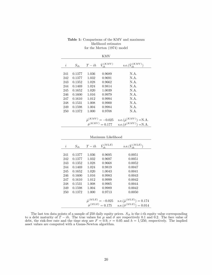
The top panel of Table 1 provides an example of the KMV estimation using a simulated sample

of daily equity values using V0 = 1, µ = 0.1, σ = 0.2, T = 2, F = 0.9, r = 0.05, n = 250

and h = 1/250. For this example, the initial value for the volatility is set to σ̂(0) = 0.2 and the

convergence criteria is 1 × 10−6, that is, we stop the iteration when the difference between twosuccessive estimation of σ is less than 1 × 10−6. The parameter values corresponding to the finaliteration are presented in this table along with the implied asset values for the last 10 data points.

The KMV algorithm converges to µ̂ = −0.025 and σ̂ = 0.177. The final implied asset value for

the last data point, V250h, is 0.9708. This implied asset value along with µ̂ and σ̂ can be used to

compute, for instance, a default probability estimate corresponding to the last data point, which

turns out to be 0.420.

2.3 The transformed-data maximum likelihood estimation

The estimation problem associated with unobserved asset values can be naturally cast as a transformed-

data maximum likelihood estimation (MLE) problem. Such an approach was first developed in

Duan (1994). The obvious advantages are that (1) the resulting estimators are known to be statis-

tically efficient in large samples, and (2) sampling distributions are readily available for computing

confidence intervals or for testing hypotheses.

We denote the log-likelihood function of the observed data set under a specified model as

L(θ; data) where θ is the set of unknown parameters under the model. The MLE is to find the

value of θ at which the data set has the highest likelihood of occurrence. Under Merton’s (1974)

model and assuming that one could directly observe the firm’s asset values {V0, Vh, · · · , Vnh}, the

6

log-likelihood function could be written as :

LV (µ, σ;V0, Vh, · · · , Vnh) = −n2ln¡2πσ2h

¢− 12

nXk=1

³Rk −

³µ− σ2

2

´h´2

σ2h−

nXk=1

lnVkh (6)

where Rk = ln¡Vkh/V(k−1)h

¢.2 This log-likelihood is a result of assuming the geometric Brownian

motion for the asset value dynamic. If the firm had undergone one or more times of refinancing,

survivorship becomes an important issue. Duan, et al (2003) offers the survivorship adjustment for

Merton’s (1974) model.

We, however, do not observe the firm’s asset values. Typically, the firm’s equity values are

available. Recognizing that Merton’s (1974) model implicitly provides a one-to-one smooth rela-

tionship between the equity and asset values, one can invoke the standard result on differentiable

transformations to derive the log-likelihood function solely based on the observed equity data. If

we denote the density of the asset value as f(V ), the density associated with the equity will be

given by f(V )/¯̄̄∂g(V ;σ)∂V

¯̄̄. Applying this knowledge yields the following log-likelihood function on

the observed equity data :

LS (µ, σ;S0, Sh, · · · , Snh) = LV³µ, σ; V̂0(σ), V̂h(σ), · · · , V̂nh(σ)

´−

nXk=1

ln³Φ³d̂kh(σ)

´´(7)

where V̂kh(σ) = g−1 (Skh;σ) and d̂kh(σ) =ln(V̂kh(σ)/F)+

³r+σ2

2

´(T−kh)

σ√T−kh . Note that the inversion

does not require µ because the equity pricing equation in (5) is not a function of this parameter.

Moreover, ∂g(Vkh;σ)∂Vkh

= Φ (dkh).

One can easily find the ML estimates for µ and σ by numerically maximizing the function in

(7). Moreover, one can rely on the ML inference to compute approximate confidence intervals for

the estimated parameters — µ̂ and σ̂ — and other quantities of interest such as the implied asset

value V̂nh(σ̂), the risky bond price D̂nh(V̂nh(σ̂), σ̂) and the default probability P̂nh(V̂nh(σ̂), µ̂, σ̂).

Appendix A provides further discussion on inference.

We take the same equity data sample as in the case of the KMV estimation to compute the ML

estimates and report the final results in the bottom panel of Table 1. We have used a convergence

criterion of 1 × 10−6 and the initial parameter values of 0.2 for σ and 0.1 for µ to obtain the ML2The term −Pn

k=1 lnVkh could be ignored at the optimization stage if the firm’s asset values were directlyobservable since it would simply amount to an irrelevant constant. We must keep this term in order to later dealwith the fact that the asset value is not observable. This point was made in Duan (2000).

7

estimates: µ̂ = −0.025 and σ̂ = 0.175 along with their standard errors. The ML estimates are thenused to compute the implied asset values and their corresponding standard errors. The results for

the final implied asset values and standard errors of the last ten data points are given in the table.

Comparing the two panels, it is clear that the KMV and ML estimates for µ and σ are very

close. This result is not a fluke, and its theoretical reason will be given in the next subsection. The

final implied asset values are also very close.3 In contrast to the KMV approach, the MLE method

can readily generate standard errors, which are also reported in the table.

2.4 Equivalence

We now proceed to show theoretically that the KMV estimates are the ML estimates for Merton’s

(1974) model. Our theoretical argument is based on a statistical tool known as the EM algorithm.

This algorithm long existed in the statistical literature in different forms. Dempster et al (1977)

were the first to coin the term and provided a comprehensive treatment of the method. The

EM algorithm is essentially an alternative way of obtaining the ML estimate for the incomplete

data model, where incomplete data refers to the situation that the model contains some random

variable(s) without corresponding observations.

The EM algorithm involves two steps - expectation and maximization - and hence its name.

One first writes down the log-likelihood function by assuming the complete data. The expectation

of the complete-data log-likelihood function is then evaluated, conditional on the observed data

and some assumed parameter values. This completes the expectation step. In the maximization

step, one finds the new parameter values that maximize the conditionally expected complete-data

log-likelihood function. The updated parameter values are then used to repeat the E and M steps

until convergence is achieved. Interestingly, the EM algorithm will converge to the ML parameter

estimates based on the incomplete data.4 Although the EM algorithm is a very powerful tool, its

practicality diminishes markedly when the conditional expectation cannot be analytically evaluated

and/or the maximization step cannot be solved analytically.

We argue that the KMV method is an EM algorithm in the context of Merton’s (1974) model.

3Although these two approaches can be shown to converge to the same values theoretically, numerical differencescan be expected because numerical approximations used in defining the equity pricing function and in differentiationsfor the optimization purpose; for example, the standard polynomial approximation of the standard normal distributionfunction used in our program has an accuracy up to the sixth decimal place.

4The EM algorithm is not immune to the usual multi-modal problem associated with numerical optimization. Inother words, the limit point of the EM algorithm may be a local maximum, just like the typical ML estimation.

8

A formal proof is given in Appendix B. We provide here a sketch of that proof. In the E-step, one

first forms the log-likelihood function associated with the unobserved asset values, i.e., equation

(6), which can be viewed as the complete-data log-likelihood using the jargon of the EM algorithm.

We then compute its expected value conditional on the observed equity values and some values of µ

and σ. Actually, we do not need the value of µ in the E-step because the implied asset value is not

a function of µ. Since the relationship between the unobserved asset value and the observed equity

value is one-to-one for a given value of σ, this conditional expectation becomes trivial. In fact, it

amounts to the log-likelihood function based on the firm’s asset values as if they were observed at

those implied asset values. The parameter values that maximize this function are those given in

Step 2 of the KMV method, which in turn means that the M-step will yield the same estimates

for µ and σ as in a KMV update. In short, the KMV method is a degenerate EM algorithm with

degeneracy occurring in the E-step.

3 General non-equivalence between the KMV and MLE methods

Merton’s (1974) model contains only two unknown parameters and both of which pertain only to the

dynamic of the firm’s asset value. In general, structural models may contain unknown parameters

specific to capital structure. There are numerous examples in the literature. In this section, we

focus on the model of Brockman and Turtle (2003) and use it to make an important point on general

non-equivalence between the KMV and MLE methods. The Brockman and Turtle (2003) model

assumes the same asset value dynamic as that of Merton’s (1974). However, unlike Merton’s (1974)

model, the firm can default at any time prior to the maturity of its debt. A default occurs when the

asset value crosses a financial distress level, denoted by K, which can be interpreted as breaching,

for example, the debt covenants. The firms’ equity can be likened to a European down-and-out call

option with the financial distress level serving as the barrier. Since the financial distress level is

unknown, their model has three unknown parameters: µ, σ and K. The first two are specific to the

asset value dynamic whereas K is related to the capital structure of the firm. The equity pricing

formula of this model can be written generically as St = g(Vt;σ,K), a function of the firm’s asset

value that depends on two unknown parameters. Its specific expression is given in Appendix C.

Brockman and Turtle (2003) conducted an empirical study using a market value proxy for the

unobserved asset value of the firm. They concluded that the companies in their large sample of

9

industrial firms face high financial distress levels (relative to their book values of liabilities). Wong

and Choi (2004), however, argued that the high financial distress level is induced by the use of

the market value proxy for it is upward biased. They then adopted the transformed-data MLE

approach of Duan (1994) to derive the likelihood function for the Brockman and Turtle (2003)

model. They proceeded to empirically estimate the model for a large sample of firms and yielded

estimates of the financial distress level that are much lower than those based on the market value

proxy.

Our purpose here is to use the Brockman and Turtle (2003) model to illustrate the limitation

of the KMV method. In short, we will show that the KMV method cannot estimate the capital

structure parameter. In addition, the KMV method does not deal with the survivorship issue that

is inherent in the estimation of a structural model like Brockman and Turtle (2003). In contrast,

the transformed-data MLE approach can handle both.

It is fairly easy to see why the KMV method cannot generate a meaningful estimate for the

financial distress levelK. Starting with σ̂(0) and K̂(0), one can invert the time series of equity values

to obtain their corresponding implied asset values; that is, V̂ih(σ̂(0), K̂(0)) = g−1(Sih; σ̂(0), K̂(0)) with

g defined in Appendix C. Then, apply Step 2 of the KMV method to obtain the updated values:

σ̂(1) and µ̂(1). The implied asset values do not, however, provide a mechanism for updating K.

Thus, K̂(1) = K̂(0). In short, K will remain at its arbitrary initial value even though µ and σ have

been updated.

Again we can use the EM algorithm to better understand the nature of the KMV method in

this context. Similar to Merton’s model (1974), one first derives the complete-data log-likelihood

function, which is expected to be different from equation (6). This is simply due to the fact that if

a firm has survived the sample period, it means that the firm’s asset values must have stayed above

the financial distress level for the entire period. Let Di ≡©inft∈[0,ih] Vt > K

ªbe the event that no

default occurred up to time ih. The complete-data log-likelihood function of the Brockman and

Turtle (2003) model can be written as

LVBT (µ, σ,K;V0, Vh, · · · , Vnh|Dn)

= LV (µ, σ;V0, Vh, · · · , Vnh) + lnP (Dn |V0, Vh, · · · , Vnh;σ,K )− lnP (Dn;µ, σ,K) (8)

The third term in the above expression can be analytically derived using the well-known probability

of the Brownian motion infimum. The second term is more complicated and requires the knowledge

10

of the joint probability for the Brownian motion and its infimum. It turns out that the conditional

survival probability is not a function of µ. The exact expressions for these two terms are given in

Appendix C.

The expected value of the complete-data log-likelihood function conditional on the observed

equity values and some parameter values can thus be computed. The result is the log-likelihood

function with the firm’s asset values being fixed at the implied asset values, say, in the m-th itera-

tion. Thus, this function can be written as LVBT

³µ, σ,K; V̂0(σ̂

(m), K̂(m)), · · · , V̂nh(σ̂(m), K̂(m))|Dn

´.

Obviously, maximizing this function will lead to updated estimates — µ̂(m+1), σ̂(m+1) and K̂(m+1) —

that are different from those produced by the KMV updating step. It is now clear that the KMV

method is not an EM algorithm for the Brockman and Turtle (2003) model. Thus, there is no

reason to expect that the KMV method should yield the ML estimates.

The above discussion provides an EM algorithm for estimating the Brockman and Turtle (2003)

model even though the result produced by the EM algorithm no longer coincides with that from

the KMV method. The M-step is simply to find µ̂(m+1), σ̂(m+1) and K̂(m+1) that maximize

LVBT

³µ, σ,K; V̂0(σ̂

(m), K̂(m)), · · · , V̂nh(σ̂(m), K̂(m))|Dn

´. Conceptually, this EM algorithm will con-

verge to the maximum likelihood estimates. Operationally, however, it is not an attractive approach

mainly because the M-step does not have an analytical solution. The numerical implementation of

this EM algorithm thus becomes a two-layer loop where the M-step constitutes the inner loop.

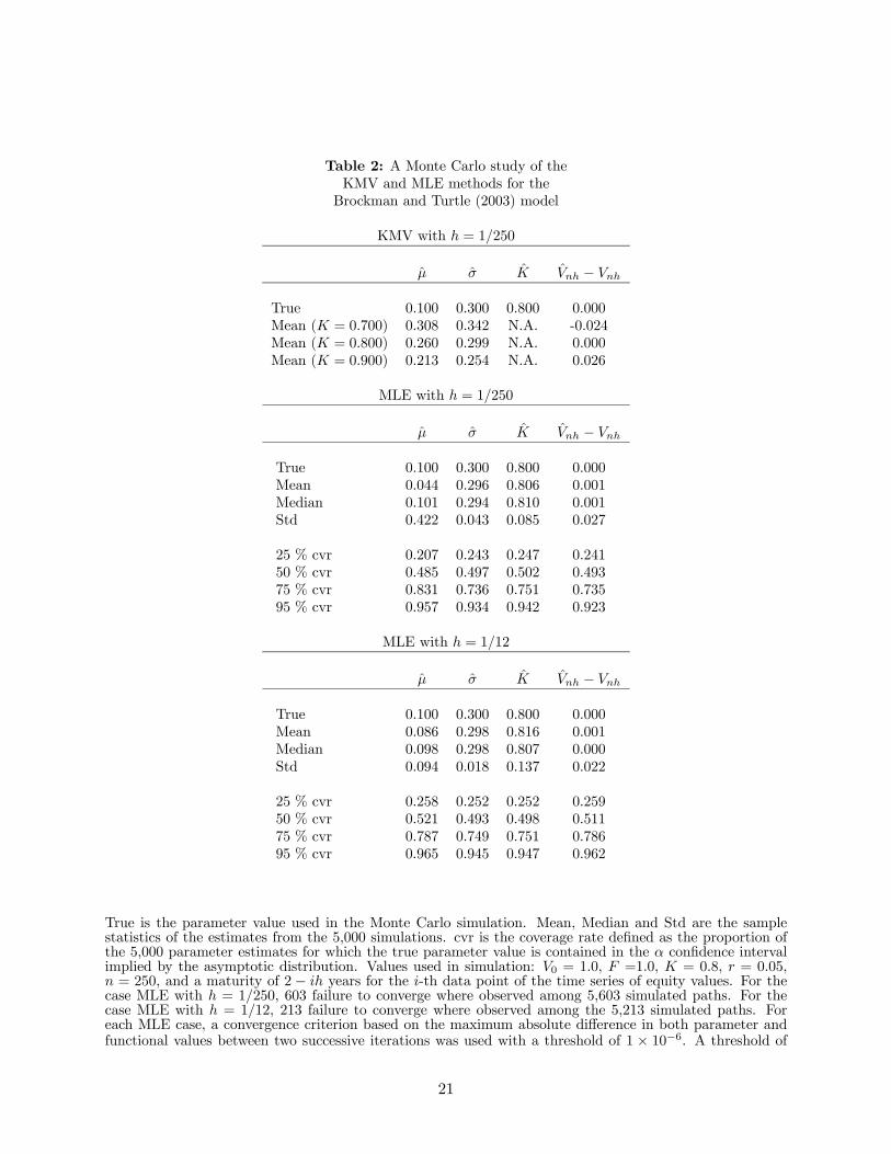
We now use a simulation study to numerically examine the non-equivalence between the KMV

and maximum likelihood estimator. Doing so requires the derivation of the log-likelihood function

based on the observed equity values under the Brockman and Turtle (2003) model. Its derivation

is provided in Appendix C. As discussed earlier, the MLE for this model has been developed in

Wong and Choi (2004).5

We use the following parameter values to perform the simulation: r = 0.05, µ = 0.1, σ =

0.3, V0 = 1.0, F = 1.0,K = 0.8, h = 1/250, n = 250 and a maturity of (2 − jh) years for the j-th

data point of the time series. Since the Brockman and Turtle (2003) model is based on continuous

monitoring of financial distress, the simulation of the firm’s asset values is conducted by dividing

one day into 50 subintervals. If a simulated sample breaches the barrier at any one of the 12, 500

monitoring points, the sample is discarded. We then compute the 251 corresponding daily equity

values for any kept sample, and then act as if the firm’s asset values were not available. In short,

5 It is our belief that Wong and Choi’s (2004) log-likelihood function contains minor errors.

11

we try to mimic a daily sample of observed equity values of a survived firm.

In order to implement the KMV method, one must commit to a specific value of K. The top

panel of Table 2 reports the average values of the KMV estimates for µ and σ from 5, 000 simulated

samples. In all cases, the initial σ is set to 0.3. When the true value of K is used, i.e., K = 0.8, the

estimated σ appears to be unbiased. It is not the case for µ, however, and in fact it is substantially

upward biased with an average of more than twice the true value. This result is consistent with

the survivorship analysis presented in Duan, et al (2003) for Merton’s (1974) model. They show

that failing to adjust for survivorship will result in an upward biased estimate for µ but not for σ.

When an incorrect financial distress level is assumed, i.e., K = 0.7 or 0.9, the estimate either for µ

or σ is of poor quality, a result that is hardly surprising.

The results based on the transformed-data MLE approach on the same 5, 000 simulated samples

are reported in the second panel of Table 2.6 The results show that the average parameter estimates

for σ, K and Vnh are centered around the correct values. Furthermore, the coverage rates suggest

that the actual distributions are reasonably approximated by the asymptotic normal distributions.7

However, there exists a downward bias for the drift parameter µ for the sample size of 250 daily

observations. It is well known in the literature that the drift parameter can only be estimated

accurately using a long time span of data. In this transformed-data MLE setting with one-year

worth of daily data, it is hardly surprising to experience the same difficulty. The bias is, however,

of a much smaller magnitude than the upward bias observed with the KMV approach. To gain a

better understanding of the bias, we have performed an additional Monte Carlo experiment with

the results being reported in the third panel of Table 2. The parameters of this experiment are

identical to those of the second panel except that h is set equal to 1/12. 8 The bias in the estimated

µ clearly becomes smaller as reflected in the fact that the mean is much closer to the true parameter

value.6As it is often the case in Monte Carlo experiments that involve non-linear optimization, convergence failure may

occur in some fraction of cases. Whenever that happens, we add new replications in order to have 5, 000 simulatedsamples with proper convergence. The numbers of failed convergence are reported in the tables.

7A coverage rate represents the proportion of the 5, 000 estimates for which the true parameter value is containedin the α confidence interval implied by the corresponding asymptotic normal distribution.

8The simulation of the firm’s asset values is conducted by dividing each month into 1, 050 subintervals.

12

4 Conclusion

The implementation of structural credit risk models requires estimates for asset values and model

parameters. We have provided an analysis on the statistical properties of Moody’s KMV method

for Merton’s (1974) model. We have shown theoretically that the KMV estimates are identical to

the ML estimates when Merton’s (1974) model is employed. This theoretical result relies on casting

the KMV method as an EM algorithm. Even under Merton’s (1974) model, the KMV method is not

equivalent to the MLE method, because the former is limited to generating point estimates whereas

the latter has accompanying distributional information ideal for conducting statistical inference.

For structural models containing unknown capital structure parameter(s), for example, Brockman

and Turtle (2003), we have shown that the KMV method does not generate suitable estimates and

fails to address an inherent survivorship issue.

The KMV method is nevertheless an intuitive and numerically efficient way of obtaining point

estimates under Merton’s (1974) model. Our linking it to the EM algorithm actually opens up

ways to modify the KMV method for different structural models. However, such modified schemes

are likely to be numerically inefficient because the practicality of the EM algorithm largely rests on

one’s ability to obtain the analytical solutions in both the E and M steps. For structural models in

general, the E step will remain to be a degenerate expectation operation but the M step is unlikely

to have an analytical solution.

A Maximum likelihood inference

Inference is an important part of statistical analysis. The ML inference for the structural credit risk

model can be easily implemented using numerical differentiation. For a sufficiently large sample

size n, the distribution of the maximum likelihood parameter estimates, stacked in a column vector

θ̂, can be well approximated by the following normal distribution :

θ̂ ≈ N¡θ0,H

−1n

¢where θ0 denotes the true parameter value vector and Hn is the negative of the second derivative

matrix of the log-likelihood function with respect to θ; that is,

Hn = −∂L(θ; data)∂θ∂θ0

¯̄̄̄θ = θ̂

13

For any differentiable transformation of the ML estimates, f(θ̂), the standard statistical result

implies that

f(θ̂) ≈ N

Ãf(θ0),

"∂f(θ̂)

∂θ

#0H−1n

∂f(θ̂)

∂θ

!

where ∂f(θ̂)∂θ is a column vector of the first partial derivatives of the function with respect to the

elements of θ being evaluated at θ̂. This standard result was, for example, utilized in Lo (1986) in

the context of testing the derivative pricing model.

In the context of Merton’s (1974) model, θ = (µ, σ)0. For the implied asset value, one needs to

recognize that it is a differentiable function of σ̂. The specific analytical result for the distribution

of the implied asset value is available in equation (4.7) of Duan (1994). The expressions for the

risky bond and default probability can be derived in a way similar to the deposit insurance value

in equation (4.8) of Duan (1994). The derivation requires one to recognize that both risky bond

price and default probability are direct as well as indirect functions of the parameter(s) with the

indirectness through the implied asset value.

B The KMV method is an EM algorithm

We now describe the EM algorithm for estimating Merton’s (1974) model in the framework laid

out in Dempster, et al (1977). By assuming that both the firm’s asset and equity values could be

observed, we can express the log-likelihood function of the complete data by

L (µ, σ;V0, Vh, · · · , Vnh, S0, Sh, · · · , Snh) = LV (µ, σ;V0, Vh, · · · , Vnh) +nXi=0

ln1{Sih=g(Vih;σ0)}

where 1{•} is the indicator function. The indicator function appears because non-zero likelihood

only occurs at the points where the equity and asset values satisfy the equity pricing equation

evaluated at the unknown true volatility parameter σ0. For the EM algorithm, we can in fact drop

the sum involving the indicator function, a point that will become clear later in the E step.

14

E-step: Compute

EhL (µ, σ;V0, Vh, · · · , Vnh, S0, Sh, · · · , Snh)

¯̄̄S0, Sh, · · · , Snh, µ̂(m), σ̂(m)

i= LV

³µ, σ; V̂0(σ̂

(m)), V̂h(σ̂(m)), · · · , V̂nh(σ̂(m))

´+

nXi=0

ln1{Sih=g(V̂ih(σ̂(m));σ̂(m))}

= LV³µ, σ; V̂0(σ̂

(m)), V̂h(σ̂(m)), · · · , V̂nh(σ̂(m))

´= −n

2ln¡2πσ2h

¢− 12

nXk=1

³R̂(m)k −

³µ− σ2

2

´h´2

σ2h−

nXk=1

ln V̂kh(σ̂(m))

where R̂(m)k = ln³V̂kh(σ̂

(m))/V̂(k−1)h(σ̂(m))´and V̂kh(σ̂

(m)) = g−1(Skh; σ̂(m)).

M-step: Maximize the conditional log-likelihood function obtained in the E-step to yield³σ̂(m+1)

´2=1

nh

nXk=1

³R̂(m)k − R̄(m)

´2µ̂(m+1) =

1

hR̄(m) +

1

2

³σ̂(m+1)

´2where R̄(m) = 1

n

Pnk=1 R̂

(m)k .

It is now clear that the KMV method as described in the text is indeed an EM algorithm. It

is easy to verify LV³µ, σ; V̂0(σ̂

(m)), V̂h(σ̂(m)), · · · , V̂nh(σ̂(m))

´satisfies the conditions in Theorem 4

of Dempster, et al (1977) so that the KMV method for Merton’s model yield the ML estimates for

µ and σ.

C The Brockman and Turtle (2003) model and the correspondinglikelihood function

In Brockman and Turtle (2003), the firm’s equity is viewed as a European down-and-out call option

with the strike price F , barrier K and maturity T . Thus, the equity pricing equation is:

St = VtΦ(at)− Fe−r(T−t)Φ³at − σ

√T − t

´− Vt (K/Vt)

2η Φ (bt)

+Fe−r(T−t) (K/Vt)2η−2Φ

³bt − σ

√T − t

´

15

where Φ (•) is the standard normal distribution function,

at =ln Vt

max(F,K) +³r + σ2

2

´(T − t)

σ√T − t

bt = at −2 ln Vt

K

σ√T − t

η =r

σ2+1

2.

Note that there is a rebate rate in Brockman and Turtle’s (2003) original formula. In their imple-

mentation, however, the rebate rate was set to zero. The formula above reflects the special case of

a zero rebate rate.

Denote the above equity pricing equation by g(Vt;σ,K) to reflect the fact that it is a function

of the firm’s asset value and depends on two unknown parameters. We can apply the transformed-

data MLE method of Duan (1994) to obtain the log-likelihood function of a discretely sampled

equity values on a firm that survives the entire sample period. It turns out to be the log-likelihood

function of the firm’s asset value conditional on survival (equation (8)) evaluated at the implied

asset values plus a term related to the Jacobian of the transformation. Thus,

LSBT (µ, σ,K;S0, Sh, ..., Snh|Dn)

= LVBT

³µ, σ,K; V̂0(σ,K), V̂h(σ,K), · · · , V̂nh(σ,K)|Dn

´−

nXj=1

ln

¯̄̄̄¯∂g(V̂jh(σ,K);σ,K)∂Vjh

¯̄̄̄¯

= LV³µ, σ; V̂0(σ,K), V̂h(σ,K), · · · , V̂nh(σ,K)

´+ lnP

³Dn|V̂0(σ,K), V̂h(σ,K), · · · , V̂nh(σ,K);σ,K

´− lnP (Dn;µ, σ,K)−

nXj=1

ln

¯̄̄̄¯∂g(V̂jh(σ,K);σ,K)∂Vjh

¯̄̄̄¯ .

where the first derivative of the equity value with respect to the asset value can be derived to be

∂g(Vt;σ,K)

∂Vt= Φ (at) +

1

σ√T − t

"φ (at)− Fe−r(T−t)

Vtφ³at − σ

√T − t

´#

+

µK

Vt

¶2η−1 "(2η − 1) K

VtΦ (bt) +

Fe−r(T−t)

K(2− 2η)Φ

³bt − σ

√T − t

´#

+1

σ√T − t

µK

Vt

¶2η−1 "KVtφ (bt)− Fe−r(T−t)

Kφ³bt − σ

√T − t

´#

with φ(·) representing the standard normal density function.

16

It remains to derive the expressions for P (Dn;µ, σ,K) and P (Dn|V0, Vh, · · · , Vnh;σ,K). Firstrecall the following result for the infimum of a Brownian motion with drift:

P

½inf0≤s≤t

Ws + as > y

¾=

⎧⎪⎨⎪⎩Φ³at−y√

t

´− exp(2ay)Φ

³at+y√

t

´if y ≤ 0

0 otherwise

Thus,

P (Dn;µ, σ,K) = Φ

Ã(µ− σ2

2 )nh− ln KV0√

nhσ

!− exp

Ã2(µ− σ2

2 )

σ2ln

K

V0

!Φ

Ã(µ− σ2

2 )nh+ lnKV0√

nhσ

!.

The joint distribution of the Brownian motion with drift and its infimum is known to be

P

½inf0≤s≤t

Ws + as ≤ y & Wt + at ≥ x

¾= exp(2ay)Φ

µ2y − x+ at√

t

¶for y ≤ min(x, 0).

As a result, the distribution of the infimum conditional on two end points becomes

P

½inf0≤s≤t

Ws + as ≤ y

¯̄̄̄W0 = 0,Wt = b

¾=exp(2ay)φ

³2y−b√

t

´φ³

b√t

´for y ≤ min(b+ at, 0). This result can be used to characterize the distribution of the infimum up

to time ih while conditioning on V(i−1)h, Vih and the infimum up to time (i− 1)h. Hence,

Hi(v) ≡ P

½inf

0≤s≤ihVs ≤ v

¯̄̄̄V(i−1)h, Vih, inf

0≤s≤(i−1)hVs

¾= 1{inf0≤s≤(i−1)h Vs≤v} + 1{inf0≤s≤(i−1)h Vs>v}P

½inf

(i−1)h≤s≤ihVs ≤ v|V(i−1)h, Vih

¾Let W ∗

s∗ ≡Ws−W(i−1)h where s∗ ≡ s− (i− 1)h for s ≥ (i− 1)h. For v < min(V(i−1)h, Vih), we cancompute

P

½inf

(i−1)h≤s≤ihVs ≤ v

¯̄̄̄V(i−1)h, Vih

¾= P

½inf

0≤s∗≤hW ∗

s +µ− σ2/2

σs∗ ≤ 1

σln

v

V(i−1)h

¯̄̄̄W ∗0 = 0,W

∗h =

1

σln

VihV(i−1)h

− (µ− σ2/2)h

σ

¾

=exp

³2(µ−σ2/2)

σ2ln v

V(i−1)h

´φ³ln(v/V(i−1)h)+ln(v/Vih)+(µ−σ2/2)h

σ√h

´φ³ln(Vih/V(i−1)h)−(µ−σ2/2)h

σ√h

´= exp

⎛⎝2 ln Vihv ln

vV(i−1)h

σ2h

⎞⎠ .

17

For either v ≥ V(i−1)h or v ≥ Vih, it is obvious that P©inf(i−1)h≤s≤ih Vs ≤ v

¯̄V(i−1)h, Vih

ª= 1.

Thus, for v < min(V(i−1)h, Vih, inf0≤s≤(i−1)h Vs),

Hi(v) = exp

⎛⎝2 ln Vihv ln v

V(i−1)h

σ2h

⎞⎠ .

Otherwise, Hi(v) = 1.

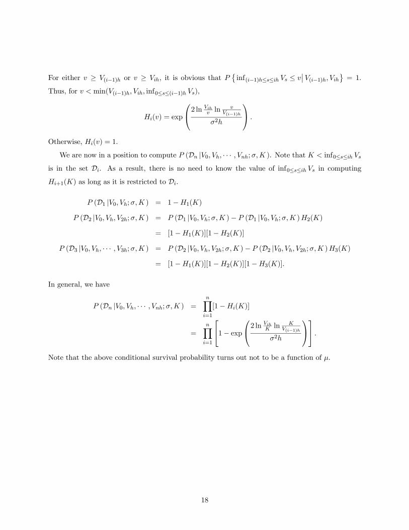
We are now in a position to compute P (Dn |V0, Vh, · · · , Vnh;σ,K ). Note that K < inf0≤s≤ih Vs

is in the set Di. As a result, there is no need to know the value of inf0≤s≤ih Vs in computing

Hi+1(K) as long as it is restricted to Di.

P (D1 |V0, Vh;σ,K ) = 1−H1(K)

P (D2 |V0, Vh, V2h;σ,K ) = P (D1 |V0, Vh;σ,K )− P (D1 |V0, Vh;σ,K )H2(K)

= [1−H1(K)][1−H2(K)]

P (D3 |V0, Vh, · · · , V3h;σ,K ) = P (D2 |V0, Vh, V2h;σ,K )− P (D2 |V0, Vh, V2h;σ,K )H3(K)

= [1−H1(K)][1−H2(K)][1−H3(K)].

In general, we have

P (Dn |V0, Vh, · · · , Vnh;σ,K ) =nYi=1

[1−Hi(K)]

=nYi=1

⎡⎣1− exp⎛⎝2 ln Vih

K ln KV(i−1)h

σ2h

⎞⎠⎤⎦ .Note that the above conditional survival probability turns out not to be a function of µ.

18

References[1] Brockman, P. and H. Turtle, 2003, A Barrier Option Framework for Corporate Security Val-

uation, Journal of Financial Economics 67, 511-529.

[2] Bharath, T. and T. Shumway, 2004, Forecasting Default with the KMV-Merton Model, Uni-versity of Michigan working paper.

[3] Cao, C., Simin, T. and J. Zhao, 2005, Do Growth Options Explain the Trend in IdiosyncraticRisk?, Pensylvania State working paper.

[4] Crosbie, P. and J. Bohn, 2003, Modeling Default Risk, Moody’s KMV technical document.

[5] Dempster, A., Laird, N., and D. Rubin, 1977, Maximum-likelihood from Incomplete Data Viathe EM Algorithm, Journal of the Royal Statistical Society B 39, 1-38.

[6] Duan, J.C., 1994, Maximum Likelihood Estimation Using Price Data of the Derivative Con-tract, Mathematical Finance 4, 155-167.

[7] Duan, J.C., 2000, Correction: Maximum Likelihood Estimation Using Price Data of the Deriv-ative Contract, Mathematical Finance 10, 461-462.

[8] Duan, J.C., G. Gauthier, J.G. Simonato and S. Zaanoun, 2003, Estimating Merton’s Model byMaximum Likelihood with Survivorship Consideration, University of Toronto working paper.

[9] Eom, Y., J. Helwege and J. Huang, 2004, Structural Models of Corporate Bond Pricing: AnEmpirical Analysis, Review of Financial Studies 17, 499-544.

[10] Ericsson, J. and J. Reneby, 2003, Estimating Structural Bond Pricing Models, to appear inJournal of Business.

[11] Jarrow, R. and S. Turnbull, 2000, The Intersection of Market and Credit Risk, Journal ofBanking and Finance 24, 271-299.

[12] Jones, E., Mason, S. and E. Rosenfeld, 1984, Contingent Claims Analysis of Corporate CapitalStructures: An Empirical Investigation, Journal of Finance 39, 611-627.

[13] Lo, A., 1986, Statistical Tests of Contingent-Claims Asset-Pricing Models - A New Methodol-ogy, Journal of Financial Economics 17, 143-173.

[14] Merton, R., 1974, On the Pricing of Corporate Debt: the Risk Structure of Interest Rates,Journal of Finance 28, 449-470.

[15] Ronn, E.I. and A.K. Verma, 1986, Pricing Risk-Adjusted Deposit Insurance: An Option-BasedModel, Journal of Finance 41, 871-895.

[16] Vassalou, M. and Y. Xing, 2004, Default Risk in Equity Returns, Journal of Finance 59,831-68.

[17] Wong, H. and T. Choi, 2004, The Impact of Default Barrier on the Market Value of Firm’sAsset, Chinese University of Hong Kong working paper.

19

Table 1: Comparisons of the KMV and maximumlikelihood estimates

for the Merton (1974) model

KMV

i Sih T − ih V̂(KMV )ih s.e.(V̂ (KMV )

ih )

241 0.1377 1.036 0.9689 N.A.242 0.1377 1.032 0.9691 N.A.243 0.1352 1.028 0.9662 N.A.244 0.1469 1.024 0.9814 N.A.245 0.1652 1.020 1.0039 N.A.246 0.1600 1.016 0.9979 N.A.247 0.1610 1.012 0.9994 N.A.248 0.1531 1.008 0.9900 N.A.249 0.1598 1.004 0.9984 N.A.250 0.1372 1.000 0.9708 N.A.

µ̂(KMV ) = −0.025 s.e.(µ̂(KMV )) =N.A.σ̂(KMV ) = 0.177 s.e.(σ̂(KMV )) =N.A.

Maximum Likelihood

i Sih T − ih V̂(MLE)ih s.e.(V̂ (MLE)

ih )

241 0.1377 1.036 0.9695 0.0051242 0.1377 1.032 0.9697 0.0051243 0.1352 1.028 0.9668 0.0052244 0.1469 1.024 0.9819 0.0047245 0.1652 1.020 1.0043 0.0041246 0.1600 1.016 0.9983 0.0043247 0.1610 1.012 0.9999 0.0042248 0.1531 1.008 0.9905 0.0044249 0.1598 1.004 0.9989 0.0042250 0.1372 1.000 0.9713 0.0050

µ̂(MLE) = −0.025 s.e.(µ̂(MLE)) = 0.174

σ̂(MLE) = 0.175 s.e.(σ̂(MLE)) = 0.014

The last ten data points of a sample of 250 daily equity prices. Sih is the i-th equity value correspondingto a debt maturity of T − ih. The true values for µ and σ are respectively 0.1 and 0.2. The face value ofdebt, the risk-free rate and the time step are F = 0.9, r = 0.05 and h = 1/250, respectively. The impliedasset values are computed with a Gauss-Newton algorithm.

20

Table 2: A Monte Carlo study of theKMV and MLE methods for theBrockman and Turtle (2003) model

KMV with h = 1/250

µ̂ σ̂ K̂ V̂nh − Vnh

True 0.100 0.300 0.800 0.000Mean (K = 0.700) 0.308 0.342 N.A. -0.024Mean (K = 0.800) 0.260 0.299 N.A. 0.000Mean (K = 0.900) 0.213 0.254 N.A. 0.026

MLE with h = 1/250

µ̂ σ̂ K̂ V̂nh − Vnh

True 0.100 0.300 0.800 0.000Mean 0.044 0.296 0.806 0.001Median 0.101 0.294 0.810 0.001Std 0.422 0.043 0.085 0.027

25 % cvr 0.207 0.243 0.247 0.24150 % cvr 0.485 0.497 0.502 0.49375 % cvr 0.831 0.736 0.751 0.73595 % cvr 0.957 0.934 0.942 0.923

MLE with h = 1/12

µ̂ σ̂ K̂ V̂nh − Vnh

True 0.100 0.300 0.800 0.000Mean 0.086 0.298 0.816 0.001Median 0.098 0.298 0.807 0.000Std 0.094 0.018 0.137 0.022

25 % cvr 0.258 0.252 0.252 0.25950 % cvr 0.521 0.493 0.498 0.51175 % cvr 0.787 0.749 0.751 0.78695 % cvr 0.965 0.945 0.947 0.962

True is the parameter value used in the Monte Carlo simulation. Mean, Median and Std are the samplestatistics of the estimates from the 5,000 simulations. cvr is the coverage rate defined as the proportion ofthe 5,000 parameter estimates for which the true parameter value is contained in the α confidence intervalimplied by the asymptotic distribution. Values used in simulation: V0 = 1.0, F =1.0, K = 0.8, r = 0.05,n = 250, and a maturity of 2 − ih years for the i-th data point of the time series of equity values. For thecase MLE with h = 1/250, 603 failure to converge where observed among 5,603 simulated paths. For thecase MLE with h = 1/12, 213 failure to converge where observed among the 5,213 simulated paths. Foreach MLE case, a convergence criterion based on the maximum absolute difference in both parameter andfunctional values between two successive iterations was used with a threshold of 1 × 10−6. A threshold of

21

1× 10−4 for the gradient norm was also used to determine the validity of a solution obtained with the hillclimbing algorithm.

22