On the essentiality of E-money - Home | Victoria University · PDF file ·...

WORKING PAPERS IN ECONOMICS AND FINANCE

School of Economics and Finance | Victoria Business School | www.victoria.ac.nz/sef

On the essentiality of E-money

Jonathan Chiu and Tsz-Nga Wong

SEF WORKING PAPER 14/2016

The Working Paper series is published by the School of Economics and Finance to provide staff and research students the opportunity to expose their research to a wider audience. The opinions and views expressed in these papers are not necessarily reflective of views held by the school. Comments and feedback from readers would be welcomed by the author(s). Further enquiries to:

The Administrator School of Economics and Finance Victoria University of Wellington P O Box 600 Wellington 6140 New Zealand Phone: +64 4 463 5353 Email: [email protected]

Working Paper 14/2016

ISSN 2230-259X (Print)

ISSN 2230-2603 (Online)

mailto:[email protected]

On the Essentiality of E-money∗

Jonathan ChiuVictoria University of Wellington

Tsz-Nga WongBank of Canada

July 2016

Abstract

Recent years have witnessed the advances of e-money systems such as Bitcoin,

PayPal and various forms of stored-value cards. This paper adopts a mechanism

design approach to identify some essential features of different payment systems

that implement the optimal resource allocation. We find that, compared to

cash, e-money technologies allowing limited participation, limited transferability

and non-zero-sum transfers can help mitigate fundamental frictions and enhance

social welfare, if they satisfy conditions in terms of parameters such as trade fre-

quency and bargaining powers. An optimally designed e-money system exhibits

realistic arrangements including non-linear pricing, cross-subsidization and posi-

tive interchange fees even when the technologies incur no costs. Regulations such

as a cap on interchange fees (à la the Dodd-Frank Act) can distort the optimal

mechanism and reduce welfare.

Keywords: money, electronic money, mechanism design, search and matching,

effi ciency.

JEL Codes: E, E4, E42, E5, E58, L5, L51

∗We are grateful to Charlie Kahn, Will Roberds, Steve Williamson and Shengxing Zhang as thediscussants for this paper. We have benefited from the comments and suggestions of members of theBank of Canada E-money Working Group, Ben Fung, Scott Hendry, Tai-Wei Hu, Miguel Molico, PedroGomis-Porqueras, Guillaume Rocheteau, Marc Rysman, Daniel Sanches, Oz Shy, Robert Townsend,Neil Wallace, Zhu Wang, Warren Weber, Randy Wright and seminar participants at the Universityof Wisconsin at Madison, FRB of Philadelphia, FRB of Chicago, AMES 2014, CEA-CMSG 2014,Singapore Management University, Chinese University of Hong Kong, Bank of Canada and Economicsof Payment VII Conference at Boston Fed. The views expressed here do not necessarily reflect theposition of the Bank of Canada.

1

1 Introduction

Recent years have witnessed a number of retail payment innovations known as elec-

tronic money (or e-money).1 The latest generation of electronic money substantially

improves the performance of payment instruments in terms of convenience, durabil-

ity and transaction speed.2 However, although the emergence and adoption of new

media of exchange - for example, from Yap stones to shell money to paper money to

e-money - have been taking place over the course of history, the basic functioning of

the payment system for monetary exchange remains largely unchanged. In a monetary

payment system, whether a Yap stone or paper money is used, in order to purchase

a product, a buyer needs to first acquire the means of payment from others, bring it

to the point of sale, and conduct a quid pro quo exchange with the seller, who then

uses the means of payment in other transactions. These observations seem to sug-

gest the existence of deep, fundamental frictions that underlie and determine the basic

mode of monetary exchange. Payment technologies have certainly evolved over time.

It is unclear, though, whether all of these improvements are useful for overcoming the

deep frictions that shape the basic functioning of payment systems. The emergence

of e-money provides an opportunity for understanding and answering some basic but

important questions about payment systems: is e-money merely another kind of sea

shells, or instead something fundamentally different from conventional money, some-

thing that helps mitigate deep frictions? What are these frictions? How do various

payment systems emerge endogenously in response to these frictions? Is there any need

1The Survey of Electronic Money Developments by the Committee on Payment and SettlementSystems (CPSS) noted that “in a sizeable number of the countries surveyed, card-based e-moneyschemes have been launched and are operating relatively successfully: Austria, Belgium, Brazil, Den-mark, Finland, Germany, Hong Kong, India, Italy, Lithuania, the Netherlands, Nigeria, Portugal,Singapore, Spain, Sweden and Switzerland. Network-based schemes are operational or are under trialin a few countries (Australia, Austria, Colombia, Italy, the United Kingdom and the United States),but remain limited in their usage, scope and application.”(CPSS, 2001)

2There is no universal definition for e-money that can fit precisely all exisiting variants of e-moneyproducts. One definition of e-money proposed by CPSS is the following: it is the “monetary valuerepresented by a claim on the issuers which is stored on an electronic device such as a chip card or ahard drive in personal computers or servers or other devices such as mobile phones and issued uponreceipt of funds in an amount not less in value than the monetary value received and accepted as ameans of payment by undertakings other than the issuer.”This defintion is quite broad (e.g. includingdebit cards), and at the same time quite narrow (e.g. excluding Bitcoin). Similarly, the EuropeanCentral Bank defines e-money as “an electronic store of monetary value on a technical device thatmay be widely used for making payments to entities other than the e-money issuer.”For the purposeof this paper, we don’t need to stick with one specific definition of e-money. Instead, we will examineseveral features that are commonly found in e-money products.

2

for government to regulate e-money payment systems in the presence of these frictions?

To answer these questions, this paper builds on recent developments in monetary

theory. It is now widely recognized that in the presence of such deep frictions as

the lack of commitment and lack of record-keeping, the use of money as a payment

instrument improves the effi ciency of resource allocations (Kocherlakota, 1998). In

this sense, money, as a medium of exchange, is essential because it improves effi ciency

relative to an economy without money. However, modern monetary theory also teaches

us that, in a world subject to frictions that render money essential, the equilibrium

allocation is typically suboptimal. This is because the use of money requires pre-

investment by impatient buyers, giving rise to a cash-in-advance constraint. In a

decentralized economy, this constraint often leads to an ineffi cient allocation: impatient

buyers acquiring too little money, and hence being liquidity constrained in trading (for

example, due to discounting and inflation). In addition, a resource misallocation can

be magnified by an ineffi cient trading mechanism whenever the surplus from trade is

not allocated in a way respecting the pre-investment of buyers. In Lagos and Wright

(2005), all these effects give rise to a so-called “holdup”problem.

The aforementioned frictions that render money essential also shape the basic func-

tioning of monetary payment systems. Owing to its full anonymity and decentraliza-

tion of trades, the conventional money-based payment system typically exhibits the

following features. First, it permits non-exclusive participation: anyone can freely par-

ticipate in the monetary system to hold cash without other prerequisites. Second, it

allows unrestricted transferability: beyond transaction costs, there is no restriction on

the transferability of money balances. Any amount of cash can change hands at any

time, anywhere and between any parties. In other words, non-exclusive participation

means that there is no limitation on who can use money (the extensive margin), and

unrestricted transferability means there is no limitation on how money is used (the in-

tensive margin). In addition, all transfers are zero-sum: the amount of money balances

transferred by the payer is always equal to the amount received by the payee.

We argue that an e-money-based payment system is fundamentally different from

the money-based system because it can be free of the above-noted features. First,

e-money issuers can exclude certain agents from participation. For example, in card-

based e-money schemes such as the Octopus card system in Hong Kong, only buyers

3

who have already acquired stored-value smart cards and merchants who have obtained

card readers/writers from the card operator can participate in the system to conduct

payments. Similarly, in server-based e-money schemes such as PayPal, only individual

and business users who have already signed up for an account can hold, send and

receive e-money balances. In this type of e-money scheme, non-compliance leads to

exclusion from the system. Second, e-money systems can restrict balance transfers. For

example, in centralized e-money schemes such as PayPal, the system operator maintains

user accounts and performs payment processing, and thus has the ability to block

or restrict the size or direction of balance transfers.3 In some decentralized systems

such as Bitcoin, bilateral transactions can be completed only after they are verified

and written into a general ledger by other users (e.g. Bitcoin miners). In addition,

according to CPSS (2001), it is quite common globally that the transferability of e-

money balances among end-users is restricted. Specifically, 77% of e-money systems

included in that survey prohibit transferability among end-users. Furthermore, since

balances are transferred through electronic devices, it is technically feasible to have

non-zero-sum transfers: the amount of balances transferred by the payer differs from

the amount received by the payee. For example, the payee receives only $97.1 for every

$100 sent to the payee through the PayPal system. Bitcoin also has a built-in feature

that allows the individual making a transaction to include a transaction fee paid to the

Bitcoin miner. This feature of e-money can allow for charging merchants fees or other

transaction fees, which are often observed in e-money payment systems.4

Of course, the fact that e-money is fundamentally different from money does not

necessarily mean that it is more essential. Next, we use a mechanism design approach

3A decentralized e-money scheme is one in which the payment network is not provided or managedby a single network provider or operator (for example, a system in which e-money is stored and flowsthrough a peer-to-peer computer network that directly links users). In contrast, in a centralizednetwork, there is a trusted third party that manages the payment network. One example is server-based e-money schemes such as PayPal.

4Other payment systems (such as credit cards and large-value settlement systems) may also exhibitthese features. But these systems usually require monitoring performed by banks, credit card issuersor clearing houses who possess a richer information set and/or a stronger enforcement technology thana typical e-money issuer. It is not clear (i) whether these arrangements (e.g. credit) are feasible inthe current environment, and (ii) whether money and e-money remain essential in an environment inwhich these arrangements (e.g. credit) are feasible. In this regard, the model constructed in this papermay not be a good one for analyzing these systems. In addition, the functioning of many traditionalpayment systems relies on accounts with identified owners, making it inaccessible for some populationsor unavailable in some situations. In contrast, electronic money such as prepaid cards and Bitcoinscan function even in a setting with anonymous users —a setting that renders cash essential.

4

to analyze whether any of e-money’s distinctive features also make it more essential:

e-money is more essential than money if the use of e-money allows the implementa-

tion of some socially desirable allocations that are not implementable with the use

of money.5 We build a micro-founded general equilibrium model to capture these e-

money features and compare the effi ciency properties of different payment systems.

The starting point is a basic environment in which traditional cash is used as a pay-

ment instrument. We then gradually attach to it additional features, including some

distinctive characteristics of e-money. We identify several features of e-money that can

help mitigate fundamental frictions and enhance effi ciency in a cash economy. First, we

consider e-money featuring limited participation. The technical possibility of excluding

non-compliant traders allows e-money issuers to enforce pre-trade transfers (e.g. mem-

bership fees for obtaining e-money devices). Second, we consider an e-money featuring

limited transferability. The technical possibility of limiting transferability and having

non-zero-sum transfers allows the e-money issuer to enforce post-trade charges (e.g.

merchant fees and interchange fees).6

We show that only under some conditions will the introduction of e-money relax cer-

tain binding constraints faced by the money issuer and allow more flexible and effi cient

intervention. As a benchmark, the first main finding of our paper is that an ineffi -

cient allocation can arise even in an optimally designed monetary system (subject to

non-exclusive participation, unrestricted transferability and zero-sum transfers). The

second main finding of our paper is that certain new features of e-money are essential

because they help achieve cross-subsidization between buyers and sellers and improve

effi ciency in resource allocation relative to a payment system without these features.

Interestingly, we show that e-money with limited transferability can be more or less able

to achieve effi ciency than one with limited participation, depending on such primitives

as buyers’bargaining power and the frequency of trade. Finally, we characterize some

key properties of an optimally designed e-money mechanism, and provide examples of

simple direct and indirect mechanisms.

5See Wallace (2010) for an introduction of the mechanism design approach to monetary economics.6While some e-money systems allow the issuer to track the identity and payment history of users,

it can be diffi cult to implement in most anonymous systems (e.g., Bitcoin and prepaid card). Onefuture extension of this paper is to explore the welfare implication of introducung a record-keepingtechnology into this environment. One would expect that giving an additional technology to thee-money mechanism designer should only make it easier to achieve desirable allocations.

5

Finally, our paper is highly relevant to recent policy discussion. Developments

in payment technologies raise new challenges for policy-makers. The Federal Reserve

System, for example, has been soliciting public inputs on strategies and tactics for

reforming the U.S. payment system.7 More specifically, in the “Survey of Electronic

Money Developments,”the Bank for International Settlements highlighted that “Elec-

tronic money projected to take over from physical cash for most if not all small-value

payments continues to evoke considerable interest both among the public and the vari-

ous authorities concerned, including central banks.”(CPSS, 2001) Against this context,

the Bank of Canada has developed an active research agenda to understand and mon-

itor e-money products.8 While policy-makers are definitely concerned about these new

developments, so far there has been limited guidance provided by economic theory re-

garding the welfare implications of e-money adoption. To the best of our knowledge,

no existing research on e-money performs welfare analysis giving serious consideration

to fundamental frictions in payment systems. While modern monetary theory focuses

on understanding the fundamental roles of conventional money and credit, the role of

e-money has not yet been explored. Our paper is also the first to develop a micro-

founded general equilibrium model of e-money. By uncovering essential features of

a payment instrument such as e-money, our results can provide guidance to policy-

makers on how to design the future payment systems, as well as whether and how an

e-money system should be regulated. For example, our model can be used to evaluate

the effect of imposing a cap on interchange fees in an e-money system (similar to that

introduced by the Durbin Amendment to the Dodd-Frank Act9).

Literatures

Our paper is directly related to the literature of monetary theory. In general,

this literature focuses on an economic environment in which contracts involving inter-

temporal obligations are infeasible, due to frictions such as the lack of commitment and

lack of record-keeping, and in which money is the only durable object that can serve as

a means of payment. Lagos and Wright (2005) develop a tractable framework with the

7See the Payment System Improvement - Public Consultation Paper(https://fedpaymentsimprovement.org/wp-content/uploads/2013/09/Payment_System_Improvement-Public_Consultation_Paper.pdf).

8See, for example, the webpage http://www.bankofcanada.ca/research/e-money.9See, for example, Wang (2012) for details and discussion of this interchange fee regulation.

6

presence of these frictions for studying the roles of money and monetary policy. Recent

models of payment systems building on the Lagos-Wright framework include Kahn and

Roberds (2009), Li (2011) and Monnet and Roberds (2008).10 Within this literature

there is a line of research using the mechanism design approach to study the essentiality

of money and other means of payment.11 To the best of our knowledge, this paper is the

first in this literature to study the essentiality of e-money. This question is non-trivial

because new payment technologies such as e-money do not necessarily outperform

conventional money. We show how the essentiality of e-money depends on primitives

such as preferences, technology, and agents’bargaining power, and characterize the

optimal arrangements of an e-money payment system.

As mentioned above, in a monetary economy, the socially optimal allocation (the

first best) typically cannot be implemented without an appropriately designed mecha-

nism. Moreover, the implementation of the constrained optimal allocation (the second-

best) is usually not unique. There are two strands of research, both taking the payment

system as given, but which focus on different implementation mechanisms. The first

strand takes an ineffi cient trading protocol as a primitive, and studies the design of

monetary policy to mitigate this ineffi ciency.12 For example, Lagos and Wright (2005)

and Lagos (2010) find that the Friedman rule is optimal in these environments, but it

involves taxing agents, which is not first best because agents will not voluntarily pay

taxes. With the use of a fixed fee and linear transfers, Andolfatto (2010) illustrates

how the first best can be implemented with voluntary participation in a competitive

environment.

The second strand of research, including Hu, Kennan, and Wallace (2009) and Ro-

10Another line of research is the two-sided-market literature in the field of industrial organization.See the surveys by Rochet and Tirole (2003), Kahn and Roberds (2009) and Rysman (2009). Thisliterature typically studies a partial equilibrium setting and assumes a particular form of fee structures.See Shy and Wang (2011) for a recent study on interchange fees, which uses the two-sided-marketapproach to analyze a payment environment related to ours.11Kocherlakota (1998) is the first to use implementation theory to show the essentiality of money

in a random matching environment. Araujo, Camargo, Minetti and Puzzello (2012) show the essen-tiality of money in the Lagos-Wright environment that is used in this paper. See Kocherlakota andWallace (1998) on the essentiality of money and credit; Kocherlakota (2003) on illiquid bonds; Huand Rocheteau (2013) on money and high-yield assets; Hu and Zhang (2014) on money and capitalwith endogenous search intensity.12This literature is growing. See Araujo and Hu (2014) on the optimal quantitative easing in

an economy with money and credit; Cavalcanti and Erosa (2008) on the propagation of shocks inmonetary economies; Cavalcanti and Nosal (2009) on cyclical monetary policy; Wallace (2014) on theoptimal monetary transfer with non-degenerate distribution of money.

7

cheteau (2012), takes the suboptimal monetary policy as given, and designs the trading

protocol to mitigate the resulting ineffi ciency. These studies endogenize the trading

protocol using a mechanism design approach, as advocated by Wallace (2010). This

literature finds that, under certain conditions, the first best can still be implemented

by adopting an optimal trading protocol in pairwise trades. Specifically, deviation from

Friedman’s rule can still be optimal, and the welfare cost of inflation can be zero.

Our paper is related to both strands of research. Unlike the first strand such as

Lagos and Wright (2005) and Andolfatto (2010), we do not restrict ourselves to any

particular type of intervention, and use the mechanism design approach to endogenize

the payment instruments and payment system. Another key difference from Andolfatto

(2010) is that we model matching frictions and ineffi cient bargaining, rather than

centralized trading, which tends to understate the distortions and hence overstate the

power of policy, as argued in Hu, Kennan, and Wallace (2009). It makes our economy a

robust setting for optimal policies. Unlike the second strand such as Hu, Kennan, and

Wallace (2009) and Rocheteau (2012), we take ineffi cient trading protocols as one of

the primitive inputs to the mechanism design of the payment system. Our perspective

is particularly relevant for policy-makers, such as central banks and payment system

regulators, who arguably have limited influence over the determination of terms-of-

trade in a decentralized and anonymous situation. Overall, the mechanism design

approach is powerful, since it can help identify the essential features of e-money and

clarify their role in the payment system.

The rest of the paper is organized as follows. Section 2 presents the model environ-

ment. Section 3 designs the optimal money mechanism, highlighting the importance of

a non-linear scheme and its limitation. Section 4 designs the optimal e-money mecha-

nism with limited participation, highlighting the importance of cross-subsidization and

its limitation. Section 5 designs the optimal e-money mechanism with limited trans-

ferability, highlighting the importance of after-trade fees and their essentiality. Section

6 extends the analysis to consider competitive pricing. Section 7 concludes.

2 Baseline Model

Our model is based on the alternating market formulation from Rocheteau and Wright

(2005). The economy is populated with two types of agents: measure one of buyers and

8

measure one of sellers. Time is discrete and infinite, indexed by t = 0, 1... Alternating

in each period are subperiods of day and night: during the day a frictional decentralized

market (DM) convenes where buyers and sellers match randomly and bilaterally; during

the night a frictionless centralized market (CM) convenes where agents trade with each

other at Walrasian prices. Goods traded in the CM and DM are denoted, respectively,

as CM goods and DM goods. In the DM, agents can only observe the actions and

outcomes of their trades, and are anonymous. There is no technology for monitoring,

enforcement or coordinating global punishment. As a result, credit is infeasible and a

medium of exchange - money - is essential for trades in the DM. The stock of money is

denoted by Mt, which has an exogenous growth rate µ so that Mt+1 = µMt. Let φt be

the price of money in terms of the (numeraire) CM goods. New money is introduced

by lump-sum transfers such that each agent receives Tt = (µ− 1)φtMt/2 transfer of

real balances in the CM. As seen later, the real balances z ≡ φm are the relevant state

variable for an agent’s decisions.

Technology and preference

Agents live forever with a discount factor β ∈ (0, 1). Utility in a period depends on

actions in the CM and DM. In the CM, all agents can consume/produce the numeraires

(with l > 0 denoting consumption and l < 0 production) and have linear preferences

over l. In the DM, buyers can consume the DM goods, denoted by q, produced by

sellers. The utilities of buyers and of sellers are given by

Ub (q, l) = U (q) + l,

Us (q, l) = −C (q) + l,

where U(q) is the buyer’s utility function and C(q) is the seller’s cost function in the

DM. We assume that U ′ > 0, U ′′ < 0, U(0) = 0 and limq→0 U′(q) = ∞; C(0) =

0, C ′ (q) ≥ 0, C ′′ (q) ≥ 0 and C ′ (0) = 0. An agent’s lifetime preferences are given by

E∑βtUj (qt, lt), j = b, s.

The agent’s problem is as follows. We denote the value functions of a type j = b, s

with real balances z in the CM and z in the DM by Wj (z) and Vj (z), respectively. In

9

the CM, the agent’s budget constraint is

φ

φ+1z + l = z + T, (1)

where φ/φ+1 is the inflation factor capturing the change of the real price of money

across periods (time subscript t is omitted). An agent chooses real balances z to be

brought into next period’s DM, which is financed by initial CM real balances z, sales

−l of the numeraire and the transfer T from the central bank. Due to the quasi-linear

utility and the CM budget (1), the CM problem is given by

Wj (z) = maxz

{z + T − φ

φ+1z + βVj (z)

}. (2)

Decision in DM

Next we turn to the DM problem. In the DM, buyers and sellers are subject to

pairwise random matching. With probability α, a buyer (seller) is matched with a

seller (buyer), and with probability 1 − α, there is no match. Consider a buyer withreal balances zb matching a seller with zs in the DM. The trade surpluses of the buyer

and of the seller in a DM match are defined, respectively, as

Sb(q, d; zb, zs) ≡ U (q) +Wb (zb − d)−Wb (zb) ,

Ss(q, d; zb, zs) ≡ −C (q) +Ws (zs + d)−Ws (zs) ,

where d is the payment of real balances by the buyer. The terms of trade (q, d) solve

the following proportional bargaining problem13:

maxq,d{Sb(q, d; zb, zs) + Ss(q, d; zb, zs)} , (3)

subject to the bargaining rule:

Sb(q, d; zb, zs) = θ[Sb(q, d; zb, zs) + Ss(q, d; zb, zs)],

where θ ∈ (0, 1] is the buyer’s bargaining power, as well as the liquidity constraint

d ∈ [−zs, zb] .13We consider below competitive pricing and show that the main result is not affected.

10

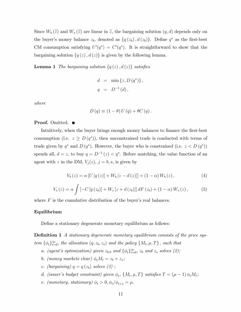
Since Wb (z) and Ws (z) are linear in z, the bargaining solution (q, d) depends only on

the buyer’s money balance zb, denoted as {q (zb) , d (zb)}. Define q∗ as the first-bestCM consumption satisfying U ′(q∗) = C ′(q∗). It is straightforward to show that the

bargaining solution {q (z) , d (z)} is given by the following lemma.

Lemma 1 The bargaining solution {q (z) , d (z)} satisfies

d = min {z,D (q∗)} ,

q = D−1 (d) ,

where

D (q) ≡ (1− θ)U (q) + θC (q) .

Proof. Omitted.

Intuitively, when the buyer brings enough money balances to finance the first-best

consumption (i.e. z ≥ D (q∗)), then unconstrained trade is conducted with terms of

trade given by q∗ and D (q∗). However, the buyer who is constrained (i.e. z < D (q∗))

spends all, d = z, to buy q = D−1 (z) < q∗. Before matching, the value function of an

agent with z in the DM, Vj(z), j = b, s, is given by

Vb (z) = α [U [q (z)] +Wb [z − d (z)]] + (1− α)Wb (z) , (4)

Vs (z) = α

∫[−C [q (zb)] +Ws [z + d (zb)]] dF (zb) + (1− α)Ws (z) , (5)

where F is the cumulative distribution of the buyer’s real balances.

Equilibrium

Define a stationary degenerate monetary equilibrium as follows:

Definition 1 A stationary degenerate monetary equilibrium consists of the price sys-

tem {φt}∞t=0, the allocation (q, zb, zs) and the policy {Mt, µ, T} , such thata. (agent’s optimization) given zb,0 and {φt}∞t=0, zb and zs solves (2);b. (money markets clear) φtMt = zb + zs;

c. (bargaining) q = q (zb) solves (3) ;

d. (issuer’s budget constraint) given φt, {Mt, µ, T} satisfies T = (µ− 1)φtMt;

e. (monetary, stationary) φt > 0, φt/φt+1 = µ.

11

Since Ws (z) and Vs (z) are linear, if a seller buys money in the period t CM and

resells it in the period t+ 1 CM, the rate of return in terms of utility is βφt+1/φt− 1 =

β/µ − 1. Therefore, whenever µ < β, the seller’s money demand zs is infinite, and

hence the money market cannot be cleared. On the other hand, when µ > β, we must

have zs = 0. Intuitively, sellers have no need to spend money in the DM, and thus they

have no incentive to buy money in the CM as long as its rate of return is negative (i.e.

µ > β). Similarly, a buyer will choose to bring an infinite amount for the next CM

when µ < β. When µ > β, a buyer will not bring a money balance that is not intended

to be used in a DM match. In other words, the cash-in-advance constraint, d ≤ zb, is

always binding in the DM when µ > β. In this case, using Lemma 1 and ignoring the

constant terms, we can rewrite the buyer’s optimization problem (2) in the CM as

maxq{− [µ− β (1− α)]D (q) + βαU (q)} , s.t. q ≤ q∗. (6)

Intuitively, a buyer chooses q in the DM and acquires the real balance for the DM

trade D (q). With probability α, there is a trade and the benefit from consumption is

βU (q). With probability 1−α, the money holding is not spent and has a continuationvalue of βD (q). Therefore, [µ− β (1− α)]D (q) captures the net cost of acquiring the

money. A buyer will choose q = zb = 0 when βαU ′ (0) − [µ− β (1− α)]D′ (0) < 0,

simplified to

zb = 0⇔ µ ≥ µ ≡ β

(1 +

αθ

1− θ

).

Therefore, the monetary equilibrium does not exist when µ ≥ µ. For a buyer, since the

opportunity cost of carrying nominal balances is increasing in the money growth rate

µ, and the return from carrying balances for trade is also increasing in the bargaining

weight θ, there is no incentive to hold money when µ is too high, α is too low or θ is

too low. These are the three ineffi ciencies highlighted in the monetary literature: the

cash-in-advance constraint, the search friction and the holdup problem. The following

proposition characterizes the equilibrium.

Proposition 1 A monetary equilibrium exists iff µ ∈ [β, µ). If µ > β, then q < q∗; if

µ→ β, then q = q∗.

According to this proposition, the first-best allocation with q = q∗ cannot be sup-

ported when µ > β. The idea is that, to consume q∗ in the next DM, a buyer

12

needs to acquire µD (q∗) money balances in the CM. So the marginal utility gain

with respect to q is βαU ′(q∗), while the marginal cost of acquiring the balance is

[µ− β (1− α)]D′ (q∗) = [µ− β (1− α)]U ′(q∗). As a result, a buyer has an incentive to

marginally reduce q below q∗ when

(β − µ)U ′(q∗) < 0, (7)

which is true whenever β < µ.

So deflating the economy at the discount rate is necessary and suffi cient for im-

plementing the first-best allocation. Furthermore, the money issuer’s budget con-

straint implies that a positive lump-sum tax is needed (i.e., a negative transfer Tt =

(β − 1)φtMt < 0) to implement the first best. If the money issuer has no taxation

power, then this simple lump-sum transfer scheme cannot implement the first best.

The natural question is: can the first best be supported by using more general trans-

fer schemes (than a lump-sum scheme)? The question calls for a mechanism design

approach to examine general transfer functions.

Summary

In this section, we learned that in a monetary economy with lump-sum transfers,

1. a monetary equilibrium does not exist when money growth is too high, trades

are too infrequent or the buyer’s bargaining power is too low;

2. without taxation, the first-best allocation can never be achieved.

3 Optimal Money Mechanism

The previous section showed that the first-best allocation is not implementable by a ba-

sic, lump-sum transfer scheme. However, the previous setting understates the power of

mechanism design. A natural question is whether the first-best allocation is achievable

when the money issuer can implement any (including sophisticated) non-lump-sum

transfer scheme. In this regard, we use a mechanism design approach to design the

optimal mechanism and interpret the money issuer as the mechanism designer who can

conduct an intervention at night after the CM is closed. We consider the following

13

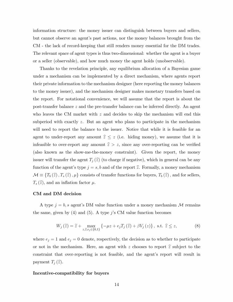
information structure: the money issuer can distinguish between buyers and sellers,

but cannot observe an agent’s past actions, nor the money balances brought from the

CM - the lack of record-keeping that still renders money essential for the DM trades.

The relevant space of agent types is thus two-dimensional: whether the agent is a buyer

or a seller (observable), and how much money the agent holds (unobservable).

Thanks to the revelation principle, any equilibrium allocation of a Bayesian game

under a mechanism can be implemented by a direct mechanism, where agents report

their private information to the mechanism designer (here reporting the money balances

to the money issuer), and the mechanism designer makes monetary transfers based on

the report. For notational convenience, we will assume that the report is about the

post-transfer balance z and the pre-transfer balance can be inferred directly. An agent

who leaves the CM market with z and decides to skip the mechanism will end this

subperiod with exactly z. But an agent who plans to participate in the mechanism

will need to report the balance to the issuer. Notice that while it is feasible for an

agent to under-report any amount z ≤ z (i.e. hiding money), we assume that it is

infeasible to over-report any amount z > z, since any over-reporting can be verified

(also known as the show-me-the-money constraint). Given the report, the money

issuer will transfer the agent Tj (z) (to charge if negative), which in general can be any

function of the agent’s type j = s, b and of the report z. Formally, a money mechanism

M≡ {Tb (z) , Ts (z) , µ} consists of transfer functions for buyers, Tb (z) , and for sellers,

Ts (z), and an inflation factor µ.

CM and DM decision

A type j = b, s agent’s DM value function under a money mechanismM remains

the same, given by (4) and (5). A type j’s CM value function becomes

Wj (z) = z + maxz,z,ej∈{0,1}

{−µz + ejTj (z) + βVj (z)} , s.t. z ≤ z, (8)

where ej = 1 and ej = 0 denote, respectively, the decision as to whether to participate

or not in the mechanism. Here, an agent with z chooses to report z subject to the

constraint that over-reporting is not feasible, and the agent’s report will result in

payment Tj (z).

Incentive-compatibility for buyers

14

It is straightforward to establish that the bargaining solution under a money mech-

anismM is still characterized by Lemma 1. Using the linearity of Wb (z) and ignoring

the constant terms, we can reformulate the buyer’s problem under mechanismM as

maxq,z,eb∈{0,1}

{ebTb (z)− [µ− β (1− α)]D (q) + βαU (q)} , s.t. (9)

z ≤ D (q) . (10)

Here, a buyer who decides not to participate in the mechanism just brings z = D (q)

to the next DM, which will allow the buyer to consume q. A buyer who decides to

participate and intends to have a post-transfer balance of z = D (q) needs to bring

µD (q) − Tb (z) from the CM, and report z ≤ D (q), which will allow the buyer to

consume q in the following DM.

Definition 2 An allocation (q, zb, zs) is incentive compatible for buyers under a money

mechanismM if eb = 1,z = zb, and q = q (zb) solves (9).

To induce buyers to participate in the mechanism (i.e. e = 1), it is necessary to

have an incentive-compatible allocation (q, zb, zs) satisfying

Tb (zb)− [µ− β (1− α)]D (q) + βαU (q) ≥ maxq′{− [µ− β (1− α)]D (q′) + βαU (q′)} .

(11)

Here, the left-hand side (LHS) captures the payoff for participating in the mechanism,

and the right-hand side (RHS) captures the payoff for skipping it.

Incentive-compatibility for sellers

Similarly, using the linearity of Ws (z), and ignoring the constant terms, one can

reformulate the seller’s problem in the CM as

maxz,z,es∈{0,1}

{−µz + esTs (z) + βz} , s.t. z ≤ z. (12)

Here, a seller not participating in the mechanism has no reason to bring money and

thus the additional payoff is zero. A seller who decides to participate and intends to

have a post-transfer balance of z needs to bring µz − Ts (z) from the CM, and report

z ≤ z, and this balance will have a continuation value βz.

15

Definition 3 An allocation (q, zb, zs) is incentive compatible for sellers under a money

mechanismM if es = 1 and z = z = zs solve (12).

Notice that, conditional on es = 0, the value of (12) is zero. So to induce sellers to

participate in the mechanism, it is necessary to have an incentive-compatible allocation

(q, zb, zs) that satisfies

(β − µ) zs + Ts (zs) ≥ 0. (13)

Here, the LHS captures the payoff for participating in the mechanism, and the RHS

captures the payoff for skipping it.

Money issuer’s budget constraint

A money issuer has to balance its budget, or self-finance:

Definition 4 A money mechanismM ≡ {Tb (z) , Ts (z) , µ} is self-financed under theallocation (q, zb, zs) if

Tb (zb) + Ts (zs) = (µ− 1) (zb + zs) . (14)

This budget constraint states that the issuer’s total expenditure on transfers (LHS)

has to be financed by money creation (RHS). The total real balances are zb + zs at

the beginning of a period, and µ (zb + zs) at the end of a period. The RHS denotes

the total balances created within a period. Notice that if an allocation (q, zb, zs) is

incentive compatible for buyers and sellers under a mechanismM, then the equilibrium

conditions in the definition are satisfied.

Implementation of the first best

We are interested in whether the first-best allocation can be implemented. The

following definition introduces this concept formally.

Definition 5 A money mechanismM implements the first best if

a. there exists (zb, zs) such that the first-best allocation (q∗, zb, zs) is incentive com-

patible for buyers and sellers; and

b. M is self-financed under the first-best allocation (q∗, zb, zs).

16

Define a threshold level θ of the buyer’s bargaining power given by

θ ≡ 1− β[1− β (1− α)]

[1− C(q∗)

U(q∗)

] ,which is decreasing in β and α. Note that θ ∈ (0, 1) iff

βα

1− β (1− α)U (q∗) > C (q∗) . (15)

We are going to assume that this condition holds throughout the paper. Intuitively,

when a buyer brings cash from the CM to finance the first-best trade q∗ with the first

seller matched in the subsequent DMs, the maximum (discounted) utility gain from this

future DM trade is βαU (q∗) [1+β(1−α)+β2(1−α)2+ ...] = βαU (q∗) /[1−β (1− α)].

The minimum price the buyer needs to pay to induce the seller to trade is C (q∗). When

the above condition is violated, the maximum gain is lower than the minimum price,

and hence there is no hope for first-best trade in a monetary economy in which agents

need to bring cash to trade.

The following proposition characterizes the implementability of the first-best allo-

cation under an optimally designed money mechanism.

Proposition 2 There exists a money mechanismM that implements the first best if

and only if θ ≥ θ.

Proof. See the appendix.

In the previous section, Proposition 1 shows that, without any authority to enforce

taxation, the first-best allocation cannot be achieved by simple lump-sum transfers.

This is because buyers have an incentive to marginally reduce q below q∗ when (7) is

satisfied (i.e. β < µ). According to Proposition 2, a well-designed mechanism can still

implement the first best. To do that, the transfer scheme Tb (z) has to be designed

to induce buyers to carry the right amount of money balances to finance the first-best

trade. In particular, when the transfer scheme is non-linear and optimally designed, a

buyer no longer has the marginal incentive to reduce q below q∗ even when β < µ. To

give a concrete example, a mechanism may make a big transfer to buyers who bring and

report a suffi ciently high money balance, and make no transfers to buyers who bring

and report too little balances. In an equilibrium in which all buyers co-operate and

17

receive big transfers, inflation is high. Hence, a deviator who brings too little money

and receives no transfers will suffer a loss in purchasing power. Under this non-linear

scheme, buyers do not want to lower their money holding too much because that will

significantly reduce their surplus from DM trades. This explains why the first best can

be supported by the optimal mechanism. However, the power of this scheme is limited

by the size of a buyer’s DM trade surplus, which in turn depends on θ. That explains

why the first best can no longer be supported when θ is too low.

Characterization of optimal mechanism

The above discussion suggests that, to support the first best, transfers to buyers

are needed, and hence money growth is positive. The following proposition formally

establishes this finding, which characterizes all optimal money mechanisms.

Proposition 3 If a money mechanism M ≡ {Tb (z) , Ts (z) , µ} implements the firstbest, then µ > 1.

Proof. Suppose there exists a mechanism M ≡ {Tb (z) , Ts (z) , µ} that implementsthe first best with µ ≤ 1. Then from the proof of Proposition 2, we have

− [1− β (1− α)]D (q∗) + βαU (q∗) ≥ Tb (zb)− [µ− β (1− α)] d∗ + βαU (q∗) ,

≥ maxq′{− [µ− β (1− α)]D (q′) + βαU (q′)} ,

≥ maxq′{− [1− β (1− α)]D (q′) + βαU (q′)} ,

which is a contradiction, since q∗ is the maximizer to the last line only if β = 1.

Simple examples

To illustrate the basic idea, suppose that α = 1. We propose a simple example of

a direct mechanism, and then an example of an indirect mechanism.

(i) Direct mechanism

This simple mechanism makes no transfers to sellers, so Ts (z) = 0 for all z. The

money growth is set to µ = µ and the money created is used to finance transfers to

buyers such that

Tb (z) =

{(µ− 1)D (q∗) , if z = D (q∗)

0, otherwise..

18

First, note that µ > 1 when θ ≥ θ, so that a buyer with z = D (q∗) can receive

a positive transfer (µ− 1)D (q∗) > 0 from the money issuer. As a result, this buyer

has a payoff which equals to −D (q∗) + βU (q∗), which is positive iff θ ≥ θ. Under

this mechanism, a buyer with z 6= D (q∗) does not receive transfers, and thus has a

non-positive payoff because µ = µ. Notice that this scheme is non-linear with respect

to the buyer’s money holding z.

(ii) Indirect mechanism: fixed fee and interest payments

Following Andolfatto (2010), we derive in Appendix A an indirect mechanism with

the following features: the money issuer imposes a fixed fee B on buyers, who can then

collect interest on their money balances at the rate R at the end of the CM:

R =µ

β− 1,

B = (1− β)D (q∗) .

We show that, for suffi ciently high µ, the first-best allocation can be supported if

θ ≥ θ. The basic idea is that the interest payment offsets the buyers’opportunity

cost of carrying money balances to the DM. This interest payment is financed by the

fixed fee paid by the buyers. In order to induce them to pay this fee, the monetary

growth has to be suffi ciently high so that non-participants’trade surplus in the DM is

suffi ciently low. Notice that this scheme is piecewise linear: a fixed fee plus a linear

transfer with respect to the buyer’s money holding z.

Summary

In this section, we learned that:

1. the first best cannot be achieved by any money mechanism when the buyer’s bar-

gaining power is too low, the buyer is too impatient or trades are too infrequent;

2. a non-linear transfer scheme and monetary expansion are essential features of a

money mechanism to implement the first best;

3. the first best can be implemented by a simple indirect mechanism with interest

on buyers’balances, financed by fixed fees and monetary expansion.

19

4 Electronic Money with Limited Participation

The type of money modelled so far is rather primitive —merely a durable, inert object

for circulation. To capture recent innovations, we introduce different payment technolo-

gies. Suppose there is an e-money issuer who maintains the supply of another medium

of exchange, e-money, in addition to money. E-money shares all the basic properties

of money: it is divisible, durable, portable and cannot be counterfeited. However, as

noted in the introduction and will be discussed in greater detail in this section, e-money

is fundamentally different from money. As with the money issuer in the previous sec-

tion, the e-money issuer can distinguish between buyers and sellers. But the e-money

issuer does not have any record-keeping technology, and therefore cannot observe an

agent’s portfolio of money z or e-money n. Otherwise, again, the first best may be

trivially implemented. The lack of record-keeping can be interpreted as some off-line

payment systems where the issuer cannot trace agents’balances in real time. Agents

thus report their portfolio of money and e-money to the e-money issuer, and the e-

money issuer makes transfers based on the report. In this section, we are interested in

an economy where the money mechanism takes as given an exogenous money growth

rate µ ≥ 1 (with lump-sum money transfers given by T = (µ− 1) (zb + zs) ≥ 0).

This assumption simplifies the political economy, since there is no strategic interaction

between the money issuer and the e-money issuer.14 Moreover, we assume that the

e-money issuer has to follow the same growth rate µ of money. This is to capture the

fact that real-world e-money products often involve this feature (e.g. denominated in

cash or convertible at par), and the fact that the e-money issuer, private or public,

often takes inflation as given, and sets the supply to be accommodative to the e-money

demand. Note that removing this restriction will only make the e-money issuer more

powerful, and strengthen our conclusion.

E-money mechanism

Next we introduce the first payment technology: an e-money issuer is able to restrict

participation in an e-money payment system. Specifically, the e-money issuer has the

14In a companion paper, we study the equilibrium interaction between money and e-money in arelated environment.

20

power to exclude agents from holding e-money in the DM, before or after trades. Notice

that the e-money issuer still does not know or control how e-money is used by agents.

Furthermore, the usage of money is unrestricted.

Again, suppose the e-money issuer conducts an intervention at the end of the CM.

We use mechanism design to characterize the optimal mechanism. Let ej = 1 indicate

that a type j = b, s agent chooses to participate in the e-money mechanism. Any

agent choosing ej = 0 will be excluded from the e-money system and cannot hold

any e-money balances in the next DM. Since agents are anonymous, this penalty can

last only one period. An e-money mechanism ME consists of two e-money transfer

functions based on the portfolio reported, denoted asME ≡ {Tb (z, n) , Ts (z, n)}.

CM and DM decision

In the DM, the buyer’s value function under an e-money mechanismME, Vb (z, n, eb),

is

Vb (z, n, eb) = αebes {U [q (z + n)] +Wb [z + n− d (z + n)]} (16)

+α (1− eseb) {U [q (z)] +Wb [z + n− d (z)]}

+ (1− α)Wb (z + n) .

Here, since z and n are already denominated in the unit of the numeraire, the continu-

ation value in the CM, Wb (a), depends only on the sum of the real balances of money

z and e-money n, that is, a ≡ z + n. The first term captures the case when there is

a trading opportunity, and both the buyer and the seller participate in the e-money

system (i.e. eb = es = 1). In this case, the buyer can use the total real balances

a to finance the trade. The second term captures the case when there is a trading

opportunity, but at least one of them does not participate in the e-money system (i.e.

ebes = 0). In this case, the buyer can only use the money z to finance the trade. The

third term captures the case when there is no trading opportunity. The CM value

function of the buyer under an e-money mechanismME is given by

Wb (a) = a+ maxz,n,z,n,eb∈{0,1}

{−µ (z + n) + ebTb (z, n) + βVb (z, n, eb)} , s.t. (17)

z ≤ z, n ≤ n.

21

Again, the constraint restricts that the buyer cannot over-report z, n. In the DM, the

value function, Vs (a, es), of a seller under the e-money mechanismME, is

Vs (a, es) = αeseb{−C [q (zb + nb)] +Ws [a+ d (zb + nb)]} (18)

+α (1− eseb) {−C [q (zb)] +Ws [a+ d (zb)]}

+ (1− α)Ws (a) .

Similarly, if ebes = 1, then the buyer can use zb + nb to finance the trade. If ebes = 0,

then the buyer can only use zb to finance the trade. In the CM, the seller’s value

function under an e-money mechanismME, Ws (a), is

Ws (a) = a+ maxz,n,z,n,es∈{0,1}

{−µ (z + n) + esTs (z, n) + (1− es) βVs (z + n, es)} , s.t.

(19)

z ≤ z, n ≤ n.


It is straightforward to establish that the bargaining solution under an e-money

mechanismME is still characterized by Lemma 1. Using the linearity of Wb (a), and

ignoring the constant terms, one can reformulate the buyer’s problem in the CM under

es = 1 as

maxeb∈{0,1},z,z,n,q

{− [µ− β (1− α)]D (q) + ebTb (z, n) + βαU (q)} , s.t. (20)

z ≤ z, n ≤ D (q)− z.

As before, if eb = 0, the buyer brings µD (q) money balances to buy q in the DM. If

the buyer chooses eb = 1 and intends to have a post-transfer portfolio of (z, n), the

buyer needs to obtain total balances µD (q) − Tb (z, n) from the CM, report z and n,

and then buy q in the following DM.

Definition 6 An allocation (q, zb, zs, nb, ns) is incentive compatible for buyers under

an e-money mechanism ME if eb = 1, z = z = zb, n = nb and q = q (zb + nb) solves

(20) given es = 1.

22

To induce buyers to participate in the mechanism, it is necessary to have an

incentive-compatible allocation (q, zb, zs, nb, ns) satisfying

Tb (zb, nb)−[µ− β (1− α)]D (q)+βαU (q) ≥ maxq′{− [µ− β (1− α)]D (q′) + βαU (q′)} .

(21)

Here, the LHS captures the payoff for joining the e-money mechanism, and the RHS



Similarly, using the linearity of Ws (a), and ignoring the constant terms, one can

reformulate the seller’s problem in the CM under eb = 1 as

maxes∈{0,1},z,z,n,n

{−µ (z + n) + (1− es) β [z + n+ α [d (zb)− C [q (zb)]]]

+esTs (z, n) + esβ [z + n+ α [d (zb + nb)− C [q (zb + nb)]]]

}, s.t.

(22)

z ≤ z, n ≤ n.

Again, a seller joining the e-money mechanism (i.e. es = 1) has to bring extra balances

to pay for the transfer Ts (z, n).

Definition 7 An allocation (q, zb, zs, nb, ns) is incentive compatible for sellers under

an e-money mechanismME if es = 1, z = z = zs, n = n = ns solve (22) under eb = 1.

To induce sellers to participate in the mechanism, it is necessary to have an incentive-

compatible allocation (q, zb, zs, nb, ns) satisfying

Ts (zs, ns)− (µ− β) (zs + ns) + βα [D (q)− C (q)] ≥ βα {d (zb)− C [q (zb)]} , (23)

where the LHS captures the payoff for participating in the e-money mechanism, and

the RHS captures the payoff for skipping it.

E-money issuer’s budget constraint

An e-money issuer has to balance its budget, or self-finance:

23

Definition 8 An e-money mechanismME = {Tb (z, n) , Ts (z, n)} is self-financed withlimited participation under the allocation (q, zb, zs, nb, ns) if

Tb (zb, nb) + Ts (zs, ns) = (µ− 1) (nb + ns) . (24)

Here, the e-money issuer finances transfers to buyers and sellers by issuing e-money

balances.

Implementability of first best

Definition 9 An e-money mechanismME implements the first best with limited par-

ticipation if

a. there exists (zb, zs, nb, ns) such that the first-best allocation (q∗, zb, zs, nb, ns) is

incentive compatible for buyers and sellers; and

b. ME is self-financed with limited participation under the first-best allocation

(q∗, zb, zs, nb, ns).

Define Θ (θ) as the solution to

− (1− β)U (q∗)+[βα + (1− β) θ] [U (q∗)− C (q∗)] = maxq{βαU (q)− [Θ− β (1− α)]D (q)} ,

and set Θ (θ) = ∞ if a solution Θ ≥ β does not exist. The following proposition

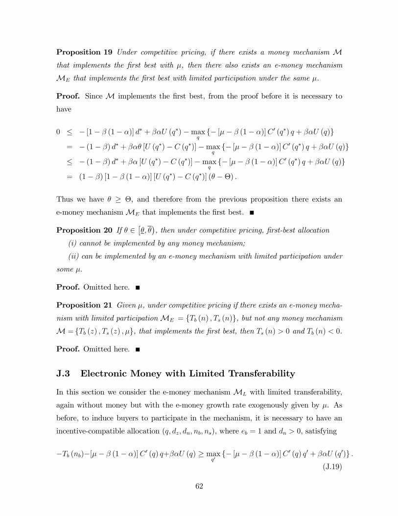
establishes the condition under which the first best can be achieved by an optimal

e-money mechanism with limited participation.

Proposition 4 There exists an e-money mechanismME that implements the first best

with limited participation if and only if µ ≥ Θ (θ).


This proposition shows that, to implement the first best using this e-money mech-

anism, buyers’bargaining power and inflation need to satisfy µ ≥ Θ (θ). An increase

in µ facilitates the implementation of first best because it reduces the outside option

of non-participants who use money only as their means of payment.15 However, an

increase in θ has two opposite effects. On the one hand, it helps achieve the first best

15Interestingly, this is consistent with a popular view that inflation induces agents to adopt somee-money products. For example, Bitcoin is considered by some to be a safe haven from inflation.

24

because the holdup problem is less severe and thus buyers have higher incentives to

bring the right e-money balances. On the other hand, it increases the outside option of

non-participants who also face a less severe holdup problem when using money. But,

in general, we know that Θ (0) = ∞. Therefore, by continuity of Θ, the first best is

not implementable for θ too low, which will be discussed in the following section.

Essentiality of limited participation

Proposition 5 If there exists a money mechanism M that implements the first best

with µ, then there also exists an e-money mechanism ME that implements the first

best with limited participation under the same µ.

Proof. Since M implements the first best, from the proof of Proposition 2 it is

necessary to have

0 ≤ − [1− β (1− α)]D (q∗) + βαU (q∗)−maxq{− [µ− β (1− α)]D (q) + βαU (q)}

= − (1− β)D (q∗) + βαθ [U (q∗)− C (q∗)]−maxq{− [µ− β (1− α)]D (q) + βαU (q)}

≤ − (1− β)U (q∗) + [βα + (1− β) θ] [U (q∗)− C (q∗)]

−maxq{− [µ− β (1− α)]D (q) + βαU (q)} .

Thus we have µ ≥ Θ (θ). Then, from Proposition 4 there exists an e-money mechanism

ME that implements the first best.

This proposition implies that, fixing the money growth rate, an optimal e-money

mechanism featuring limited participation is at least as good as an optimal money

mechanism in implementing the first-best allocation. This result may not hold in gen-

eral when the e-money mechanism has to operate under a money growth rate different

from that associated with the optimal money mechanism. Define

θ ≡ [1− β (1− α)] θ − βα1− β .

The following proposition gives conditions under which the e-money mechanism can

outperform a money mechanism.

Proposition 6 (Essentiality of e-money with limited participation) If θ ∈[θ, θ),

then the first-best allocation

25

(i) cannot be implemented by any money mechanism;

(ii) can be implemented by an e-money mechanism with limited participation under

some µ.

Proof. Omitted here.

This proposition establishes the essentiality of e-money featuring limited partic-

ipation. Part (i), implied by Proposition 2, states that no money mechanism can

implement the first best when θ < θ. At the risk of being repetitive, we reproduce

here the intuition: a money mechanism uses a non-linear transfer scheme to induce

buyers to “co-operate”and to carry suffi cient money balances. This scheme relies on

the “punishment”of eroding deviating buyers’DM trade surplus by not giving them a

transfer. However, the power of this scheme is limited by the size of the buyers’trade

surplus, which depends on θ. When θ < θ, the buyers’trade surplus is insuffi cient for

inducing them to carry the right money balances. In the extreme case of θ → 0, buyers

have no surplus to be extracted.

The ability of the e-money issuer to limit participation provides an additional tool.

By threatening to exclude agents from participating in the e-money system, the issuer

can extract extra resources (especially from sellers), and use those extra resources to

induce buyers to bring the right money balances. How much resources can be extracted

from buyers and sellers? The answer is equal to the difference between the trade surplus

of an e-money user and that of a money user. The power of this scheme is maximized

when money users’ trade surplus is zero, and this will happen when µ ≥ µ (from

Proposition 1). In this case, the threat to exclude deviators allows the issuer to extract

the whole of the (discounted) trade surplus, which equals to βα[U(q∗) − C(q∗)]. This

explains why e-money featuring limited participation is essential.

The power of this scheme is still insuffi cient to achieve first best when θ is too

low (i.e. θ ≤ θ). To illustrate by an extreme example, suppose that µ = 1 and

θ → 0. In this case, the buyer has no bargaining power and thus the price for q∗ is

D (q∗) = U(q∗). So to induce buyers to bring D (q∗) in the previous CM, the transfer

Tb has to be suffi ciently negative that they still have a positive payoff:

Tb − [µ− β (1− α)]D (q∗) + βαU(q∗)−maxq{− [µ− β (1− α)]D (q) + βαU (q)} ≥ 0.

However, the above discussion implies that the maximum transfer the e-money issuer

26

can make is Tb = βα[U(q∗) − C(q∗)], which is the whole of the (discounted) trade

surplus. Plugging µ = 1, D (q) = U(q) and Tb = βα[U(q∗)− C(q∗)] into the LHS, the

buyers’payoff becomes

− [1− β (1− α)]U(q∗) + βα[U(q∗)− C(q∗)] + βαU(q∗)

= −(1− β)[U(q∗)− C(q∗)] + {βαU(q∗)− [1− β (1− α)]C(q∗)} ≥ 0.

As βαU(q∗) − [1 − β (1− α)]C(q∗) → 0, the LHS becomes negative, which is a con-

tradiction. Therefore, this example shows that, when θ is small and βαU(q∗) − [1 −β (1− α)]C(q∗) is small (but remains positive, as assumed), the first-best allocation

is not implementable by any e-money mechanism with limited participation. This

explains part (ii) of the above proposition.

Overall, Propositions 2 and 6 characterize the implementability of first best using

the money mechanism and e-money mechanism. When buyers’bargaining power is

high (θ ≥ θ), an optimal money mechanism can implement the first best. Hence, e-

money is not essential relative to money in this region. When buyers’bargaining power

is moderate (θ > θ ≥ θ), only e-money featuring limited participation can implement

the first best, given suffi ciently high money growth µ. Hence, e-money is essential

relative to money in this region. Finally, when buyers’bargaining power is too low

(θ > θ), even an e-money featuring limited participation may not implement the first

best.16

Characterization of optimal e-money mechanism

After establishing the essentiality of e-money, we next characterize the optimal

e-money mechanism.

Proposition 7 Given µ, if there exists an e-money mechanism with limited participa-

tionME = {Tb (z, n) , Ts (z, n)}, but not any money mechanismM = {Tb (z) , Ts (z) , µ},that implements the first best, then Ts (z, n) < 0 and Tb (z, n) > 0.

Proof. See the appendix.16Notice that e-money may remain essential in this region. Even though it cannot implement the

first best, it may still improve the allocation.

27

As mentioned above, when θ is too low, extracting trade surplus from buyers alone

cannot raise enough resources to support the first best. The power of limited participa-

tion helps implement the first best by extracting surplus from sellers (i.e. Ts (z, n) < 0)

to cross-subsidize buyers’holding of e-money balances (i.e. Tb (z, n) > 0). The key ben-

efit of limiting participation is allowing cross-subsidization from sellers to buyers, which

is infeasible under a money mechanism.

Simple examples

Suppose that α = 1, µ > µ and θ ∈ [θ, θ). So according to Proposition 6, e-money

with limited participation is essential. We will illustrate examples of simple direct and

indirect mechanisms. In these extreme examples, sellers get zero trade surplus, but

more general cases can be similarly constructed.


Under this simple mechanism, the transfer function for sellers is a fixed fee:

Ts(zs, ns) = −β[D (q∗)− C(q∗)] for any (zs, ns),

and the transfer function for buyers is

Tb(zs, nb) =

{(β + µ− 1)D (q∗)− βC(q∗), if nb = D (q∗)

0, otherwise..

When µ > µ, Proposition 1 implies that buyers not joining the e-money mechanism

will choose not to trade. In this case, a buyer joining the e-money mechanism needs to

bring βC(q∗) + (1− β)d∗ from the CM, receive a transfer Tb from the issuer, and bring

D (q∗) into the DM to consume q∗. We can show that the participation constraint is

satisfied when

θ ≥ θ =θ − β1− β .

Notice that this scheme exhibits the features of non-linear transfers and cross-

subsidization.

(ii) Indirect mechanism: fixed membership fee and proportional rewards

The e-money issuer imposes a fixed membership fee Bb on buyers, who can then

28

collect interest on their money balances at the rate R in the end of the CM:

R =µ

β− 1,

Tb = (2β − 1)D (q∗)− βC(q∗).

Without paying Bb, a buyer cannot use e-money in the next DM. Similarly, in order

to receive e-money in the next DM, a seller has to pay

Ts = −β[D(q∗)− C(q∗)].

The e-money issuer’s budget is balanced. Obviously, sellers are indifferent between

joining or not. Buyers have an incentive to join when

Tb −D(q∗)β + βU(q∗) ≥ 0,

where βD(q∗) is the balance they need to bring to the DM so that, after the interest

payment, they have real balance D(q∗) to finance the effi cient quantity in the DM. One

can show that this is positive when θ ≥ θ. Notice that this scheme also exhibits the

features of piecewise linear transfers and cross-subsidization. This mechanism does not

involve money. Appendix B considers an example involving money deposits. In that

example, the e-money mechanism is designed to support the positive value of money

in equilibrium.

Summary


1. When buyers have moderate bargaining power and the money growth rate is

high, an e-money mechanism with limited participation is essential to implement

the first best.

2. Given the money growth rate, an optimal e-money mechanism with limited par-

ticipation is always more essential than any money mechanism; i.e. there are

scenarios where the former, rather than the latter, can achieve the first best.

In this case, cross-subsidization from sellers to buyers is an essential feature to

implement the first best.

29

3. The first best can be implemented by a simple indirect mechanism with fixed

membership fees on buyers and sellers, and proportional rewards on buyers’bal-

ances.

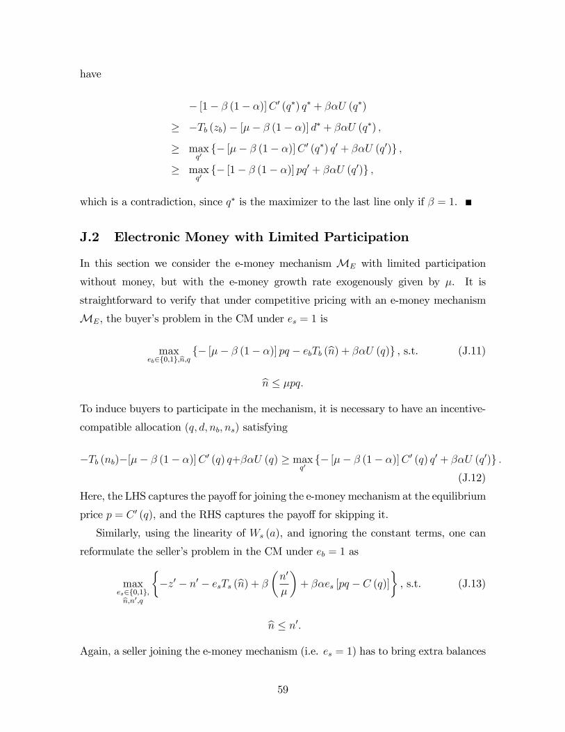
5 Electronic Money with Limited Transferability

Next we consider limited transferability as an alternative feature of e-money. Suppose

that the e-money issuer can no longer limit the participation of users, but has instead

the power to block e-money transfers among agents in the DM. However, the e-money

issuer again does not have any record-keeping technology, and therefore does not know

the amount of e-money transferred or the true identities of the payer and payee. In the

DM, a payer chooses whether to pay the e-money issuer ∆b units of e-money in order to

transfer e-money to someone else. If this fee is not paid, then the e-money transfer will

be blocked by the issuer. Similarly, a payee chooses whether to pay the e-money issuer

∆s units of e-money in order to receive e-money from someone else. Otherwise, the

transfer is blocked. We interpret ∆b and ∆s as interchange fees. We focus on the case

∆b + ∆s ≥ 0, in which otherwise buyers and sellers can fake DM trades (by sending

and receiving an arbitrary small amount of e-money) to earn the transfer ∆b + ∆s

from the e-money issuer. Notice that limited transferability is different from limited

participation: in a mechanism with limited participation, agents need to pay fees to

join the e-money mechanism, in order to use e-money in the DM; in a mechanism with

limited transferability, agents first match in the DM and then decide whether to pay

the interchange fees for using e-money as the means of payment, regardless of whether

they have joined the e-money mechanism in advance. An important distinction is

that a mechanism featuring limited participation collects fees only in the CM, while

a mechanism featuring limited transferability can also collect fees in the DM. This

distinction leads to different abilities to implement the first-best allocation.17 In the

CM, e-money is assumed to be freely transferable among agents.18

CM and DM decision17Note that the money issuer does not need to be physically present in a bilateral match in order

to collect the interchange fees. Instead, in the absence of a zero-sum constraint, part of the balancestransferred can be destroyed automatically in the payment process.18Allowing the issuer to have the additional power to restrict transferability in the CM can only

strengthen our findings.

30

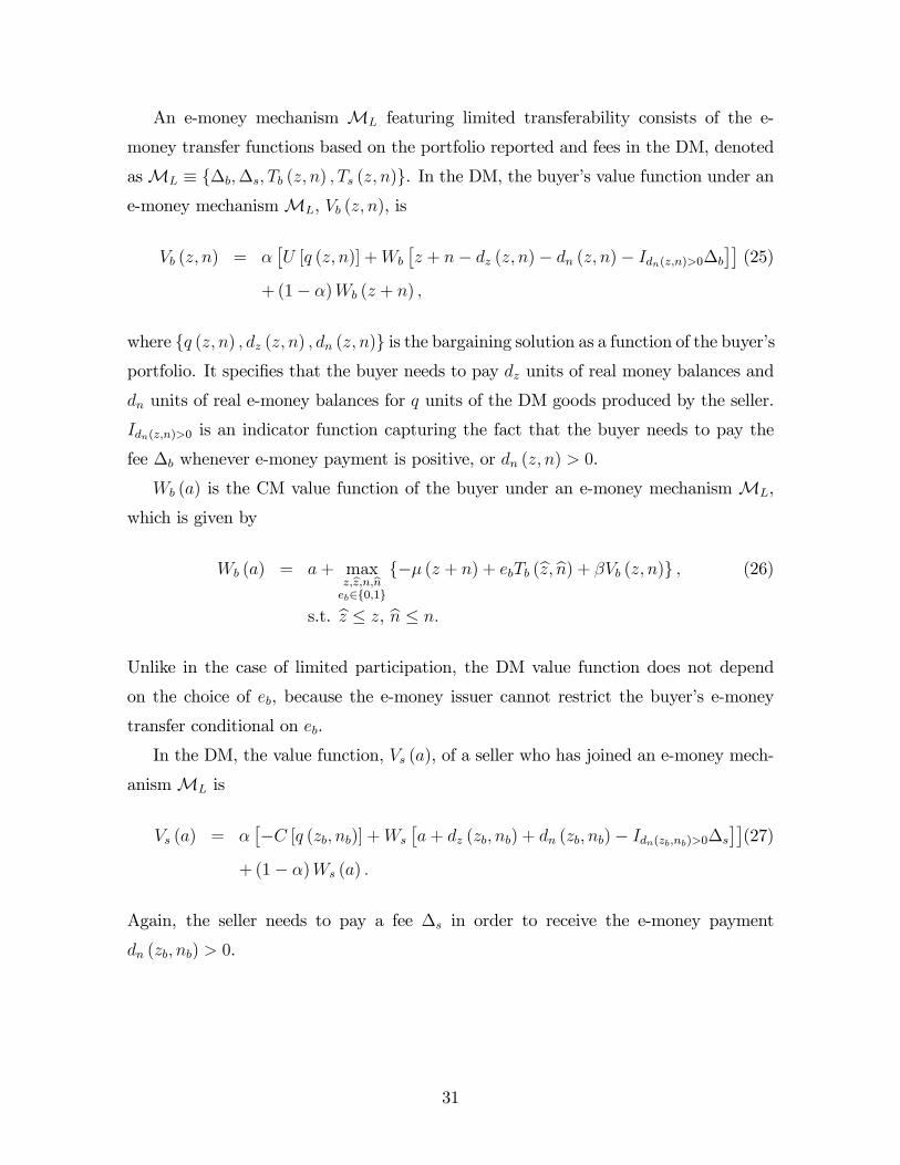
An e-money mechanism ML featuring limited transferability consists of the e-

money transfer functions based on the portfolio reported and fees in the DM, denoted

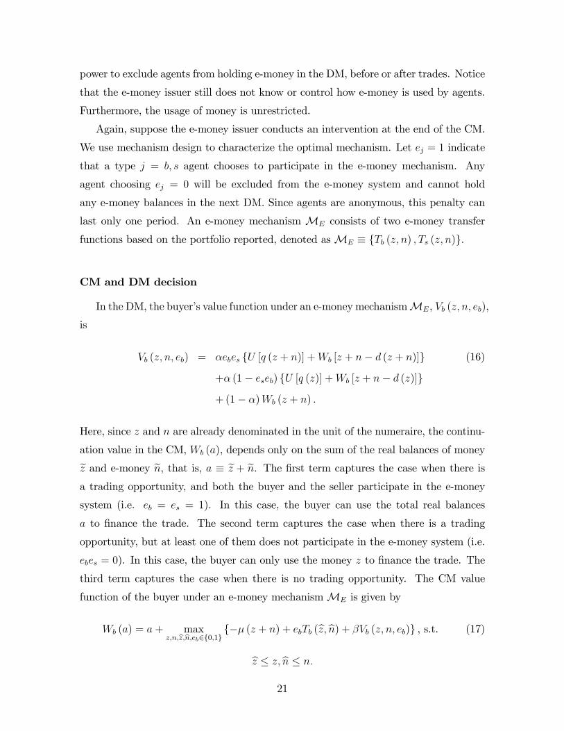
asML ≡ {∆b,∆s, Tb (z, n) , Ts (z, n)}. In the DM, the buyer’s value function under ane-money mechanismML, Vb (z, n), is

Vb (z, n) = α[U [q (z, n)] +Wb

[z + n− dz (z, n)− dn (z, n)− Idn(z,n)>0∆b

]](25)

+ (1− α)Wb (z + n) ,

where {q (z, n) , dz (z, n) , dn (z, n)} is the bargaining solution as a function of the buyer’sportfolio. It specifies that the buyer needs to pay dz units of real money balances and

dn units of real e-money balances for q units of the DM goods produced by the seller.

Idn(z,n)>0 is an indicator function capturing the fact that the buyer needs to pay the

fee ∆b whenever e-money payment is positive, or dn (z, n) > 0.

Wb (a) is the CM value function of the buyer under an e-money mechanism ML,

which is given by

Wb (a) = a+ maxz,z,n,neb∈{0,1}

{−µ (z + n) + ebTb (z, n) + βVb (z, n)} , (26)

s.t. z ≤ z, n ≤ n.

Unlike in the case of limited participation, the DM value function does not depend

on the choice of eb, because the e-money issuer cannot restrict the buyer’s e-money

transfer conditional on eb.

In the DM, the value function, Vs (a), of a seller who has joined an e-money mech-

anismML is

Vs (a) = α[−C [q (zb, nb)] +Ws

[a+ dz (zb, nb) + dn (zb, nb)− Idn(zb,nb)>0∆s

]](27)

+ (1− α)Ws (a) .

Again, the seller needs to pay a fee ∆s in order to receive the e-money payment

dn (zb, nb) > 0.

31

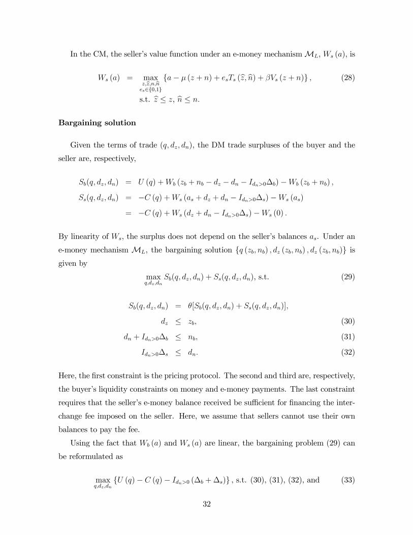
In the CM, the seller’s value function under an e-money mechanismML, Ws (a), is

Ws (a) = maxz,z,n,nes∈{0,1}

{a− µ (z + n) + esTs (z, n) + βVs (z + n)} , (28)

s.t. z ≤ z, n ≤ n.

Bargaining solution

Given the terms of trade (q, dz, dn), the DM trade surpluses of the buyer and the

seller are, respectively,

Sb(q, dz, dn) = U (q) +Wb (zb + nb − dz − dn − Idn>0∆b)−Wb (zb + nb) ,

Ss(q, dz, dn) = −C (q) +Ws (as + dz + dn − Idn>0∆s)−Ws (as)

= −C (q) +Ws (dz + dn − Idn>0∆s)−Ws (0) .

By linearity of Ws, the surplus does not depend on the seller’s balances as. Under an

e-money mechanism ML, the bargaining solution {q (zb, nb) , dz (zb, nb) , dz (zb, nb)} isgiven by

maxq,dz ,dn

Sb(q, dz, dn) + Ss(q, dz, dn), s.t. (29)

Sb(q, dz, dn) = θ[Sb(q, dz, dn) + Ss(q, dz, dn)],

dz ≤ zb, (30)

dn + Idn>0∆b ≤ nb, (31)

Idn>0∆s ≤ dn. (32)

Here, the first constraint is the pricing protocol. The second and third are, respectively,

the buyer’s liquidity constraints on money and e-money payments. The last constraint

requires that the seller’s e-money balance received be suffi cient for financing the inter-

change fee imposed on the seller. Here, we assume that sellers cannot use their own

balances to pay the fee.

Using the fact that Wb (a) and Ws (a) are linear, the bargaining problem (29) can

be reformulated as

maxq,dz ,dn

{U (q)− C (q)− Idn>0 (∆b + ∆s)} , s.t. (30), (31), (32), and (33)

32

(1− θ) [U (q)− dz − dn − Idn>0∆b] = θ [−C (q) + dz + dn − Idn>0∆s] .

Define ∆ ≡ ∆b + ∆s. It is straightforward to show the following lemma, which

characterizes the bargaining solution underML.

Lemma 2 The bargaining solution {q (zb, nb) , dz (zb, nb) , dn (zb, nb)} satisfies:

dz = min {zb, (1− θ)U∗ + θC∗} ,

dn + Idn>0∆b =

min {nb, (1− θ)U∗ + θC∗ + θ∆− dz} ,if nb ≥ ∆ and U (q)− C (q)−∆ ≥ U (q (zb))− C (q (zb))

0, otherwise

D (q) = dz + dn + Idn>0 (∆b − θ∆) .

The key difference from the bargaining solution in the previous section is that the

buyer and the seller now have to share the total interchange fee ∆ according to their

bargaining weights. In the presence of interchange fees, there is a pecking order of

payment: using money before e-money to avoid paying the interchange fees. The

interchange fees partially pass through to prices. From Lemma 2 the total payment

made by the buyer is given by dz + dn + Idn>0∆b = D (q) + Idn>0θ∆, and the total

payment received by the seller is given by dz+dn−Idn>0∆s = D (q)−Idn>0 (1− θ) ∆. A

higher buyer’s bargaining power θ will result in a higher pass-through of the interchange

fees ∆ on the total payment made by the buyer.


Using the linearity of Wb (a), and ignoring the constant terms, one can reformulate

the buyer’s problem in the CM as

maxz,z,n,n,es∈{0,1}

{− (µ− β) (z + n) + ebTb (z, n)

+βα [U [q (z, n)]− dz (z, n)− dn (z, n)− Idn>0∆b]

}, (34)

s.t. z ≤ z, n ≤ n.

Definition 10 An allocation (q, zb, zs, nb, ns) is incentive compatible for buyers under

an e-money mechanismML if eb = 1, z = zb, n = nb, and q solves (34).

33

Notice that a buyer who chooses to skip the mechanismML in CM (i.e., eb = 0)

will not bring e-money to the DM, because money and e-money have the same inflation

rate µ, but using e-money involves an extra interchange fee ∆b, as shown in Lemma

2. Thus, eb = 0 implies nb = dn = 0. As before, to induce buyers to participate in the

mechanism, it is necessary to have an incentive-compatible allocation (q, zb, zs, nb, ns),

where eb = 1 and dn > 0, satisfies

Tb (zb, nb)−[µ− β (1− α)] [D (q) + θ∆]+βαU (q) ≥ maxq′{− [µ− β (1− α)]D (q′) + βαU (q′)} .

(35)




maxz,z,n,n,es∈{0,1}

{(β − µ) (z + n) + esTs (z, n)} , (36)

s.t. z ≤ z, n ≤ n.

Definition 11 An allocation (q, zb, zs, nb, ns) is incentive compatible for sellers under

an e-money mechanismME if es = 1, z = z = zs, n = n = ns solve (36).


compatible allocation (q, zb, zs, nb, ns) such that es = 1 and it satisfies

− (µ− β) (zs + ns) + Ts (zs, ns) ≥ 0. (37)

E-money issuer’s budget constraint

Definition 12 An e-money mechanism ML ≡ {∆b,∆s, Tb (z, n) , Ts (z, n)} is self-financed with limited transferability under the allocation (q, zb, zs, nb, ns) if

Tb (zb, nb) + Ts (zs, ns) = α (∆b + ∆s) + (µ− 1) (nb + ns) . (38)

Implementability of first best

34

Definition 13 An e-money mechanism ML implements the first best with limited

transferability if

a. there exists (zb, zs, nb, ns) such that the first-best allocation (q∗, zb, zs, nb, ns) is

incentive compatible to buyers and sellers; and

b. ML is self-financed with limited transferability under the first-best allocation

(q∗, zb, zs, nb, ns).

As before, define Φ (θ) as the solution to

(β + α− 1)U (q∗)− αC (q∗) = maxq{βαU (q)− [Φ− β (1− α)]D (q)} ,

and set Φ (θ) =∞ if a solution Φ ≥ β does not exist. Notice that Φ (θ) is increasing in

θ for all finite Φ (θ). The following proposition establishes when the optimal e-money

mechanism featuring limited transferability is effi cient.

Proposition 8 There exists some µ and an e-money mechanism ML that imple-

ments the first best with limited transferability if and only if either (a) θ ≥ θ or (b)

(β + α− 1)U (q∗) > αC (q∗). If (a) does not hold, then there existsML implementing

the first best if and only if µ ≥ Φ (θ).


This proposition shows that, to implement the first best using this e-money mech-

anism, buyers’bargaining power and inflation need to satisfy µ ≥ Φ (θ). It is straight-

forward to show that Φ (θ) is increasing in θ. The idea is that an increase in θ raises

the value of the buyers’outside option of non-participation. Higher inflation is needed

to induce them to join the mechanism. Therefore, e-money featuring limited transfer-

ability can implement the first best when inflation is not too low. In particular, when

α = 1, condition (b) in Proposition 8 is always satisfied due to (15). In this case, the

first-best allocation can be achieved for any θ, when the inflation rate is suffi ciently

high.

Essentiality of limited transferability

We first derive conditions under which an optimal mechanism with limited trans-

ferability is at least as good as one with limited participation, and vice versa.

35

Proposition 9 (a) Suppose that θ ≤ α. If there exists an e-money mechanism ME

that implements the first best with limited participation, then there also exists an e-

money mechanismML that implements the first best with limited transferability under

the same µ.

(b) Suppose that θ > α. If there exists an e-money mechanismML that implements

the first best with limited transferability, then there also exists an e-money mechanism

ME that implements the first best with limited participation under the same µ.


Proposition 9 gives a sharp condition θ ≤ α that is suffi cient and necessary for

limited transferability to be at least as essential as limited participation. Before in-

terpreting this condition, we want to check whether there are situations where limited

transferability is strictly more essential than limited participation, and vice versa. The

answer is yes, for both. For example, when α = 1, the condition in part (a) of Propo-

sition 9 is satisfied. In this case, fixing the money growth rate, an optimal e-money

mechanism featuring limited transferability is always at least as good as an optimal

money mechanism in implementing the first-best allocation. More generally, combining

Propositions 4, 8 and 9, we have the following result.

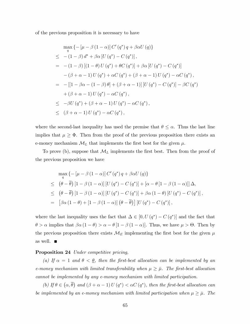
Proposition 10 (Essentiality of e-money with limited transferability) (a) If α =

1 and θ < θ, then the first-best allocation can be implemented by an e-money mechanism

with limited transferability when µ ≥ µ. The first-best allocation cannot be implemented

by any e-money mechanism with limited participation;

(b) If θ ∈(α, θ)and (β + α− 1)U (q∗) < αC (q∗), then the first-best allocation can

be implemented by an e-money mechanism with limited participation when µ ≥ µ. The

first-best allocation cannot be implemented by any e-money mechanism with limited

transferability.


This proposition provides some parameter regions in which there are different or-

ders of essentiality of e-money technologies. In general, limited transferability is more

powerful than limited participation under low θ and high α. The opposite is true under

high θ and low α. What is the intuition? On the one hand, the amount of interchange

fees passed through to the buyer is θ∆, so a low value of θ means that the buyer bears

36

a small interchange fee burden. On the other hand, recall that limited participation

allows the issuer to use exclusion from period t+1 DM as a threat to enforce fees in pe-

riod t. That is why the maximum surplus extractable from a seller, αβ[D (q∗)−C(q∗)],

is discounted, since the fee is paid a period in advance. In contrast, the ability to limit

transferability allows an issuer to extract the seller’s trade surplus in period t DM

by enforcing interchange fees in the same period. The maximum surplus extractable

from a seller becomes α[D (q∗)−C(q∗)], without discounting. Therefore, the gain from

postponing fee collection, which relaxes the seller’s participation constraint, is stronger

when α is high. In sum, for high α the buyer can be rewarded a large sum financed by

the seller’s surplus; for low θ the buyer only bears a small interchange pass-through.

As a result, under high α and low θ the technology limiting transferability can help

induce buyers to bring suffi cient balances to support the first-best allocation, which

cannot be done by the technology limiting participation. But will postponing fee col-

lection tighten the issuer’s budget constraint? No, because the issuer can always create

more e-money balances when needed. From the issuer’s point of view, collecting the

fee in the CM or in the following DM does not matter, as long as the money growth

rate between two CM markets can be maintained at µ. In particular, the issuer can

temporarily create extra e-money balances in CM, and undo them later when inter-

change fees are collected in the following DM. Therefore, limited transferability allows

the e-money issuer to postpone fee collection, maximizing surplus extraction, without

tightening its budget constraint.19

Characterization of optimal e-money mechanism

After establishing the essentiality of e-money, we now characterize the optimal e-

money mechanism.

Proposition 11 Given µ,

(a) if there exists an e-money mechanism with limited transferability

ML = {∆b,∆s, Tb (z, n) , Ts (z, n)}, but not any e-money mechanism with limitedparticipationME , that implements the first best, then ∆ > 0 and Tb (zn, nn) < 0.

19Note that ∂θ/∂β > 0, implying that limited transferability is more essential relative to limitedparticipation when the discount factor is low. A real-world interpretation is that charging interchangefees at the time of the transaction is more desirable relative to charging a membership fee in advance,when the frequency of membership fee payment is low (e.g. annual membership paid a year inadvance).

37

(b) if there exists ME = {Tb (z, n) , Ts (z, n)} but not any ML that implements the

first best, then Ts (z, n) > 0 and Tb (zn, nn) < 0.


As discussed above, to implement the first best, the issuer has to extract trade

surplus in the DM (∆ > 0), which is then used to induce buyers to carry suffi cient

e-money balances in the CM (Tb (zn, nn) < 0). Note that this scheme requires the

issuer to temporarily expand the e-money supply in the CM (to pay buyers Tb (zn, nn))

and later undo it in the DM (by charging fees ∆), ensuring constant money growth

across periods.

Simple examples

Suppose that µ > µ. We will illustrate examples of simple direct and indirect

mechanisms. In these extreme examples, sellers get zero trade surplus, but more general

cases can be similarly constructed.


Under this simple mechanism, the transfer functions are

Tb(zs, nb) =

{µd∗n − C(q∗), if nb = d∗n

0, otherwise.

Ts(zs, ns) = 0, for any (zs, ns),

where d∗n = D(q∗) + θ∆s, and the interchange fees are

∆b = 0,

∆s = d∗ − C(q∗).

The budget constraint of the issuer is satisfied. Obviously, the seller’s participation

constraint is satisfied. When µ > µ, Proposition 1 implies that buyers not joining the e-

money mechanism will choose not to trade. In this case, a buyer has an incentive to join

the e-money mechanism to bring d∗n into the DM to consume q∗ if −C(q∗) + βU(q∗) ≥0, which is always satisfied. This scheme features cross-subsidization from sellers to

buyers, with non-linear pre-trade transfers to buyers, and post-trade fees on sellers.

(ii) Indirect mechanism: fixed membership fee, proportional rewards and inter-

change fee on merchants

38

The e-money issuer imposes a fixed membership fee Bb on buyers, who can then

collect interest on their money balances at the rate R in the end of the CM:

R =µ

β− 1,

Bb = C(q∗)− βd∗n,

where d∗n = D(q∗) + θ∆s. Also, the seller has to pay an interchange fee

∆s = d∗n − C(q∗).

Obviously, sellers are indifferent between joining or not. The issuer’s budget is bal-

anced. Buyers have an incentive to join when

−βd∗n −Bb + βU(q∗) ≥ 0,

where βd∗n is the balance they need to acquire in the CM so that, after interest payment,

they have real balance d∗n to finance the effi cient quantity in the DM. One can show that

this is positive when −C(q∗) + βU(q∗) ≥ 0. This scheme features cross-subsidization

from sellers to buyers, with piecewise linear pre-trade transfers to buyers, and post-

trade fees on sellers. This mechanism does not involve money. Appendix C gives

an example involving money deposits. In that example, the e-money mechanism is

designed to support a positive value of money in equilibrium.

Summary


1. Given a money growth rate, an optimal e-money mechanism with limited trans-

ferability is always more essential than any money mechanism.

2. When buyers have low bargaining power and high frequency of trade, an e-money

mechanism with limited transferability is more essential than any e-money mech-

anism with limited participation (and vice versa). In this case, cross-subsidization

from sellers to buyers using interchange fees is an essential feature to implement

the first best.

39

3. The first best can be implemented by a simple indirect mechanism with fixed

membership fees on buyers, proportional rewards on buyers’balances, and inter-

change fees on sellers.

6 Extension on Competitive Pricing

The above analysis only considers an environment with bilateral trading under the

pricing protocol of proportional bargaining, which is convenient for capturing buyers’

and sellers’bargaining powers and two-sided externalities. One may wonder if our result

is robust in other trading environments. In particular, if agents conduct monetary

trades in a centralized market and take competitive prices as given, they do not consider

other agents’balances and adoption decisions, and do not have any bargaining power.

Even in that environment, however, the curvatures of U and C imply that buyers’and

sellers’surpluses remain positive. As a robustness check, we show in the appendix that

all the main results on essentiality of various money and e-money mechanisms still hold,

if we reinterpret agents’bargaining powers appropriately as the relative trade surplus

at the first best under competitive pricing, θ = [U (q∗)− C ′ (q∗) q∗] / [U (q∗)− C (q∗)].

7 Discussion and Conclusion

Using the mechanism design approach, we have identified several essential features of

e-money that help improve the effi ciency of a monetary economy. First, unlike conven-

tional cash, e-money systems can exclude participation. Second, unlike cash, e-money

systems can restrict and block balance transfers and these transfers are not necessarily

zero-sum bilaterally. Our model then predicts that an optimally designed e-money

system with the above technologies can exhibit several features, including non-linear

pricing, membership fees, interchange fees and rewards to buyers. This prediction does

have some empirical support, since several successful real-world e-money systems also

possess these features. For example, the Octopus card sets a non-linear fee structure,

imposing fixed and variable fees on merchants, and offering rewards and discounts to

40

consumers.20 PayPal also charges merchants a fee on accepting payments.21 Accord-

ing to our model, these pricing features are important components for incentivizing

participants and cross-subsidizing across different types in order to support effi cient

economic outcomes.

The above implications provide useful lessons for policy-makers. First, e-money is

fundamentally different from conventional money. Improved information and technolo-

gies as a result of the introduction of e-money allow more general fee structures and

can increase effi ciency. Second, pricing arrangements such as merchant and interchange

fees can be essential components of an optimal payment system. Hence, fee regula-

tion may distort the optimal mechanism and reduce welfare. For example, the Durbin

Amendment to the Dodd-Frank Act limits the maximum permissible interchange fees

for a debit card transaction based on issuers’costs associated with processing, clearance

and settlement. Our theory suggests that imposing this type of regulation on e-money

can be welfare reducing because the optimal fee is positive even in an environment in

which the physical cost of payments is zero. Third, our theory suggests that different

payment instruments emerge to mitigate different economic frictions. For example,

there is a fundamental difference between money (including e-money) and credit be-

cause consumers need to acquire balances in advance in the former but not the latter

case. The optimal design of a money-based payment system is different from that

of a credit-based system, since they are subject to different incentive and feasibility

constraints. For instance, limiting interchange fees can be optimal for some specific

payment instruments but not all.

While our paper has provided novel economic and policy insights, we have ab-

stracted from several interesting aspects. First, we did not model other potentially

useful features of e-money such as convenience and transaction speed: while these

features can enhance effi ciency, they may not be essential for mitigating fundamental

frictions in a monetary economy. Moreover, additional features of e-money can be eas-

ily incorporated into our environment. Second, we have assumed that there is no cost

20Merchants are subject to a fee structure involving a fixed deposit, a fixed monthly fee and avariable fee proportional to transaction value. Individual buyers need to pay a fixed deposit to obtainan Octopus card. Rewards are offered to cardholders, such as Octopus reward (at least 0.5% ofspending) and discounts on selected products (e.g. transportation).21Under the basic arrangement, PayPal charges a 2.9% merchant fee plus $0.30 per transaction,

with volume discounts applied.

41

of operating an e-money system to highlight the result that the optimal fee on sellers

can be positive even in this extreme setting. In a more general environment, we expect

that a similar pricing arrangement would remain optimal because it could help raise

resources effi ciently to finance the operation of the system. Third, our model focuses

on a simple pricing protocol —proportional bargaining, because it can easily capture

the split of trade surplus between the buyer and the seller. As shown, our finding can

be generalized to other cases, including competitive pricing, where the parameter θ

can be mapped to the share of trade surplus allocated to the buyer under the first-best

allocation. Fourth, we have assumed that trading status (i.e. buyers and sellers) is

permanent because this is more realistic given the frequency of trade captured by the

model. However, our findings will remain unchanged when types are random (espe-

cially when agents know their types before portfolio choice is made). Fifth, we have

not studied the equilibrium outcome when e-money is issued or operated by private

profit-maximizing agents. In a companion paper, Chiu and Wong (2014), we investi-

gate the potential ineffi ciency of the market provision of e-money. Finally, our model

builds on a very standard environment used in the money search literature. Many

alternative model variations (such as endogenous entry and endogenous matching) can

be explored, but we leave those interesting analyses for future work.

42

Appendix

A Proof of Proposition 2

We sketch the proof for Proposition 2 as follows. First, we show that if θ < θ, then

there does not exist any money mechanismM that implements the first best. Suppose

that this is not the case, and denote (q∗, zb, zs) as the first-best allocation implemented.

Since the equilibrium exists as the first-best allocation, we must have µ ≥ β. Denote

η ≡ (β − µ) zs + Ts (zs). Since (q∗, zb, zs) is incentive compatible for sellers, from (13)

we have η ≥ 0. Substituting (14) into the definition of η, we have

Tb (zb)− µzb = −η − (1− β) zs − zb. (A.1)

Since (q∗, zb, zs) is also incentive compatible for buyers, from (11) we have

maxq′{− [µ− β (1− α)]D (q′) + βαU (q′)} ,

≤ Tb (zb)− [µ− β (1− α)] zb + βαU (q∗) ,

= −η − (1− β) zs︸︷︷︸≤0

+(θ − θ

)[1− β (1− α)] [U (q∗)− C (q∗)] ≤ 0,

where we have substituted (A.1) and used the fact that

βαU (q∗)− [1− β (1− α)]D (q∗) ,

= βαU (q∗)− [1− β (1− α)] [(1− θ)U (q∗) + θC (q∗)] ,

=(θ − θ

)[1− β (1− α)] [U (q∗)− C (q∗)] < 0.

Since we have maxq′ {− [µ− β (1− α)]D (q′) + βαU (q′)} ≥ 0, there is a contradiction.

On the other hand, if θ ≥ θ, we can construct a money mechanismM that imple-

ments the first best. Consider the following money mechanism: Ts (z) = 0 for all z,

µ = µ and

Tb (z) =

{(µ− 1)D (q∗) , if z = D (q∗)

0, otherwise.

43

B Implementation by Indirect Mechanisms: Interest-

Bearing Money

So far, we have exploited the power of the revelation principle and focused on the

set of direct mechanisms that implements the first-best allocation when θ ≥ θ. In

general, the reverse of the revelation principle is not true: it is possible to have some

first-best allocations that can be implemented by a direct mechanism, such as the one

constructed above, but not by indirect mechanisms. However, we will show in this

section how an indirect mechanism based on the one proposed by Andolfatto (2010)

can be used to implement the first best when θ ≥ θ.

As with the mechanism suggested by Andolfatto (2010), consider now the money

issuer charges buyers a fixed membership fee B to collect interest on money at the

rate R in the end of the CM. The mechanism has nothing to do with sellers. Thus,

an Andolfatto’s mechanism is indexed by a tripleMA ≡ {B,R, µ}. The optimizationproblem of a buyer in the CM under an Andolfatto’s mechanism can be formulated as

maxz′,q,e∈{0,1}

{e [−z′ −B + βU (q)] + (1− e) [−µD (q) + βU (q)]} , s.t. (B.1)

D (q) =1 +R

µz′. (B.2)

In the equilibrium, we have zb = z′ and zs = 0.

Definition 14 An Andolfatto’s mechanism MA ≡ {B,R, µ} is self-financed underthe allocation (q, d, zb, 0) if

Rzb = B + (µ− 1) zb. (B.3)

Definition 15 An Andolfatto’s mechanismMA implements the first best if

a. z′ = µd∗

1+R= zb, q = q∗ and e = 1 solves (B.1); and

b. MA is self-financed under the first-best allocation (q∗, d∗, zb, 0).

Define µ0 as solution µ = µ0 solving

−d∗ + βU (q∗) = maxq′{−µD (q′) + βU (q′)} . (B.4)

The following lemma shows when µ0 is well-defined.

44

Lemma 3 There exists µ0 solving (B.4) if and only if θ ≥ θ. If such µ0 exists then

µ0 > 1.


The following proposition characterizes the set of an Andolfatto’s mechanism that

implements the first best.

Proposition 12 Suppose that θ ≥ θ. There exists an Andolfatto’s mechanism that

implements the first best, which is constructed as follows:

a. µ ≥ µ0;

b. R = µβ− 1; and

c. B = µ (1− β) d∗.

Proof. Omitted.

C Proof of Proposition 4

First, we want to show that if µ < Θ (θ) then there does not exist an e-money mecha-

nismME that implements the first best with limited participation. Suppose that this

is not the case. Then there exists an e-money mechanism ME that implements the

first best (q∗, zb, zs, nb, ns). Define

η ≡ Ts (zs, ns)− (µ− β) (zs + ns)

+βα [D (q∗)− C (q∗)− d (zb) + C [q (zb)]] .

The fact that (q∗, zb, zs, nb, ns) is incentive compatible for sellers and buyers implies

that η ≥ 0 and D (q∗) = zb + nb. Substituting (24) and D (q∗) = zb + nb to (23), we

have

Tb (zb, nb)− [µ− β (1− α)]D (q∗) = −η − A− βαC (q∗)− (1− β)D (q∗) , (C.1)

where

A ≡ βα [d (zb)− C [q (zb)]] + (µ− β) zs + (µ− 1) zb + (1− β)ns ≥ 0.

45

Notice that the definition of Θ (θ) implies that µ < Θ (θ) if and only if

[βα (1− θ) + [1− β (1− α)]

(θ − θ

)][U (q∗)− C (q∗)] < max

q{− [µ− β (1− α)]D (q) + βαU (q)} .

(C.2)

Since (q∗, zb, zs, nb, ns) is also incentive compatible for buyers, from (21) we have

maxq{− [µ− β (1− α)]D (q) + βαU (q)}

≤ Tb (zb, nb)− [µ− β (1− α)]D (q∗) + βαU (q∗)

= −η − A− (1− β)D (q∗) + βα [U (q∗)− C (q∗)]

= −η − A+[βα (1− θ) +

(θ − θ

)[1− β (1− α)]

][U (q∗)− C (q∗)]

< −η − A+ maxq{− [µ− β (1− α)]D (q) + βαU (q)} ,

where we have substituted (C.1), (C.2) and used the fact that D (q∗) − C (q∗) =

(1− θ) [U (q∗)− C (q∗)]. A contradiction.

On the other hand, if µ ≥ Θ (θ), we can construct an e-money mechanismME that

implements the first best with limited participation. Since µ ≥ Θ (θ), we have ε0 ≡− (1− β)D (q∗)+βα [U (q∗)− C (q∗)]−maxq {− [µ− β (1− α)]D (q) + βαU (q)} ≥ 0.

Fix any nb > 0 and zb > 0 such that nb + zb = D (q∗) and

βα [d (zb)− C [q (zb)]] + (µ− 1) zb ≤ ε0.

Consider the first-best allocation (q∗, zb, 0, nb, 0) and the following e-money mechanism

ME:

Ts (z, n) = βα [D (q∗)− C (q∗)− d (zb) + C [q (zb)]] , (C.3)

Tb (z, n) =

{−Ts (zn, nn) + (µ− 1)nb, if z = zb and n = nb

0, otherwise. (C.4)

Then it is straightforward to verify that (C.3) implies (23) and that (C.4) implies

(24) under the first-best allocation (q∗, zb, 0, nb, 0) and ME constructed above. So

(q∗, zb, 0, nb, 0) is incentive compatible for sellers underME, andME is self-financed

with limited participation. Finally, substituting µd∗ = zb+nb, and (C.4) into− [µ− β (1− α)]D (q∗)−

46

Tb (zb, nb) + βαU (q∗)−maxq {− [µ− β (1− α)]D (q) + βαU (q)}, we have

Tb (zb, nb)− [µ− β (1− α)]D (q∗) + βαU (q∗)−maxq{− [µ− β (1− α)]D (q) + βαU (q)}

= − [µ− β (1− α)]D (q∗) + (µ− 1) (zb + nb) + βα [D (q∗)− C (q∗)] + βαU (q∗)

−βα [d (zb)− C [q (zb)]]− (µ− 1) zb + maxq{− [µ− β (1− α)]D (q) + βαU (q)}

≥ − (1− β)D (q∗) + βα [U (q∗)− C (q∗)]−maxq{− [µ− β (1− α)]D (q) + βαU (q)} − ε0

= ε0 − ε0 = 0.

Therefore, (21) is satisfied given the first-best allocation (q∗, zb, 0, nb, 0) andME con-

structed above. Thus (q∗, zb, 0, nb, 0) is also incentive compatible for buyers underME,

andME implements the first best with limited participation.

D Proof of Proposition 7

Suppose that this is not the case, i.e., there does not exist any money mechanism

but an e-money mechanism ME = {Tb (z, n) , Ts (z, n)} that implements some first-best allocation (q∗, zb, zs, nb, ns) with some µ and Ts (zn, nn) ≤ 0. Consider a first-

best allocation (q∗, z′b, z′s) under a money mechanism M = {Tb (z) , Ts (z) , µ}, where

z′b = zb + nb, z′s = 0, Ts (z) = 0 for all z, and

Tb (z) =

{Tb (zn, nb) + A, if z = z′b0, otherwise,

where

A ≡ (µ− 1) (ns + nb + zs + zb) + Ts (zn, nn) .

Notice that A ≥ 0 due to the premise Ts (zn, nn) ≥ 0. Then it is straightforward to

verify that (13) is satisfied under the first-best allocation (q∗, z′b, z′s) with M, since

z′s = Ts (z) = 0. Also, notice that

Tb (zb)− [µ− β (1− α)] d∗ + βαU (q∗)

= Tb (zn, nb)− [µ− β (1− α)]D (q∗) + βαU (q∗)− A

≥ maxq{− [µ− β (1− α)]D (q) + βαU (q)} − A,

47

where the last inequality comes from the fact that (q∗, zb, zs, nb, ns) is incentive compat-

ible to buyers underME. So (11) is satisfied under the first-best allocation (q∗, z′b, z′s)

withM. Finally, it is straightforward to verify that (14) is satisfied under the first-best

allocation (q∗, z′b, z′s) with M. Thus (q∗, z′b, z

′s) is incentive compatible to buyers and

sellers under M, and M is self-financed. This leads to a contradiction, since there

exists a money mechanismM that implements the first best. Given µ ≥ 1, the result

that Ts (zn, nn) < 0 implies Tb (zn, nn) > 0 from the e-money issuer’s budget (24).

E Implementation by Indirect Mechanisms with lim-

ited participation: Membership-Reward-Deposit

E-money

Proposition 4 states that when θ ≥ Θ (θ, µ), there exists a non-empty set of direct

mechanisms that implements the first-best allocation with limited participation. We

are also interested in constructing some simple indirect mechanisms that can implement

the first-best allocation with limited participation. Consider that the e-money issuer

charges sellers a fixed membership fee Bs to use e-money in the coming DM. To use

e-money, buyers have to maintain a deposit of at least zb units of real money balances,

for a return in terms of a fixed reward −Bb units of real e-money balances, and a

proportional reward at a rate R to load e-money in the CM. The deposit can be used

in the DM. Thus, a membership-reward-deposit mechanism is indexed by MM ≡{Bs, Bb, R, zb}. The optimization problem of a buyer in the CM under a membership-

reward-deposit mechanism can be formulated as

maxz′,n′,q,q′,eb∈{0,1}

{e [−z′ − n′ + βU (q)] + (1− e) [−µD (q′) + βU (q′)]} , s.t. (E.1)

D (q) =z′ −Bb

µ+

1 +R

µn′,

z′ ≥ zb.

48

The optimization problem of a seller in the CM under a membership-reward-deposit

mechanism can be formulated as

maxes∈{0,1}

{e [−Bs + β [d− C (q)]] + (1− e) β

[d

(zbµ

)− C

[q

(zbµ

)]]}. (E.2)

Definition 16 A membership-reward-deposit mechanism MM ≡ {Bs, Bb, R, zb} isself-financed under the allocation (q, d, zb, 0, nb, 0) if

0 = Bs +Bb −R

1 +R(nb +Bb) +

(1− µ−1

)nb. (E.3)

Definition 17 A membership-reward-deposit mechanism MM implements the first

best if

a. z′ = zb, n′ =nb+Bb1+R

, q = q∗ and eb = 1 solves (E.1);

b. es = 1 solves (E.2);

c. MM is self-financed under the first-best allocation (q∗, d∗, zb, 0, nb, 0).

Define ε0 ≡ − (1− β) d∗ + β [U (q∗)− C (q∗)] − maxq {−µD (q) + βU (q)}, whereε0 ≥ 0 if and only if θ ≥ Θ (θ, µ). The following proposition characterizes the set of

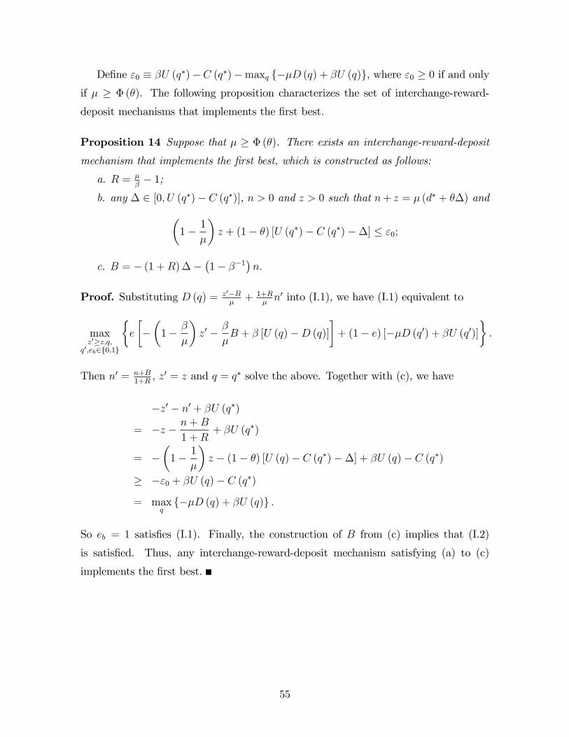
membership-reward-deposit mechanisms that implements the first best.

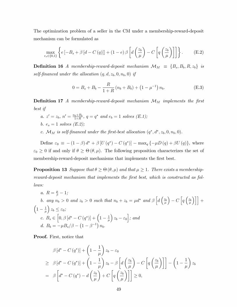
Proposition 13 Suppose that θ ≥ Θ (θ, µ) and that µ ≥ 1. There exists a membership-

reward-deposit mechanism that implements the first best, which is constructed as fol-

lows:

a. R = µβ− 1;

b. any nb > 0 and zb > 0 such that nb + zb = µd∗ and β[d(zbµ

)− C

[q(zbµ

)]]+(

1− 1µ

)zb ≤ ε0;

c. Bs ∈[0, β [d∗ − C (q∗)] +

(1− 1

µ

)zb − ε0

]; and

d. Bb = −µBs/β −(1− β−1

)nb.

Proof. First, notice that

β [d∗ − C (q∗)] +

(1− 1

µ

)zb − ε0

≥ β [d∗ − C (q∗)] +

(1− 1

µ

)zb − β

[d

(zbµ

)− C

[q

(zbµ

)]]−(

1− 1

µ

)zb

= β

[d∗ − C (q∗)− d

(zbµ

)+ C

[q

(zbµ

)]]≥ 0,

49

so the set[0, β [d∗ − C (q∗)] +

(1− 1

µ

)zb − ε0

]in (c) is well-defined. Combining (b)

and (c), we have

−Bs + β [d∗ − C (q∗)] ≥ β

[d

(zbµ

)− C

[q

(zbµ

)]],

so es = 1 satisfies (E.2). Substituting D (q) = z′−Bbµ

+ 1+Rµn′ into (E.1), we have (E.1)

equivalent to

maxz′≥zb,q,

q′,eb∈{0,1}

{e

[−(

1− β

µ

)z′ − β

µBb + β [U (q)−D (q)]

]+ (1− e) [−µD (q′) + βU (q′)]

},

(E.4)

where n′ = nb+Bb1+R

, z′ = zb and q = q∗ solve the above. Substituting (c) and (d) into

−(

1− βµ

)zb − β

µBb + β [U (q∗)−D (q∗)], we have

−(

1− β

µ

)zb −

β

µBb + β [U (q∗)−D (q∗)]

≥ −(

1− βµ

)(zb + nb) + β [U (q∗)− C (q∗)]− ε0

= maxq{−µD (q) + βU (q)} .

So eb = 1 satisfies (E.1). Finally, the construction of Bb from (d) implies that (E.3)

is satisfied. Thus, any membership-reward-deposit mechanism that satisfies (a) to (d)


F Proof of Proposition 8

In the interest of brevity, we show only the later part that if θ < θ, thenML implements

the first best if and only if µ ≥ Φ (θ). The proof of the rest of Proposition 8 just follows

the proof of Proposition 4. Define

η ≡ Ts (zs, ns)− (µ− β) (zs + ns) .

The fact that (q∗, zb, zs, nb, ns) is incentive compatible for sellers and buyers implies that

η ≥ 0 and D (q∗)+θ∆−∆b = zb+nb. Substituting (38) and D (q∗)+θ∆−∆b = zb+nb

50

into (37), we have

Tb (zb, nb)− [µ− β (1− α)] [D (q∗) + θ∆] + βαU (q∗) (F.1)

= −A− (1− β)U (q∗) + [1− β (1− α)] θ [U (q∗)− C (q∗)]

+ [α− θ [1− β (1− α)]] ∆,

where

A = η +

(1− 1

µ

)∆b + (µ− 1) zb + (µ− β) zs + (1− β)ns ≥ 0.

To show the "if" part, notice that there exists ML such that A = 0 and ∆ =

U (q∗)−C (q∗). Obviously, the corresponding (q∗, zb, zs, nb, ns) with A = 0 is incentive

compatible for sellers underML. Also, the right-hand side of (F.1) becomes

− (1− β)U (q∗) + [1− β (1− α)] θ [U (q∗)− C (q∗)]

+ [α− θ [1− β (1− α)]] [U (q∗)− C (q∗)] ,

= (β + α− 1)U (q∗)− αC (q∗) ,

≥ maxq{βαU (q)− [µ− β (1− α)]D (q)} ,

where the last line uses the premise that µ ≥ Φ (θ). Thus (q∗, zb, zs, nb, ns) is incentive

compatible for buyers underML, and hence implements the first best. Notice that the

above part is true whether or not the premise θ < θ is true, since the proof does not

depend on the condition θ < θ.

To show the "only if" part, suppose that there exists ML implementing the first

best for some µ. Then, (F.1) becomes

maxq{βαU (q)− [µ− β (1− α)]D (q)}

≤ − (1− β)U (q∗) + [1− β (1− α)] θ [U (q∗)− C (q∗)]

+ [α− θ [1− β (1− α)]] ∆,

=(θ − θ

)[1− β (1− α)] [U (q∗)− C (q∗)] + [α− θ [1− β (1− α)]] ∆.

Under the premise θ < θ, the first term on the last line is negative; thus, the second

term must be positive in order to not be less than the non-negative first line. Thus,

we must have α− θ [1− β (1− α)] > 0. Since ∆ ≤ [U (q∗)− C (q∗)], then the last line

51

is less than (β + α− 1)U (q∗)− αC (q∗). Thus we have reached µ ≥ Φ (θ).

G Proof of Proposition 9

To prove (a), suppose that ME implements the first best. Then from the proof of

Proposition 4 it is necessary to have

maxq{− [µ− β (1− α)]D (q) + βαU (q)}

≤ − (1− β)D (q∗) + βα [U (q∗)− C (q∗)] ,

= − (1− β) [(1− θ)U (q∗) + θC (q∗)] + βα [U (q∗)− C (q∗)]

− (β + α− 1)U (q∗) + αC (q∗) + (β + α− 1)U (q∗)− αC (q∗) ,

= − [[1− βα− (1− β) θ] + (β + α− 1)] [U (q∗)− C (q∗)]− βC (q∗)

+ (β + α− 1)U (q∗)− αC (q∗) ,

≤ −βU (q∗) + (β + α− 1)U (q∗)− αC (q∗) ,

≤ (β + α− 1)U (q∗)− αC (q∗) ,

where the second-last inequality has used the premise that θ ≤ α. Thus the last line

implies that µ ≥ Φ (θ). Then from the proof of Proposition 8 there exists an e-money

mechanismML that implements the first best for the given µ.

To prove (b), suppose thatML implements the first best. Then from the proof of

Proposition 8 we have

maxq{− [µ− β (1− α)]D (q) + βαU (q)}

≤(θ − θ

)[1− β (1− α)] [U (q∗)− C (q∗)] + [α− θ [1− β (1− α)]] ∆,

≤(θ − θ

)[1− β (1− α)] [U (q∗)− C (q∗)] + βα (1− θ) [U (q∗)− C (q∗)] ,

=[βα (1− θ) + [1− β (1− α)]

(θ − θ

)][U (q∗)− C (q∗)] ,

where the last inequality uses the fact that ∆ ∈ [0, U (q∗)− C (q∗)] and the fact that

θ > α implies βα (1− θ) > α − θ [1− β (1− α)]. Thus, we have µ > Θ (θ). Then by

Proposition 4 there existsME implementing the first best for the given µ as well.

52

H Proof of Proposition 11

In the interest of brevity, we show only (a). Suppose that this is not the case, i.e., there

exists an e-money mechanism ML = {∆b,∆s, Tb (z, n) , Ts (z, n)} that implementssome first-best allocation (q∗, zb, zs, nb, ns) with limited transferability under∆ = 0 and

some µ, but there does not exist any e-money mechanismME = {Tb (z, n) , Ts (z, n)}that implements the first-best allocation with limited participation under the same µ.

Given ∆ = 0, consider a money mechanismML = {T ′b (z) , T ′s (z) , µ} where

T ′s (z) =

{Ts (zs, ns) , if z = zs + ns

0, otherwise

T ′b (z) = Tb (z, n) + (µ− 1) (zb + zs) .

Consider a first-best allocation (q∗, z′b, z′s) where z

′b = zb+nb and z′s = zs+ns. Then it is

straightforward to verify that (13) is satisfied under the first-best allocation (q∗, z′b, z′s)

withM, since (13) and (37) are the same. Also, notice that

Tb (zb)− [µ− β (1− α)]D (q∗) + βαU (q∗)

= Tb (zb, nb)− [µ− β (1− α)]D (q∗) + βαU (q∗) +(1− µ−1

)(zb + zs)

≥ maxq{− [µ− β (1− α)]D (q) + βαU (q)} ,

where the last inequality comes from the fact that (q∗, zb, zs, nb, ns) is incentive compat-

ible to buyers underML. So (11) is satisfied under the first-best allocation (q∗, z′b, z′s)

withM. Finally, it is straightforward to verify that (14) is satisfied under the first-best

allocation (q∗, z′b, z′s) with M. Thus (q∗, z′b, z

′s) is incentive compatible to buyers and

sellers under M, and M is self-financed. This contradicts Proposition 5, since there

exists a money mechanismM that implements the first best but there does not exist

any e-money mechanism ME = {Tb (z, n) , Ts (z, n)} that implements the first-bestallocation with limited participation under the same µ. Therefore, we establish ∆ > 0.

Finally, notice that (9) is satisfied only if Tb (zn, nn) > 0. Thus, we prove Proposition

11.

53

I Implementation by Indirect Mechanisms with Lim-

ited Transferability: Interchange-Reward-Deposit

E-money

Proposition 8 states that when µ ≥ Φ (θ), there exists a non-empty set of direct

mechanisms that implements the first-best allocation with limited transferability. We

are also interested in constructing some simple indirect mechanisms that can implement

the first-best allocation with limited transferability. Consider that to use e-money,

buyers have to maintain a deposit of at least z units of real money balances, for

a return in terms of a fixed reward of −B units of real e-money balances, and a

proportional reward at a rate R to load e-money in the CM. The deposit can be used

in the DM. To receive any positive amount of e-money in the DM, the payee is charged

a fixed interchange fee of ∆ units of real e-money balances from the e-money received.

Thus, an interchange-reward-deposit mechanism is indexed by MI ≡ {∆, B,R, z}.The optimization problem of a buyer in the CM under an interchange-reward-deposit

mechanism can be formulated as

maxz′,n′,q,q′,eb∈{0,1}

{e [−z′ − n′ + βU (q)] + (1− e) [−µD (q′) + βU (q′)]} , s.t. (I.1)

D (q) + θ∆ =z′ −Bµ

+1 +R

µn′,

z′ ≥ z.

Definition 18 An interchange-reward-deposit mechanismMI ≡ {∆, B,R, z} is self-financed under the allocation (q, d, z, n) if

0 = ∆ +B − R

1 +R(n+B) +

(1− µ−1

)z. (I.2)

Definition 19 An interchange-reward-deposit mechanism MI implements the first

best if

a. z′ = z, n′ = n+Bb1+R

, q = q∗ and eb = 1 solves (I.1);

b. MI is self-financed under the first-best allocation (q∗, d∗, z, n).

54

Define ε0 ≡ βU (q∗)−C (q∗)−maxq {−µD (q) + βU (q)}, where ε0 ≥ 0 if and only

if µ ≥ Φ (θ). The following proposition characterizes the set of interchange-reward-

deposit mechanisms that implements the first best.

Proposition 14 Suppose that µ ≥ Φ (θ). There exists an interchange-reward-deposit

mechanism that implements the first best, which is constructed as follows:

a. R = µβ− 1;

b. any ∆ ∈ [0, U (q∗)− C (q∗)], n > 0 and z > 0 such that n+ z = µ (d∗ + θ∆) and(1− 1

µ

)z + (1− θ) [U (q∗)− C (q∗)−∆] ≤ ε0;

c. B = − (1 +R) ∆−(1− β−1

)n.

Proof. Substituting D (q) = z′−Bµ

+ 1+Rµn′ into (I.1), we have (I.1) equivalent to

maxz′≥z,q,

q′,eb∈{0,1}

{e

[−(

1− β

µ

)z′ − β

µB + β [U (q)−D (q)]

]+ (1− e) [−µD (q′) + βU (q′)]

}.

Then n′ = n+B1+R

, z′ = z and q = q∗ solve the above. Together with (c), we have

−z′ − n′ + βU (q∗)

= −z − n+B

1 +R+ βU (q∗)

= −(

1− 1

µ

)z − (1− θ) [U (q)− C (q∗)−∆] + βU (q)− C (q∗)

≥ −ε0 + βU (q)− C (q∗)

= maxq{−µD (q) + βU (q)} .

So eb = 1 satisfies (I.1). Finally, the construction of B from (c) implies that (I.2)

is satisfied. Thus, any interchange-reward-deposit mechanism satisfying (a) to (c)


55

J Competitive Pricing

In this section we show that all the results under proportional bargaining extend to

the environment with competitive pricing. In the DM, agents take a competitive price

p as given. The seller’s DM problem is given by

maxq{−C (q) + pq} . (J.1)

Thus the equilibrium price is given by

p = C ′ (q) . (J.2)

We can rewrite the buyer’s optimization problem in the CM as

maxq{− [µ− β (1− α)] pq + βαU (q)} . (J.3)

The following proposition characterizes the equilibrium.

Proposition 15 Under competitive pricing, a monetary equilibrium exists iff µ ≥ β.

If µ > β, then q < q∗; if µ→ β, then q = q∗.

Proof. A monetary equilibrium exists if q ∈ (0,∞). The first-order condition with

respect to q evaluated at the equilibrium price p = C ′ (q) is then

− [µ− β (1− α)]C ′ (q) + βαU ′ (q) = 0.

Since q ≤ q∗ and hence C ′ (q) ≤ U ′ (q), the above has an interior solution of q ∈ (0,∞)

iff µ ≥ β. Notice that q is strictly decreasing in µ. If µ = β, we have C ′ (q) = U ′ (q)

and hence q = q∗.

J.1 Optimal Money Mechanism

It is straightforward to verify that, under competitive pricing, the buyer’s CM problem

under a money mechanismM is given by

maxq,z,eb∈{0,1}

{−ebTb (z)− [µ− β (1− α)] pq + βαU (q)} , s.t. (J.4)

56

z ≤ µpq. (J.5)

To induce buyers to participate in the mechanism (i.e. eb = 1), it is necessary to have

an incentive-compatible allocation (q, d, zb, zs) satisfying

−Tb (zb)−[µ− β (1− α)]C ′ (q) q+βαU (q) ≥ maxq′{− [µ− β (1− α)]C ′ (q) q′ + βαU (q′)} .

(J.6)

Here, the LHS captures the payofffor participating in the mechanism at the equilibrium

price p = C ′ (q) and d = pq, and the RHS captures the payoff for skipping it.

Similarly, using the linearity of Ws (z), and ignoring the constant terms, one can


maxz′,z,es∈{0,1}

{−z′ − esTs (z) +

β

µz′}, s.t. z ≤ z′. (J.7)

Here, a seller not participating in the mechanism has no reason to bring money and

thus the additional payoff is zero. A seller who decides to participate and intends to

have a post-transfer balance of z needs to bring z + Ts (z) from the CM, and report

z ≤ z′, where the balance will have a continuation value βz′/µ.

Notice that the value after choosing es = 0 is zero. So to induce sellers to participate

in the mechanism, it is necessary to have an incentive-compatible allocation (q, d, zb, zs)

satisfying

−zs − Ts (zs) +β

µzs ≥ 0. (J.8)

Here, the LHS captures the payoff for participating in the mechanism, and the RHS


With abuse of notation, define the share of buyer surplus at the first best as

θ ≡ U (q∗)− C ′ (q∗) q∗U (q∗)− C (q∗)

. (J.9)

The following proposition characterizes the implementability of the first-best allocation

under an optimally designed money mechanism.

Proposition 16 Under competitive pricing, there exists a money mechanismM that

implements the first best if and only if θ ≥ θ.

Proof. We sketch the proof as follows. First, we show that if θ < θ then there does

57

not exist any money mechanismM that implements the first best. Suppose that this

is not the case. Denote (q∗, d∗, zb, zs) as the first-best allocation implemented with

p = C ′ (q∗). Since the equilibrium exists as the first-best allocation, we must have

µ ≥ β. Denote η ≡ −(

1− βµ

)zs − Ts (zs). Since (q∗, d∗, zb, zs) is incentive compatible

for sellers, we have η ≥ 0. The fact that (q∗, d∗, zb, zs) is incentive compatible for buyers

implies that µd∗ = zb. Substituting µd∗ = zb into the definition of η, we have

−Tb (zb)− µd∗ = −η − 1− βµ

zs − d∗. (J.10)

Since (q∗, d∗, zb, zs) is also incentive compatible for buyers, we have

maxq′{− [µ− β (1− α)] pq′ + βαU (q′)} ,

≤ −Tb (zb)− [µ− β (1− α)] d∗ + βαU (q∗) ,

= −η − 1− βµ

zs︸︷︷︸≤0

+(θ − θ

)[1− β (1− α)] [U (q∗)− C (q∗)] ≤ 0,

where we have used the fact that

βαU (q∗)− [1− β (1− α)] d∗,

= βαU (q∗)− [1− β (1− α)] [(1− θ)U (q∗) + θC (q∗)] ,

=(θ − θ

)[1− β (1− α)] [U (q∗)− C (q∗)] < 0.

Since we have maxq′ {− [µ− β (1− α)] pq′ + βαU (q′)} ≥ 0, there is a contradiction.

On the other hand, if θ ≥ θ, we can construct a money mechanismM that imple-

ments the first best. Consider the following money mechanism: Ts (z) = 0 for all z,

µ = µ and

Tb (z) =

{(1− µ) d∗, if z = µd∗

0, otherwise.

Proposition 17 Under competitive pricing, if a money mechanismM ≡ {Tb (z) , Ts (z) , µ}implements the first best, then µ > 1.

Proof. Suppose that there exists a mechanism M ≡ {Tb (z) , Ts (z) , µ} that imple-ments the first best with µ ≤ 1. Then from the proof of the previous proposition, we

58

have

− [1− β (1− α)]C ′ (q∗) q∗ + βαU (q∗)

≥ −Tb (zb)− [µ− β (1− α)] d∗ + βαU (q∗) ,

≥ maxq′{− [µ− β (1− α)]C ′ (q∗) q′ + βαU (q′)} ,

≥ maxq′{− [1− β (1− α)] pq′ + βαU (q′)} ,

which is a contradiction, since q∗ is the maximizer to the last line only if β = 1.

J.2 Electronic Money with Limited Participation

In this section we consider the e-money mechanism ME with limited participation

without money, but with the e-money growth rate exogenously given by µ. It is

straightforward to verify that under competitive pricing with an e-money mechanism

ME, the buyer’s problem in the CM under es = 1 is

maxeb∈{0,1},n,q

{− [µ− β (1− α)] pq − ebTb (n) + βαU (q)} , s.t. (J.11)

n ≤ µpq.

To induce buyers to participate in the mechanism, it is necessary to have an incentive-

compatible allocation (q, d, nb, ns) satisfying

−Tb (nb)−[µ− β (1− α)]C ′ (q) q+βαU (q) ≥ maxq′{− [µ− β (1− α)]C ′ (q) q′ + βαU (q′)} .

(J.12)

Here, the LHS captures the payofffor joining the e-money mechanism at the equilibrium

price p = C ′ (q), and the RHS captures the payoff for skipping it.


reformulate the seller’s problem in the CM under eb = 1 as

maxes∈{0,1},n,n′,q

{−z′ − n′ − esTs (n) + β

(n′

µ

)+ βαes [pq − C (q)]

}, s.t. (J.13)

n ≤ n′.

Again, a seller joining the e-money mechanism (i.e. es = 1) has to bring extra balances

59

to pay for the transfer Ts (n).


compatible allocation (q, d, nb, ns) satisfying

−Ts (ns)−(

1− β

µ

)ns + βα [C ′ (q) q − C (q)] ≥ 0, (J.14)

where the LHS captures the payoff for participating in the e-money mechanism, and

the RHS captures the payoff for skipping it.

Define Θ as the solution to

− (1− β)U (q∗)+[βα + (1− β) θ] [U (q∗)− C (q∗)] = maxq{βαU (q)− [Θ− β (1− α)]C ′ (q∗) q} ,

and set Θ = ∞ if a solution Θ ≥ β does not exist. The following proposition estab-

lishes the condition under which the first best can be achieved by an optimal e-money

mechanism with limited participation.

Proposition 18 Under competitive pricing, there exists an e-money mechanismME

that implements the first best with limited participation if and only if µ ≥ Θ.

Proof. First, we want to show that if µ < Θ, then there does not exist an e-money

mechanismME that implements the first best with limited participation. Suppose that

this is not the case, then there exists an e-money mechanismME that implements a

first best (q∗, d∗, nb, ns). Define

η ≡ −(

1− β

µ

)ns − Ts (ns) + βα [d∗ − C (q∗)] .

The fact that (q∗, d∗, nb, ns) is incentive compatible for sellers and buyers implies that

η ≥ 0 and µd∗ = nb. Then we have

− [µ− β (1− α)] d∗ − Tb (nb) = −η −(

1− βµ

)ns − βαC (q∗)− (1− β) d∗. (J.15)

Notice that the definition of Θ implies that µ < Θ if and only if

[βα (1− θ) + [1− β (1− α)]

(θ − θ

)][U (q∗)− C (q∗)] < max

q{− [µ− β (1− α)]C ′ (q∗) q + βαU (q)} .

(J.16)

60

Since (q∗, d∗, nb, ns) is also incentive compatible for buyers, we have

maxq{− [µ− β (1− α)]C ′ (q∗) q + βαU (q)}

≤ −Tb (nb)− [µ− β (1− α)] d∗ + βαU (q∗)

= −η −(

1− βµ

)ns − (1− β) d∗ + βα [U (q∗)− C (q∗)]

= −η −(

1− βµ

)ns +

[βα (1− θ) +

(θ − θ

)[1− β (1− α)]

][U (q∗)− C (q∗)]

< −η −(

1− βµ

)ns + max

q{− [µ− β (1− α)]D (q) + βαU (q)} .

A contradiction.

On the other hand, if µ ≥ Θ, we can construct an e-money mechanismME that

implements the first best with limited participation. Since θ ≥ Θ, we have ε0 ≡− (1− β) d∗ + βα [U (q∗)− C (q∗)]−maxq {− [µ− β (1− α)]C ′ (q∗) q + βαU (q)} ≥ 0.

Consider the first-best allocation (q∗, d∗, nb, 0) and the following e-money mechanism

ME:

Ts (n) = βα [d∗ − C (q∗)] , (J.17)

Tb (n) =

{−Ts (ns)−

(1− 1

µ

)nb, if z = zb and n = nb

0, otherwise. (J.18)

Then it is straightforward to verify that (q∗, d∗, nb, 0) is incentive compatible for sellers

underME, and thatME is self-financed with limited participation. Finally, substitut-

ing µd∗ = nb into− [µ− β (1− α)] d∗−Tb (nb)+βαU (q∗)−maxq {− [µ− β (1− α)]C ′ (q∗) q + βαU (q)},we have

− [µ− β (1− α)] d∗ − Tb (nb) + βαU (q∗)−maxq{− [µ− β (1− α)]C ′ (q∗) q + βαU (q)}

= − [µ− β (1− α)] d∗ +

(1− 1

µ

)nb + βα [d∗ − C (q∗)] + βαU (q∗)

+ maxq{− [µ− β (1− α)]C ′ (q∗) q + βαU (q)}

≥ − (1− β) d∗ + βα [U (q∗)− C (q∗)]−maxq{− [µ− β (1− α)]C ′ (q∗) q + βαU (q)} − ε0

= ε0 − ε0 = 0.

Thus (q∗, d∗, nb, 0) is also incentive compatible for buyers underME, andME imple-

ments the first best with limited participation.

61

Proposition 19 Under competitive pricing, if there exists a money mechanism Mthat implements the first best with µ, then there also exists an e-money mechanism


Proof. Since M implements the first best, from the proof before it is necessary to

have

0 ≤ − [1− β (1− α)] d∗ + βαU (q∗)−maxq{− [µ− β (1− α)]C ′ (q∗) q + βαU (q)}

= − (1− β) d∗ + βαθ [U (q∗)− C (q∗)]−maxq{− [µ− β (1− α)]C ′ (q∗) q + βαU (q)}

≤ − (1− β) d∗ + βα [U (q∗)− C (q∗)]−maxq{− [µ− β (1− α)]C ′ (q∗) q + βαU (q)}

= (1− β) [1− β (1− α)] [U (q∗)− C (q∗)] (θ −Θ) .

Thus we have θ ≥ Θ, and therefore from the previous proposition there exists an

e-money mechanismME that implements the first best.

Proposition 20 If θ ∈[θ, θ), then under competitive pricing, first-best allocation

(i) cannot be implemented by any money mechanism;

(ii) can be implemented by an e-money mechanism with limited participation under

some µ.


Proposition 21 Given µ, under competitive pricing if there exists an e-money mecha-

nism with limited participationME = {Tb (n) , Ts (n)}, but not any money mechanismM = {Tb (z) , Ts (z) , µ}, that implements the first best, then Ts (n) > 0 and Tb (n) < 0.


J.3 Electronic Money with Limited Transferability

In this section we consider the e-money mechanism ML with limited transferability,

again without money but with the e-money growth rate exogenously given by µ. As

before, to induce buyers to participate in the mechanism, it is necessary to have an

incentive-compatible allocation (q, dz, dn, nb, ns), where eb = 1 and dn > 0, satisfying

−Tb (nb)−[µ− β (1− α)]C ′ (q) q+βαU (q) ≥ maxq′{− [µ− β (1− α)]C ′ (q) q′ + βαU (q′)} .

(J.19)

62

Similarly, to induce sellers to participate in the mechanism, it is necessary to have

an incentive-compatible allocation (q, dz, dn, nb, ns) such that, es = 1, satisfying

−(

1− β

µ

)ns − Ts (ns) ≥ 0. (J.20)

As before, define Φ as the solution to

(β + α− 1)U (q∗)− αC (q∗) = maxq{βαU (q)− [Φ− β (1− α)]C ′ (q∗) q} ,

and set Φ =∞ if a solution Φ ≥ β does not exist. The following proposition establishes

when the optimal e-money mechanism featuring limited transferability is effi cient.

Proposition 22 Under competitive pricing, there exists some µ and an e-money mech-

anismML that implements the first best with limited transferability if and only if either

(a) θ ≥ θ or (b) (β + α− 1)U (q∗) > αC (q∗). If (a) does not hold, then there exists

ML implementing the first best if and only if µ ≥ Φ.

Proof. In the interest of brevity, we show only the latter part that if θ < θ, thenML

implements the first best if and only if µ ≥ Φ. Define

η ≡ −(

1− β

µ

)ns − Ts (ns) .

The fact that (q∗, d∗, nb, ns) is incentive compatible for sellers and buyers implies that

η ≥ 0 and µ (d∗ + ∆b) = nb. The issuer’s budget is

0 = α (∆b + ∆s) + Tb (nb) + Ts (ns) +

(1− 1

µ

)(nb + ns) . (J.21)

Substituting µ (d∗ + ∆b) = nb and the issuer’s budget, we have

− [µ− β (1− α)] (d∗ + ∆b)− Tb (nb) + βαU (q∗)

= − [1− β (1− α)] (d∗ + ∆b) + α∆ + Ts (ns) +

(1− 1

µ

)ns + βαU (q∗)

= −η − (1− β)U (q∗) + [1− β (1− α)] θ [U (q∗)− C (q∗)]

+ [α− θ [1− β (1− α)]] ∆.

To show the "if" part, notice that there existsML such that ∆ = U (q∗)− C (q∗).

Obviously, the corresponding (q∗, dz, dn, nb, ns) with A = 0 is incentive compatible for

63

sellers underML. Then we have

− (1− β)U (q∗) + [1− β (1− α)] θ [U (q∗)− C (q∗)]

+ [α− θ [1− β (1− α)]] [U (q∗)− C (q∗)] ,

= (β + α− 1)U (q∗)− αC (q∗) ,

≥ maxq{βαU (q)− [µ− β (1− α)]C ′ (q∗) q} ,

where the last line uses the premise that µ ≥ Φ (θ). Thus (q∗, dz, dn, zb, zs, nb, ns) is

incentive compatible for buyers underML, and hence implements the first best. Notice

that the above part is true whether or not the premise θ < θ is true, since the proof

does not depend on the condition θ < θ.

To show the "only if" part, suppose there exists ML implementing the first best

for some µ. Then, we have

maxq{βαU (q)− [µ− β (1− α)]C ′ (q∗) q}

≤ − (1− β)U (q∗) + [1− β (1− α)] θ [U (q∗)− C (q∗)]

+ [α− θ [1− β (1− α)]] ∆,

=(θ − θ

)[1− β (1− α)] [U (q∗)− C (q∗)] + [α− θ [1− β (1− α)]] ∆.

Under the premise θ < θ, the first term on the last line is negative, and thus the second

term must be positive in order to be not less than the non-negative first line. Thus, we

must have α − θ [1− β (1− α)] > 0. Since ∆ ≤ [U (q∗)− C (q∗)], the last line is less

than (β + α− 1)U (q∗)− αC (q∗). Thus we have reached µ ≥ Φ.

Proposition 23 Under competitive pricing,

(a) Suppose that θ ≤ α. If there exists an e-money mechanismME that implements

the first best with limited participation, then there also exists an e-money mechanism

ML that implements the first best with limited transferability under the same µ.

(b) Suppose that θ > α. If there exists an e-money mechanismML that implements

the first best with limited transferability, then there also exists an e-money mechanism


Proof. To prove (a), suppose thatME implements the first best. Then from the proof

64

of the previous proposition it is necessary to have

maxq{− [µ− β (1− α)]C ′ (q∗) q + βαU (q)}

≤ − (1− β) d∗ + βα [U (q∗)− C (q∗)] ,

= − (1− β) [(1− θ)U (q∗) + θC (q∗)] + βα [U (q∗)− C (q∗)]

− (β + α− 1)U (q∗) + αC (q∗) + (β + α− 1)U (q∗)− αC (q∗) ,

= − [[1− βα− (1− β) θ] + (β + α− 1)] [U (q∗)− C (q∗)]− βC (q∗)

+ (β + α− 1)U (q∗)− αC (q∗) ,

≤ −βU (q∗) + (β + α− 1)U (q∗)− αC (q∗) ,

≤ (β + α− 1)U (q∗)− αC (q∗) ,

where the second-last inequality has used the premise that θ ≤ α. Thus the last line

implies that µ ≥ Φ. Then from the proof of the previous proposition there exists an

e-money mechanismML that implements the first best for the given µ.

To prove (b), suppose thatML implements the first best. Then from the proof of

the previous proposition we have

maxq{− [µ− β (1− α)]C ′ (q∗) q + βαU (q)}

≤(θ − θ

)[1− β (1− α)] [U (q∗)− C (q∗)] + [α− θ [1− β (1− α)]] ∆,

≤(θ − θ

)[1− β (1− α)] [U (q∗)− C (q∗)] + βα (1− θ) [U (q∗)− C (q∗)] ,

=[βα (1− θ) + [1− β (1− α)]

(θ − θ

)][U (q∗)− C (q∗)] ,

where the last inequality uses the fact that ∆ ∈ [0, U (q∗)− C (q∗)] and the fact that

θ > α implies that βα (1− θ) > α− θ [1− β (1− α)]. Thus, we have µ > Θ. Then by

the previous proposition there existsME implementing the first best for the given µ

as well.

Proposition 24 Under competitive pricing,

(a) If α = 1 and θ < θ, then the first-best allocation can be implemented by an

e-money mechanism with limited transferability when µ ≥ µ. The first-best allocation

cannot be implemented by any e-money mechanism with limited participation.

(b) If θ ∈(α, θ)and (β + α− 1)U (q∗) < αC (q∗), then the first-best allocation can

be implemented by an e-money mechanism with limited participation when µ ≥ µ. The

65

first-best allocation cannot be implemented by any e-money mechanism with limited

transferability.


Proposition 25 Given µ, under competitive pricing,

(a) if there exists an e-money mechanism with limited transferabilityML = {∆b,∆s, Tb (n) , Ts (n)},but not any e-money mechanism with limited participation ME , that implements the

first best, then ∆ > 0 and Tb (nn) < 0.

(b) if there existsME = {Tb (n) , Ts (n)} but not anyML that implements the first

best, then Ts (n) > 0 and Tb (nn) < 0.

Proof. Similar to the proof of Proposition 11.

66

References

[1] Andolfatto, D. 2010. “Essential interest-bearing money.” Journal of Economic

Theory, 145, 4, 1495—1507.

[2] Araujo, L., Camargo, B., Minetti, R., and Puzzello, D. 2012. “The essentiality of

money in environments with centralized trade.”Journal of Monetary Economics,

59(7), 612-621.

[3] Araujo, L. and T. Hu. 2014. “Optimal monetary interventions in credit markets.”

Manuscript.

[4] Cavalcanti, R. and A. Erosa. 2008. “Effi cient propagation of shocks and the opti-

mal return on money.”Journal of Economic Theory, 142(1), 128-148.

[5] Cavalcanti, R. and E. Nosal. 2009. “Some benefits of cyclical monetary policy.”

Economic Theory, 39(2), 195-216.

[6] Chiu, J., and T. Wong. 2014. “E-Money: Effi ciency, Stability and Optimal Policy.”

Bank of Canada Working Paper No. 2014-16.

[7] Committee on Payment and Settlement Systems (CPSS). 2001. “Survey of Elec-

tronic Money Developments.”Bank for International Settlements.

[8] Hu, T., Kennan, J. and N. Wallace. 2009. “Coalition-proof trade and the Friedman

rule in the Lagos-Wright model.”Journal of Political Economy, 117, 116-137.

[9] Hu, T. and G. Rocheteau. 2013. “On the coexistence of money and higher-return

assets and its social role.”Journal of Economic Theory, 148(6), 2520-2560.

[10] Hu, T. and C. Zhang. 2014. “Responding to the inflation tax.”Manuscript.

[11] Kahn, C. M., and Roberds, W. 2009. “Why pay? An introduction to payments

economics.”Journal of Financial Intermediation, 18(1), 1-23.

[12] Kocherlakota, N. 1998. “Money is Memory.” Journal of Economic Theory 81,

232—251.

[13] Kocherlakota, N. 2003. “Societal benefits of illiquid bonds.”Journal of Economic

Theory, 108, 179-193.

67

[14] Kocherlakota, N., and N. Wallace. 1998. “Incomplete record-keeping and optimal

payment arrangements.”Journal of Economic Theory, 81(2), 272-289.

[15] Lagos, R. 2010. “Some results on the optimality and implementation of the Fried-

man rule in the Search Theory of Money.”Journal of Economic Theory, 145(4),

1508-1524.

[16] Lagos, R. and R. Wright. 2005. “A Unified Framework for Monetary Theory and

Policy Analysis.”Journal of Political Economy 113(3), 463-484.

[17] Li, Y. 2011. “Currency and checking deposits as means of payment.”Review of

Economic Dynamics, 14(2), 403-417.

[18] Monnet, C. and W. Roberds. W. 2008. “Optimal pricing of payment services.”

Journal of Monetary Economics, 55(8), 1428-1440.

[19] Rochet, J. C., and Tirole, J. 2003. “Platform competition in two-sided markets.”

Journal of the European Economic Association, 1(4), 990-1029.

[20] Rocheteau, G., 2012. “The Cost of Inflation: A mechanism design approach.”

Journal of Economic Theory, 147 1261-1279.

[21] Rocheteau, G. and R. Wright. 2005. “Money in search equilibrium, in competitive

equilibrium, and in competitive search equilibrium.”Econometrica, 73 (2005) 175—

202.

[22] Rysman, M. 2009. “The economics of two-sided markets.”The Journal of Eco-

nomic Perspectives, 125-143.

[23] Shy, O., and Z. Wang. 2011. “Why do payment card networks charge proportional

fees?”The American Economic Review, 101(4), 1575-1590.

[24] Wallace, N. 2010. “The mechanism-design approach to monetary theory.”Hand-

book of Monetary Economics (Forthcoming).

[25] Wallace, N. 2014. “Optimal money creation in “pure currency”economies: a con-

jecture.”The Quarterly Journal of Economics, 129(1), 259-274.

68

[26] Wang, Z. 2012 “Debit card interchange fee regulation: some assessments and

considerations.”FRB Economic Quarterly, 98(3), 159-183.

69

WORKING PAPERS IN ECONOMICS AND FINANCE

School of Economics and Finance | Victoria Business School | www.victoria.ac.nz/sef

Date post:	27-Mar-2018
Category:	Documents
Upload:	lyhuong
View:	217 times
Download:	1 times

On the essentiality of E-money - Home | Victoria University · PDF file ·...

Documents