SIAM J. APPL. MATH. c! 2006 Society for Industrial and Applied MathematicsVol. 66, No. 4, pp. 1366–1382

ON THE EVOLUTION OF DISPERSAL INPATCHY LANDSCAPES"

STEPHEN KIRKLAND† , CHI-KWONG LI‡ , AND SEBASTIAN J. SCHREIBER‡

Abstract. To better understand the evolution of dispersal in spatially heterogeneous landscapes,we study di!erence equation models of populations that reproduce and disperse in a landscapeconsisting of k patches. The connectivity of the patches and costs of dispersal are determined by ak!k column substochastic matrix S, where Sij represents the fraction of dispersing individuals frompatch j that end up in patch i. Given S, a dispersal strategy is a k!1 vector whose ith entry gives theprobability pi that individuals disperse from patch i. If all of the pi’s are the same, then the dispersalstrategy is called unconditional; otherwise it is called conditional. For two competing populationsof unconditional dispersers, we prove that the slower dispersing population (i.e., the populationwith the smaller dispersal probability) displaces the faster dispersing population. Alternatively, forpopulations of conditional dispersers without any dispersal costs (i.e., S is column stochastic and allpatches can support a population), we prove that there is a one parameter family of strategies thatresists invasion attempts by all other strategies.

Key words. population dynamics, evolution of dispersal, monotone dynamics

AMS subject classifications. 15A48, 39A11, 92D25

DOI. 10.1137/050628933

1. Introduction. Plants and animals often live in landscapes where environ-mental conditions vary from patch to patch. Within patches, these environmentalconditions may include abiotic factors such as light, space, and nutrient availabilityor biotic factors such as prey, competitors, and predators. Since the fecundity andsurvivorship of an individual depends on these factors, an organism may decrease orincrease its fitness by dispersing across the environment. Depending on their phys-iology and their ability to accumulate information about the environment, plantsand animals can exhibit two modes of dispersals and a variety of dispersal strate-gies. Plants and animals can be active dispersers that move by their own energyor passive dispersers that are moved by wind, water, or other animals. Passive dis-persers alter their dispersal rates by varying the likelihood of dispersing and the timespent dispersing [20]. Dispersal strategies can vary from unconditional strategies inwhich the probability of dispersing from a patch is independent of the local envi-ronmental conditions to conditional strategies in which the likelihood of dispersingdepends on local environmental factors. Understanding how natural selection acts onthese di!erent modes and strategies of dispersal has been the focus of much theoreticalwork [2, 5, 8, 10, 12, 15, 16, 17]. For instance, using coupled ordinary di!erential equa-tion models for populations passively dispersing between two patches, Holt [8] showedthat slower dispersing populations could always invade equilibria determined by faster

!Received by the editors April 10, 2005; accepted for publication (in revised form) November 15,2005; published electronically April 21, 2006.

http://www.siam.org/journals/siap/66-4/62893.html†Department of Mathematics and Statistics, University of Regina, Regina, SK S4S 0A2, Canada

(kirkland@math.uregina.ca). The research of this author was supported in part by NSERC.‡Department of Mathematics, The College of William and Mary, Williamsburg, VA 23187-8795

(ckli@math.wm.edu, sjschr@wm.edu). The research of the second author was partially supported byan NSF grant and an HK RCG grant. The second author is an honorary professor of the HeilongjiangUniversity and an honorary professor of the University of Hong Kong. The research of the thirdauthor was partially supported by NSF grants EF-0436318 and DMS-0517987.

1366

EVOLUTION OF DISPERSAL 1367

dispersing populations. Hastings [5] and Dockery et al. [2] considered evolution of dis-persal in continuous space using reaction di!usion equations. Dockery et al. provedthat for two competing populations di!ering only in their di!usion constant, the popu-lation with the larger di!usion constant is excluded. In contrast, McPeek and Holt [17]using a two patch model consisting of coupled di!erence equations found that “dis-persal between patches can be favored in spatially varying but temporally constantenvironment, if organisms can express conditional dispersal strategies.”

In this article, we consider the evolution of conditional and unconditional dis-persers for a general class of multipatch di!erence equations. For these di!erenceequations, individuals in each patch disperse with some probability. When these proba-bilities are independent of location, the population exhibits an unconditional dispersalstrategy; otherwise it exhibits a conditional dispersal strategy. For dispersing individ-uals, the nature of the landscape determines the likelihood Sji that a disperser frompatch i ends up in patch j. Unlike previous studies of the evolution of unconditionaland conditional dispersal [2, 5, 8, 17], we allow for an arbitrary number of patchesand place no symmetry conditions on S. For active dispersers, asymmetries in Smay correspond to geographical and ecological barriers that inhibit movement fromone patch to another. For passive dispersers, these asymmetries may correspond toasymmetries in the abiotic or biotic currents in which they drift.

Our main goal is to determine what types of theorems can be proved about theevolution of dispersal for this general class of di!erence equation models. To achievethese goals, the remainder of the article is structured as follows. In section 2, we intro-duce the models. Under monotonicity assumptions about the growth rates, we provethat either populations playing a single dispersal strategy go extinct for all initial con-ditions or approach a positive fixed point for all positive initial conditions. We alsointroduce models of competing populations that di!er only in their dispersal abilityand prove a result about invasiveness. In section 3, we prove that for two competingpopulations of unconditional dispersers, the slower dispersing population displacesthe faster dispersing population. The proof relies heavily on proving, in section 4,monotonicity of the principal eigenvalue for a one-parameter family of nonnegativematrices. In section 5, we prove that, provided there is no cost to dispersal and allpatches can support a population, there is a one-parameter family of conditionaldispersal strategies that resists invasion from other types of dispersal strategies. Nu-merical simulations suggest that these strategies can displace all other strategies, andwe prove that these strategies can weakly coexist. In section 6, we discuss our findingsand suggest directions for future research.

2. The models and basic results. Consider a population exhibiting discretereproductive and dispersal events and living in an environment consisting of k patches.The vector of population densities is given by x = (x1, . . . , xk)T ! Rk

+, where Rk+ is

the nonnegative cone of Rk. To describe reproduction and survival in each patch, let!i : R+ " R+ denote the per-capita growth rate of the population in the ith patchas a function of the population density in the ith patch. For these per-capita growthrates we make the following assumptions.

A1: !i are positive continuous decreasing functions.A2: limxi#$ !i(xi) < 1.A3: xi #" xi!i(xi) is increasing.

Assumption A1 corresponds to the population exhibiting increasing levels of intraspecific competition or interference as population densities increase. Assumption A2implies that at high densities the population tends to decrease in size. Assumption A3

1368 S. KIRKLAND, C.-K. LI, AND S. J. SCHREIBER

implies that the population does not exhibit overcompensating density dependence:higher densities in the current generation yield higher densities in the next generation.Many models in the population ecology literature satisfy these three assumptions.For instance, see the Beverton–Holt model [1] in which !i(xi) = ai

1+bixiand the Ivlev

model [14] in which !i(xi) = ai(1 $ exp($b xi)).To describe dispersal between patches, we assume that each individual in patch i

disperses with a probability pi and Sji is the probability that a dispersing individualfrom patch i arrives in patch j. About the matrix S we make the following assumption.

A4: S is a k % k primitive column substochastic matrix.S can be column stochastic if all dispersing individuals migrate successfully or sub-stochastic if some dispersing individuals experience mortality. The primitive assump-tion ensures that individuals (possibly after several generations) can move from anypatch to any patch. S characterizes how connected the landscape is for dispersingindividuals. For example, for a fully connected metapopulation, S could be the ma-trix whose entries all equal 1

k ; i.e., an individual is equally likely to end up in anypatch after dispersing. Alternatively, in a landscape with a one-dimensional latticestructure with individuals able only to move to neighboring patches in one time stepS is a column substochastic tridiagonal matrix that is primitive, provided it has apositive entry on the diagonal. From these p and S, the following matrix describeshow the population redistributes itself across the environment in one time step:

Sp = I $ diag (p) + S diag (p),

where diag (p) denotes a diagonal matrix with diagonal entries p1, . . . , pk.If a census of the population is taken before reproduction and after dispersal,

then the dynamics of the population are given by

x% = Sp"(x)x =: F (x),(1)

where x% denotes the population state in the next time step and "(x) is the k % kdiagonal matrix whose ith diagonal entry equals !i(xi).

Our first result characterizes the global dynamics of (1). To state this result, letFn(x) denote F composed with itself n times. Given x, y ! Rk

+, we write x & y ifxi & yi for all 1 ' i ' k, x > y if x & y and x (= y, and x ) y if xi > yi for all1 ' i ' k. For a matrix A, let r(A) denote the spectral radius of A.

Theorem 2.1. Assume that Assumptions A1–A4 hold and p ! (0, 1]k. If r(Sp

"(0)) ' 1, then

limn#$

Fn(x) = 0

for all x & 0. Alternatively, if r(Sp"(0)) > 1, then there exists a fixed point x ) 0for F such that

limn#$

Fn(x) = x

for all x > 0.Proof. Let A(x) = Sp"(x). Assumptions A1, A4, and p ) 0 imply that A(x) is

primitive for all x & 0. Assumption A3 implies that F (x) & F (y) (resp., F (x) > F (y),F (x) ) F (y)) whenever x & y (resp., x > y, x ) y). In other words, F is a stronglymonotone map.

EVOLUTION OF DISPERSAL 1369

Suppose that r(A(0)) ' 1. Let wT ) 0 be a left Perron vector of A(0), i.e.,r(A(0))wT = wTA(0). Define the function L : Rk

+ " R+ by L(x) = wTx. For x > 0,Assumption A1 implies that wTA(0) ) wTA(x). Hence, for any x > 0,

L(F (x)) = wTA(F (x))x

= wTA(0)x + wT (A(F (x)) $A(0))x

< r(A(0))wTx ' L(x).

Since L is strictly decreasing along nonzero orbits of F , L(0) = 0, and L(x) > 0 forx > 0, it follows that limn#$ Fn(x) = 0 for all x & 0.

Suppose r(A(0)) > 1. First, we show that there exists a positive fixed point x.Let v ) 0 be a right Perron eigenvector for A(0), i.e., A(0)v = r(A(0))v. SinceA(0)v ) v, continuity of A(x) implies that there exists " > 0 such that A(y)y ) y,where y = "v. Since F (x) ) F (y) whenever x ) y, induction implies y * F (y) *F 2(y) * F 3(y) * · · · . Assumption A2 implies that the increasing sequence Fn(y) isbounded. Hence, there exists x such that limn#$ Fn(y) = x. Continuity of F impliesthat F (x) = x. Second, we show that limn#$ Fn(x) = x whenever x > x > 0. Inparticular, x is a unique positive fixed point. Let wT be the left Perron eigenvectorof A(x) that satisfies wT x = 1. Since x is a positive fixed point, r(A(x)) = 1. DefineL : Rk

+ " R+ by L(x) = wTx. Let x > x > 0. Then x > F (x) > 0 and

L(F (x)) = wTA(F (x))x

= wTA(x)x + wT (A(F (x)) $A(x))x

> r(A(x))wTx = L(x).

Hence, L(x), L(F (x)), L(F 2(x)), . . . is a positive increasing sequence bounded aboveby L(x) = 1. Since L(x) < 1 for all x < x, it follows that limn#$ Fn(x) = xfor all 0 < x < x. Third, it can be shown similarly that limn#$ Fn(x) = x forall x > x. Fourth, consider any x ) 0. Choose x > x such that x > x andchoose x < x such that 0 < x < x. Since Fn(x) < Fn(x) < Fn(x) for all n andlimn#$ Fn(x) = limn#$ Fn(x) = x, continuity of F implies that limn#$ Fn(x) = x.Finally, consider any x > 0. Assumptions A3–A4 imply that there exists n & 1 suchthat Fn(x) ) 0. Hence, limn#$ Fn(x) = x.

To understand the evolution of dispersal, we shall consider two populations thatdi!er only in their dispersal ability. Let x, y ! Rk

+ denote the vector of densities ofthe two populations and p, !p denote their dispersal strategies. Since the populationsdi!er only in their dispersal abilities, their dynamics are given by

x% = Sp"(x + y)x =: G1(x, y),(2)

y% = S!p"(x + y)y =: G2(x, y).

From Assumption A2 it follows that (2) is dissipative i.e., there exists a compact setK such that for any (x, y) & (0, 0), Gn(x, y) ! K for n su#ciently large. Regardingthe dynamics of (2) near equilibria, we need the following result about invasiveness.Since we have not assumed that G(x, y) is continuously di!erentiable, this result doesnot follow immediately from the standard unstable manifold theory.

1370 S. KIRKLAND, C.-K. LI, AND S. J. SCHREIBER

Proposition 2.2. Assume that p, !p ! (0, 1]k, S and " satisfy Assumptions A1–A4, and r(Sp"(0)) > 1. Let x ) 0 be the fixed point satisfying G1(x, 0) = (x, 0). Ifr(S!p"(x)) > 1, then there exists a neighborhood U + Rk

+ %Rk+ of (x, 0) such that for

any (x, y) ! U with y > 0, Gn(x, y) /! U for some n & 1.Proof. Let A(x) = S!p"(x). Assume that r(A(x)) > 1. Let wT ) 0 be a left

Perron eigenvector of A(x). Since wTA(x) ) wT , continuity of x #" A(x) impliesthat there exists a compact neighborhood U + Rk

+%Rk+ of (x, 0) and c > 1 such that

wTA(x + y) ) cwT for all (x, y) ! U . Define L : Rk+ %Rk

+ " R+ by L(x, y) = wT y.Let (x, y) be in U with y > 0. We have L(G(x, y)) = wTA!p(x + y)y > cL(x, y).Hence, if (x, y), . . . , Gn(x, y) ! U , then L(Gn(x, y)) > cnwT y. Since U is compactand y > 0, it follows that there exists n & 1 such that Gn(x, y) /! U .

3. The slower unconditional disperser wins. In this section, we consideronly an unconditional dispersal strategy p: a strategy that satisfies p1 = · · · = pk forsome common value d. Equivalently, p = d1, where 1 = (1, . . . , 1). Our key result isthe following theorem concerning the monotonicity of the dominant eigenvalue withrespect to the parameter d.

Theorem 3.1. Let S be an irreducible column substochastic matrix and " bea diagonal matrix. If " is not a scalar matrix, then d #" r(((1 $ d)I + dS)") isdecreasing on [0, 1].

The proof of Theorem 3.1 is given in section 4, where we also characterize thefunction d #" r(Sd1) when S is reducible. The following corollary follows immediatelyfrom Theorems 2.1 and 3.1.

Corollary 3.2. Assume that F , S, and "(x) satisfy Assumptions A1–A4 andp = d1. Then there exists d" & 0 such that we have the following.

Persistence: If d ! [0, d"), then there exists x ) 0 satisfying limn#$ Fn(x) = xfor all x ) 0.

Extinction: If d ! [d", 1], then limn#$ Fn(x) = 0 for all x & 0.Moreover, d" = 0 if maxi !i(0) ' 1, d" ! (0, 1) if maxi !i(0) > 1 and r(S"(0)) < 1,and d" & 1 if r(S"(0)) & 1.

Corollary 3.2 implies that whenever r(S"(0)) < 1, unconditional dispersers havea critical dispersal rate below which the population persists and above which thepopulation is deterministically driven to extinction.

To characterize the dynamics of competing unconditional dispersers, we need anadditional assumption on (2) to avoid degenerate cases. Let v ) 0 be a right Perroneigenvector of S, i.e., Sv = r(S)v. We make the following assumption.

A5: "(tv) is not a scalar matrix for any t & 0.This assumption assures that the model exhibits a minimal amount of spatial hetero-geneity in the per-capita growth rates at fixed points.

Theorem 3.3. Let G = (G1, G2) satisfy Assumptions A1–A5. Assume that

p = d1, and !p = !d1, where 0 < d < !d ' 1. If r(Sp"(0)) > 1, then for all x > 0 andy & 0,

limn#$

Gn(x, y) = (x, 0),

where x is the positive fixed point of x #" G1(x, 0).Theorem 3.3 implies that the slower disperser always displaces the faster disperser.

This occurs despite the fact that the faster disperser is initially able to establish itselfmore rapidly, as illustrated in Figures 1 and 2.

EVOLUTION OF DISPERSAL 1371

0 500 1000 15000

200

400

600

800

1000

1200

1400

generations

abun

danc

e

fastslow

Fig. 1. A simulation of (2) with k = 50 ! 50 (i.e., a two-dimensional spatial grid), !i(xi) =ai

1+xiwith ai randomly chosen from [1, 2], d = 0.2, !d = 0.3, and S given by movement with equal

likelihood to east, west, north, and south, and periodic boundary conditions. The initial conditioncorresponds to a density one of both populations in the center patch. The dotted and solid curvescorrespond to the abundances of the slower and faster dispersing populations, respectively.

5 10 15 20 25 30 35 40 45 50

5

10

15

20

25

30

35

40

45

50

5 10 15 20 25 30 35 40 45 50

5

10

15

20

25

30

35

40

45

50

(a) slower disperser at generation 100 (b) faster disperser at generation 100

5 10 15 20 25 30 35 40 45 50

5

10

15

20

25

30

35

40

45

50

5 10 15 20 25 30 35 40 45 50

5

10

15

20

25

30

35

40

45

50

(c) slower disperser at generation 500 (d) faster disperser at generation 500

Fig. 2. Spatial distributions of the slower disperser in (a) and (c) and the faster dispersersin (b) and (d). The model and parameters are as in Figure 1. Darker (resp., lighter) shadingcorrespond to lower (resp., higher) densities.

1372 S. KIRKLAND, C.-K. LI, AND S. J. SCHREIBER

Proof. The proof of this theorem relies on a result of Hsu, Smith, and Waltman [11,Theorem A] and Theorems 2.1 and 3.1. Let Ad(x) = Sd1(x). We start the proof withan important implication of Assumption A5. Suppose (x, y) satisfies G(x, y) = (x, y).We claim that "(x + y) is not a scalar matrix. Indeed, suppose to the contrary that"(x + y) = tI for some t > 0. Then

x = Sp"(x + y)x = (1 $ d)tx + dtSx,

y = S!p"(x + y)y = (1 $ !d)ty + !dtSy.

Consequently, x and y (and hence x+ y) are scalar multiples of v. Since this con-tradicts Assumption A5, "(x + y) is not a scalar matrix for any fixed point (x, y)of G.

Assuming that r(Ad(0)) > 1, Theorem 2.1 implies that x #" G1(x, 0) has aunique positive fixed point x that is globally stable. We prove the theorem in twocases. In the first case, assume that r(A !d (0)) > 1. Theorem 2.1 implies that thereis a unique y ) 0 such that G(0, y) = (0, y) and limn#$ Gn(0, y) = (0, y) whenevery ) 0. To employ Theorem A in [11] we need to verify two things: G has no positivefixed point and (0, y) is unstable. First, suppose to the contrary there exists x ) 0and y ) 0 such that G(x, y) = (x, y). Then x = Ad(x + y)x, y = A !d (x + y)y,and r(Ad(x + y)) = 1. Since "(x + y) is not a scalar matrix, Theorem 3.1 impliesthat 1 = r(Ad(x + y)) > r(A !d (x + y)) = 1. Hence, there can be no positive fixedpoint. Second, to show that (0, y) is unstable, we use Theorem 3.1, which impliesthat 1 = r(A !d (y)) < r(Ap(y)), and apply Proposition 2.2. Applying Theorem A of[11] implies that limn#$ Gn(x, y) = (x, 0) whenever x ) 0 and y ) 0.

Suppose that r(A !d (0)) ' 1. Let wT ) 0 be a left Perron vector of A !d (0).Define the function L : Rk

+ " R+ by L(y) = wT y. Let #(x, y) = y. SinceL(Gn(x, y)) is strictly decreasing whenever y > 0, L(0) = 0, and L(y) > 0 fory > 0, it follows that limn#$ #(Gn(x, y)) = 0 for all x & 0. Hence, for any(x, y) ! Rk

+%Rk+, the limit points of Gn(x, y) as n " , lie in Rk

+%{0}. By Theorem1.8 in [18], the closure of these limit points form a connected chain recurrent set (see[18] for the definition). Since the only connected chain recurrent sets in Rk

+ % {0} are(0, 0) and (x, 0), instability of (0, 0) implies that limn#$ Gn(x, y) = (x, 0) wheneverx > 0.

4. Proof of Theorem 3.1. We begin with the following preliminary result.Lemma 4.1. Let v and wT be positive k-vectors so that wT v = 1. Let P be

the polytope of nonnegative matrices A such that wTA = wT and Av = v. For eachA ! P, let DA denote the diagonal matrix of column sums of A. Then

min {wTDAv|A ! P} = 1.

A matrix A ! P attains the minimum value for wTDAv if and only if DA = I.Proof. Without loss of generality, assume that wT = (w1, . . . , wk) is such that

w1 ' · · · ' wk. Note also that if all of the entries in wT are equal, then each matrix inP is a column stochastic matrix, and the statement of the lemma follows immediately.We suppose henceforth that wT has at least two distinct entries.

Suppose that A ! P and that there are indices i, j, p, q satisfying the followingconditions:

wi < wj , wp < wq, and aip, ajq > 0.(3)

EVOLUTION OF DISPERSAL 1373

We claim that in this case, the matrix A does not satisfy

wTDAv ' wTDBv for all B ! P.(4)

To see the claim, note that from (3), it follows that for su#ciently small " > 0, thematrix

A = A + "($ei/wi + ej/wj)(ep/vp $ eq/vq)T

is nonnegative, and satisfies wT A = wT and Av = v, so that A ! P. Further,

DA = DA + "wj $ wi

wiwjdiag

"$epvp

+eqvq

#,

so that

wTDAv = wTDAv $ "(wj $ wi)(wp $ wq)

wiwj< wTDAv.

Thus wTDAv does not yield the minimum, as claimed.Suppose the minimum entry in w is repeated a times, i.e., w1 = · · · = wa < wa+1.

Partition out the first a entries of wT , to write wT as [w11T |wT ], and partition vconformally as

v =

$vv

%.

Let A ! P satisfy (4). Suppose first that there are indices i and p with 1 ' i ' a anda + 1 ' p, such that aip > 0. Since A is a minimizer, we see from the claim abovethat for any indices j, q with j & a + 1 and 1 ' q ' a, we must have ajq = 0. Butthen A has the form

A =

$A1 X0 A2

%,

where A1 is a % a. From the facts that wTA = wT and that the first a entriesof wT are equal and the partitioned form for A, we find that 1TA1 = 1T . Also,A1v + Xv = v, so that 1T (A1v + Xv) = 1T v. Since 1TA1 = 1T , we conclude thatX = 0, a contradiction.

Consequently, we conclude that for any indices i and p with 1 ' i ' a anda + 1 ' p, we must have aip = 0. Thus we see that A has the form

A =

$A1 0Y A2

%,

where A1 is a % a and A1v = v. Using the fact that wTA = wT , we thus find thatw11TA1 + wTY = w11T . Hence we have w11TA1v + wTY v = w11T v, from which wededuce that Y = 0.

We conclude that if A ! P satisfies (4), then A can be written as

$A1 00 A2

%,

1374 S. KIRKLAND, C.-K. LI, AND S. J. SCHREIBER

where A1 is column stochastic. The lemma is now readily established by a deflationargument.

Our next result lends some insight into the irreducible case.Lemma 4.2. Suppose that A is an irreducible nonnegative matrix, and let DA

be the diagonal matrix of column sums of A. Let " be a diagonal matrix such that" & DA. For each d ! [0, 1] let h(d) = r((1 $ d)" + dA). Then for any d !(0, 1), h%(d) ' 0, with equality holding if and only if " = DA = aI for some a > 0. Inthat case, h(d) = r(A) = a for each d ! [0, 1].

Proof. Throughout, we suppose without loss of generality that r(A) = 1.First, suppose that A is a primitive matrix; we claim that in this case, h%(1) ' 0

with equality holding if and only if " = DA = I. Let v be a right Perron vectorfor A. Since A is primitive, its spectral radius is a simple eigenvalue that strictlydominates the modulus of any other eigenvalue; it follows that in a su#ciently smallneighborhood of 1, h(d) is an eigenvalue of (1$ d)"+ dA that is di!erentiable in d.For d in such a neighborhood of 1, let w(d)T be a left h(d)-eigenvector of (1$d)"+ dA,normalized so that w(d)T v = 1. Since Av = v, we have

h(d) = w(d)T ((1 $ d)"+ dA)v

= (d$ 1)(w(d)T (A$ ")v) + w(d)TAv

= (d$ 1)(1 $ w(d)T"v) + 1.

Since limd#1 w(d)T = wT , it follows that

limd#1

h(d) $ h(1)

d$ 1= lim

d#1(1 $ w(d)T"v) = 1 $ wT"v

= $(wTDAv $ 1) $ (wT ("$DA)v).

Since " & DA, we have wT ("$DA)v & 0, and by Lemma 4.1, we have wTDAv$1 & 0,so certainly h%(1) ' 0. Further, we see that h%(1) = 0 if and only if wTDAv = 1 andwT ("$DA)v = 0. It now follows from Lemma 4.1 that the former holds if and onlyif DA = I, and since wT and v are positive vectors, we see that the latter holds if andonly if " = DA. This completes the proof of the claim.

Next, suppose that A is an irreducible nonnegative matrix, and fix d ! (0, 1).Observe that the matrix B = (1 $ d)"+ dA is primitive and that " & DB . For eachc ! [0, 1], let k(c) = r((1$ c)"+ cB), and note that k(c) = h(cd). Applying the claimabove to the function k, we see that k%(1) ' 0, with equality holding if and only if" = DB = I. But from the chain rule, we find that k%(1) = dh%(d), so that h%(d) ' 0,with equality if and only if " = DB = I. That last condition is readily seen to beequivalent to " = DA = I.

Finally, we note that if " = DA = I, it is straightforward to see that for eachd ! [0, 1], the matrix (1$ d)"+ dA is column stochastic, so that h(d) = 1 = r(A) forall such d.

The following, which evidently yields Theorem 3.1 immediately, follows fromLemma 4.2.

Corollary 4.3. Suppose that A is an irreducible nonnegative matrix, and letDA be the diagonal matrix of column sums of A. Let " be a diagonal matrix such that" & DA. For each d ! [0, 1] let h(d) = r((1 $ d)"+ dA). Then either

(a) h(d) is a strictly decreasing function of d ! [0, 1] or(b) for some a > 0," = DA = aI and h(d) = a for each d ! [0, 1].

EVOLUTION OF DISPERSAL 1375

We have the following generalization of Corollary 4.3.Theorem 4.4. Let S be a column substochastic matrix and " be a diagonal

matrix with positive diagonal entries. Define the function f(d) = r(((1$ d)I + dS)")for d ! [0, 1]. Then there is a d ! [0, 1] such that f is strictly decreasing on [0, d] andf is constant on [d, 1]. Specifically, let P be a permutation matrix such that

PTSP =

&

'''''(

S1 0 . . . 0 X1

0 S2 . . . 0 X2...

. . ....

...0 . . . 0 Sk Xk

0 0 . . . 0 Sk+1

)

*****+, and PT"P =

&

'''(

"1

"2

. . ."k+1

)

***+,

where (i) PTSP and PT"P are partitioned conformally, (ii) for each i = 1, . . . , k, Si

is an irreducible column stochastic matrix, and (iii) Sk+1 is a column substochasticmatrix such that r(Sk+1) < 1. (Note that such a permutation matrix P exists andthat one part of this partitioning of PTSP may be vacuous.) Let r(") = $. Exactlyone of the following cases holds.

(a) For some i = 1, . . . , k,"i = $I. In this case, f(d) = $ for all d ! [0, 1].(b) There is an index i0 = 1, . . . , k and an a < $ such that "i0 = aI and in

addition, for each j = 1, . . . , k + 1, we have that either r(Sj"j) < a or

r(((1 $ d)I + dSj)"j) = a for all d ! [0, 1]. In this case, there is a d ! (0, 1)

such that f(d) is a strictly decreasing function of d for d ! [0, d ], while foreach d ! [d, 1], f(d) = a.

(c) If "i (= $I for i = 1, . . . , k and there is no index i0 and value a satisfying thehypotheses of (b), then f(d) is strictly decreasing for d ! [0, 1].

Proof. Throughout, we assume without loss of generality that $ = 1. First, notethat f(d) = max {r(((1$d)I +dSi)"i) : i = 1, . . . , k+1}. Further, since r(Sk+1) < 1it follows that no principal submatrix of Sk+1 (including the entire matrix Sk+1 itself)can have all of its column sums equal to 1; we then deduce from Corollary 4.3 thatr(((1$d)I +Sk+1)"k+1) is strictly decreasing as a function of d ! [0, 1]. Note furtherthat if none of "1, . . . ,"k is a scalar matrix, then for each i = 1, . . . , k the functionr(((1 $ d)I + dSi)"i) is strictly decreasing in d, from which we conclude that f(d) isstrictly decreasing.

Suppose next that for some i = 1, . . . , k, we have "i = I. From Corollary 4.3we see that r(((1 $ d)I + dSi)"i) = 1 for all d ! [0, 1], and we conclude readily thatf(d) = 1 for all d ! [0, 1].

It remains only to consider the case that "i (= I for i = 1, . . . , k but that for oneor more indices i = 1, . . . , k, "i is a scalar matrix. For concreteness, we suppose that"i = aiI for i = 1, . . . , j and that for i = j + 1, . . . , k, "i is not a multiple of theidentity matrix. Again without loss of generality, we can assume that 1 > a1 & · · · &aj . In this situation, we find that for each i = 1, . . . , j, r(((1$d)I+dSi)"i) = ai, whilefor each i = j + 1, . . . , k + 1, r(((1 $ d)I + dSi)"i) is a strictly decreasing functionof d. It follows from the above considerations that f(d) = max {a1, r(((1 $ d)I +dSj+1)"j+1), . . . , r(((1 $ d)I + dSk+1)"k+1)}.

Evidently two cases arise: either max {r(Sj+1"j+1), . . . , r(Sk+1"k+1)} & a1 ormax {r(Sj+1"j+1), . . . , r(Sk+1"k+1)} < a1. In the former case we see that in factf(d) = max {r(((1$d)I+dSj+1)"j+1), . . . , r(((1$d)I+dSk+1)"k+1)} for all d ! [0, 1],from which we conclude that f is strictly decreasing in d. Now suppose that the latter

1376 S. KIRKLAND, C.-K. LI, AND S. J. SCHREIBER

case holds. Since a1 < 1, we see that when d is near to 0, f(d) = max {r(((1 $ d)I +dSj+1)"j+1), . . . , r(((1 $ d)I + dSk+1)"k+1)} > a1. Thus, from the intermediate

value theorem it follows that there is a value d ! (0, 1) such that max {r(((1 $ d)I +dSj+1)"j+1), . . . , r(((1 $ d)I + dSk+1)"k+1)} & a1 for d ! [0, d] and max {r(((1 $d)I + dSj+1)"j+1), . . . , r(((1$ d)I + dSk+1)"k+1)} < a1 for d ! [d, 1]. It now follows

that f(d) is strictly decreasing for d ! [0, d] and f(d) = a1 for d ! [d, 1].

5. Competing conditional dispersers. In this section, we extend our studyto conditional dispersers in which p need not be a constant vector. The followingtheorem coupled with Proposition 2.2 indicates which dispersal strategies are subjectto invasion by other dispersal strategies.

Theorem 5.1. Assume that "(x) and S satisfy Assumptions A1–A4, p ! (0, 1]k,and r(Sp"(0)) > 1. Let x ) 0 be the unique positive fixed point of F , and let v ) 0be a right Perron vector for S. Then r(S!p"(x)) ' 1 for all !p ! (0, 1]k if and only if!i(0) > 1 for all i, S is column stochastic, and

p = t,"&1(I)

-&1v(5)

for some t ! (0, 1/max{"&1(I)&1v}]. Moreover, if p is given by (5), then "(x) = I.In our proof of Theorem 5.1, we show that if either S is strictly substochastic or

p is not given by (5), then there are strategies !p arbitrarily close to p that can invade,i.e., r(S!p"(x)) > 1. When S is stochastic and p is given by (5), we also show that"(x) = I and, consequently, r(S !d"(x)) = 1 for all !p ! [0, 1]k. The populations playingone of these strategies exhibit an ideal-free distribution at equilibrium [3]; i.e., the per-capita fitness in all occupied patches are equal. Theorem 5.1 suggests the possibilitythat strategies of the form (5) can displace all other strategies. By [11, Theorem A] asu#cient condition for this displacement is verifying that (5) can invade any strategy

!p not given by (5) and cannot coexist at equilibrium with strategy !d. This turns outnot to be true in general. For example, let !i(xi) with i = 1, 2 be functions such that!1(1.2) = !2(1) = 1, !1(1.19) = 20

9+'

41- 1.29844, !2(9.52/(3 +

.41)) = 10

9+'

41-

0.642919, where 9.52/(3 +.

41) - 1.01234, and Assumptions A1–A3 are satisfied.Define

S =

"0.5 0.60.5 0.4

#,

which has right Perron vector

v =

"1

5/6

#.

Then p = 1 is a strategy of the form (5). Define

!p =

"0.82/3

#.

The unique positive fixed point of y #" S!p"(y)y = G(0, y) is by construction given by

y =

"1.199.52

3+'

41

#.

EVOLUTION OF DISPERSAL 1377

Since a computation reveals that

r(S"(.y)) = 0.993735 . . . < 1 = r(S !d"(.y)),

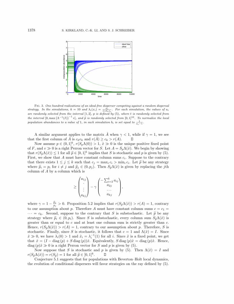
the strategy p = 1 cannot invade and displace the strategy !p. Hence, for a gen-eral "(x), we cannot expect that strategies of the form (5) will displace all otherstrategies. However, extensive simulations with the Beverton–Holt growth functions(i.e., !i(xi) = ai

1+bixi) suggest that the strategies given by (5) can displace any other

strategy (see Figure 3). Thus we make the following conjecture.Conjecture 5.1. If !i(xi) = ai

1+bixi, S is primitive and column stochastic, p is

given by (5), !p is not given by (5), and r(Sp"(0)) > 1, then

limn#$

Gn(x, y) = (x, 0)

whenever x > 0.Proof of Theorem 5.1 The key proposition (which gives us more than we need) is

the following.Proposition 5.2. Suppose that A is an irreducible nonnegative matrix with

column sums ci such that c1 = mini ci < maxi ci = ck. If !A is a nonnegative matrixobtained from A by changing its first column from

/

0001

a11

·...

ak1

2

3334to

/

0001

a11

·...

ak1

2

3334+ %

/

001

$5k

i=2 ai1a21

. . .ak1

2

334

for some positive % > 0, then r(A) < r(A). Alternatively, if A is a nonnegative matrixobtained from A by changing its last column from

/

0001

a1k

·...

akk

2

3334to

/

0001

a1k

·...

akk

2

3334$ %

/

001

$5k

i=2 aika2k

. . .akk

2

334

for some % ! (0, 1], then r(A) > r(A).Proof. Note that ck > r(A) > c1. Let wT be the left Perron vector for A such

that w1 = 1, and let v be the right Perron vector for A normalized so that wT v = 1.Observe that for any % such that A is nonnegative, A is irreducible and, consequently,v is a positive vector. Set W = diag (w1, . . . , wn). Then WAW&1 has all the columnsums equal to r(A). Consider the first column of WAW&1. We see that

a11 +k6

i=2

wiai1 = r(A) > c1 =k6

i=1

ai1.

Thus,

k6

i=2

wiai1 >k6

i=2

ai1.

It follows that r(A) = wT Av = wTAv + %v1($5k

i=2 ai1 +5k

i=2 wiai1) > wTAv =r(A).

1378 S. KIRKLAND, C.-K. LI, AND S. J. SCHREIBER

0 2000 4000 6000 8000 100000

1

2

3

4

5

6

7

8

time

met

apop

ulat

ion

abun

danc

e

ideal freeother

Fig. 3. One hundred realizations of an ideal-free disperser competing against a random dispersalstrategy. In the simulations, k = 10 and !i(xi) = ai

1+bixi. For each simulation, the values of ai

are randomly selected from the interval [1, 2], p is defined by (5), where t is randomly selected from

the interval [0,max,""1(I)

-"1v], and !p is randomly selected from [0, 1]10. To normalize the local

population abundances to a value of 1, in each simulation bi is set equal to 1ai"1 .

A similar argument applies to the matrix A when % < 1, while if % = 1, we seethat the first column of A is ckek and r(A) & ck > r(A).

Now assume p ! (0, 1]k, r(Sp"(0)) > 1, x ) 0 is the unique positive fixed pointof F , and v ) 0 is a right Perron vector for S. Let A = Sp"(x). We begin by showingthat r(S!p"(x)) ' 1 for all !p ! [0, 1]k implies that S is stochastic and p is given by (5).First, we show that A must have constant column sums ci. Suppose to the contrarythat there exists 1 ' j ' k such that cj = maxi ci > mini ci. Let !p be any strategywhere !pi = pi for i (= j and !pj ! (0, pj). Then S!p"(x) is given by replacing the jthcolumn of A by a column which is

&

/

0001

a1j

·...

akj

2

3334$ %

/

001

$5k

i=2 aija2j

. . .akj

2

334,

where % = 1 $ !pj

pj> 0. Proposition 5.2 implies that r(S!p"(x)) > r(A) = 1, contrary

to our assumption about p. Therefore A must have constant column sums c = c1 =· · · = ck. Second, suppose to the contrary that S is substochastic. Let !p be anystrategy where !pi ! (0, pi). Since S is substochastic, every column sum S!p"(x) isgreater than or equal to c and at least one column sum is strictly greater than c.Hence, r(S!p"(x)) > r(A) = 1, contrary to our assumption about p. Therefore, S isstochastic. Finally, since S is stochastic, it follows that c = 1 and "(x) = I. Sincex ) 0, we have !i(0) > 1 and xi = !&1

i (1) for all i. Since x is a fixed point, we getthat x = (I $ diag (p) + S diag (p))x. Equivalently, S diag (p)x = diag (p)x. Hence,diag (p)x ) 0 is a right Perron vector for S and p is given by (5).

Now suppose that S is stochastic and p is given by (5). Then "(x) = I andr(S!p"(x)) = r(S!p) = 1 for all !p ! [0, 1]k.

Conjecture 5.1 suggests that for populations with Beverton–Holt local dynamics,the evolution of conditional dispersers will favor strategies on the ray defined by (5).

EVOLUTION OF DISPERSAL 1379

Hence, it is natural to ask what happens when two strategies on this ray competeagainst one another.

Proposition 5.3. Assume that "(x) and S satisfy Assumptions A1–A4, !i(0) >1 for all i, and S is stochastic. Let p and !p be strategies given by (5) with t = d and

t = !d, where 0 < d < !d ' 1/max {,"&1(I)

-&1v}. Then the set of fixed points of G

are (0, 0) and

L = {(&x, (1 $ &)x : & ! [0, 1]},

where x = "&1(I)1. Moreover, if "(x) is continuously di!erentiable with !%i(xi) < 0

for all i, and ddxi

xi!i(xi) > 0 for all i, then there exists a neighborhood U + Rk+%Rk

+

of L and a homeomorphism h : [0, 1] %D " U with D = {z ! R2k&1 : /z/ < 1} suchthat h(&, 0) = &x + (1 $ &)x, h(0, D) = {(0, y) ! U}, h(1, D) = {(x, 0) ! U}, andlimn#$ Gn(x, y) = (&x, (1 $ &)x) for all (x, y) ! h({&}%D).

Proof. By the change of variables x #" "&1(I)&1diag (v)x, we can assume without

any loss of generality that p = d1 and !p = !d1. Thus, a point (x, y) > 0 is a fixedpoint of G if and only if

((1 $ d)I + dS)"(x + y)x = x,

((1 $ !d)I + !dS)"(x + y)y = y.

Since r(((1$ d)I + dS)"(x+ y))) = r((1$ !d )I + !dS)"(x+ y)) = 1 and d (= !d, Theo-rem 3.1 implies that "(x+ y) = I. Therefore, (x, y) needs to satisfy x+ y = "&1(I)1,

Sdx = dx, and S !dy = !dy. Since S is primitive, we get that x must be a scalar multipleof y. Hence, the fixed points of G are given by (0, 0) and L.

Now assume that x #" "(x) is continuously di!erentiable, !%i(x) < 0 for all i, and

ddxi

xi!i(xi) > 0 for all i. We will show that L is a normally hyperbolic attractor inthe sense of Hirsch, Pugh, and Shub [7]. Let (x, y) ! L. We have

DG(x, y) =

"Sd("%(x + y)diag (x) + "(x + y)) Sd"%(x + y)diag (x)

Sd"%(x + y)diag (y) Sd("%(x + y)diag (y) + "(x + y))

#.

Since 0 < !%i(xi + yi)(xi + yi) + !i(xi + yi) < !%

i(xi + yi)xi + !i(xi + yi) for all i, thediagonal blocks, Sd("%(x+y)diag (x)+"(x+y)) and Sd("%(x+y)diag (y)+"(x+y))of DG(x, y), are nonnegative primitive matrices. Since !%

i(xi+yi) < 0 for all i, the o!-diagonal blocks, Sd"%(x+y)diag (x) and Sd"%(x+y)diag (y), of DG(x, y) are negativescalar multiples of primitive matrices. Hence, DG(x, y) is a primitive matrix withrespect to the competitive ordering on Rk

+ % Rk+; i.e., (x, y) &K (x, y) if x & x and

y ' y. Since L is a line of fixed points, DG(x, y) has an eigenvalue of one associatedwith the eigenvector ("&1(I)1,$"&1(I)1). The Perron–Frobenius theorem impliesthat all the other eigenvalues of DG(x, y) are strictly less than one in absolute value.Hence, L is a normally hyperbolic one-dimensional attractor. Theorem 4.1 of [7]implies that there is a neighborhood U + Rk

+ % Rk+ of L and a homeomorphism

h : [0, 1]%D " U with D = {z ! R2k&1 : /z/ < 1} such that h(&, 0) = &x+(1$&)x,h(0, D) = {(0, y) ! U}, h(1, D) = {(x, 0) ! U}, and limn#$ Gn(x, y) = (&x, (1$&)x)for all (x, y) ! h({&}%D).

Proposition 5.3 implies that once a “resident” population playing a strategy ofthe form (5) has established itself, a “mutant” strategy of the form (5) can invadeonly in a weak sense: if the mutants enter at low density, deterministically they willconverge to an equilibrium with a low mutant density. After the invasion, one would

1380 S. KIRKLAND, C.-K. LI, AND S. J. SCHREIBER

expect that demographic or environmental stochasticity would with greater likelihoodresult in the displacement of the mutants. Hence, once a strategy of the form (5) hasestablished itself, it is likely to resist invasion attempts from other strategies of theform (5). Proposition 5.3 also suggests the following conjecture, which is supportedby simulations using the Beverton–Holt growth function.

Conjecture 5.2. Under the conditions of Proposition 5.3, for every (x, y) > 0there exists & ! [0, 1] such that

limn#$

Gn(x, y) = (&"&1(I)1, (1 $ &)"&1(I)1).

6. Discussion. For organisms that disperse unconditionally, we proved that aslower dispersing population competitively excludes a faster dispersing population.Similar results have been proven for reaction di!usion equations where the disper-sal kernel is self-adjoint [2], observed in a partial analysis of two patch di!erentialequations [8] and illustrated with simulations of two patch di!erence equations [17].Our proofs apply to di!erence equations with an arbitrary number of patches andwithout any symmetry assumptions about the dispersal matrix S. Since geographicaland ecological barriers often create asymmetries in the movement patterns of activedispersers and create asymmetries in abiotic and biotic currents that carry passivedispersers, accounting for these asymmetries is crucial and results in a significantlymore di#cult mathematical problem than the symmetric case. Theorem 3.1 providesthe solution to this problem by proving for any given environmental condition (i.e.,the choice of " and S), the principal eigenvalue for the growth dispersal matrix is adecreasing function of the dispersal rate. Hence, under all environmental conditions,populations that disperse more slowly spectrally dominate populations that dispersemore quickly. Despite this spectral dominance, simulations (e.g., Figure 1) illustratethat for appropriate initial conditions, faster dispersers can be numerically dominantas they initially spread across a landscape. This initial phase of numerical dominancehas empirical support in studies of northern range limits of butterflies: dispersal ratesincrease as species move north to newly formed favorable habitat [6]. Presumablyover a long period of time, selection will favor slower dispersal rates commensuratewith their ancestral rates of movement (R. Holt, personal communication). However,since all initial conditions do not lead to an initial phase of numerical dominance forthe faster dispersers (e.g., if the initial condition is a Perron vector for the slowerdisperser), we still require a detailed understanding of how the local intrinsic rates ofgrowth, the dispersal matrix, and initial conditions determine whether the faster orslower disperser is numerically dominant in the initial phase of establishment.

For conditional dispersers experiencing no dispersal costs (i.e., S is column stochas-tic and !i(0) > 1 for all i), we provide proofs that generalize previous findings in twopatch models [9, 17]. We prove that all dispersal strategies outside of a one-parameterfamily are not evolutionarily stable: when a population adopts one of these strategies,there are nearby strategies that can invade. For populations playing strategies in thisexceptional one-parameter family, the populations exhibit an ideal-free distribution atequilibrium: the per-capita growth rate is constant across the landscape [3]. Contraryto prior expectations [17], we show that are growth functions for which these ideal-freestrategies cannot displace all other strategies. However, numerical simulations withthe biologically plausible Beverton–Holt growth functions suggest that populationsplaying these ideal-free strategies can displace populations playing any other strat-egy. Moreover, when a population at equilibrium plays an ideal-free strategy, we provethat a population playing another ideal-free strategy cannot increase from being rare

EVOLUTION OF DISPERSAL 1381

and, consequently, is likely to be driven to extinction by stochastic forces. For popula-tions playing these ideal-free strategies, the dispersal likelihood in a patch is inverselyproportional to the equilibrium abundance in a patch. Hence, enriching one patchmay result in the evolution of lower dispersal rates in that patch. Conversely, habitatdegradation of a patch may result in the evolution of higher dispersal rates in thatpatch. These predictions about ideal-free strategies, however, have to be viewed withcaution, as they are sensitive to the assumption of no dispersal costs. The inclusion ofthe slightest dispersal costs destroys this one-parameter family of evolutionary stablestrategies and leaves only the nondispersal strategy as a candidate for an evolutionarystable strategy.

Our models make several simplifying assumptions, and relaxing these assumptionsprovides several mathematical problems of biological interest. Most importantly, ourmodels do not include temporal heterogeneity, which is an important ingredient inthe evolution of dispersal [17]. Temporal heterogeneity can be generated exogenouslyor endogenously and when combined with spatial heterogeneity can promote the evo-lution of faster dispersers [10, 13, 17]. For instance, Hutson, Mischaikow, and Polacik[13] proved that a faster disperser can displace or coexist with a slower disperser forperiodically forced reaction di!usion equations. Whether similar results can be provenfor periodic or, more generally, random di!erence equations requires answering math-ematically challenging questions about spectral properties of periodic and randomproducts of nonnegative matrices. Similar challenges arise when replacing increasinggrowth functions with unimodal growth functions [4, 10, 19] that can generate tem-poral heterogeneity via periodic and chaotic population dynamics.

Acknowledgments. The authors thank participants of the William and Mary“matrices in biology sessions” for their valuable feedback on this evolving work. Inparticular, we thank Greg Smith and Marco Huertas for finding counterexamples toan earlier conjectured form of Theorem 3.1. We also thank Bob Holt, Vivian Hutson,Konstantin Mischaikow, and an anonymous referee for their encouraging commentsand helpful suggestions.

REFERENCES

[1] R. J. H. Beverton and S. J. Holt, On the Dynamics of Exploited Fish Populations, Fish.Invest. Ser. II 19, Ministry of Agriculture, Fisheries and Food, London, UK, 1957.

[2] J. Dockery, V. Hutson, K. Mischaikow, and M. Pernarowski, The evolution of slowdispersal rates: a reaction di!usion model, J. Math. Biol., 37 (1998), pp. 61–83.

[3] S. D. Fretwell and H. L. Lucas, On territorial behavior and other factors influencing patchdistribution in birds, Acta Biotheoretica, 19 (1970), pp. 16–36.

[4] W. M. Getz, A hypothesis regarding the abruptness of density dependence and the growth rateof populations, Ecology, 77 (1996), pp. 2014–2026.

[5] A. Hastings, Can spatial variation alone lead to selection for dispersal?, Theor. Pop. Biol.,24 (1983), pp. 244–251.

[6] J. K. Hill, C. D. Thomas, R. Fox, M. G. Telfer, S. G. Willis, J. Asher, and B. Huntley,Responses of butterflies to twentieth century climate warming: Implications for futureranges, Roy. Soc. Lond. Proc. Ser. Biol. Sci., 269 (2002), pp. 2163–2171.

[7] M. W. Hirsch, C. C. Pugh, and M. Shub, Invariant Manifolds, Springer-Verlag, Berlin, 1977.[8] R. D. Holt, Population dynamics in two-patch environments: Some anomalous consequences

of an optimal habitat distribution, Theor. Pop. Biol., 28 (1985), pp. 181–208.[9] R. D. Holt and M. Barfield, On the relationship between the ideal-free distribution and the

evolution of dispersal, in Dispersal, J. Clobert, E. Danchin, A. Dhondt, and J. Nichols,eds., Oxford University Press, Oxford, UK, 2001, pp. 83–95.

[10] R. D. Holt and M. A. McPeek, Chaotic population dynamics favors the evolution of dispersal,Amer. Nat., 148 (1996), pp. 709–718.

1382 S. KIRKLAND, C.-K. LI, AND S. J. SCHREIBER

[11] S. B. Hsu, H. L. Smith, and P. Waltman, Competitive exclusion and coexistence for compet-itive systems on ordered Banach spaces, Trans. Amer. Math. Soc., 348 (1996), pp. 4083–4094.

[12] V. Hutson, S. Martinez, K. Mischaikow, and G. T. Vickers, The evolution of dispersal,J. Math. Biol., 47 (2003), pp. 483–517.

[13] V. Hutson, K. Mischaikow, and P. Polacik, The evolution of dispersal rates in a heteroge-neous time-periodic environment, J. Math. Biol., 43 (2001), pp. 501–533.

[14] V. S. Ivlev, Experimental Ecology of the Feeding of Fishes, Yale University Press, New Haven,CT, 1955.

[15] M. L. Johnson and M. S. Gaines, Evolution of dispersal: Theoretical models and empiricaltests using birds and mammals, Annu. Rev. Ecol. Syst., 21 (1990), pp. 449–480.

[16] S. A. Levin, D. Cohen, and A. Hastings, Dispersal strategies in patchy environments, The-oret. Pop. Biol., 26 (1984), pp. 165–191.

[17] M. A. McPeek and R. D. Holt, The evolution of dispersal in spatially and temporally varyingenvironments, Amer. Nat., 6 (1992), pp. 1010–1027.

[18] K. Mischaikow, H. Smith, and H. R. Thieme, Asymptotically autonomous semiflows: Chainrecurrence and Lyapunov functions, Trans. Amer. Math. Soc., 347 (1995), pp. 1669–1685.

[19] W. E. Ricker, Stock and recruitment, J. Fish. Res. Board. Can., 11 (1954), pp. 559–623.[20] A. L. Shanks, Mechanisms of cross-shelf dispersal of larval invertebrates and fish, in Ecology

of Marine Invertebrate Larvae, CRC, Boca Raton, FL, 1995, pp. 324–367.