On the Existence of Best Mitscherlich, Verhulst, and WestGrowth Curves for Generalized Least-Squares Regression

Yves Nievergelt

Department of Mathematics, Eastern Washington University, Cheney, WA 99004-2418, USA

Abstract

Practical difficulties arise in fitting Mitscherlich, Verhulst, or West growth curves todata. Obstacles include divergent iterations, negative values for theoretically positiveparameters, or the absence of any best-fitting curve. An analysis reveals that such ob-stacles occur near removable singularities of the objective function to be minimized forthe regression. Such singularities lie at the transition to different types of curves, in-cluding exponentials, hyperbolae, lines, and step functions. Removing the singularitiesfits all such curves into a connected compactified topological space, which guaranteesthe existence of a global minimum for the continuous objective function, and whichalso provides a smooth and transparent transition from one type of curve to another.

Keywords: Growth curves, parameter identification, singular covariance, weightednonlinear least squares2000 MSC: 41A27,41A28,41A30,41A63,65D10,65K10,80A30,92C45,92D25

0. Introduction

This article determines the existence, or the absence, of “best” shifted exponentialcurves (1), called Mitscherlich’s laws, relative to weighted or generalized (correlated)least squares. Also called asymptotic regression [43], [47], [54], the problem consists infitting to data points (t1, q1), . . . , (tN , qN ) the parameters A, B, and C in equation (1):

q = A · eC·t +B. (1)

Equation (1) describes all phenomena modeled by the first-order linear differentialequation

dq

dt= C · (q −B) (2)

with constant coefficients B and C 6= 0, and hence also by Bernoulli equations [51, p.58–59]. For instance, West’s recent model of ontogenetic growth of organisms [62],

dm

dt= a · (m3/4 −m/M1/4), (3)

Email address: ynievergelt@ewu.edu (Yves Nievergelt)

Preprint submitted to Journal of Computational and Applied Mathematics May 3, 2013

is a Bernoulli equation, which reduces to equation (2) for q := m1/4:

d

dt(m1/4) =

−a4 ·M1/4

· (m1/4 −M1/4), (4)

with B = M1/4 and C = −a/(4 ·M1/4), or M = B4 and a = −4 · B · C. Thesolution

m1/4(t) = M1/4 + (m1/40 −M1/4) · ea·(t0−t)/(4·M

1/4) (5)

is Mitscherlich’s law (1) with A = (m1/40 −M1/4) · ea·t0/(4·M1/4), or m1/4

0 = A ·e−C·t0 + B. If A,B, q > 0, then K := 1/B, D := ln(A/B), and y := 1/q give aVerhulst curve (6):

y =K

1 + eD+C·t . (6)

Applications of Mitscherlich, West, and Verhulst curves (1), (5), and (6) include, forinstance,

1. agronomy, to evaluate and optimize the efficiency of fertilizers [47], [54];2. chemical kinetics [24, p. 20, eq. (29)], [31, p. 993], [36, p. 65], [41], [42], [46, p.

393, eq. (1)], to identify the type of chemical reaction occurring in experiments;3. population growth [4], [5], [13], [61], [25], [30], [33], [44], [49], [52], [59], [60];4. physiology, to model the growth over time of plants and animals [50], [62], or

individual organs, for example, wing span [23, p. 808];5. rheology [15].

Hence arises the need to estimate the parameters A, C, and B or K, that fit the databest relative to generalized (ordinary, weighted, or correlated) least squares [58]. Gen-eral theorems already provide sufficient conditions on the monotonicity and convexityof the data for the existence of a weighted least-squares Mitscherlich curve [21] ornecessary and sufficient conditions for a weighted least-squares Verhulst curve [29].Examples show that there are data that fail to satisfy the hypotheses of such theoremsand for which no best-fitting curves exist [9], [10], [11], [21]. Alternatively, computedsolutions yield negative values for theoretically positive parameters:

A successful fit results in positive values for [K] and [−C] but data whichdeviate too far from the model result in either a fit to a curve with a negative[K] or negative [−C] [33, p. 94, § 2].

The present shows that such situations reflect features of the modeled phenomenon.For instance, replacing the Verhust equation (6) by the modeling differential equation

dy

dt=

C

K· y · (K − y), (7)

L. J. Reed and J. Berkson [49, p. 765] had already pointed out that the solution curvey becomes a hyperbola if A · B < 0 and C/K remains constant while K tends to0, though they did not mention the possibility that the solution becomes a Malthusian

2

[35, II.7] exponential growth curve as K diverges to +∞. In either case C/K neednot remain constant but need only converge to a limit. A similar situation occurs as Atends to 0. Neither did Reed and Berkson [49] mention why or how parameters woulddiverge, converge to anything, or change in the first place. Indeed, they selected thetype of curve to be fitted before starting the regression, which never failed for theirexamples [49, p. 769–779]. The present analysis shows that the limits happen to lieexactly at a removable singularity of the objective function for the generalized least-squares regression.

Specifically, the present work first extends the literature from weighted to poten-tially correlated least squares with potentially non-invertible covariance matrices, sec-ond reveals that the correlated least-squares objective function extends analytically tothe special case of straight lines and continuously to step functions, and third extendssuch results to West’s ontogenetic growth curves.

The strategy adopted here consists of fixing one parameter, C for Mitscherlich’slaw (1), and in analyzing the explicit formulae for the solutions of the generalizedlinear least-squares regression with the other two parameters, A and B, in terms of thefixed parameter C.

To this end, Sections 1 and 2 are akin to [22, Ch. 4] but extended to generalizedleast squares with semi scalar-products. Section 1 summarizes motivations for gen-eralized least squares from probability or statistics. Section 2 summarizes solutionsfor generalized least squares using only linear algebra, without probability or statis-tics. Section 3 applies the previous sections to regressions for Mitscherlich’s law (1)parametrized by C. Using [64], Section 4 generalizes the previous sections further tohandle singular covariance matrices. Section 5 establishes sufficient criteria for a best-fitting Mitscherlich’s law (1) to be the reciprocal of a Verhhulst curve (6). Section 6presents examples with real data.

1. Notation for Generalized Least-Squares

Though the numerical solution of least-squares problems proceeds more accuratelywith other algorithms [6], [18], [32], the present analysis and resolution of singularitiesuses explicit formulae for the solutions. Moreover, examples from Section 6 show thatthe data may be highly correlated, in the sense that in the covariance matrix entriesare larger off than on the diagonal. To allow for such correlations, the present analysisallows for a generalized regression, which arises in fitting a least-squares line to data(x1, y1), . . ., (xN , yN ) in the plane as described in [20, p. 35–42 & 112–114]. Specif-ically, each point (xk, yk) may be the average of repeated measurements (xk, yk,1). . ., (xk, yk,Mk

), with the same absissa xk but different ordinates yk,1, . . ., yk,Mkwith

mean yk = (yk,1 + · · ·+yk,Mk)/Mk. Consequently, the measurements yk,1, . . ., yk,Mk

are modeled as values of a random variable Yk with expectation EYk. The random vari-ables Y1, . . . , YN may be correlated with a symmetric nonnegative covariance matrixV defined by [16, § 22.3]

Vk,` = E [(Yk − EYk) · (Y` − EY`)].

A linear model for such data consists of N linear equations Yk = A · xk + B + εk,where each εk is a random variable with Eεk = 0. With the column vectors ~P =

3

(A,B)′, ~Y = (Y1, . . . , YN )′, ~x = (x1, . . . , xN )′, ~0 = (0, . . . , 0)′, ~1 = (1, . . . , 1)′, ~ε =(ε1, . . . , εN )′, where ′ denotes transposition, and with the design matrix X = (~x,~1),the model becomes

~Y = X · ~P + ~ε.

The problem consists of estimating the vector of parameters ~P . A linear transforma-tion into uncorrelated variables simplifies matters. To this end, assume first that V isinvertible, and let T be any matrix such that T ′ · T = V −1, so that V = T−1 · (T−1)′,and define

~Z = T · ~Y .

Under the hypothesis of a vanishing expectation Eε = ~0, the random vector ~Z hasexpectation

E ~Z = T · E ~Y = T ·X · ~P

and covariance matrix T · V · T ′ = I [27, p. 410, ex. 12.4]. With the Euclideannorm ‖~p‖2 defined by ‖~p‖22 = ~p′ · ~p, a best linear unbiased estimate of the vector ofparameters ~P = (A,B)′ is a solution ~P∗ = (A∗, B∗)′ minimizing the objective [48, §3.3], [57, p. 144]

L(~P ) := ‖T ·X · ~P − T · ~y‖22 = (X · ~P − ~y)′ · T ′ · T · (X · ~P − ~y). (8)

The literature formulates the generalized least-squares solution ~P∗ = (A∗, B∗)′ fromthe normal equations in terms of (X ′T ′TX)−1 or with pseudo-inverses [1], [6, p. 7],[20, p. 108–116], [32, p. 37], [48, p. 47–50], [55, p. 5], [56, p. 246], but here adifferent notation, elaborating on [12], [34, p. 209], is convenient to track solutions asparameters change. The derivations hold not only for V −1, but also for any symmetricnonnegative semi-definite generalized inverse V −, defined as any matrix such that V ·V − · V = V , and any matrix T such that T ′ · T = V − [64, p. 1194] and T ·~1 6= ~0. (IfT ·~1 = ~0, then T ·X · ~P = T · ~x ·A+~0 ·B in the objective (8), so that B cannnot beestimated). Thus T defines a semi scalar-product

〈~p, ~q〉 := ~p′ · T ′ · T · ~q (9)

and an induced semi-norm ‖~p‖2 := 〈~p, ~p〉 [63, p. 250 & p. 23], which reduce general-ized least squares to ordinary least squares: for all sequences ~p, ~q ∈ RN , re-define theirmean meanT (~p), variance varT (~p), covariance covT (~p, ~q), and correlation coefficientcorT (~p, ~q) by

meanT (~p) :=〈~p,~1〉〈~1,~1〉

=~p′ · T ′ · T ·~1~1′ · T ′ · T ·~1

, (10)

covT (~p, ~q) :=〈~p−meanT (~p) ·~1, ~q −meanT (~q) ·~1〉

〈~1,~1〉, (11)

varT (~p) := covT (~p, ~p), (12)

corT (~p, ~q) :=covT (~p, ~q)√

varT (~p) · varT (~q). (13)

4

For each finite squence ~p, define the centered sequence by p := ~p−meanT (~p) ·~1. Thefollowing identities will then lead to further simplifications:

meanT (~1) :=〈~1,~1〉〈~1,~1〉

= 1, (14)

meanT (p) =〈~p−meanT (~p) ·~1,~1〉

〈~1,~1〉= meanT (~p)−meanT (~p) = 0. (15)

2. Solutions for Generalized Least-Squares

With the Euclidean inner product replaced by the semi scalar-product (9) defined byT , the same calculations as for ordinary least squares show that the line of generalizedleast squares, which minimizes the objective (8), passes through the generalized mean(meanT (x),meanT (y)) defined by formula (10). Algebra gives the following solution,with all formulae gathered here at the same place:

A∗ =〈~y −meanT (~y) ·~1, ~x−meanT (~x) ·~1, 〉〈~x−meanT (~x) ·~1, ~x−meanT (~x) ·~1, 〉

=covT (~x, ~y)

varT (~x); (16)

B∗ = meanT (~y)−A∗ ·meanT (~x); (17)y = A∗ · [x−meanT (~x)] + meanT (~y). (18)

L(A∗) = 〈~1,~1〉 · varT (~y) ·[1− corT (~x, ~y)2

]. (19)

3. Asymptotic Generalized Least-Squares Regression

This section focuses on fitting to data the parametersA, B, and C of Mitscherlich’slaw (1), including the limiting cases where C either tends to 0 or diverges to ±∞,subject to the following standing hypotheses.

Hypotheses 1. With R denoting the set of all real numbers, the present theory pertainsto a weight matrix T ∈ RN×N and data points (tk, qk) for k ∈ {1, . . . , N} such that

(1.1) qk > 0 for every k ∈ {1, . . . , N};

(1.2) there exist k, ` ∈ {1, . . . , N}, with tk 6= t`; in particular, N ≥ 2;

(1.3) for all k, ` ∈ {1, . . . , N}, if k < `, then tk ≤ t`, so that t1 ≤ · · · ≤tN ;

(1.4) T depends continuously on the parameter C ∈ [−∞,+∞], with T ·~1 6= ~0.

Defining a generalized Mitscherlich law to be a Mitscherlich law, or a line, or astep function, leads to the main result.

Theorem 2. For each data set satisfying hypotheses 1 there exists a generalized least-squares generalized Mitscherlich law.

5

Proof. The proof forms the object of the present section. Subsections 3.1, 3.2, and 3.3show that the objective (26) has a continuous extension, also denoted by F , to theextended real line [−∞,+∞] with the topology of the two-point compactification.Consequently, F has a global minimum.

In applications, if the covariance matrix V is invertible, then the weight matrix Tcan be any constant matrix such that T ′ ·T = V −1. If V is not invertible, however, thenT is not constant but depends on C ∈ [−∞,+∞] in a specific way, as explained inSection 4. Nevertheless, the denominator 〈~1,~1〉 = ~1′ · T ′ · T ·~1 > 0 remains boundedaway from 0 by uniform continuity on the compact interval [−∞,+∞]. Therefore,to simplify notation, Sections 3, 4, and 5 use the notation T instead of TC and 〈 , 〉instead of 〈 , 〉TC

.A common method for fitting Mitscherlich’s law (1) to data proceeds by unweighted

non-linear least-squares regression [43, p. 328], [47, p. 499], [54, p. 250], minimizing

F (A,B,C) :=N∑k=1

(A · eC·tk +B − qk

)2. (20)

Its Hessian matrix has been derived in the literature [54, p. 250, eq. (2.3)], but F hasa singularity, hitherto seemingly unnoticed, along the planes where A = 0 or C = 0,where its Hessian matrix is singular. To remove the singularity, define the change ofvariable

xCk := eC·tk . (21)

With the notation ~xC := (xC1 , . . . , xCN )′ and a weight matrix T , the objective (20)

becomes

F (A,B,C) :=∥∥∥∥T · [(~xC ,~1) ·

(AB

)− ~q]∥∥∥∥2

2

. (22)

Then for each rate C 6= 0 the regression amounts to a linear regression for qk versusxCk . AsC tends to 0, so does the smallest singular value ofXC := (~xC ,~1); the pseudo-inverse X†C becomes unbounded and consequently need not be a continuous functionof the entries of XC [32, p. 44]. Thus the shortest least-squares solution does notremove this singularity. Several cases can arise, according to the values of C, limC→0,limC→+∞, and limC→−∞.

3.1. Finite Non-Zero Growth RateIf C 6= 0, then xCk 6= xC` for some k and `, whence varT (xC) > 0 by hypothe-

sis (1.2). Formulae (16) – (18) in Section 2 withX = (~xC ,~1) then yield the generalizedleast-squares line with slope AC and intercept BC in the form

AC =covT (~xC , ~q)

varT (~xC), (23)

BC = meanT (~q)−AC ·meanT (~xC), (24)q = meanT (~q) +AC ·

[xC −meanT (~xC)

]. (25)

6

Substituting formulae (23) and (24) back into the objective function (22) gives an ob-jective function F of the single variable C analogous to the objective function (8):

F (C) := L(AC) =∥∥∥T · {AC · [~xC −meanT (~xC) ·~1

]−[~q −meanT (~q) ·~1

]}∥∥∥2

2.(26)

Closed-form formulae for a solution C to F ′(C) = 0, if any, seem elusive: alreadyfor the special case of N = 4 equally spaced abscissae, and with T = I , the equationF ′(C) = 0 is a polynomial equation of degree 6 in z := eC [47, p. 499]. Nevertheless,Subsections 3.2 and 3.3 show that F has a continuous extension to the compact interval[−∞,+∞], which guarantees the existence of at least one global minimum.

3.2. Growth Rate Near ZeroIf C = 0, then xCk = 1 = xC` for all k and `, whence the variance of xC vanishes.

For C near 0 but C 6= 0, Subsection 3.1 applies; with o(h) or O(h) denoting any termsuch that limh→0 o(h)/h = 0 or limh→0O(h) = 0, formula (21) leads to

xCk − 1C

=eC·tk − 1

C=

M∑j=1

Cj−1 ·tjkj!

+O(CM ), (27)

xCk −meanT (~xC)C

=xCk − 1C

−meanT

(~xC − 1C

)= tk −meanT (~t) +O(C).(28)

Substituting formulae (27) and (28) into formula (23) and algebra gives

limC→0

AC · [xC −meanT (~xC)] =covT (~t, ~q)

varT (~t)· [t−meanT (~t)] = A∗ · [t−meanT (~t)].(29)

Thus formulae (25) and (29) show that the fitted equation (25) converges to the line ofgeneralized linear least squares for q versus t:

limC→0

q = meanT (~q) +A∗ · [t−meanT (~t)]. (30)

Also, substituting the same limit (29) back into formula (26) for the objective showsthat

limC→0

F (C) = 〈~1,~1〉 · varT (~q) ·[1− corT (~t, ~q)2

], (31)

which also reproduces equation (19). Consequently, F has an analytic extension, alsodenoted by F , across C = 0, where the regression seamlessly fits the least-squares linewith equation

q = A∗ · t+B∗, (32)

or, equivalently, the hyperbola with equation y = 1A∗·t+B∗ , explaining one of Reed and

Berkson’s special cases [49, p. 765]. In the case with A∗ = 0 6= B∗, this hyperbolaalso includes the straight horizontal line y = 1/B∗, which also corresponds to A = 0in y = K/(1 +A · eC·t).

7

3.3. Growth Rate Diverging to InfinityForC diverging to +∞, factoring out the largest term xCN in formulae (21) and (23)

gives limC↗+∞AC · eC·t = 0 and limC↗+∞AC · xCk = 0 for t < tN and 1 ≤ k ≤N − 1. For k = N , define the temporary abbreviation

LN := limC↗+∞

meanT (~xC)xCN

= limC↗+∞

1xCN· 〈~x

C ,~1〉〈~1,~1〉

=〈~eN ,~1〉〈~1,~1〉

. (33)

Hence the limit (33) combined with equation (15) and more algebra leads to

limC↗+∞

AC · [xCN −meanT (~xC)] =〈~q −meanT (~q)~1, ~eN 〉

〈~eN , ~eN 〉. (34)

Therefore formulae (26) and (34) show that limC↗+∞ F (C) exists. To show that thelimiting fitted curve is a step function, split each ~v ∈ RN in the form ~v = v+ vN · ~eN .Thus

meanT (~q) =〈~q,~1〉〈~1,~1〉

=〈q + qN · ~eN ,~1〉

〈~1,~1〉=〈q,~1〉〈~1,~1〉

+ qN ·〈~eN ,~1〉〈~1,~1〉

. (35)

At t := tN ,

limC↗+∞

q(tN ) = limC↗+∞

{meanT (~q) +AC ·

[eC·tN −meanT (~xC)

]}(36)

= meanT (~q) +〈~q −meanT (~q)~1, ~eN 〉〈~eN − LN~1, ~eN − LN~1〉

· 〈~1− ~eN ,~1〉〈~1,~1〉

(37)

= qN +〈q −meanT (~q)1, ~eN 〉

〈~eN , ~eN 〉6= qN

except if 〈~ek, ~e`〉 = δk,`, or q1 = · · · = qN , by equation (34). For t < tN ,

limC↗+∞

q(t) = limC↗+∞

meanT (~q) +AC ·[eC·t −meanT (~xC)

](38)

= meanT (~q) + 0− 〈~q −meanT (~q)~1, ~eN 〉〈~eN − LN~1, ~eN − LN~1〉

· 〈~eN ,~1〉

〈~1,~1〉. (39)

If 〈~q − meanT (~q)~1, ~eN 〉 6= 0, then the values (37) and (39) differ from each other,because if 〈~1 − ~eN ,~1〉 = −〈~eN ,~1〉, then adding 〈~eN ,~1〉 to both sides yields ‖~1‖2 =〈~1,~1〉 = 0. Thus the fitted curve consists of a straight horizontal half-line on ]−∞, tN [and a point at tN .

Substituting equation (35) into (39) shows that the coefficient of qN vanishes, sothat

limC↗+∞

q = meanT (q) + 0− 〈q −meanT (q)~1, ~eN 〉〈~eN − LN~1, ~eN − LN~1〉

· 〈~eN ,~1〉

〈~1,~1〉. (40)

Similar results hold as C diverges to −∞. Substituting formulae (36)–(37) and (38)–(39) in formula (26) shows that F extends continuously to [−∞,+∞].

8

4. Fitting Mitscherlich Curves with Singular Covariance Matrices

The preceding considerations apply to any weight matrix T ∈ RN×N with T ·~1 6=~0. Specific choices for T lead to specific features of the solutions. For instance, if thecovariance matrix V of the data is invertible, then for each C the solutions AC and BCare best linear unbiased estimators of A and B if and only if T ′ · T = V −1. However,“singular covariance matrices arise naturally in certain important classes of statisticalproblems” [64, p. 1190–1191]. If V is singular, then the solutions are best linearunbiased estimators if and only if T ′ · T = V − is a generalized inverse of V , whichmeans that V · V − · V = V , with the additional condition that V · (V −)′ projects therange ofX ,R(X), ontoR(X)∩R(V ) [64, p. 1193]. This section shows that for someapplications there is such a matrix T depending continuously on C ∈ [−∞,+∞].

The foregoing conditions on T can be met with a positive definite matrix T ′ · T , sothat T ·~1 6= ~0, as follows [64, p. 1194, eq. (3.6)]. Let the Singular-Value Decompositionof V be

V = U · Σ · U ′ =(U1 U0

)·(D 00′ 0

)·(U ′1U ′0

), (41)

where U = (U1, U0) ∈ RN×N is orthogonal, U1 ∈ RN×r spans R(V ), U0 ∈RN×(N−r) spans the nullspace N (V ), and D = diagonal(σ1, . . . , σr) ∈ Rr×r is pos-itive definite diagonal. Following [64, p. 1193], extend any basis S forR(X) ∩R(V )to any basis (S,R) ofR(X):

(S,R) =(U1 U0

)·(A B1

0 B0

),

where A ∈ Rr×k, B1 ∈ Rr×`, B0 ∈ R(N−r)×`. There is a matrix K ∈ Rr×(N−r)

with B1 = K · B2, and hence V · (V −)′ · R = 0 [64, p. 1193]. Define a non-singularmatrix T by

T =(D−1/2 −D−1/2 ·K

0 I

)· U ′. (42)

4.1. Ranges Allowing for Constant Weight MatricesIfR(X) ⊆ R(V ), then S = X = (~xC ,~1),R = ∅,K = 0, and T = diagonal(D−1/2, I)·

U ′. This situation contains the case where V is invertible, because thenR(X) ⊆ RN =R(V ). If X = (~xC ,~1) andR(X) 6⊆ R(V ) withR(X)∩R(V ) 6= {~0} but ~1 /∈ R(V ),so that r < N , then R = ~1 ∈ RN and K = (~1r, 0) ∈ Rr×(N−r) with ~1r ∈ Rrand 0 ∈ Rr×[(N−r)−1] work. The preceding sections then apply verbatim because Tremains constant, independent of C.

4.2. Complementary RangesFor some applicationsR(X)⊕R(V ) = RN so thatR(X) ∩R(V ) = {~0} but the

columns of (X,V ) form a basis of RN . Thus S = ∅ and

R = X =(~xC ~1

)=(U1 U0

)·(B1

B0

). (43)

9

From equation (43) and U ′ ·U = I follow the equationsB1 = U ′1 ·X andB0 = U ′0 ·X:(U ′1 ·

(~xC ~1

)U ′0 ·

(~xC ~1

) ) =(U ′1U ′0

)·(~xC ~1

)=(B1

B0

). (44)

Also, B0 = U ′0 · X is invertible because (U1, U0)′ · (V,X) is invertible and blockupper triangular with the lower right-hand block U ′0 ·X . Thus K := B1 · B−1

0 solvesB1 = K · B0. The design matrix X = (~xC ,~1) with U1 = (~u1, . . . , ~uN−2) andU0 = (~uN−1, ~uN ) leads to

B1 =

~u′1 · ~xC ~u′1 ·~1...

~u′N−2 · ~xC ~u′N−2 ·~1

, B0 =(~u′N−1 · ~xC ~u′N−1 ·~1~u′N · ~xC ~u′N ·~1

).

Ki,j = (B1 ·B−10 )i,j =

~u′i · ~xC · ~u′N+1−j ·~1− ~u′N+1−j · ~xC · ~u′i ·~1~u′N−1 · ~xC · ~u′N ·~1− ~u′N · ~xC · ~u′N−1 ·~1

. (45)

If alsoR(~t,~1)⊕R(V ) = RN , then again U ′0 · (~t,~1) is invertible. As in Subsection 3.2,the limited development ~xC = ~1+C ·~t+o(C ·~t) shows thatK converges, and hence sodoes T , as C tends to 0, to the values ofK and T for the linear least-squares regressionwith data (t1, q1), . . . , (tN , qN ) and covariance matrix V :

limC→0

Ki,j = limC→0

(B1 ·B−10 )i,j =

~u′i · ~t · ~u′N+1−j ·~1− ~u′N+1−j · ~t · ~u′i ·~1~u′N−1 · ~t · ~u′N ·~1− ~u′N · ~t · ~u′N−1 ·~1

.(46)

As in Subsection 3.3, for C diverging to +∞, factoring out the largest term xCN =eC·tN shows that xCk /x

CN = eC·(tk−tN ) tends to 0 for tk < tN while xCN/x

CN = 1, so

that ~xC/xCN tends to ~eN . If R(~eN ,~1) ⊕ R(V ) = RN , then U ′0 · (~eN ,~1) is invertible,and Ki,j tends to

limC→+∞

Ki,j =~u′i · ~eN · ~u′N+1−j ·~1− ~u′N+1−j · ~eN · ~u′i ·~1~u′N−1 · ~eN · ~u′N ·~1− ~u′N · ~eN · ~u′N−1 ·~1

. (47)

Thus although B−10 diverges as C tends to 0 or ±∞, equations (45) and (47) show

that K is continuous on [−∞,+∞], so that T also converges and remains invertibleby formula (42).

5. Sufficient Criteria for Weighted Least-Squares Mitscherlich Curves to Be ofSpecific Types

In applications, coefficients with different signs may reflect different phenomena[49]. Yet highly correlated data may switch the signs of fitted coefficients [39]. There-fore, this section focuses only on uncorrelated data to establish sufficient criteria forweighted least-squares Mitscherlich curves to have parameters A, B, and C with spe-cific signs. The relevant feature of uncorrelated weighted least-squares is that with a

10

diagonal matrix T ′ · T the objectives (8) and (22) are monotonic increasing functionsof each residual |A · eC·tk + B − qk|. Consequently, to prove that a curve M† fits thedata better than a curve M‡ does, it suffices to prove that M† lies between M‡ and thedata, defined to mean that qk ≤ M†(tk) ≤ M‡(tk) or qk ≥ M†(tk) ≥ M‡(tk), so that|M†(tk) − qk| ≤ |M‡(tk) − qk| for every k ∈ {1, . . . , N}. Thus the results hold notonly for weighted least squares, but also for objectives that are weighted `p-norms ofthe residuals, with 2 replaced by any p ≥ 1 in formula (22).

5.1. Sufficient Criteria for Weighted Least-Squares Lines to Have Positive Slopes

Because the least-squares regression objective (22) is linear relative to A and B,criteria for the signs of the coefficients rely on the signs of the slope and interceptof least-squares lines. In this subsection the proofs are omitted because they involvemostly straightforward algebra. Theorem 3 and formula (16) confirm that for uncorre-lated data the weighted least-squares line has a positive slope for increasing data, anda negative slope for decreasing data. (Theorem 3 fails with correlated data: the fittedslope may have the opposite sign [39].)

Theorem 3. If T ′ · T is diagonal and invertible, and if the finite sequences ~x and ~y aremonotonic, either both non-decreasing, or both non-increasing, then covT (~x, ~y) ≥ 0.

If ~x or ~y is non-decreasing while the other is non-increasing, then covT (~x, ~y) ≤ 0.Equality holds if and only if at least one of ~x or ~y is constant.

Theorem 5 shows that for convex or concave data, weighted least-squares linescross the polygonal function interpolating the data exactly twice, whence for convexdata weighted least-squares Mitscherlich curves cannot be concave. Definition 4 spec-ifies these concepts.

Definition 4. For all data z1 = (x1, y1), . . . , zN = (xN , yN ) with x1 < · · · < xNand N ≥ 3, let Ψ be the piecewise affine function interpolating all the data, so thatΨ(xk) = yk for every k ∈ {1, . . . , N} and Ψ is affine on [xk, xk+1] for every k ∈{1, . . . , N − 1}, extended affinely from [xN−1, xN ] to [xN−1,+∞[, and from [x1, x2]to ]−∞, x1]. The data are convex or super-linear (respectively concave or sub-linear)if and only if no triples of data points are collinear and Ψ is weakly convex (respectivelyconcave).

Theorem 5. If T ′·T is diagonal and invertible, and if the data z1 = (x1, y1), . . . , zN =(xN , yN ) with x1 < · · · < xN are convex, then the weighted least-squares line L in-tersects the piecewise affine interpolating function Ψ (from Definition 4) exactly twice.

Also, for each concave funtion Λ such that the complement of its graph R2\Λ splitsinto two disjoint connected components, there is a line between Λ and the data. Hencethe weighted least-squares line L fits the data better than any such concave funtion Λdoes.

Theorem 5 also fails with correlated data: a line fitted to increasing and convex datamay have a negative slope and intersect the polygonal interpolating function only once[39].

11

5.2. Sufficient Criteria for Weighted Least-Squares Mitscherlich Curves Not to Be StepFunctions

Subsection 3.3 shows that as the rate C diverges to ±∞ the generalized least-squares Mitscherlich curves fitted to the data tend to step functions. For uncorrelatedmonotonic data, however, this subsection shows that weighted least-squares Mitscher-lich curves are not step functions. In this subsection the proofs involve mostly straight-forward algebra and are omitted. Theorem 6 shows that for weighted least squares thefitted step function begins or ends at the first or last data point as C diverges to −∞ or+∞.

Theorem 6. If T ′ · T is diagonal, and if C diverges to +∞ (respectively −∞),then the weighted least-squares Mitscherlich curves minimizing the objective (26) con-verge on ] − ∞, tN ] (respectively [t1,+∞[) to a step function that passes throughzN = (tN , qN ) (respectively z1) and coincides with the weighted least-squares con-stant horizontal line for the remaining data over ]−∞, tN [ (respectively ]t1,+∞[).

Theorem 7 shows that for monotonic data, weighted least-squares Mitscherlichcurves curve are not step functions.

Theorem 7. For monotonic data, if T ′ · T is diagonal, then the objective (26) reachesa minimum at a real rate C∗ ∈ R, and then A∗ 6= 0. If the data increase (respectivelydecrease) and C∗ 6= 0, then C∗ and A∗ have equal (respectively opposite) signs.

5.3. Sufficient Criteria for Weighted Least-Squares Mitscherlich Curves to Have Posi-tive Slopes and Intercepts

This subsection shows that for convex decreasing positive data, weighted least-squares Mitscherlich curves are convex and decreasing. If the data are also logarithmi-cally convex, then weighted least-squares Mitscherlich curves are positive.

Theorem 8 shows that for convex decreasing positive data there exists a convexweighted least-squares Mitscherlich curve that fits the data better than any line does.

Theorem 8. For all convex, decreasing, and positive data q1 > · · · > qN > 0 witht1 < · · · < tN , if T ′ · T is diagonal and invertible, then there exists a Mitscherlichcurve with A > 0 > C and B < q1 between the data (t1, q1), . . . , (tN , qN ) and theweighted least-squares line (or any line intersecting Ψ at exactly two distinct points)and hence fits the data better than any line does.

Proof. Theorem 5 shows that the weighted least-squares line L intersects the piecewiseaffine interpolating function Ψ at exactly two distinct points z† = (t†, q†) and z‡ =(t‡, q‡). By convexity of the data, L does not pass through any data points other thanz† and z‡ (which may, but need not, be data points). For each B < min{q†, q‡} thereexists a unique Mitscherlich curve MB;z†,z‡(t) = AB · eCB ·t + B through z† and z‡with parameter B, and then AB > 0 > CB [40, Lemma 10]. In particular, MB;z†,z‡ isconvex, because AB > 0 > CB . Also, MB;z†,z‡ tends to L uniformly on compacta asB diverges to−∞ [40, Lemma 13]. Consequently, there exists someB < min{q†, q‡}such that MB;z†,z‡ lies between the data and L, so that MB;z†,z‡ fits the data betterthan L, and hence better than any line does.

12

Theorem 9 shows that for all convex decreasing positive data, weighted least-squares Mitscherlich curves have negative exponential rates.

Theorem 9. For all convex, decreasing, and positive data q1 > · · · > qN > 0 witht1 < · · · < tN , if T ′ · T is diagonal and invertible, then A∗ > 0 > C∗ and B∗ <meanT (~q).

Proof. Theorem 7 shows that for monotonic data the objective (26) reaches a minimumat a real rate C∗ ∈ R, for which A∗ 6= 0. Theorem 8 shows that for convex decreasingpositive data a weighted least-squares Mitscherlich curve is not a line, so that C∗ 6= 0by subsection 3.2. The proof proceeds to exclude C∗ > 0.

If C > 0, then the transformed data still decrease, because 0 < xC1 < · · · < xCNbut q1 > · · · > qN > 0. Theorem 3 then shows that the line fitted to the transformeddata has a negative slope AC < 0 < C, so that the fitted Mitscherlich curve MC(t) =AC ·eC·t+BC is decreasing and concave. Theorems 5 and 8 then show that there existsa Mitscherlich curve MC† with A† > 0 > C† that fits the data better than MC does.Therefore, any Mitscherlich curve MC with C ∈ {−∞}∪ [0,+∞] is not a best-fittingMitscherlich curve. By the existence of a best-fitting curve (Theorem 2), it follows thata best-fitting Mitscherlich curve has a negative rateC∗ < 0. Also,A∗ > 0 by convexityand Theorems 7 and 8. From A∗ > 0 and meanT (~xC) > 0 follows B < meanT (~q) byformula (24).

Definition 10. A finite sequence of positive data z1 = (x1, yN ), . . . , zN = (xN , yN )with N ≥ 3 for which x1 < · · · < xN and y1, . . . , yN > 0 is logarithmically convexor super-exponential (respectively logarithmically concave or sub-exponential) if andonly if the logarithmically transformed data ζk := (xk, ηk) with ηk := ln(yk) for everyk ∈ {1, . . . , N} are convex (respectively concave) as specified by Definition 4.

Lemma 11. If the decreasing positive data zk = (tk, qk) are logarithmically convex,then they are convex.

The proof of Lemma 11 uses only straightforward algebra. Theorem 12 showsthat for all decreasing, positive, and logarithmically convex data, a weighted least-squares Mitscherlich curve has a negative exponential rate and positive intercept andexponential coefficient, so that it is the reciprocal of a Verhulst curve.

Theorem 12. For all logarithmically convex data q1 > · · · > qN > 0 with t1 < · · · <tN , if T ′ · T is diagonal and invertible, then A∗ > 0 > C∗ and 0 < B∗ < meanT (~q).

Proof. Theorem 9 already shows that A∗ > 0 > C∗ and B∗ < meanT (~q). The prooffirst excludes B < 0. To this end, with ˙ denoting differentiation, let

W (t) := ln(A · eC·t +B

),

W (t) = C ·(

1− B

A · eC·t +B

),

W (t) =A ·B · C2 · eC·t

(A · eC·t +B)2 .

13

Thus if A > 0 > C but B < 0, then W is concave on its domain of definition.In contrast, if every triple of data points decreases super-exponentially, then the

logarithmically transformed data ζj := (tj , ηj) := (tj , ln qj) decrease super-linearlyand are thus convex. Theorem 5 then shows that there exists a line with equationη = α + γ · t that lies between W and the transformed data. Since the logarithm andexponential transformations preserve the order on R, the exponential function eα+γ·t =A · eγ·t + 0 still lies between the data and the Mitscherlich curve A · eC·t + B withB < 0, which is thus not optimal.

Theorem 5 also shows that the weighted least-squares line L fitted to the trans-formed data ζj crosses the polygonal function Ψ interpolating the transformed data ζjat exactly two points, ζ† = (t†, η†) and ζ‡ = (t‡, η‡). With q† := eη† and q‡ := eη‡ ,for each B such that 0 < B < qN there exists a unique Mitscherlich curve MB;z†,z‡

through z† := (t†, q†), and z‡ := (t‡, q‡), and then A > 0 > C [40, Lemma 10]. YetW is convex for B > 0. Also, W converges uniformly on compacta to L as B tendsto 0 [40, Lemma 13]. Consequently, there exists B† such that 0 < B† < qN and Wlies between L and the data. Hence MB†;z†,z‡ lies between the exponential functioneL(t) = A · eγ·t + 0 and the data. Thus B = 0 is not optimal either. Hence B∗ > 0.

By the existence of a best-fitting Mitscherlich curve (Theorem 2), it follows that abest-fitting Mitscherlich curve has parametersA∗ > 0 > C∗ and 0 < B∗ < meanT (~q).

Remark 13. Similar results hold for positive data (t1, p1), . . . , (tN , pN ) increasingsub-linearly: for any M > pN = maxj pj , setting q := M − p produces transformedpositive data that decrease super-linearly. Transforming the fitted Mitscherlich lawq = A∗ · eC∗·t + B∗ with A∗ > 0 > C∗ and B∗ < meanT (~q) = M − meanT (~p)back to p = M − q gives p = −A∗ · eC∗·t + (M − B∗) with −A∗ < 0, C∗ < 0,and M − B∗ > M − meanT (~q) = meanT (~p) > 0. Vertical distances are invariantunder vertical shifts, so that shifting M by ∆M shifts all the data vertically by ∆M ,and hence also shifts B∗ by ∆M , leaving M −B∗ unchanged. Indeed, shifting all thedata vertically by ∆M also shifts their mean meanT (~q) by ∆M , which has no effectson the centered differences ~q −meanT (~q) ·~1 in objective (26).

See also [21] for similar results.

6. Examples

The first three examples presented here validate the foregoing theory by compar-isons with other published examples. The last example provides some insight into thegrowth rate of organisms. The number of displayed significant digits bears no relationswith accuracy but indicates where results from various methods begin to differ fromone another. On the axes in the figures, tick marks identify the data points, obviatingthe need for Tables.

6.1. Mitscherlich Curves Fitted by Weighted Least Squares

This subsection demonstrates Mitscherlich curves fitted by weighted least squaresto data from chemistry. Results from these ancient experiments have recently proved

14

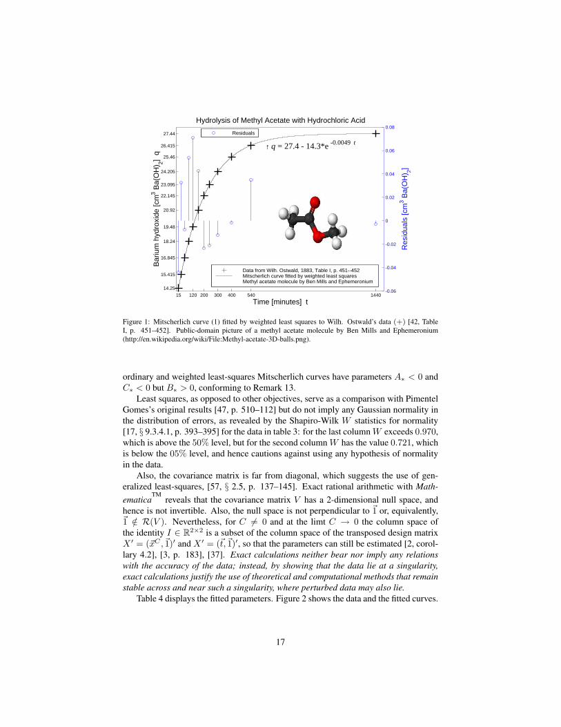
useful in studying greenhouse effects [14]. The significance of the present theory isthat for such data there exists a priori a best-fitting Mitscherlich curve with parametersA∗ < 0 and C∗ < 0 but B∗ > 0, reflecting the postulated type of the reaction.

Example 14. Table 1, in its first three columns, shows Ostwald’s data on the hydrol-ysis of methyl acetate (M = CH3COOCH3) with hydrochloric acid (A = HCl) intomethanol (N = CH3OH) and acetic acid (C = CH3COOH), according to the stoichio-metric equation

A + M + H2O A + N + C.

Thus in dilute solutions with initial concentrations b := [M]0 > 0 and [C]0 = 0 = [N]0at time t = 0, the sums of concentrations remain constant: [C] + [M] = [M]0 =[N] + [M] at all times. At any time, the concentration (x) of acetic acid [C] can bemeasured by titration with a volume (y) of barium hydroxide (Ba(OH)2) [42], whichprovides a means to test models of the mechanism of the reaction: in chemistry, the typeof the fitted curve, rather than the values of its parameters, is “the principal evidencefor the postulated mechanisms” of a reaction [24, p. 10]. For example, if the speeddx/dt of the reaction is proportional to the product of concentrations a := [A] and[M] = [M]0 − [C] = b− x, then

dx

dt= kf · a · (b− x), (48)

where kf > 0 is the forward constant of proportionality. For x(0) = 0, the solutionis x(t) = b · (1 − e−kf ·a·t). However, the initial conditions may not be ideal [42], sothat if t0 denotes the time when conditions begin to be ideal, then x(t0) need not be0. Moreover, the measured quantity is not x but the volume y of barium hydroxidethat titrates the concentration of acetic acid, and the solution of hydrochloric acid alonetitrates at 13.33 [cm3] of barium hydroxide [42, p. 452]. Therefore, y(t) = B+A ·eC·twith y(0) = B + A · eC·0 = B + A ≈ 13.33 after re-setting the clock to 0 at t0.Also, limt→∞ y(t) = B with C < 0. Thus A and B reflect the initial and finalboundary conditions. It is the rate C, with its dependence on such factors as pressureand temperature, that reflects the physical mechanisms of the reaction [14], [19].

Table 1 also shows the mean yk Ostwald’s two measurements yk,1 and yk,2 at eachtime tk. Calculations confirm that all triples of data are positive, increasing, and log-arithmically concave (sub-exponential), and hence also concave (sub-linear). Con-sequently, ordinary and weighted least-squares Mitscherlich curves have parametersA∗ < 0 and C∗ < 0 but B∗ > 0, conforming to Remark 13. The last column inTable 1 shows the reciprocals of the variances of yk,1 and yk,2 at each time tk, normal-ized to add to 1, which can be used as weights. Table 2 shows the fitted weighted andunweighted Mitscherlich parameters.

According to Ostwald the half-life is about 140 [s] [42, p. 453], which correspondsto C = ln(2)/140 ≈ 0.00495, agreeing to two significant digits with the fitted values.

Remark 15. Although the literature on this topic focuses on ordinary least squares,each measurement may involve a procedure that requires a substantial amount of time,

15

Table 1: Titration of hydrochloric acid and methyl acetate with barium hydroxide [42, Table I, p. 451–452].TIME BARIUM HYDROXIDE

[MIN] [cm3] [cm3] MEAN∗ SQUARED WEIGHTS †

15 14.22 14.28 14.250 0.01088635 15.34 15.49 15.465 0.00174260 16.84 16.85 16.845 0.39189590 18.23 18.25 18.240 0.097974

120 19.51 19.45 19.480 0.010886160 20.90 20.94 20.920 0.024493200 22.19 22.10 22.145 0.004838240 23.14 23.05 23.095 0.004838300 24.20 24.21 24.205 0.391895400 25.42 25.50 25.460 0.006123540 26.40 26.43 26.415 0.043544

1440 27.47 27.41 27.440 0.010886

∗Re-computed from the previous two columns, as opposed to Ostwald’s rounded mean.†Normed reciprocals of the variances computed from the preceding three columns, rounded for display

purposes.

Table 2: Fitting a Mitscherlich curve (1) to the data (+) in Table 1 and Figure 1 with Matlab 7 on Mac Pro.REGRESSION FITTED VALUES FIT

A B C A+ B R2 = 1− F (C)〈q,q〉

F (C)

〈~1,~1〉Ostwald [42] −0.00495 13.33Unweighted −14.264 27.45 −0.00490 13.190 0.999937 0.00111Weighted −14.268 27.46 −0.00492 13.191 0.999961 0.00054

so that the uncertainty in the “independent” variable may be comparable to the uncer-tainty in the “dependent” variable (John E. Douglas: [19] and personal communica-tion).

6.2. Mitscherlich Curves Fitted by Generalized Least SquaresThis subsection shows Mitscherlich curves fitted to correlated data by ordinary,

weighted, and generalized least squares. In the range of fertilizer levels where cropyield increases with fertilizer use, Mitscherlich curves fit the data better than othercurves do, and their parameters have biological interpretation: B is the asymptoticleast upper bound on yield, C is the increase in yield per additional unit of fertilizer,and A corresponds to the yield without any fertilizer [7, Ch. 1].

Example 16. F. Pimentel Gomes fitted Mitscherlich’s curves to the data in Table 3[47, p. 510]. The sums of squares, weights, and Shapiro-Wilk’s W were computedseparately.

With yk denoting the mean of the four yields at each concentration tk of fertilizer,calculations confirm that all triples of data are positive, increasing, and logarithmi-cally concave (sub-exponential), and hence also concave (sub-linear). Consequently,

16

15 120 200 300 400 540 1440

14.25

15.415

16.845

18.24

19.48

20.92

22.145

23.095

24.205

25.46

26.415

27.44

Time [minutes] t

Bar

ium

hyd

roxi

de [c

m3 B

a(O

H) 2]

q q = 27.4 - 14.3*e -0.0049 t↑

Hydrolysis of Methyl Acetate with Hydrochloric Acid

Data from Wilh. Ostwald, 1883, Table I, p. 451--452Mitscherlich curve fitted by weighted least squaresMethyl acetate molecule by Ben Mills and Ephemeronium

-0.06

-0.04

-0.02

0

0.02

0.04

0.06

0.08

Res

idua

ls [c

m3 B

a(O

H) 2]

Residuals

Figure 1: Mitscherlich curve (1) fitted by weighted least squares to Wilh. Ostwald’s data (+) [42, TableI, p. 451–452]. Public-domain picture of a methyl acetate molecule by Ben Mills and Ephemeronium(http://en.wikipedia.org/wiki/File:Methyl-acetate-3D-balls.png).

ordinary and weighted least-squares Mitscherlich curves have parameters A∗ < 0 andC∗ < 0 but B∗ > 0, conforming to Remark 13.

Least squares, as opposed to other objectives, serve as a comparison with PimentelGomes’s original results [47, p. 510–112] but do not imply any Gaussian normality inthe distribution of errors, as revealed by the Shapiro-Wilk W statistics for normality[17, § 9.3.4.1, p. 393–395] for the data in table 3: for the last columnW exceeds 0.970,which is above the 50% level, but for the second column W has the value 0.721, whichis below the 05% level, and hence cautions against using any hypothesis of normalityin the data.

Also, the covariance matrix is far from diagonal, which suggests the use of gen-eralized least-squares, [57, § 2.5, p. 137–145]. Exact rational arithmetic with Math-ematica

TMreveals that the covariance matrix V has a 2-dimensional null space, and

hence is not invertible. Also, the null space is not perpendicular to ~1 or, equivalently,~1 /∈ R(V ). Nevertheless, for C 6= 0 and at the limt C → 0 the column space ofthe identity I ∈ R2×2 is a subset of the column space of the transposed design matrixX ′ = (~xC ,~1)′ and X ′ = (~t,~1)′, so that the parameters can still be estimated [2, corol-lary 4.2], [3, p. 183], [37]. Exact calculations neither bear nor imply any relationswith the accuracy of the data; instead, by showing that the data lie at a singularity,exact calculations justify the use of theoretical and computational methods that remainstable across and near such a singularity, where perturbed data may also lie.

Table 4 displays the fitted parameters. Figure 2 shows the data and the fitted curves.

17

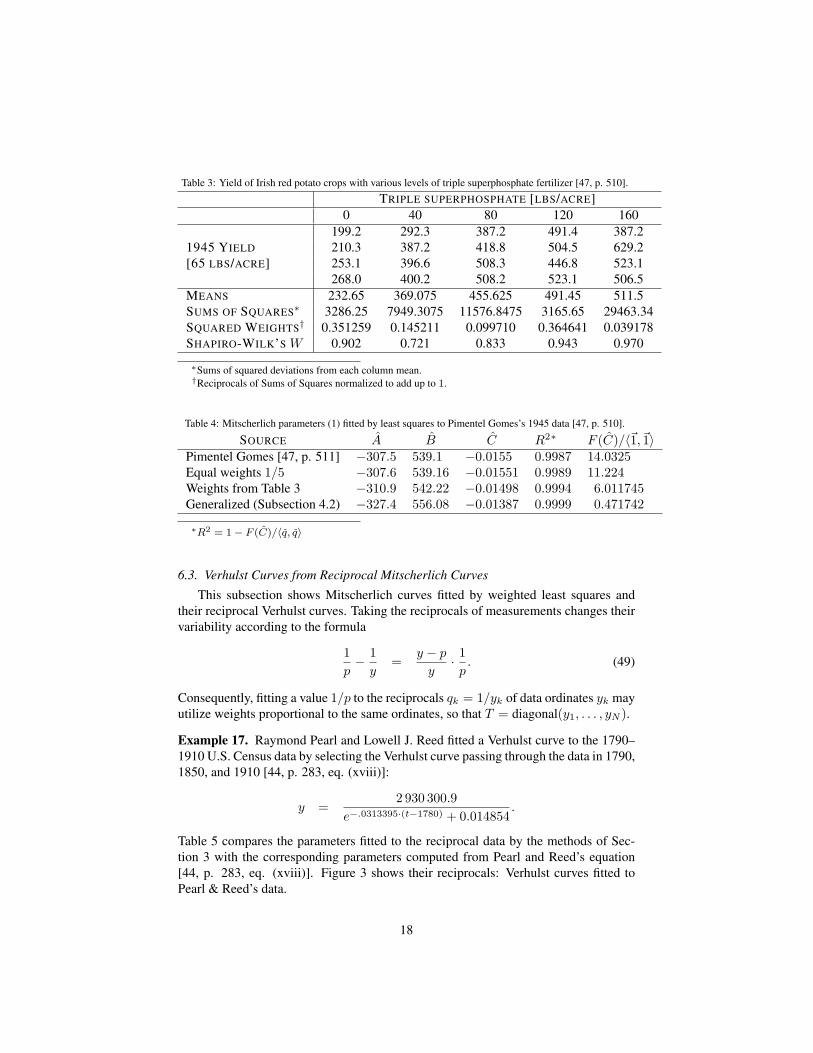
Table 3: Yield of Irish red potato crops with various levels of triple superphosphate fertilizer [47, p. 510].

TRIPLE SUPERPHOSPHATE [LBS/ACRE]0 40 80 120 160

199.2 292.3 387.2 491.4 387.21945 YIELD 210.3 387.2 418.8 504.5 629.2[65 LBS/ACRE] 253.1 396.6 508.3 446.8 523.1

268.0 400.2 508.2 523.1 506.5MEANS 232.65 369.075 455.625 491.45 511.5SUMS OF SQUARES∗ 3286.25 7949.3075 11576.8475 3165.65 29463.34SQUARED WEIGHTS† 0.351259 0.145211 0.099710 0.364641 0.039178SHAPIRO-WILK’S W 0.902 0.721 0.833 0.943 0.970

∗Sums of squared deviations from each column mean.†Reciprocals of Sums of Squares normalized to add up to 1.

Table 4: Mitscherlich parameters (1) fitted by least squares to Pimentel Gomes’s 1945 data [47, p. 510].

SOURCE A B C R2∗ F (C)/〈~1,~1〉Pimentel Gomes [47, p. 511] −307.5 539.1 −0.0155 0.9987 14.0325Equal weights 1/5 −307.6 539.16 −0.01551 0.9989 11.224Weights from Table 3 −310.9 542.22 −0.01498 0.9994 6.011745Generalized (Subsection 4.2) −327.4 556.08 −0.01387 0.9999 0.471742

∗R2 = 1− F (C)/〈q, q〉

6.3. Verhulst Curves from Reciprocal Mitscherlich Curves

This subsection shows Mitscherlich curves fitted by weighted least squares andtheir reciprocal Verhulst curves. Taking the reciprocals of measurements changes theirvariability according to the formula

1p− 1y

=y − py· 1p. (49)

Consequently, fitting a value 1/p to the reciprocals qk = 1/yk of data ordinates yk mayutilize weights proportional to the same ordinates, so that T = diagonal(y1, . . . , yN ).

Example 17. Raymond Pearl and Lowell J. Reed fitted a Verhulst curve to the 1790–1910 U.S. Census data by selecting the Verhulst curve passing through the data in 1790,1850, and 1910 [44, p. 283, eq. (xviii)]:

y =2 930 300.9

e−.0313395·(t−1780) + 0.014854.

Table 5 compares the parameters fitted to the reciprocal data by the methods of Sec-tion 3 with the corresponding parameters computed from Pearl and Reed’s equation[44, p. 283, eq. (xviii)]. Figure 3 shows their reciprocals: Verhulst curves fitted toPearl & Reed’s data.

18

0 40 80 120 160

232.65

369.075

455.625

491.45

511.5

Triple superphosphate 3 Ca(H2 O

4 P)

2 [lbs/acre] t

1945

Mea

n Ir

ish

pota

to y

ield

[65

lbs/

acre

] q

q = 543. - 311.*e -0.01497 t↑

q = 539. - 308.*e -0.01551 t →

q = 556. - 327.*e -0.01387 t →

1945 Mean Irish Potatoes vs. Triple Superphosphate Fertilizer

1945 means of data from Pimentel Gomes, Biometrics, 1953Mitscherlich curve fitted by unweighted least squaresMitscherlich curve fitted by weighted least squaresMitscherlich curve fitted by generalized least squaresPhotograph Idaho Potato Commission

Figure 2: Mitscherlich’s shifted exponential (1) fitted to F. Pimentel Gomes’s 1945 data (+) [47, p. 510] byweighted (−−) unweighted (· · · ) and generalized (−) least squares.

1790 1810 1830 1850 1870 1890 1910

0.3929

0.9638

1.7069

2.3192

3.1443

3.8558

5.0156

6.2948

7.5995

9.1972

x 107

time [years] t

U.S

. pop

ulat

ion

[per

sons

] y

U.S. Population (Homo sapiens)

y = 197417484./(1+e60.04-0.0314t ) →

y = 2930301./[0.0149+e-0.0313(t-1780) ] →

Data from Pearl & ReedReciprocal Mitscherlich curveVerhulst curve by Pearl & ReedEarth lights by NASA

-1.5

-1

-0.5

0

0.5

1

x 106

Res

idua

ls [p

erso

ns]

Residuals, L. S.

Residuals, P & R

Figure 3: Verhulst curve (6) fitted to the reciprocals of Pearl & Reed’s data (+) [44,p. 277, Table 1] as the reciprocal of the fitted Mitscherlich curve. Image courtesy NASA(http://eoimages.gsfc.nasa.gov/ve/1438/earth lights lrg.jpg).

Remark 18. Bradley [8] argues by dimensional analysis that the ratio R := (K −y)/y = (q − B)/B = q/B − 1 is a quantity more natural than y. Still, large positivevalues of y have small positive reciprocals q, with yet smaller differences of positive re-ciprocals, so that fitting curves to reciprocal data amounts to assigning smaller weightsto larger data.

6.4. West Growth Curves Fitted by Non-Linear Least-SquaresThe present section demonstrates how to use the foregoing theory to fit West’s

ontogenetic growth curves to data on the growth of individual organisms from a speciesapparently not yet fitted in this way.

19

Table 5: Fitting a Mitscherlich curve (1) and Verhulst curve (6) to the data (+) in Figure 3 with Matlab 7 ona Mac Pro.

REGRESSION FITTED VALUES FIT ∗

K D C R2† F (C)/〈~1,~1〉Weighted least-squares 197 417 484 60.039 −0.03136 0.99951 10−19

[44, p. 283, eq. (xviii)] 197 254 931 59.994 −0.03134 0.99947 10−19

∗Relative to the Mitscherlich curve fitted to the weighted reciprocals of the data.†1− F (C)/〈q, q〉

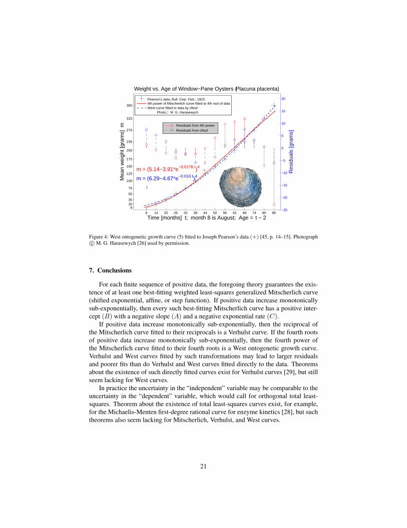
Example 19. Joseph Pearson measured the weight of Placuna placenta (window-paneoysters) semi-yearly [45, p. 14–15]. He does not state the birth date of Oysters, buthis graphically fitted growth curve (shown without any formula [45, Fig. 2, p. 18])passes through (February, 0) [month, mm]. Other sources confirm that in that part ofthe world oysters spawn in February–April and October–December [38]. To avoid anyguesswork the present example fits West’s ontogenetic curves to Pearson’s listed timesinstead of estimated ages. However, the uncertainty in age may be comparable to theuncertainty in weight.

Figure 4 shows that Pearson’s data increase monotonically. Theorem 7 then guar-antees the existence of a least-squares Mitscherlich curves for the fourth roots of thedata, with the same sign for A and C. Table 6 lists the computed Mitscherlich parame-ters A, B, and C. Table 7 gives the West parameters a, m0, and M computed from A,B, and C. Table 7 also provides the West parameters fitted directly to Pearson’s data(as indicated by West et. al [62, p. 628, after eq. (5)]), here by MATLAB’s cftool.Figure 4 shows that West’s direct method yields smaller residuals than does the fourthpower of the fitted Mitscherlich curve. Still, no theorems guaranteeing the existence ofsuch a best-fitting West curve seem known.

Table 6: Fitting a Mitscherlich curve (1) to the fourth root of the data (+) in Figure 4 with Matlab 7 on aMac Pro.

REGRESSION FITTED VALUES FIT∗

A B C R2 = 1− F (C)〈q,q〉

F (C)

〈~1,~1〉Unweighted −3.9064 5.1422 −0.017628 0.9972 0.002

∗Relative to the Mitscherlich curve fitted to the transformed data (t,m1/4).

Table 7: West ontogenetic growth curves (5) fitted to the data (+) in Figure 4, with Matlab 7 on a Mac Pro.

FROM a [g1/4/month] m0 [g] M [g] S∗

Table 6. 0.3626 2.3323 699.2 −1.01MATLAB’s cftool 0.2549 6.937 1565 −1.04

∗Slope of the total least-squares line fitted to Rk = ln[1− (mk/M)1/4] vs. τk = tk · a/(4 ·M1/4).

20

8 14 20 26 32 38 44 50 56 62 68 74 80 86

82035

55

75

100

125

150

175

205

235

275

315

360

Time [months] t; month 8 is August; Age = t − 2

Mea

n w

eigh

t [gr

ams]

m

Weight vs. Age of Window−Pane Oysters (Placuna placenta)

m = (5.14−3.91*e−0.0176 t)4 →

m = (6.29−4.67*e−0.010 t)4

↓

Pearson′s data, Bull. Ceyl. Fish., 19234th power of Mitscherlich curve fitted to 4th root of dataWest curve fitted to data by cftool Photo M. G. Harasewych

−25

−20

−15

−10

−5

0

5

10

15

20

Res

idua

ls [g

ram

s]

Residuals from 4th power

Residuals from cftool

Figure 4: West ontogenetic growth curve (5) fitted to Joseph Pearson’s data (+) [45, p. 14–15]. Photographc©M. G. Harasewych [26] used by permission.

7. Conclusions

For each finite sequence of positive data, the foregoing theory guarantees the exis-tence of at least one best-fitting weighted least-squares generalized Mitscherlich curve(shifted exponential, affine, or step function). If positive data increase monotonicallysub-exponentially, then every such best-fitting Mitscherlich curve has a positive inter-cept (B) with a negative slope (A) and a negative exponential rate (C).

If positive data increase monotonically sub-exponentially, then the reciprocal ofthe Mitscherlich curve fitted to their reciprocals is a Verhulst curve. If the fourth rootsof positive data increase monotonically sub-exponentially, then the fourth power ofthe Mitscherlich curve fitted to their fourth roots is a West ontogenetic growth curve.Verhulst and West curves fitted by such transformations may lead to larger residualsand poorer fits than do Verhulst and West curves fitted directly to the data. Theoremsabout the existence of such directly fitted curves exist for Verhulst curves [29], but stillseem lacking for West curves.

In practice the uncertainty in the “independent” variable may be comparable to theuncertainty in the “dependent” variable, which would call for orthogonal total least-squares. Theorem about the existence of total least-squares curves exist, for example,for the Michaelis-Menten first-degree rational curve for enzyme kinetics [28], but suchtheorems also seem lacking for Mitscherlich, Verhulst, and West curves.

21

8. Acknowledgments

This work was supported in part by a Faculty Research and Creative Works Grantfrom Eastern Washington University. I thank John E. Douglas, retired professor ofchemistry, for his expert advice on the case studies. I also thank an anonymous refereefor pointing out very relevant references to the literature.

References

[1] A.C. Aitken, On least squares and linear combinations of observations, Proceed-ings of the Royal Society of Edinburgh, Section A 55 (1935) 42–47.

[2] I.S. Alalouf, Oan explicit treatment of the general linear model with singularcovariance matrix, Sankhya: The Indian Journal of Statistics 40 (1978) 65–73.

[3] A. Albert, The Gauss-Markov theorem for regression models with possibly sin-gular covariances, SIAM Journal on Applied Mathematics 24 (1973) 182–187.

[4] L.J.S. Allen, An Introduction to Mathematical Biology, Pearson/Prentice Hall,Upper Saddle River, NJ, 2007. ISBN 0-13-035216-0; QH323.5.A436 2007;LCCC No. 2006042585; 570.1’5118–dc22.

[5] G.L. Ashline, J.A. Ellis-Monaghan, Microcosm macrocosm: Population modelsin biology and demography, in: P.J. Campbell (Ed.), UMAP Modules: Tools forTeaching 1999, COMAP, Arlington, MA, 2000, pp. 39–80. Reprinted as Module777, COMAP, Bedford, MA, 1999.

[6] A. Bjorck, Numerical Methods for Least Squares Problems, Society for Indus-trial and Applied Mathematics, Philadelphia, PA, 1996. ISBN 0-89871-360-9;QA214.B56 1996; LCCC No. 96-3908; 512.9’42–dc20.

[7] C.A. Black, Soil Fertility Evaluation and Control, Lewis Publishers, Boca Raton,FL, 1993. ISBN 0-87371-834-8; S596.7.B545 1992; 631.4’22–dc20; LCCC No.92-25089.

[8] D. Bradley, Verhulst’s logistic curve, The College Mathematics Journal 32 (2001)94–98.

[9] J. Bukac, Polynomials associated with exponential regression, ApplicationesMathematicae (Warsaw) 28 (2001) 247–255.

[10] J. Bukac, Nonexistence in reciprocal and logarithmic regression, Analysis in The-ory and Applications 19 (2003) 255–265.

[11] J. Bukac, Nonexistence in power and gamma density regression, sum of nonneg-ative terms, Analysis in Theory and Applications 21 (2005) 38–52.

[12] A. Buse, Goodness of fit in generalized least squares estimation, The AmericanStatistician, 27 (1973) 106–108.

22

[13] F. Cavallini, Fitting a logistic curve to data, College Mathematics Journal 24(1993) 247–253.

[14] G. Chen, J. Laane, S.E. Wheeler, Z. Zhang, Greenhouse gas molecules: A math-ematical perspective, Notices of the American Mathematical Society 58 (2011)1421–1434.

[15] W.M. Chow, Parameter estimation for simple nonlinear models, Communicationsof the ACM 2 (1959) 28–29.

[16] H. Cramer, Mathematical Methods of Statistics, Princeton Landmarks in Mathe-matics, Princeton University Press, Princeton, NJ, 1999. ISBN 0-691-000547-8;QA276.C72 1999; 99-12156; 519.5–dc21; first edition: Almqvist & Wiksells,Uppsala, Sweden, 1945.

[17] R.B. D’Agostino, Tests for the normal distribution, in: R.B. D’Agostino, M.A.Stephens (Eds.), Goodness-of-Fit Techniques, volume 68 of Statistics: Textbooksand Monographs, Marcel Dekker, New York, NY, 1986, pp. 367–419. ISBN 0-8247-7487-6; QA277.G645 1986; 519.5’6; LCCC No. 86-4571.

[18] J.E. Dennis, Jr., R.B. Schnabel, Numerical Methods for Unconstrained Optimiza-tion and Nonlinear Equations, volume 16 of Classics In Applied Mathematics,Society for Industrial and Applied Mathematics, Philadelphia, PA, 1996. ISBN0-89871-364-1; QA402.5.D44 1996; 95–51776.

[19] J.E. Douglas, B.S. Rabinovitch, F.S. Looney, Kinetics of the thermal cis-transisomerization of dideuteroethylene, Journal of Chemical Physics 23 (1955) 315–323.

[20] N.R. Draper, H. Smith, Applied Regression Analysis, Wiley, New York, NY,1966. QA276.D68; 66-17641.

[21] F. Dubeau, Y. Mir, Existence of optimal weighted least squares estimate for three-parametric exponential model, Comm. Statist. Theory Methods 37 (2008) 1383–1398.

[22] M.L. Eaton, Multivariate statistics, Wiley Series in Probability and MathematicalStatistics: Probability and Mathematical Statistics, John Wiley & Sons Inc., NewYork, 1983. A vector space approach.

[23] V. Elangovan, H. Raghuram, E.Y.S. Priya, G. Marimuthu, Wing morphology andflight performance in Rousettus leschenaulti, Journal of Mammalogy 85 (2004)806–812.

[24] A.A. Frost, R.G. Pearson, Kinetics and Mechanism: A Study of HomogeneousChemical Reactions, Wiley, New York, NY, second edition, 1961. LCCC No.61-6773.

[25] G.F. Gause, The Struggle for Existence, Dover, Mineola, NY, 2003. QH375.G352003; 576.8’2–dc21; LCCC No 2002037091. First published by Hafner in 1969.

23

[26] M.G. Harasewych, F. Moretzsohn, The Book of Shells: A Life-Size Guide toIdentifying and Classifying Six Hundred Seashells, University of Chicago Press,Chicago and London, 2010. ISBN 0226315770.

[27] R.V. Hogg, A.T. Craig, Introduction to Mathematical Statistics, Macmillan, NewYork, NY, fourth edition, 1978. ISBN 0-02-355710-9; QA276.H59 1978; 77-2884; 519.

[28] D. Jukic, K. Sabo, R. Scitovski, Total least squares fitting Michaelis-Menten en-zyme kinetic model function, J. Comput. Appl. Math. 201 (2007) 230–246.

[29] D. Jukic, R. Scitovski, Solution of the least-squares problem for logistic function,J. Comput. Appl. Math. 156 (2003) 159–177.

[30] H.P. Kuang, Forecasting future enrollment by curve-fitting techniques, The Jour-nal of Experimental Education 23 (1955) 271–274.

[31] M. Kunitz, J.H. Northrop, Isolation from beef pancreas of crystalline trypsinogen,trypsin, a trypsin inhibitor, and an inhibitor-trypsin compound, Journal of GeneralPhysiology 19 (1936) 901–1007.

[32] C.L. Lawson, R.J. Hanson, Solving Least Squares Problems, volume 15 of Clas-sics In Applied Mathematics, Society for Industrial and Applied Mathematics,Philadelphia, PA, 1995. 0-89871-356-0; QA275.L38 1995; 95-35178; 511’.42–dc20.

[33] D. Leach., Re-evaluation of the logistic growth curve for human populations,Journal of the Royal Statistical Society. Series A. General 144 (1981) 94–103.

[34] D. Leech, K. Cowling, Generalized regression estimation from grouped observa-tions: A generalization and an application to the relationship between diet andmortality, Journal of the Royal Statistical Society 145 (1982) 208–223.

[35] T.R. Malthus, An Essay on the Principle of Population, as it affectsthe Future Improvement of Society, etc., J. Johnson, London, UK, 1798.http://www.econlib.org/library/Malthus/malPop.html.

[36] M.R. McDonald, M. Kunitz, The effect of calcium and other ions on the autocat-alytic formation of trypsin from trypsinogen, Journal of General Physiology 25(1941) 53–73.

[37] T.D. Morley, A Gauss-Markov theorem for infinite dimensional regression mod-els with possibly singular covariance, SIAM Journal on Applied Mathematics 37(1979) 257–260.

[38] K.A. Narasimham, Biology of windowpane oyster Placenta placenta (lin-naeus) in Kakinada Bay, Indian Journal of Fisheries 31 (1984) 272–284. ISSN:05372003.

[39] Y. Nievergelt, Increasing data with a negative slope, The American Statistician 65(2011).

24

[40] Y. Nievergelt, Real and generic data without unconstrained best-fitting Verhulstcurves and sufficient conditions for median Mitscherlich and Verhulst curves toexist, The American Mathematical Monthly 119 (2012) 211–234.

[41] W. Ostwald, Studien zur chemischen Dynamik. Erste Abhandlung: Die Ein-wirkung der Sauren auf Acetamid, Journal fur Praktische Chemie 27 (1883) 1–39.

[42] W. Ostwald, Studien zur chemischen Dynamik. Zweite Abhandlung: Die Ein-wirkung der Sauren auf Methylacetat, Journal fur Praktische Chemie 28 (1883)449–495.

[43] H.D. Patterson, A simple method for fitting an asymptotic regression curve, Bio-metrics 12 (1956) 323–329.

[44] R. Pearl, L.J. Reed, On the rate of growth of the population of the United Statessince 1790 and its mathematical representation, Proceedings of the NationalAcademy of Sciences 6 (1920) 199–272.

[45] J. Pearson, Statistics dealing with the growth-rate, &c., of Placuna placenta, Bul-letin of the Ceylon Fisheries I (1923) 13–64.

[46] J.F. Pechere, H. Neurath, Studies on the autocatalytic activation of trypsinogen,Journal of Biological Chemistry 229 (1957) 389–407.

[47] F. Pimentel Gomes, The use of Mitscherlich’s regression law in the analysis ofexperiments with fertilizers, Biometrics 9 (1953) 498–516.

[48] R.L. Plackett, Principles of Regression Analysis, Oxford University Press, Lon-don, UK, 1960. QA276.P5.

[49] L.J. Reed, J. Berkson, The application of the logistic function to experimentaldata, The Journal of Physical Chemistry 33 (1929) 760–779.

[50] R.E. Ricklefs, A graphical method of fitting equations to growth curves, Ecology48 (1967) 978–983.

[51] P.D. Ritger, N.J. Rose, Differential Equations with Applications, Dover, NewYork, NY, 2000. ISBN: 0-486-41154-0; ISBN 13: 9780486411545; QA371.R442000; 515’.35—dc21; LCCC No. 00-026399. First edition by McGraw-Hill, NewYork, NY, 1968.

[52] B. Schulman, Using original sources to teach the logistic equation, UMAP Jour-nal 18 (1997) 375–402. Reprinted as Module 766, COMAP, Lexington, MA,1997, and in [53]; http://www.comap.com/pdf/425/99766.pdf.

[53] B. Schulman, Using original sources to teach the logistic equation, in: P.J. Camp-bell (Ed.), UMAP Modules: Tools for Teaching 1997, COMAP, Arlington, MA,1998, pp. 163–190. ISBN 0-912843-46-2.

[54] W.L. Stevens, Asymptotic regression, Biometrics 7 (1951) 247–267.

25

[55] G.W. Stewart, Errors in variables for numerical analysts, in: S. Van Huffel(Ed.), Recent Advances in Total Least Squares and Errors-In-Variables Models:Proceedings of the Second International Workshop on Total Least Squares andErrors-in-Variables Modeling, Leuven, Belgium, August 21–24, 1996, Societyfor Industrial and Applied Mathematics, Philadelphia, PA, 1997, pp. 3–10. ISBN0-89871-393-5; 96-72486.

[56] J. Stoer, R. Bulirsch, Introduction to Numerical Analysis, Springer-Verlag, NewYork, NY, third edition, 2002. ISBN 0-387-95452-X; QA297.S8213 2002; 2002-019729; 519.4–dc21.

[57] G. Strang, Introduction to Applied Mathematics, Wellesley-Cambridge Press,Wellesley, MA, 1986. ISBN 0-9614088-0-4; QA37.2.S87 1986; 84-52450; 510.

[58] M.E. Turner, R.J. Monroe, H.L. Lucas, Jr., Generalized asymptotic regression andnon-linear path analysis, Biometrics 17 (1961) 120–143.

[59] P.F. Verhulst, Notice sur la loi que la population suit dans son accroissement,Correspondance Mathematique et Physique 10 (1838) 113–121.

[60] P.F. Verhulst, Recherches mathematiques sur la loi d’accroissement de la popula-tion, Nouveaux Memoires de l’Academie Royale des Sciences et Belles-Lettresde Bruxelles 18 (1845) 1–45.

[61] G. de Vries, T. Hillen, M. Lewis, J. Muller, B. Schonfisch, A Course in Mathe-matical Biology, volume 12 of Mathematical Modeling and Computation, Societyfor Industrial and Applied Mathematics, Philadelphia, PA, 2006. ISBN 0-89871-612-8; QH323.5.C69 2006; 570.1’5118–dc22; LCCC No. 2006044305.

[62] G.B. West, J.H. Brown, B.J. Enquist, A general model for ontogenetic growth,Nature 413 (2001) 628–631.

[63] K. Yosida, Functional Analysis, volume 123 of Die Grundlehren der mathema-tischen Wissenschaften in Enizeldarstellungen, Springer-Verlag, New York, NY,fourth edition, 1974. ISBN 0-387-06812-0; QA320Y6 1974; 74-12123.

[64] G. Zyskind, F.B. Martin, On best linear estimation and a general Gauss-Markovtheorem in linear models with arbitrary nonnegative covariance structure, SIAMJournal on Applied Mathematics 17 (1969) 1190–1202.

26