On the General Motion-Planning Problem with Two Degrees …On the General Motion-Planning Problem...

Discrete Comput Geom 4:491-521 (1989) [)i~'rel~ N Comlmtati'sml

On the General Motion-Planning Problem with Two Degrees of Freedom*

Leonidas J. Guibas , 1"2 Micha Sharir, 3: and Shmuel Sifrony 3

DEC Systems Research Center, 130 Lytton Avenue, Palo Alto, CA 94301, USA

Computer Science Department, Stanford University, Stanford, CA 94305, USA

3 School of Mathematical Sciences, Tel-Aviv University, 69978 Tel Aviv, Israel

4 Courant Institute of Mathematical Sciences, New York University, 251 Mercer Street, New York, NY 10012, USA

Abstract. We show that, under reasonable assumptions, any collision-avoiding motion-planning problem for a moving system with two degrees of freedom can be solved in time O(A~(n) log 2 n), where n is the number of collision constraints imposed on the system, s is a fixed parameter depending, e.g., on the maximum algebraic degree of these constraints, and A~(n) is the (almost linear) maximum length of (n, s) Davenport-Schinzel sequences. This follows from an upper bound of O(A.~(n)) that we establish for the combinatorial complexity of a single connected component of the space of all free placements of the moving system. Although our study is motivated by motion planning, it is actually a study of topological, combinatorial, and algorithmic issues involving a single face in an arrangement of curves. Our results thus extend beyond the area of motion planning, and have applications in many other areas.

I. Introduction

Let B be a robot system having two degrees of freedom (a 2 - D O F system in

short), which is free to move in some two- or three-d imensional space amidst a finite set of m pairwise openly dis joint obstacles O r , . . . , Ore, whose geometry is

* Work on this paper by the second author has been supported by Office of Naval Research Grant N00014-82-K-0381, by National Science Foundation Grant No. NSF-DCR-83-20085, by grants from the Digital Equipment Corporation, and the IBM Corporation. Work by the second and third authors has also been supported by a research grant from the Joint Ramot-lsraeli Ministry of Industry Foundation, and by a research grant from the NCRD--the Israeli National Council for Research and Development.

492 L.J. Guibas, M. Sharir, and S. Sifrony

known to the system. The set of all placements of B is a 2-D parametric space which we denote by AP (the space of "all placements"; intuitively we think of AP as a locally Euclidean manifold which can be covered by a constant and usually small number of patches, each homeomorphic to some simple planar domain). The subset of AP containing all free placements of B (i.e., placements in which B does not intersect U~'=~ O~, and no two subparts of B intersect one another) is referred to as the free configuration space of B, and is denoted by FP (the space of "free placements"); we also denote by BFP the (topological) boundary of FP. The motion-planning problem for B is: given an initial placement Z~ and a (desired) final placement Z2 of B, both belonging to FP, determine whether there exists a collision-free continuous motion of B between these placements, i.e., a continuous path from Zj to Z2 within FP (often we are willing to "compromise" and require only that the path lie in FP u BFP). If so, we also wish to plan such a motion. Since for such a motion to exist, the two given placements must lie in the same connected component of FP (or of FP u BFP), an equivalent formulation of the problem is to calculate a discrete combinatorial representation of the decomposition of FP (or of its closure) into arcwise connected components.

This is a relatively simple instance of the general motion-planning problem; see below for a review of existing work on the problem.

In our case, the boundary BFP of the space FP can in general be defined by a finite number n of collision constraints y ~ , . . . , y~, each of which is the locus of placements of B at which contact is made between a specific subpart of B and a specific subpart of some obstacle or between two specific subparts of B. We assume, as is customary in motion planning, that these constraints are connected and simple algebraic arcs of some small and fixed maximal degree d (but the results obtained in this paper also hold under weaker assumptions--see below).

With no real loss of generality, we assume the space AP of all system placements to be planar. In general, the manifold AP can be more complex. For example, for a planar "Stanford arm," namely a line segment free to slide through a fixed point and also to rotate around it [FWY], AP is cylindrical; for a two-link planar robot arm, AP is toroidal, etc. In these cases we "triangulate" AP, i.e., break it into O(1) planar patches, apply our analysis in each patch separately, and then glue the results together.

Let us form the arrangement A of the arcs y ~ , . . . , y,. This is the planar map whose vertices are the endpoints of these arcs and all their intersection points, whose edges are maximal connected subarcs of the yi's whose interiors do not meet any other arc, and whose faces are the connected components of the complement of U~=~ y~. By Bezout's theorem (see, e.g., p. 54 of [Ha]), the total number o f vertices of A is O(d2n 2) = O(n2); it easily follows from Euler's formula that the number of edges and faces of A is also O(n2).

The above considerations imply that each connected component of FP must be a face o f A. The converse is not true in general, because some faces of A might represent regions of forbidden placements of B. Nevertheless, once A is

On the General Motion-Planning Problem with Two Degrees of Freedom 493

available, we can obtain FP from it in a straightforward way, by pruning away the forbidden faces. In particular, it follows that the combinatorial complexity of FP is O(n2). Calculation of A can be accomplished by a standard line-sweeping technique (as in [BO]), in time O ( ( n + p ) log n), where p is the total number of intersections between the curves yi, and is O(n 2) in the worst-case. An alternative technique has been recently proposed in [EGP*]; it runs in slightly more than quadratic time, and is mentioned below. Other related techniques are given in [CE], [Cl], [Mul] , and [Mu2].

So far we have roughly quadratic-time methods for producing FP. Moreover, these methods are close to optimal in the worst-case, because there are many cases of motion-planning problems with two DOFs in which FP is actually of quadratic size (see below). The key observation of this paper is that in most cases we do not need to calculate the entire FP, but only its connected component C containing the initial given placement Zo of B. Indeed, as long as B moves in a collision-free manner from Zo (and is not artificially "lifted up" and "re-started" in a position lying in a different component of FP), it will have to remain within C. Our goal is thus to precalculate only the component C, rather than the entire FP, and thereby achieve better performance.

Our first main result is that the combinatorial complexity of such a single connected component C is only O(A~+2(n)), where s < - d 2 is the maximum number of intersections of any two constraint curves y , y~. Here A,(n) denotes the maximum length of (n, r) Davenport-Schinzel sequences, i.e., sequences composed of n symbols, which do not contain equal adjacent elements and also do not contain an alternating subsequence of two distinct symbols of length r + 2. It is known [HS], [ASS] that At(n) is almost linear in n for any fixed r. More specifically,

Al(n) = n; Az(n) = 2n - 1 (trivial). A3(n) = O ( n a ( n ) ) , where a(n) is the functional inverse of Ackermann's

function, and thus grows extremely slowly [HS]. A4(n) = O ( n . 2 "(")) [ASS].

A2~(n) = n. 2 °~'~"r-') for s > 2 [ASS]. Azs+l(n) = n. a (n ) °(~'(')'-~) for s >---2 [ASS].

Ats(n) = n. 2 n('~"v-') for s > 2 [ASS].

Our result is actually a general topological property of arrangements of curves. That is, a single face in such an arrangement of n arcs in the plane, any two of which intersect in at most s points, has combinatorial complexity O(A,+2(n)). This result has already been established in [PSS] for the special case of arrangements of line segments, where s = 1 and the complexity of a single face is thus O()L3(n)) = O(na(n) ) . Our result extends a recent (somewhat simpler) result in [SS5], showing that if the yi's are closed Jordan curves, then the complexity of a single face of A is only O(A,(n)) .

Our second main result is an algorithm which, given a collection of n ares ~'1 . . . . ,3,,, and a point Zo not lying on any of them, calculates the face of the arrangement of these arcs that contains Zo. Here we assume that any two ares


7i, Y~ intersect in at most s points, and that any arc 3,, has at most t points of vertical tangency (so that it can be broken up into at most t + 1 x-monotone subarcs); here s and t are assumed to be small fixed constants. Moreover, we assume a model of computation where certain primitive operations involving one or two arcs take constant time; typical such operations are: finding the intersection points of a pair of arcs, finding the points of vertical tangency of a given arc, finding the intersections of an arc with a vertical line, etc. All these assumptions are reasonable if the arcs yi are algebraic of low degree as assumed above. Under these assumptions, our algorithm runs in O(As+2(n) log 2 n) time and O(A,+2(n)) space. Again, in the special case discussed in [PSS] (where the y~'s are line segments arising as the Minkowski difference of the boundaries of two simple polygons), another algorithm, of comparable complexity, has been presented. Recently, Edelsbrunner et al. [EGS] have obtained an O(nct(n) log 2 n) algorithm for calculating a single face in an arbitrary arrangement of line segments. We extend the technique of [EGS] to handle arrangements of curved arcs. The previous algorithm in [PSS] is based on ray shooting in simple polygons (see [CG]). This technique can be applied only in very restricted circumstances (some more of which are mentioned below and discussed in [Sil l in more detail); in particular, it does not seem to generalize to curved arcs. The technique of [EGS] is based on line sweeping, is conceptually simpler, and can be extended to our case, although this generalization requires some additional analysis of the intersection pattern of such arcs, which is developed below.

The special cases (in addition to that in [PSS]) in which the ray-shooting technique can be applied include:

(a)

(b)

Translational motion of a simple polygon P with k sides amidst a collection of n point-obstacles (imagine P translating on a board amidst a collection of pins or pegs tacked to the board). Here we can calculate a connected component of FP in time O(nk~(nk) log nk log n) (which is slightly better than our general bound). The case in which the forbidden subspaces induced by the problem constraints are all polygonal, and their sides have only a fixed and small number k of possible orientations. This would be the case, e.g., for translational motion of a rectilinear simple polygon amidst a collection of rectilinear obstacles. In this case we can calculate a single connected component of FP in time O(nkoe(n) log n), which reduces to O(n log n) in case of rectilinear regions, and which again is better than our general bound.

However, as it turns out, these time bounds can also be obtained by an appropriate fine-tuning of the recursion of the general algorithm given in this paper. For this reason we omit here details concerning this alternative ray-shooting technique.

Some related results for the case of lines or line segments are given in [ EGH 1" ], where, for example, it is shown how to preprocess a collection of n lines in roughly O(n 3/2) randomized expected time and roughly linear space so that the


face in the arrangement of these lines containing any given query point can be retrieved in time roughly O(n~/2+ k), where k is the size of the face.

As mentioned in the Abstract, we regard our topological and algorithmic results as basic important properties of arrangements of curves in the plane. Our results have recently been applied to various other problems. One application in [EGP*] obtains a generalized "horizon theorem" for arrangements of curves, and an incremental algorithm for constructing such arrangements in roughly quadratic time. Another recent application in [AgS] obtains fast algorithms for detecting intersections between two collections of arcs in the plane. Our results have also been recently applied in [SSi] to obtain efficient coordinated motion- planning algorithms for two independent systems with two degrees of freedom each.

Related Work

In an initial series of papers Schwartz and Sharir [SS1]-[SS3], [SA], [SS4] obtained polynomial-time motion-planning algorithms for the general algebraic case and for several specific robot systems. The Schwartz-Sharir algorithms involve decomposition of FP into finitely many simple connected cells and construction of a connectivity graph CG representing adjacency of these cells in FP. Several recent improvements of these initial results have been based on generalized Voronoi diagrams JOY], [OSY1], [OSY2], [LS2], whereas others involve optimized variants of the cell decomposition method [LSI]. Another recent technique, due to Sifrony and Sharir [SIS], obtains a motion-planning algorithm for the special case of a line segment (a "rod") translating and rotating in a 2-D polygonal region by an explicit calculation of :he boundary of FP.

A special case of the 2-DOF motion-planning problem is that of planning a purely translational motion for a planar object B amidst polygonal obstacles. This problem has been studied in [OY] for the case where B is a disk, and in [KS1], [KLPS], [BZ], and [LS2] for the case where B is a convex polygon. These purely translational cases turn out to be more favorable than general 2-DOF problems, in that the FP boundary in each of the above two cases contains only O(n) vertices, and can be optimally calculated in O(n log n) time using generalized Voronoi diagrams (see JOY] and [LS2]). In general, however, the FP boundary for 2-DOF motion-planning problems can contain l)(n 2) vertices (this happens even in the purely translational case when the moving system is a nonconvex polygon; see a remark in [KS1]).

Additional discussion of related results is given in Section 2. The paper is organized as follows. In Section 2 we introduce the terminology

and derive a few initial observations about the problem structure. In Section 3 we analyze the combinatorial complexity of a single component of FP, or, more generally, of a single face in an arrangement of curves. In Section 4 we present an efficient algorithm for calculating a single such face, and in Section 5 we conclude with a discussion of several simple cases, extensions, and open problems.

496 L.J. Guibas, M. Sharir, and S~ Sifrony

2. Terminology and Initial Analysis

We have already described in the Introduction the abstract representation that we use for the general 2-DOF motion-planning problem. In most of what follows, we assume that the space AP of all possible (not necessarily free) configurations of the moving system B can be embedded in the Euclidean plane. The boundary of the free configuration space FP is contained in the union of a collection F of O(n) (algebraic) simple Jordan arcs Yl . . . . . ~/,, where each Yi is the locus of placements Z of B in which a specific subpart of B touches a specific part of some obstacle, or two subparts of B touch one another. Consider the arrangement A = A(F) of the curves 2,~ as defined in the Introduction. Let Zo~ FP be a given initial placement of B. As above, our goal is to calculate the connected component of FP containing Zo, i.e., the face of A containing Zo.

When A P cannot be globally embedded in the plane, e.g., when one degree of freedom 0 is rotational and admits the full 2rr range of orientations, we represent A P as the union of finitely many planar " p a t c h e s ' w i n the above example, these would correspond to the subranges 0 -< 0 -< ~r and 7r - 0 ~ 2 r r - -and apply the foregoing analysis to each of them separately. It is important to note that the number of patches is independent of the geometric complexity of the workspace of the system B, and depends only on the type of degrees of freedom of B.

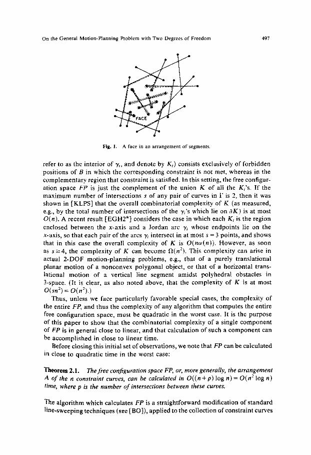
Example. To illustrate these concepts, consider the case of an arbitrary (not necessarily simply connected) k-gon B translating in the plane amidst a collection of polygonal obstacles having a total of m sides. Each placement of B can be specified by the position Z of some fixed reference point inside B. There are n = O(km) constraints defining FP, and they induce n constraint curves, where each such curve yi is the locus of placements of B in which some specific corner of B touches some obstacle edge, or some specific side of B touches some obstacle corner. In this special case it is easily verified that each 3'~ is a line segment, obtained as the Minkowski (vector) difference of the obstacle feature and the feature of B making contact (see, e.g., [KLPS] for more details). Thus in this setting, our problem is to calculate the face in an arrangement of n line segments, which contains a given point Zo (see [EGS] and [EGHI* ] ; a special case of this problem has also been studied in [PSS]). Such a face is illustrated in Fig. 1.

Let F be the collection of the n constraint curves. We assume that these curves are in general position, meaning that no three of them pass through the same point, that no two are tangent to one another, and that no two of them overlap (our analysis can be easily modified to handle degenerate configurations of this kind). As noted, the arrangement A(F) consists of O(n 2) faces, edges, and vertices.

Before plunging into our analysis, let as digress for a moment to consider several special cases of the problem in which the complexity of the entire space FP (not just of a single component of it) is also small. To describe these cases, suppose for a moment that each constraint curve yi is a closed Jordan curve, and that it partitions the plane into two regions, so that one of them (which we


P

Fig. 1. A face in an arrangement of segments.

refer to as the interior of 3',, and denote by Ki) consists exclusively of forbidden positions of B in which the corresponding constraint is not met, whereas in the complementary region that constraint is satisfied. In this setting, the free configuration space FP is just the complement of the union K of all the Ki's. I f the maximum number of intersections s of any pair of curves in F is 2, then it was shown in [KLPS] that the overall combinatorial complexity of K (as measured, e.g., by the total number of intersections of the yi's which lie on a K ) is at most O(n). A recent result [EGH2*] considers the case in which each K~ is the region enclosed between the x-axis and a Jordan arc 3'~ whose endpoints lie on the x-axis, so that each pair of the arcs yi intersect in at most s = 3 points, and shows that in this case the overall complexity of K is O(na(n)) . However, as soon as s__.4, the complexity of K can become f~(n2). This complexity can arise in actual 2-DOF motion-planning problems, e.g., that of a purely translational planar motion of a nonconvex polygonal object, or that of a horizontal translational motion of a vertical line segment amidst polyhedral obstacles in 3-space. (It is clear, as also noted above, that the complexity of K is at most O(sn 2) = O(n2).)

Thus, unless we face particularly favorable special cases, the complexity of the entire FP, and thus the complexity of any algorithm that computes the entire free configuration space, must be quadratic in the worst case. It is the purpose of this paper to show that the combinatorial complexity of a single component of FP is in general close to linear, and that calculation of such a component can be accomplished in close to linear time.

Before closing this initial set of observations, we note that FP can be calculated in close to quadratic time in the worst case:

Theorem 2.1. The free configuration space FP, or, more generally, the arrangement A of the n constraint curves, can be calculated in O ( ( n + p ) log n) = O(n 2 log n) time, where p is the number of intersections between these curves.

The algorithm which calculates FP is a straightforward modification of standard line-sweeping techniques (see [ BO]), applied to the collection of constraint curves


3';. We note that p may be substantially larger than the actual number q of these intersections which lie on OFP. We leave it as an open problem whether FP can be calculated in time O((n + q)log n) (or, in view of the results below, even in time O((n+q) log 2 n)) where q is as above. Another open problem is whether we can apply the topological sweeping technique of lEG] to obtain an algorithm whose complexity does not involve the log n factor.

Remark. A recent result of [EGP*] gives an O(nA~+2(n)) algorithm for calculating the arrangement A(F) using an incremental construction technique, whose analysis is based on the results obtained in this paper. For arrangements of segments, it was shown in [CE] that they can be computed in time O(n log n + t), where t is the number of intersections between the n given segments. Two other papers [CI], [Mul ] give randomized algorithms that construct an arrangement of segments in an incremental fashion; their expected running time is also O(n log n + t). See also [Mu2] for an extension of this technique to the case of arcs.

3. The Complexity of a Single Component of FP

In this section we obtain an almost-linear upper bound on the combinatorial complexity of a single connected component of FP. Specifically, we show:

Theorem 3.1. Under the assumptions made in the preceding section, the combinatorial complexity of any single connected component of FP is at most O(A, +2(n )).

Proof. Let f be the given connected component , and let C be a connected component of its boundary. It suffices to show that if k arcs of F appear along C, then the number of subarcs of these arcs which constitute C is O(A~+2(k)). Thus, without loss of generality, we may assume that all n arcs of F appear along C. For each y; let u;, v~ be its endpoints. Let y~ (resp. yU) be the directed arc 3,, oriented from u; to v; (resp. from vi to ui).

Without loss of generality, assume C is the exterior boundary component of f Traverse C in counterclockwise direction (so that f lies to our left) and let S = (s, , s2, • . . , st) be the circular sequence of oriented curves in F in the order in which they appear along C (if C is unbounded, S is a linear rather than circular sequence). More precisely, if during our traversal of C we encounter a curve y; and follow it in the direction from u~ to v~ (resp. from v; to u~), then we add y+ (resp. Yl) to S. As an example, if the endpoint ui of y~ is on C and is not incident to any other arc, then traversing C past u; will add the pair of elements y~-, y+ to S, and symmetrically for v;. See Fig. 2 for an illustration. Note that in this example both sides of an arc y~ might belong to our connected component ; in our original motion-planning application this usually was not the case, because crossing a constraint curve generally means that the system is passing from free to nonfree placements, but the generalized problem that we study now allows for such two-sidedness.


Fig. 2. Traversing a face boundary and the resulting sequence S.

We use the following notation. We denote the oriented arcs of F as ¢~ . . . . , ¢2,. For each ~:~ we denote by I~:,1 the nonoriented arc yj coinciding with ~. For the purpose of the proof we transform each arc y~ into a very thin closed Jordan curve 3'* by taking two nonintersecting copies of y~ lying very close to one another, and by joining them at their endpoints. This will perturb the component f slightly but, under our assumption on general position, it will not change the combinatorial structure of the boundary of f, and in particular of C. Note that this transformation allows a natural identification of one of the two sides of 3'* with 3'~ and the other side with 3'i-.

We next need the following lemmas:

Lemma 3.2 (The Consistency Lelqma). The portions of each arc ~ appear in S in a circular order which is consistent with their order along the oriented ~ ; that is, there exists a starting point in S (which depends on ~i) such that if we read S in circular order starting from that point, we encounter these portions in their order along ~.

Proof. Let if, -r/ be two portions of ~:~ which appear consecutively along C in this order (i.e., no other portion o f ~ appears along C between ~" and rt). Choose two points x c ~" and y c rt and connect them by the portion a of C traversed from x to y, and by another arc/3 within the interior of 1~:~1". Clearly, a and/3 do not intersect (except at their endpoints) and they are both contained in the complement of (the interior of) f. Thus their union a w/3 is a closed Jordan curve and f is fully contained either in its exterior or in its interior. We claim that any point on ~:~ between l: and r/ is contained in the side of a u/3 which does not contain f. Indeed, connect such a point z to x along an arc p that proceeds very near ~i along the exterior of t~:~t* (see Fig. 3). Clearly, p and/3 are disjoint, and, deforming a slightly as necessary, we can assume that p intersects a transversally and exactly once, which is easily seen to imply our claim. This claim completes the proof of the lemma. []

For each directed arc ~:i consider the linear sequence V~ of all appearances of ~:~ in S, arranged in the order they appear along ~:i. Let /z~ and u~ denote, respectively, the index in S of the first and last elements of V~. Consider S = (s~ . . . . , s,) as a linear, rather than circular, sequence (this step is not needed if


lere

OR

P z

Fig. 3.

i here S C

Illustration of the proof of the consistency lemma.

C is unbounded) . For each arc ~:~, if/~i > vi we split the symbol ~:i into two distinct symbols ~ , , ~:~2, and replace all appearances o f ~:i in S between the places p.~ and t (resp. between 1 and v~) by ~:~ (resp. s¢;2). (Note that Lemma 3.2 implies that we can actually split the arc ~:~ into two connected subarcs, so that all appearances o f ~:~ in S* represent port ions o f the first subarc, whereas all appearances of ~:~2 represent port ions o f the second subarc.) This splitting produces a sequence S*, o f the same length as S, composed of at most 4n symbols.

The assertion o f the theorem is then an immediate consequence o f the following:

Lemma 3.3. S* is a (4n, s + 2 ) Davenport-Schinzel sequence.

Proof. Since it is clear that no two adjacent elements o f S* can be equal, it remains to show that S* does not contain an alternating subsequence o f the form ~'. • • r/. • • ~'. • • r/. • • o f length s + 4. Assume to the contrary that S* does contain such an alternation, and consider any four consecutive elements o f this alternation, which, without loss o f generality, can be assumed to be ~7" • • r/. • • ~7" • • r/. Choose points x, y e ~r and points z, w e r/ so that C passes through these points in the order x, z, y, w. Cons ider the following five Jordan arcs:

flxy = an arc within the interior o f [~J* connect ing x to y; /3~ = an arc within the interior o f ]r/I* connect ing z to w; f l= = the port ion o f C traversed in counterclockwise direction from x to z; /3zy = the port ion o f C traversed in counterclockwise direction from z to y; /3y,~ = the port ion o f C traversed in counterclockwise direction from y to w.

Note that/3=,/3~y,/3~w are pairwise nonintersecting and that they also do not intersect/3xy,/3z~. We claim that fl~y a n d / 3 ~ must intersect one another. Assume


f

iw Byw

Deformed 1o

#xz /~zy #yw ~T ,r y~ q

\ I // \ / k /

Bxy /gzw

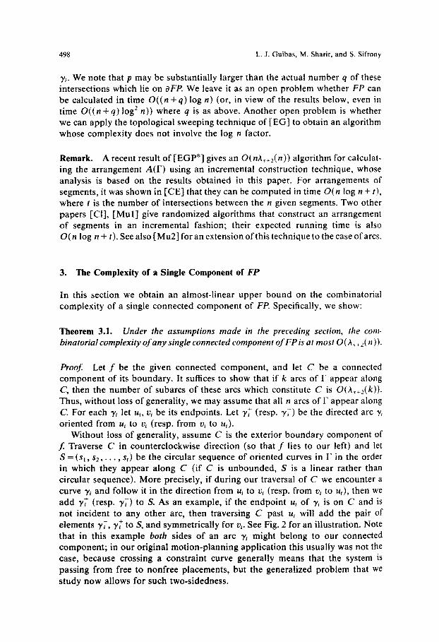
Fig. 4. Illustration of the proof of Lemma 3.3,

the contrary, and consider the planar graph G composed of these five arcs as edges. Clearly, G has three faces, and its edges all lie in the complement of the interior of f. Thus f is fully contained in just one of these faces. Moreover, as /3 = fl~z w/3...,, w flyw is traced from x to w, all points lying on the left side o f /3 sufficiently near it belong to f. By deforming the plane we may assume that lies on the x-axis, with x, z, y, w appearing along it from left to right in this order, that the portion of the upper halfplane sufficiently near ~ is contained in ~ that the two arcs/Jx,, and/3~, emanate downward from the respective points y and z, and that the portions of these arcs within sufficiently small neighborhoods of these two respective points are just straight vertical segments; see Fig. 4.

Let a and b be two points in the relative interior of/3~,/3~.~, respectively, let a', b' be two corresponding points lying below and very close to a, b, respectively. By the properties of G, neither a' nor b' lies in the face of G containing f Moreover, if a' and b' are chosen sufficiently near /3, the straight segment connecting a' to b' will intersect each of/jxy,/jzw in exactly one point. This easily implies that a ' and b' both lie in the same face ~ of G. Consider the closed Jordan curve t3" traced as we move from a to a' along a short segment, from a' to b' along a path that connects these points in ~, from b' to b along another short segment, and finally from b to a along/3. It is easily checked that points along /3~w slightly after z lie on one side of /3* and points on that curve just before w lie on the other side of/3*. Thus/3~w has to intersect/3", which however is impossible because /3* is contained within ~ w/~, which is openly disjoint from/3~,.

This shows that each quadruple of consecutive elements in our alternation induces at least one intersection point between the corresponding arcs /3~y c ~" and/jzw c r/. Moreover, it is easily checked that for any pair of distinct quadruples of this type, either the two corresponding subarcs of the form/3~y along ~ are


disjoint, or the two subarcs fl~w along -q are disjoint. Thus all these intersections must be distinct. Since the number of such quadruples is s + 4 - 3 = s + 1, we obtain a contradict ion, which completes the p roof of the lemma, and thus also o f the theorem. []

Remark. It has been proved recently in [SS5] that if the curves y, in F are closed Jordan curves, or Jordan arcs unbounded in both directions, then the complexity o f a single componen t o f A(F) is at most O(A~(n)).

Remark. Applying our theorem to the case where each % is a line segment, we obtain an upper bound of O ( A 3 ( n ) ) = O(nc~(n)) on the complexity of a single componen t of A(F). The results o f [WS] and [Sh] imply that this bound is tight in the worst case. This special case of the theorem has already been established in [PSS].

4. Calculating a Single Component in an Arrangement of Curves

In this section we show how to calculate a single componen t f in an arrangement o f a collection F o f n Jordan arcs ~/1,. • -, ~/,, having the property that no pair o f them intersect in more than s points. Our algorithm runs in time O(As+2(n) log 2 n) and is thus close to linear. We assume a model o f computat ion involving infinite-precision real arithmetic, in which s tandard operat ions involving one or two curves in F are assumed to take constant time. Moreover, since our technique is based on line sweeping, we assume that the shape o f each curve in F is relatively simple and not too "wiggly." Specifically, we assume that each curve in F has at most t points o f vertical tangency, for some fixed constant t, so that we can break it into at most t + 1 Jordan arcs that are mono tone in the x-direction. Thus, in the remainder of this section we assume each y ~ F to be x -mono tone (this addit ional condit ion is satisfied in most applications; in particular, it holds for curves that are algebraic o f a fixed maximal degree). Also, we assume that the curves o f F are in general position, so that each intersection o f a pair o f these curves is either at a c o m m o n endpoint or is a transversal intersection at a point in the relative interior o f both. We also assume that no two intersection points or endpoints lie on the same vertical line, so as to simplify the description o f our line-sweep algorithm (none o f these assumptions are essential, and simple modifications of our algorithm will make it work also in the presence o f degeneracies). Typical operat ions that are assumed to take constant time are: (a) find the intersection points between a pair of curves in F; (b) find the intersection between a vertical line and a curve in F.

The algorithm that we seek thus receives as input a collection F of n Jordan arcs (or closed curves) with the above properties, and a point x not lying on any o f these curves. Its output is a discrete representat ion of the connected component f o f the ar rangement A(F) containing x. The representat ion that we use is the collection o f the connected components o f the boundary o f f, each given as a circular list o f subarcs and vertices appear ing along that boundary component


in counterclockwise order. The algorithm extends the technique in [EGS] for the calculation of a component (actually of many components simultaneously) in an arrangement of line segments.

The high-level description of our algorithm is quite simple. We use the following divide-and-conquer technique. We split F into two subcollections F, , F2 of roughly n/2 curves each, calculate recursively the components f~,f2 of A(F~), A(F2), respectively, that contain x, and then "merge" these two components to obtain the desired component f. Note t h a t f is the connected component of f~ c~f2 containing x. However, it is generally too expensive to calculate this intersection in its entirety, and then select the component containing x, because the boundaries of f~ and f2 might intersect in many (quadratically many in the worst case) points that do not belong to the boundary of f , and we cannot afford to find all of them.

The set-up for the merge step is as follows. We are given two connected (but not necessarily simply connected) regions in the plane, which we denote respectively as the red region R and the blue region B. Both regions contain the point x in their interior, and our task is to calculate the connected component f of R c~ B which contains x. The boundaries of R and B are composed of (maximal connected) portions of the given curves in F, each of which are denoted in what follows as an "arc" (or "subarc") .

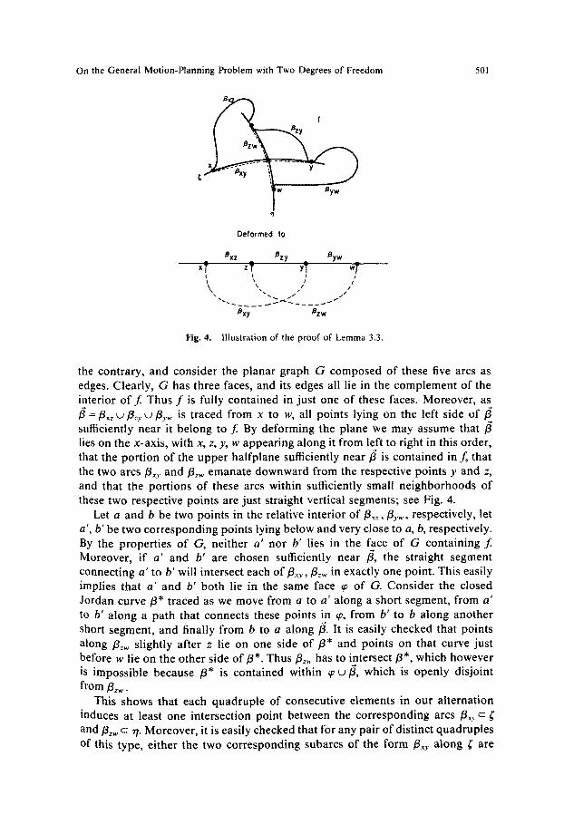
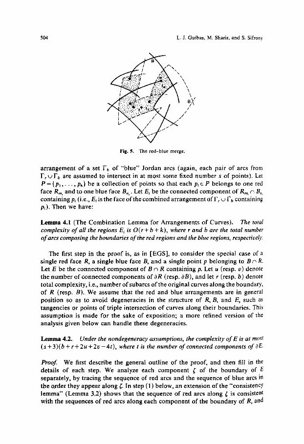
For technical reasons that are explained below, we extend this task as follows. Let P be the set containing x and all endpoints of curves of F which lie on the boundary of either R or B. Clearly, P contains at most 2n + 1 points. For each w e P let fw denote the connected component of R c~ B which contains w (these components are not necessarily distinct). Our task is now to calculate all these components (but produce each distinct component just once, even if it contains several points of P). We refer to this task as the red-blue merge. (The algorithm given below actually works in more general i ty--R and B can be the union of several connected regions, and P can be an arbitrary (finite) collection of points, as long as it contains all the endpoints of the curves in F which lie inside B, R as above.) We call the resulting components fw purple regions, as each of them is covered by both the red and the blue region. An illustration of this merge is shown in Fig. 5.

The major technical result on which our algorithm relies is that the overall complexity of these purple regions is small, so that it is not expensive to produce all of them. This is a consequence of the following extension of the combination lemma of [EGS]; it yields a somewhat weaker bound than that obtained in [EGS], but it suffices for our purpose.

4.1. The Combination Lemma for Arrangements of Curves

The combination lemma that we establish in this subsection is somewhat stronger than the version needed for our red-blue merge. We first introduce a few notations. Let R~ . . . . , R,, be a collection of m distinct faces in an arrangement of a collection F~ o f " r e d " Jordan arcs, and let B1, • • . , Bn be a similar collection of faces in an

504 L .J . Guibas , M. Sharir, and S. Sifrony

\ \ \ \

! /

/

Fig. 5. The r ed -b lue merge.

arrangement of a set Fb of "blue" Jordan arcs (again, each pair of arcs from Fr u Fb are assumed to intersect in at most some fixed number s of points). Let P = { P l , - - - , Pk} be a collection of points so that each p~ c P belongs to one red face R,,, and to one blue face Bn,. Let E~ be the connected component of R,,. c~ B,, containing p~ (i.e., E~ is the face of the combined arrangement ofFr u Fb containing p~). Then we have:

Lemma 4.1 (The Combination Lemma for Arrangements of Curves). The total complexity of all the regions E~ is O( r + b + k), where r and b are the total number o f arcs composing the boundaries o f the red regions and the blue regions, respectively.

The first step in the proof is, as in [EGS], to consider the special case of a single red face R, a single blue face B, and a single point p belonging to B c~ R. Let E be the connected component of B n R containing p. Let u (resp. v) denote the number of connected components of OR (resp. OB), and let r (resp. b) denote total complexity, i.e., number of subarcs of the original curves along the boundary, of R (resp. B). We assume that the red and blue arrangements are in general position so as to avoid degeneracies in the structure of R, B, and E, such as tangencies or points of triple intersection of curves along their boundaries. This assumption is made for the sake of exposition; a more refined version of the analysis given below can handle these degeneracies.

[,emma 4.2. Under the nondegeneracy assumptions, the complexity o r E is at most (s + 3)(b + r + 2u + 2v - 4t), where t is the number o f connected components of oE.

Proof We first describe the general outline of the proof, and then fill in the details of each step. We analyze each component ~ of the boundary of E separately, by tracing the sequence of red arcs and the sequence of blue arcs in the Qrder they appear along ~. In step (1) below, an extension of the "consistency lemma" (Lemma 3.2) shows that the sequence of red arcs along ~ is consistent with the sequences of red arcs along each component of the boundary of R, and


similarly for the blue sequence. We notice that a single red arc from R can be repeated several times along ~. However, in step (3) we argue that these repetitions must be interspersed with blue arcs which "advance" along the boundary of B. Although it is possible for a single red arc to be interspersed with a single blue arc for a while, after at most s +3 alternations at least one of them has to be replaced by another, as in the proof of Lemma 3.3. Another complication that can arise is that ~ may visit several components of the boundary of R or of B, so that some of them are visited more than once. We show in step (2) that the duplication of arcs along ~ that may result from this effect is only linear in the number of components. Altogether these arguments imply that the complexity of E is linear in the input size, as asserted in the lemma.

To begin the proof, let us fix a single component sr of aE, and assume, without loss of generality, that it is the exterior component. Trace ~ in, say, counterclockwise direction (with E lying to the left), and let S = S(= ( s~ , . . . , Sq) be the (circular) sequence of the subarcs of aR, aB as they appear along ~'. Clearly, the sum of the lengths of S s, over all connected portions ¢ of aE, is the complexity of E.

The proof consists of the following steps: (1) Let a be a subarc of, say, aR which appears along ¢. Let a l , a2 be two

connected portions of a c~ ¢ consecutive along a, such that when a is traversed with R lying to its left, al precedes a2. It follows from Lemma 3.2 that a~ and a2 are also adjacent along ~', in the strong sense that the portion of ¢ between a~ and a2 does not intersect the connected component of aR containing a.

We use the notation "the portion of S between si and sj" to mean the subsequence (si+l . . . . , sj_~) if i < j , or the subsequence (si+l, •. •, Sq, s ~ , . . . , sj_~) i f j < i. The property stated above then amounts to saying that if si = s t are two consecutive appearances of some red arc a in S, with the first appe, arance preceding the second one along a, then either the portion of S between s~ and sj consists of blue arcs exclusively, or, if it contains red arcs at all, they must all belong to other components of oR.

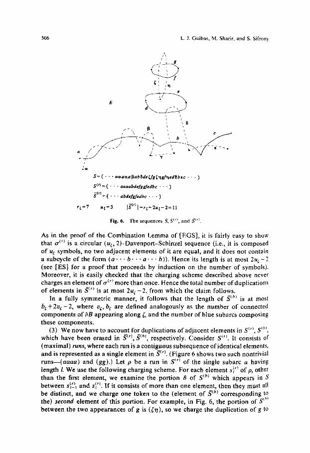
(2) Let S (r) be the (circular) subsequence of S obtained by deleting from S all the blue subarcs, and let S(r) be the sequence obtained from S (r) by further deleting, from left to right, each element which becomes equal to the element immediately preceding it. The sequences S ~b) and gcb) are defined symmetrically for the blue parts of S. See Fig. 6.

We claim that g(r) is of length at most r~+2u~-2, where u s is the number of distinct connected components of OR appearing along ~', and r s is the total number of red subarcs composing these u s components.

(Note that )"su¢ = u, and ~s rs = r, since no component of OR can appear along two distinct components of dE.)

To prove the claim, assume a is a red subarc appearing more than once in S(~). By (1), all elements of S(~) lying between two consecutive appearances ~I~), gJr) of a (arranged in this order along a) must belong to other components of OR. We charge the second appearance of a to the component of oR containing glr+)~. Let o "(r) be the (circular) sequence of the connected components of OR in the order they appear along ~ (so that no two adjacent elements of tr (r) are equal).


/ ° \

! i

J~ i /

I

S = ( " . . a c t a a a [ 3 a b g d e ~ J & ~ , q g f ~ e d g b ~ c . . , )

S ( r ) = ( . . . a a a a b d e f s g ~ e d b c . . . )

"~o ( . . . a ~ e ] ~ e a ~ , e . . • )

r{=7 u ~ = 3 1$ "¢°l=r{+2u{-2=11

Fig. 6. The sequences S, S (~), and St~

As in the proof of the Combination Lemma of [EGS], it is fairly easy to show that cr ~r) is a circular (us, 2)-Davenport-Schinzel sequence (i.e., it is composed of uc symbols, no two adjacent elements of it are equal, and it does not contain a subeycle of the form ( a . • • b. • • a . • • b)). Hence its length is at most 2u~-2 (see [ES] for a proof that proceeds by induction on the number of symbols). Moreover, it is easily checked that the charging scheme described above never charges an element of or ~r) more than once. Hence the total number of duplications of elements in g~r) is at most 2u~-2 , from which the claim follows.

In a fully symmetric manner, it follows that the length of ~b) is at most b~+2vc-2 , where vg, be are defined analogously as the number of connected components of OB appearing along ~, and the number of blue subarcs composing these components.

(3) We now have to account for duplications of adjacent elements in S ~r~, S Ibm, which have been erased in ~r) , ~cb), respectively. Consider S ~ . It consists of (maximal) runs, where each run is a contiguous subsequence of identical elements, and is represented as a single element in S~). (Figure 6 shows two such nontrivial runs--(aaaa) and (gg).) Let p be a run in S ~) of the single subarc a having length/. We use the following charging scheme. For each element s~ "~ of p, other than the first element, we examine the portion ~ of S ~b) which appears in S between s~_)~ and s~ ~). If it consists of more than one element, then they must all be distinct, and we charge one token to the (element of g~b) corresponding to the) second element of this portion. For example, in Fig. 6, the portion of S ~b~ between the two appearances of g is (Oq), so we charge the duplication of g to


the corresponding element rl o f ~(b~. Otherwise 6 consists o f a single element (b) If s~ ~ :~ _(b) si . T ~j_~, then again we charge one token to the corresponding element

of g(bt Otherwise no charge is made. In Fig. 6, the run ( a a a a ) has the following portions o f S (b) between its e l e m e n t s ~ ( a ) , (at), and (/3). Thus the third element of this run does not cause any charge to be made; the fourth element charges/3 (in g~b)), and the second element charges a (assuming a does not appear again on dE before its displayed portion). We use a symmetric charging scheme to the runs o f S (b~.

Consider now the full sequence S. An element o f S is said to be charged if it is a charged element in either S(*~ or ~tb). It is easy to check that no element of S(') or o f ~q(h) is charged more than once, so the total number o f tokens charged is at most

I g(~'l + IS(b)l ~ r~ + b e + 2u~ + 2v~ - 4.

Consider a port ion S* of S between two consecutive charged elements si and sj. Assume that this port ion contains more than one element in some run, and assume that the r ightmost such duplicat ion occurs within a run o f some arc a in, say, S (r). (In Fig. 6, consider the port ion S* = ( a a a ) . ) Let Sk, = Sk2 = a be this r ightmost duplication. Since no charge was made within S*, there must occur a single blue arc a between Sk, and Sk2, which furthermore is not the first in a run of S (b). Let st, = st2 = a be the two consecutive occurrences o f a within its run in S (b) so that 12 = k l + 1 . I f s~, also lies within S*, then again we must have l~ = k~ - 1, so that there is a single appearance o f a between these two appearances o f a, and this appearance is also not the first in its run. Cont inuing backward in this manner, it is easily verified that either the first element o f the run o f a or the first element of the run o f a must lie outside (i.e., before) S*, and that a and a are the only elements being dupl icated in consecutive places in S (r) or in S (b) within S*. Now, as in Lemma 3.3, the max imum number o f alternations o f the arcs a and a along

is s + 3, so that at most s + 2 alternations can occur within S*. In other words, we have shown that the excess o f S ~r) and S (b) over ~q~r~ and

~(b~, between any two adjacent charged elements, is at most s + 2 . Since the number o f charged elements is at most r ~ + b ~ + 2 u ¢ + 2 v ~ - 4 , it follows that the total length o f S is at most ( s + 3 ) ( r ~ + b ¢ + 2 u ~ + 2 v ¢ - 4 ) . Summing over all componen t s ~ o f OE, we obtain that its total complexi ty is at most (s + 3 ) ( r + b + 2u + 2 v - 4t) , as asserted. [ ]

Remark. Compar ing our analysis with that of the Combina t ion Lemma of [EGS] , we see that our b o u n d is not the best possible, at least for the case o f straight segments. It would be nice to sharpen our bound , if possible. However , our result implies that the complexi ty o f E is O ( r + b) , which is sufficient for our purposes.

Proof o f the Combina t ion L e m m a . The p roof is a fairly straightforward (and SOmewhat simplified) adapta t ion o f the p roof o f the combinat ion lemma for line segments given in lEGS] . For the sake o f completeness we describe the modified


proof with some detail. Fix a blue face B = B j which contains k i of the given points, say P l , . . . , Pk,. Let ~'l . . . . , ~1~ be the distinct connected components of 8B. For each of these points p~ let E~ denote the connected component of B c~ R,, which contains Pi, as defined above. Traverse each ~,~ and partition it into connected portions 8 so that each such portion intersects the boundary of only a single region Ei (and so that two adjacent portions intersect distinct such regions); note that in general the endpoints o f the portions 8 are not uniquely defined. We define a plane embedding of a planar graph G as follows. The vertices of G are the points p i , . . . , Pk, and additional l~ points ql . . . . , qt,, so that qi lies inside the connected component Hi of R 2 - B whose common boundary with B is ~i- For each portion 8 lying on some ~,, and intersecting some OEi, we add the edge (q,,,,p~) to G, and draw it by taking an arbitrary point in /~ c~OEi and connect it to p~ within E~ and to qm within Hm. The connectedness of each E~ and each Hm implies, as in [EGS], that we can draw all edges of G so that they do not cross one another. It follows from the definition of the portions 8 that in this embedding of G each face is bounded by at least three edges (note that G can have multiple edges between a pair of vertices). Thus by Euler's formula the number of edges in G, and thus the number of portions 8, is at mo~t 3(kj +/s). Figure 7, borrowed from [EGS], illustrates these arguments for the case of segments.

We next define, for each p~, a modified "b lue- red" region B* containing p~ as follows. I f R = R,, does not intersect OB at all, then we take B* = R. Otherwise we start at some point z on OB nOE~, and traverse the portion B of OB containing z (as defined in the preceding paragraph), with B lying to the left, until its last

i / "X "" 5 : :

/- \ ; .~. , ~ : ~ .~ ./ ,, /', I , . ' . , ' ,

/ ~'* / /1 |

-- / , , £ } .-.',.,

Fig. 7. Bounding the number of boundary portions using planarity.


Fig. 8. A "'blue-red" region B*.

intersection with OE~. Then we turn along OR into B and follow OR until its next intersection with OB. Since this intersection necessarily lies in aE~, we have landed on another portion S' ofaB which intersects aE~, and we follow 8' in the direction which keeps B to our left, until its last intersection with OE~, and continue this way until we get back to the starting point z. This yields one component of the boundary of the desired blue-red region B*. I f in this process we have not encountered all portions 8 of OB intersecting aE~, we pick another starting point on one of the portions we have missed, and repeat the tracing from that point. Finally, we add as components of aB* all components of aR which bound Ei but which are not intersected by aB at all (and are thus contained in the interior of B). Tracing all components of the boundary of OB* in this way yields a well-defined connected region bounded between these boundaries. Figure 8 shows an example of such a blue-red region.

It is easily checked that B* contains Ei and is contained in B. We define, in a completely symmetric manner, a modified " red-b lue" region R* around each pi. It follows that the connected component of B* n R* which contains p~ is exactly E , Moreover, assuming that no two points p , pj give rise to the same intersection face E, it is easy to check that aB* n Ej = OR* n Ej = O for any i # j . In other words, no arc of B* or of R* can appear on the boundary of another E~ (with Ej lying on the same side of that arc).

We are now in a position to apply Lemma 4.2. Let

b~ = the number of blue arcs of B*, r~ = the number of red arcs of R*, ui = the number of connected components of OB*, and v~ = the number of connected components of OR*.

By construction, all such components actually appear along aE~. Since each arc of OE~ is either a portion of a blue arc of B* or a portion of a red arc of R*, a slight modification of the proof of Lemma 4.2 (in which we only need to account for duplications of blue arcs of B* and of red arcs of R*) implies that the COmplexity of E~ is at most O(b~ + r~ + u~ + v~). Summing these inequalities over

510 L .J . Guibas , M. Sharir, and S. Sifrony

all points p,-, we conclude that the overall complexity of the regions Ei is at most

To bound Y.i hi, consider all blue-red regions B* contained in one original blue region Bj. Then ~p, cB, bi is bounded by the number of arcs of Bj plus a term proportional to the number of subarcs 8 into which aB) is partitioned. By the preceding argument, this additional term is O(k~ + !i) where k~ is the number of points p~ in B~, and lj is the number of connected components of OBj. We thus obtain, summing over all blue faces Bj,

~ b i=O kj+ . i I j = l

But ~ kj = k, and the total number of components of the blue faces is clearly bounded by their total complexity b. Hence

b, = O(b+ k). (ii) i

Repeating this counting for the red faces we obtain

r, = O(r+ k). (iii) i

Finally, ~ u~ (and ~ v~) can be bounded in a similar manner, noting that for each original blue face B~, the sum )~p,~B, u~ is bounded by lj plus the number of subarcs 6 along OBj, so that

• j i j = l

and similarly

~. v, = O(r+ k). (v) i

[3 Combining inequalities (i)-(v) completes the proof of the lemma.

4.2. The Red-Blue Merge

We now continue the description of our red-blue merge. Let ~r be the total number of vertices in the purple regions. The combination lemma, Lemma 4.1, implies that zr = O ( b + r + n ) = O(b+r) .

To facilitate our merge, we require certain information to be precomputed and available for each collection. Specifically, we require that the red region R be subdivided into x-monotone subregions by drawing vertical rays up and down from each point w in P n R, till they meet an edge of R (we call the resulting vertical segment through w the red vertical divider at w, and denote it by p(W)). It is easily checked that this does produce a decomposition of R as desired. See


p(w)

/

Fig. 9. Vertical dividers.

Fig. 9 for an illustration. Similar partitioning is required for the blue region, using blue vertical dividers (denoted as /3(w)), thereby obtaining a similar collection of blue x-monotone subregions.

These monotone decompositions of the red and blue regions are easy to obtain using a straightforward vertical line sweeping, in time O((b + r) log(b + r)). Note that a particular monotone subregion may terminate on the left or the right either because of a point of P, or because of a locally x-extremal vertex of the corresponding region. Our algorithm will produce a similar partitioning of the purple regions into monotone subregions, which we call the purple subregions.

We calculate the purple subregions by sweeping with a straight line. Notice that purple subregions start or end at x-coordinates associated with either a point of P, or with an x-extremum of the red or blue region, or with a red-blue intersection. In a left-to-right sweep we discover the portion of each purple subregion that is to the right of the leftmost point in P giving rise to it. Then afterward, in a right-to-left sweep, we get the portion of each purple subregion to the left of the rightmost point in P giving rise to it. Together, the two sweeps discover all the purple subregions.

Our algorithm will thus also attempt to construct purple regions incident to each blue or red endpoint (provided that the endpoint is also contained in the opposite-colored region--otherwise no such purple region is to be generated), even though such a purple region might not belong to the desired purple component f= fx . That is, some of these purple subregions might be disconnected from f (see Fig. 5 for an example). Intuitively, the reason for calculating these extra purple subregions is that we do not know a priori the shape o f fx , which may be very "wiggly." If we use only the point x to "trigger" the generation of purple subregions, we may need to sweep back and forth many times until we obtain the entire fx. However, using all endpoints of the red and blue arcs as triggering events is easily seen to yield, in just two sweeps as above, all the subregions of which fx is composed, and, as noted, perhaps a few extra subregions


as well. However, we will be able to detect all spurious subregions at the end of the algorithm, as follows. Consider the graph whose nodes are the final purple subregions, and whose edges connect pairs of purple regions adjacent along some vertical divider. Then a simple breadth-first search on this graph, starting from the purple subregion that contains x, will yield the desired component f ; all the unreachable purple subregions will simply be discarded. (Note also that the size of the additional "fake" purple regions is at most O(b + r) as follows easily from Lemma 4.1.)

We describe below only the left-to-right sweeping step; the right-to-left is symmetric. We start this sweep by constructing a priority queue, ordered by x-coordinate, which contains all the vertices appearing along the boundaries of the given red and blue regions, together with the point x. We sweep over the red and blue subregions separately, and at the same time will also sweep over the purple subregions, and detect (portions of) them as we sweep. We speak of the red, blue, and purple planes, respectively. The purpose of these separate sweeps is to avoid having to process "uninteresting" red-blue intersections, i.e., intersections which do not occur along the boundary of a purple region.

Every time we encounter a point p of P, we start one or two new purple subregions in the purple plane. At such an event we create, for each new purple region, two new purple "scouts": the upper scout and the lower scout. It is the job of these two scouts to walk along the upper and lower boundaries of the new purple regions, respectively. We describe the behavior of the upper scout u of one such region; the lower scouts behave symmetrically. See Fig. 10,

The upper scout u starts on a red or blue arc, as determined by the closest of the upper endpoints of the vertical dividers p(p),/3(p). The scout u moves right along that arc following the sweep line, but it needs to watch out for certain events that might influence the upper purple boundary of its region. Without loss of generality, we assume that u currently sits on a red arc. Figure 11 illustrates some aspects of the watching process.

The scout u has first to look up to the nearest blue arc/3 (note that since u is "purple," the entire vertical segment between u and/3 must be contained in

o

y j J

Fig. 10. Introduction of scouts.


U ~ O u

x

idle

/ /

/

/

I

(a)

V

V

u starts watching P

v starts watching

(b)

U

J

u

v starts watching [3

(c)

Fig. II .

u starts watching B

u - becomes idle

(d)

Several instances of the watching process.


B). The reason is that the blue boundary above u might at some future point drop below the red boundary the scout is currently following. If this were to occur, then u would have to follow the blue boundary, because now it delimits the purple subregion. However, there might be another scout v already watching that blue arc/3 from below. In that case only the highest of u and v needs to watch/3 from below: the other scout can rest, since it is certain that the higher scout is "protect ing" it from/3. See Fig. 1 l(a). In more technical detail, watching a blue arc /3 means timt u has to determine whether the arc p it lies on and 13 intersect to the right of the sweep line, and, if so, add the leftmost such intersection as an event into the priority queue of the sweep (each of these operations, except for the priority queue insertion, is assumed to take constant time in our model of computation). In addition, if the sweeping process reaches the right endpoint of either p or/3, which is not an endpoint of the whole curve (from F) containing that arc, u has to retest for a potential intersection between the new pair of arcs, and, if it exists, add the leftmost such intersection to the queue. When such a red-blue intersection is eventually swept across, u has to move to the blue arc t3, and to begin to watch the red boundary above it (starting with p). See Fig. l l (b) . (Note that the blue boundary above u, or the red boundary it currently follows, may also change discontinuously if the sweep reaches the endpoint of the corresponding full curve. When this happens, one of the things we have to do is to check whether the watching assignment of some purple scout has to change, and to inform the scout of this change. See below for more details.)

The scout u has also to look down to its lower partner and check for their (ieftmost) possible intersection (to the right of the sweepline), because when the two of them come together the current purple subregion must end. This, of course, might happen earlier, if another point of P is encountered between these scouts.

The key propert:¢ here is that each blue or red arc is watched (at any given time) by at most one upper scout and at most one lower scout, who sit on arcs of the opposite color. But these assignments of who watches over whom can change.

One way that can happen is that a purple region can end because its two purple scouts come together. This will occur, for instance, when the rightmost vertex of a red subregion lies inside a blue subregion. In this event, the two purple scouts of that purple subregion are eliminated. However, some transfer o f watching responsibility may now be indicated. I f the upper scout u was watching a blue arc/3, then we must consult the next upper purple scout down from u, say v. I f v is currently idle, because the next higher blue arc above v is the same arc/3 watched by u, then u transfers to v the responsibility of watching ft. See Fig. l l (c) . I f v is already watching another blue arc, then we leave it undisturbed, as its blue arc must be below/3.

Another way the two purple partner scouts can come together is when a purple region ends at a red-blue crossing. Any transfers of watching responsibility that need to happen now can be dealt in an entirely analogous way. I f a purple region ends because another point p of P appears between the scouts, then again the


two scouts are eliminated, but in this case they will generally be replaced by new scouts spawned by p.

The reassignment of watching responsibility that occurs when we sweep through a point p of P is, in more detail, as follows. At this time zero, one or two new purple subregions are created. Assume for simplicity that only one new subregion arises, and let u be its top scout. This scout u finds the opposite-colored arc e it has to watch by searching through the list of arcs of that color currently intersecting the sweepline (and represented as a balanced binary tree). But then u also has to consult the upper purple scout u* (resp. u-) lying directly above u (resp. below u). If u + is watching the same e (more precisely, if u + lies below e), then u remains idle. Otherwise u begins to watch e and checks whether u- is also watching e, in which case u- becomes idle. See Fig. l l (d) . Similar but somewhat modified actions are taken when two new purple regions are spawned at p.

In further detail, suppose p is an endpoint of a red original curve; then we check whether p also lies in the blue region B. If so, we start one or two new purple regions incident to p (and lying to its right), and proceed with scout creation and watching reassignments as above; otherwise no new purple region is to be generated at p. In either case, if the vertical divider p(p) extends both up and down from p (i.e., p is a point of "vertical tangency" on the boundary of its region), then some red boundaries currently watched by a purple scout may change discontinuously. For example, if the two red arcs e~, e 2 incident to p extend to the right of p (with e~ lying below e2), then we search through the list of purple regions along the sweepline to find the upper scout u lying directly below p, and, if it lies on a blue arc, tell u to start watching e~, unless it is watching a red arc lying below p. If u lies on a red arc, then if it is idle we leave it undisturbed; if it is watching a blue arc lying below p we again leave it undisturbed; however, if u watches a blue arc/3 above p, then it is easily checked that p must also lie within the blue region B, and consequently two new purple regions will be created at p, new purple scouts will be spawned along 81, e2, and the (upper) scout along el will relieve u from the responsibility of watching fl, as explained above. Similar or symmetric actions are taken in all the other subcases.

Finally, some transfer of watching may be required at a red-blue crossing lying, say, on the top boundary of some purple region. Suppose the corresponding top purple scout u was lying on a red arc p just before the intersection, and afterward it moves along a blue arc/3. As noted above, u now has to start watching p, but we also need to check whether the top purple scout v lying directly below u has to change the arc it is watching, or become idle. Details are similar to the cases considered above, and can be easily worked out by the reader.

Our scout watching scheme is designed in such a way that when a boundary of some purple subregion begins to traverse a new arc, only a constant number of scouts have to be told about it. This implies that handling such an event requires only a constant number of operations, including tree searches and priority queue updates, and thus takes only logarithmic time.


Note that this procedure not only produces the purple regions, but also their x-monotone decompositions into purple subregions, which will be handy for further processing. However, some preprocessing might still be required before subsequent merges (call them purple-violet) can be performed. This is because an endpoint p of some purple original curve may also lie within the violet region, in which case we will need to find the violet vertical divider at p, and this information in general is neither part of the "purple" data nor part of the "violet" data, and can be obtained only by combining information from these two collections prior to their merge.

Let us now analyze the complexity of this process. The purple scouts simply trace the boundaries of the purple regions. Each such scout needs to schedule into the priority queue possible intersection events between the arc it is currently sitting on, and the arc it is watching (including the possible intersection between the current top and bottom arcs of the same purple subregion). Note that new events are scheduled when we sweep either through a point in P, through a blue vertex, through a red vertex, or through a red-blue crossing (which is a vertex of a purple subregion). Moreover, at each such point only a constant number of new events are scheduled. Thus the total number of events ever scheduled is proportional to the total input and output size, which, by Lemma 4.1, is O(b + r). Thus each event costs O(log(b+r)) time to insert into (and delete from) the priority queue. The additional operations of our procedure involve updating the red, blue, and purple lists along the sweepline, of creating and eliminating scouts (i.e., purple subregions), and of reassigning watching responsibilities. It is plain that we need to perform only O(b+r) such operations, and that each can be carried out in O(log(b + r)) time (because the maximum size of the red, blue, and purple lists along the sweepline is at most O(b + r)). The final step of detecting "true" purple subregions (those that are connected to the "anchor" point x), and of eliminating the other subregions, can be done by a simple graph searching (as explained earlier) in time linear in the number of purple subregions produced by the algorithm, i.e., in O(b+r) time. Thus our procedure runs in overall time O((b + r) log(b + r)). Moreover, in our application each of the regions R and B is a single connected component in an arrangement of n/2 Jordan arcs (or curves), each pair of which intersect in at most s points. We have thus shown:

Theorem 4.3. Given two connected "red" and "blue" regions R, B, both containing a given point x, whose boundaries are composed respectively of r and b subarcs of some collection of Jordan arcs (or curves), no pair of which intersecting at more than s = O(1) points, we can calculate the connected component f of the intersection R n B which contains x, in time O((r+ b) log(r+ b)), under the assumptions made at the beginning of the section concerning the given curves and the model of computation.

The time bounds given above are for the merge step of our algorithm. Using Theorem 3.1, we thus obtain, by straightforward calculation.


Theorem 4.4. Given a collection F of n Jordan arcs (or curves), having the property that no pair of them intersect in more than s points, and also satisfying the conditions made above, we can calculate the connected component of A(F) containing a specified point x, in time O(A~+2(n) log 2 n) (or in time O(A~(n) log 2 n) for closed Jordan curves).

Remarks. (1) This result follows and extends the previous algorithm given in [EGS] for the case of line segments. It shows that the red-blue merge is a versatile technique of a purely topological nature, which can be applied to fairly general classes of curves.

(2) Our version of the combination lemma (Lemma 4.1) is weaker than the corresponding lemmas for lines or for line segments, as given in [EGS], in that the bound it produces involves the red and blue complexities r, b with coefficients greater than 1 (namely, s+3) . This does not allow us to apply the lemma in a repeated recursive fashion (as has been done in [EGS]) to obtain sharp upper bounds on the complexity of many connected components in an arrangement A(F) as above. However, assuming that a sharp bound on this complexity can be obtained by other means, our red-blue merge can be easily extended to obtain an algorithm for calculating m such components, each specified by a given point within it, in time comparable with their total worst-case complexity. Recently, [CEG*] have obtained sharp upper bounds for the complexity of m faces in arrangements of n circles, or of n unit circles, or of n pseudolines (i.e., x-monotone unbounded arcs, each pair of which intersects at most once). Using their bounds, we can obtain the following results (we omit details of the solutions of the resulting divide-and-conquer recurrences, which are based on random sampling of the given collection of curves, and are very similar to those obtained in [EGS]).

Corollary 4.5.

(a) We can calculate m distinct faces in an arrangement of n unit circles in (randomized) time O(m2/3-~ n2/3+2~ log n + n log 2 n) for any 8 > O.

(b) We can calculate m distinct faces in an arrangement of n arbitrary circles in (randomized) time O(m3/5-~ n4/5+2n log n + n log 2 n) for any 8 > O.

(c) We can calculate m distinct faces in an arrangement of n pseudolines (under an appropriate model of computation) in (randomized) time O(m2/3-g n 2/3+2~ log n + n log 2 n) for any 8 > O.

(3) Concerning lower bounds, it is easy to establish an f l(n log n) bound by reducing from sorting. We do not know of any larger lower bound. In particular, we pose it as an open problem whether a component of A(F) can be computed in time O(A~+2(n) log n). We note that an algorithm with such complexity exists for the calculation of the lower envelope of the arcs in F [At], [HS].

(4) If the collection F consists of n closed Jordan curves, then we can use our red-blue merge to calculate a single component of A(F) in time O(as(n) log 2 n), making use of the bound obtained in [SS5], as mentioned at the end of Section 3. In the special case s = 2, a simple adaptation of the algorithm in [KLPS] yields an algorithm with that complexity.


(5) Returning to the original motion-planning problem, the above procedure will yield a single connected component of FP, provided this component is fully contained in a single planar patch of the entire parametric space AP. If AP is not planar, and the desired component C which contains the initial placement Z "spills" over into more than one patch, we obtain C using the following technique. Let AP~,. . . , APq be the planar patches which compose AP, and assume that Z lies in AP1. We first calculate the component Co in AP~ containing Z. If Co does not reach the boundary of AP~, then C = Co. Otherwise, we also calculate all the unbounded components in each of the patches AP~. Assuming that the number of patches is constant, and that each of the constraint curves is broken into a constant number of connected subarcs, each lying within a single patch, it is easily checked that the total complexity of all unbounded components of the patches is O(As÷2(n)), and that they can all be calculated in time O(hs+2(n) log 2 n), using the above algorithm. The desired component C is easily seen to be the union of Co with certain portions of the unbounded components within the patches. More precisely, as Co reaches the boundary of APt, C extends into another patch, necessarily as a portion of the unbounded component within that patch; similar "propagat ion" of C into further patches continues until the whole of C is obtained. Clearly this tracing of C can be accomplished within the above time bound.

Let us discuss a few applications of our results to some specific motion-planning problems. As a first example, consider a line segment B = PQ free to rotate in three dimensions about its endpoint P which is fixed at the origin. The motion of B clearly has two degrees of freedom, and, assuming the obstacles that B has to avoid are all polyhedral (with a total of n edges), we easily check that any pair of constraint curves intersect in at most s = 1 point. Thus the complexity of a single component of FP is O(na(n)), and can be calculated in time O(not(n) log 2 n). (Note that in this case AP can be represented as the surface of a sphere in three dimensions, or, alternatively, as the union of two planar patches.)

As a second example, let B be a two-link arm PQR moving in the plane (amidst polygonal obstacles) with the point P fixed at the origin. Here AP can be represented by a torus, or by a union of four planar patches. By using tan(0J2), tan(02/2) as the system parameters, it is easily checked that each constraint curve is algebraic of (at most) fourth degree. Moreover, it can be shown that each pair of constraint curves intersect in at most s = 2 points (on a single patch). It follows that the complexity of a single component of FP is O ( ) t a ( n ) ) , and that it can be calculated in time O(A4(n) log 2 n).

As a final example, consider the problem of coordinated motion planning for two "planar Stanford arms" [FWY], [SSi], where each arm is a straight segment PiQi free to translate through a fixed point Ci and also rotate about that point, for i = 1, 2. We consider a special case of coordinated motion, in which the two endpoints Q~, Q2 must be in contact with each other throughout the motion. This problem has been studied in [FWY], who gave an O(n 2 log n) algorithm (where


n is the total number of obstacle corners and edges). A recent result in [SSi] shows that the desired free space can be taken to be a single component in the intersection of the two 2-D configuration spaces of the two separate arms. Since each of these spaces has O(n) complexity [FWY], [SSi], a single application of our red-blue merge yields the desired space in time O(n log n).

5. Conclusion

The results obtained in this paper provide a satisfactory solution to the general motion-planning problem with two degrees of freedom. The problem is in a much more confused state, however, when we consider problems with three degrees of freedom. There, under assumptions similar to those made above, the complexity of the entire FP is O ( n 3) in general, although there are certain favorable cases in which the complexity reduces to quadratic or near-quadratic. For example, for a line segment moving in the plane amidst polygonal obstacles, the complexity of FP is O(n 2) [LS2], [SIS]. For a convex k-gon moving in a similar environment, the complexity of FP is O(knA6(kn)) [KS2]. (See also [Si2] for a few other favorable instances of this sort.) However, for a nonconvex (e.g., an L-shaped) polygon, the complexity of FP can be f~(n3), as is easily checked. As above, we would like to conjecture that a single connected component of FP, which is all we really need to compute, will have smaller, e.g., near-quadratic, complexity. However, this appears to be a much harder problem, and is largely open. Some progress was recently made on this problem for the special case in which the surface patches bounding FP are n triangles in 3-space. It was shown in [PSI that the complexity of a single component of their complement is at most O(n3-1/49). This was improved in [AS] to O(n7/30l(n) 2/3 log 4/3 n) , where this also bounds the total complexity of all nonconvex components. Another simplified case is where instead of calculating the boundary of a component of the complement of the given constraint surfaces, we only want to calculate their upper or lower envelope, i.e., the portions of these surfaces seen from a point at infinity in the direction of the positive or negative z-axis. For triangles, it was shown in [PS] that the complexity of their upper envelope is O(n2a(n)), and that this bound is worst-case optimal. However, for arbitrary surfaces, even in this restricted problem subcubic upper bounds are not known, except for a few special cases noted in [SS5].

References

[ASS] P. Agarwal, M. Sharir, and P. Shor, Sharp upper and lower bounds for the length of general Davenport-Schinzel sequences, Tech. Rept. 332, Comput. Science Dept., Courant Institute, New York, 1987. (To appear in J. Combin. Theory Set. A.)

[AgS] P. Agarwal and M. Sharir, Red-blue intersection detection algorithms, with applications to motion planning and collision detection, Proc. 4th ACM Syrup. on Computational Geometry, 1988, pp. 70-80.


[AS]

[At]

[BO]

[BZ]

ICE]

[CG]

[c1]

[CEG*]

[EG]

[EGHI*]

[EGH2*]

[EGP*]

[EGS]

[ES]

[FWY]

[HS]

[Ha] [KSI]

[KS2]

[KLPS]

[LS1]

[LS2]

[Mul]

B. Aronov and M. Sharir, Triangles in space, or: Building (and analyzing) castles in the air, Proc. 4th A C M Syrup. on Computational Geometry, 1988, pp. 381-391. (Also to appear in Combinatorica.) M. Atallah, Dynamic computational geometry, Proc. 24th IEEE Symp. on Foundations of Computer Science, 1983, pp. 92-99. Also in Comput. Math~ AppL !1 (1985), pp. 1171- 1181. J. L. Bentley and T. Ottmann, Algorithm for reporting and counting geometric intersections, IEEE Trans. Comput. 28 (1979), pp. 643-647. B. Bhattacharya and J. Zorbas, Solving the two-dimensional findpath problem using a line-triangle representation of the robot, J. Algorithms 9 (1988), pp. 449-469. B. Chazelle and H. Edelsbrunner, An optimal algorithm for intersecting line segments in the plane, Proc. 29th IEEE Syrup. on Foundations of Computer Science, 1988, pp. 590-600. B. Chazelle and L. Guibas, Visibility and intersection problems in plane geometry, Proc. 1st ACM Symp. on Computational Geometry, 1985, pp. 135-146. K. Clarkson, Applications of random sampling in computational geometry, I I, Proc. 4th A C M Symp. on Computational Geometry, 1988, pp. 1-11. K. Clarkson, H. Edelsbrunner, L. Guibas, M. Sharir, and E. Welzl, Combinatorial complexity bounds for arrangements of curves and surfaces, Proc. 29th IEEE Syrup. on Foundations of Computer Science, 1988, pp. 568-579. H. Edelsbrunner and L. Guibas, Topologically sweeping an arrangement, Proc. 18th ACM Symposium on Theory of Computing, 1986, pp. 389-403. H. Edelsbrunner, L. Guibas, J. Hershberger, R. Seidel, M. Sharir, J. Snoeyink, and E. Welzl, Implicitly representing arrangements of lines or segments, Discrete Comput. Geom. (1989), this issue, pp. 433-436. H. Edelsbrunner, L. Guibas, J. Hershberger, J. Pach, R. Pollack, R. Seidel, M. Sharir, and J. Snoeyink, On arrangements of Jordan arcs with three intersections per pair, Proc. 4th A C M Syrup. on Computational Geometry, 1988, pp. 258-265. H. Edelsbrunner, L. Guibas, J. Pach, R. Pollack, R. Seidel, and M. Sharir, Arrangements of arcs in the plane: Topology, combinatorics, and algorithms, Proc. 15th Int. Colloq. on Automata, Languages and Programming, 1988, pp. 214-229. H. Edelsbrunner, L. Guibas, and M. Sharir, The complexity of many faces in arrangements of lines or of segments, Proc. 4th A C M Syrup. on Computational Geometry, 1988, pp. 44-55. H. Edelsbrunner and M. Sharir, The maximum number of ways to stab n disjoint convex sets in the plane is 2 n - 2 , Tech. Rept. 281, Comput. Sci. Dept., Courant Institute, New York, 1987 (to appear in Discrete Comput. Geom.). S. Fortune, G. Wilfong, and C. Yap, Coordinated motion of two robot arms, Proc. IEEE Conf. on Robotics and Automation, 1986, pp. 1216-1223. S. Hart and M. Sharir, Nonlinearity of Davenport-Schinzel sequences and of generalized path compression schemes, Combinatorica 6 ( 1986 ), pp. 151-177. R. Hartshorne, Algebraic Geometry, Springer-Verlag, New York., 1977. K. Kedem and M. Sharir, Efficient algorithm for planning translational collision-free motion of a convex polygonal object in 2-dimensional space amidst polygonal obstacles, Proc. 1st A C M Syrup. on Computational Geometry, 1985, pp. 75-80. K. Kedem and M. Sharir, An efficient motion-planning algorithm for a convex polygonal object in two-dimensional polygonal space, to appear in Discrete Comput. Geom. K. Kedem, R. Livne, J. Path, and M. Sharir, On the union of Jordan regions and collision-free translational motion amidst polygonal obstacles, Discrete Comput. Geom. 1 (1986), pp. 59-71. D. Leven and M. Sharir, An efficient and simple motion-planning algorithm for a ladder moving in two-dimensional space amidst polygonal barriers, J. Algorithms 8 (1987), pp. 192-215. D. Leven and M. Sharir, Planning a purely translational motion of a convex object in two-dimensional space using generalized Voronoi diagrams, Discrete Comput. Geom. 2 (1987), pp. 9-31. K. Mulmuley, A fast planar partition algorithm, 1, Proc. 29th IEEE Syrup. on Foundatwns o f Computer Science, 1988, pp. 590-600.


[Mu2] K. Mutmutey, A fast planar partition algorithm, II, Proc. 5th ACMSymp. on Computational Geometry, 1989, pp. 33-43.

[OSY1] C. O'Dfinlaing, M. Sharir, and C. Yap, Generalized Voronoi diagrams for a ladder: I. Topological considerations, Comm. Pure AppL Math. 39 (1986), pp. 423-483.

[OSY2] C. O'Dfinlaing, M. Sharir, and C. Yap, Generalized Voronoi diagrams for a ladder: II. Efficient construction of the diagram, Algorithmica 2 (1987), pp. 29-57.

[OY] C. 6'Dtlnlaing and C. Yap, A "retraction" method for planning the motion of a disc, J. Algorithms 6 (1985), pp. 104-111.

[PSI J. Pach and M. Sharir, The upper envelope of piecewise linear functions and the boundary of a region enclosed by convex plates: combinatorial analysis, Discrete Comput. Geom. 4 (1989), pp. 291-309,

[PSS] R. Pollack, M. Sharir, and S. Sifrony, Separating two simple polygons by a sequence of translations, Discrete Comput. Geom. 3 (1988), pp. 123-136.

[SS1] J. T. Schwartz and M. Sharir, On the piano movers' problem: I. The case of a rigid polygonal body moving amidst polygonal barriers, Comm. Pure Appl. Math. 36 (1983), pp. 345-398.

[SS2] J. T. Schwartz and M. Sharir, On the piano movers' problem: II. General techniques for calculating topological properties of real algebraic manifolds, Adv. in Appl. Math. 4 (1983), pp. 298-351.

[SS3] J. T. Schwartz and M. Sharir, On the piano movers' problem: III. Coordinating the motion of several independent bodies: The special case of circular bodies moving amidst polygonal barriers, lnternat. J. Robotics Res. 2 (1983) (3), pp. 46-75.

[SS4] J. T. Schwartz and M. Sharir, On the piano movers' problem: V. The case of a rod moving in 3-D space amidst polyhedral obstacles, Comm. Pure AppL Math. 37 (1984), pp. 815-848.

[SS5] J. T. Schwartz and M. Sharir, On the two-dimensional Davenport-Schinzel problem, Tech. Rept. 193 (revised), Comput. Sci. Dept., Courant Institute, New York, t987. (To appear in J. Symbolic Computation.)

[SA] M. Sharir and E. Ariel-Sheffi, On the piano movers' problem: IV. Various decomposable two-dimensional motion-planning problems, Comm. PureAppL Math. 37 (1984), pp. 479- 493.

[SSi] M. Sharir and S. Sifrony, Coordinated motion planning for two independent robots, Proc. 4th A C M Syrup. on Computational Geometry, 1988, pp. 319-328.

[Sh] P. Shor, Geometric realizations of superlinear Davenport-Schinzel sequences, in prepar- ation.

[Sil] S. Sifrony, Efficient algorithms for motion-planning problems in robotics, Ph.D. Disserta- tion, Tel Aviv University, 1989.

[Si2] S. Sifrony, Efficient algorithms for motion planning of certain spatial 3-DOF manipulator arms, manuscript, 1989.

[SIS] S. Sifrony and M. Sharir, A new efficient motion-planning algorithm for a rod in 2-D polygonal space, Algorithmica 2 (1987), pp. 367-402.

[WS] A. Wiernik and M. Sharir, Planar realization of nonlinear Davenport-Schinzel sequences by segments, Discrete Comput. Geom. 3 (1988), pp. 15-47.

Received July 25, 1988, and in revised form March 22, 1989.

Date post:	18-Mar-2020
Category:	Documents
Upload:	others
View:	3 times
Download:	0 times

On the General Motion-Planning Problem with Two Degrees …On the General Motion-Planning Problem...

Documents