SCHOOL OF ECONOMICS AND FINANCE Discussion Paper 2013-11 On the Impact of the Global Financial Crisis on the Euro Area Xiaoli He, Jan P.A.M. Jacobs, Gerard H. Kuper and Jenny E. Ligthart ISSN 1443-8593 ISBN 978-1-86295-919-4
Transcript
SCHOOL OF ECONOMICS AND FINANCE
Discussion Paper 2013-11
On the Impact of the Global Financial Crisis on the Euro Area
Xiaoli He, Jan P.A.M. Jacobs, Gerard H. Kuper and Jenny E. Ligthart
ISSN 1443-8593 ISBN 978-1-86295-919-4
On the Impact of the Global Financial Crisison the Euro Area
Xiaoli HeUniversity of Groningen
Jan P.A.M. Jacobs1
University of Groningen, UTAS, CAMA and CIRANO
Gerard H. KuperUniversity of Groningen
Jenny E. Ligthart2
Tilburg University, University of Groningen, CAMA and CESifo
September 2013
1Send correspondence to: J.P.A.M. Jacobs, Faculty of Economics and Business, University ofGroningen, P.O. Box 800, 9700 AV Groningen, [email protected]
2A few days after this paper was presented at the Workshop on Business Fluctuations andInternational Transmission of Shocks, Kobe University, Kobe, Japan, November 2012, our col-league, co-author and dear friend Jenny Ligthart passed away. This paper could never have beenwritten without her, and the final result would definitely have been better with her input. Wethank Adrian Pagan and participants of the Workshop, in particular Tsutomu Miyagawa, forhelpful comments.
Abstract
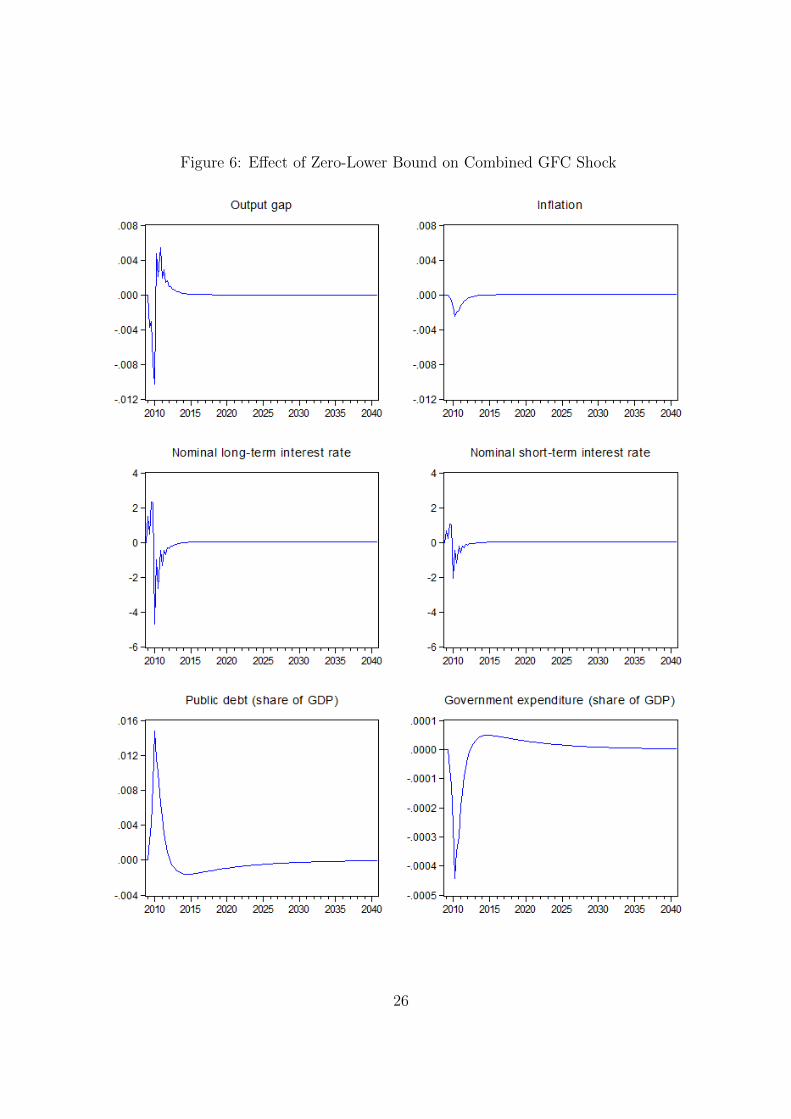
This paper analyses the impact of the Global Financial Crisis on the Euro area utilizing asimple dynamic macroeconomic model with interaction between monetary policy and fiscalpolicy. The model consists of an IS curve, a Phillips curve, a term structure relation, a debtaccumulation equation and a Taylor monetary policy rule supplemented with a Zero LowerBound, and a fiscal policy rule. The model is calibrated/estimated for EU-16 countriesfor the period 1980Q1–2009Q4. The impact of the Global Financial Crisis is studied bymeans of impulse responses following a combined, prolonged aggregate demand and publicdebt shock. The simulation mimicking the GFC turns out to work fairly well. However,the required size of the shock is quite large.
Keywords: Global Financial Crisis, euro area, monetary policy, fiscal policy, New Neoclas-sical Synthesis model, Zero Lower Bound
JEL-code: C51, C52, E63
1 Introduction
The Global Financial Crisis (GFC) in 2007–2008 has had an huge impact on the euro area,
and until now the recovery is still not under way. Even worse, the European sovereign debt
crisis triggered by the GFC resulted in large difficulties for several Euro area countries to
refinance their government debt. Starting in late 2009, the Greek government began having
problems to meet its debt obligations, and in April 2010 Greece government bonds were
downgraded to the status of junk bonds, which led to panic in European and even global
financial markets. Despite the fact euro area member states and the IMF provided one
hundred and ten billion euro bail-out loans to Greece in May 2010, the debt crisis did not
stop and even spread to other euro area countries such as Ireland, Portugal and Spain.
Since the Maastricht Treaty was signed by the member countries of the European Union
(EU), individual euro area countries design independent macroeconomic (fiscal) policies.
This makes dealing with the current economic condition in the Euro area quite complicated.
This paper focuses on the impact of the Global Financial Crisis on the euro area. We
utilize a simple dynamic macroeconomic model, which is heavily inspired by Kirsanova,
Stehn and Vines (2005; henceforth KSV), who focus on the interaction between monetary
and fiscal policy of a single economy against shocks in a dynamic setting. They set up a five-
equation model consisting of a dynamic and linearized IS equation with Blanchard-Yaari
consumers (Yaari, 1965; Blanchard, 1985), a Phillips curve (Bean, 1998), a linearized debt
accumulation equation and two policy rules, a Taylor-like monetary policy rule (Taylor,
1995) and a fiscal policy rule. Both monetary and fiscal policy makers are benevolent;
monetary policy makers will make monetary policy do nearly all of the stabilization.
One of the features of the model is the interaction of monetary and fiscal policy. Al-
most all existing models concerning the interaction between monetary and fiscal policy
only include the short-term interest rate and basic macro-founded household consumption
1
structure. However, the long-term interest rate is the relevant interest rate for financing
government debt, and microeconomic elements such as real estate values, stock returns
and living expectation can also considerably influence household consumption behaviour.
Therefore, Jacobs, Kuper and Ligthart (2010; henceforth JKL) add a term structure to
the macro model KSV to link the long-term interest rate to the short-term interest rate.
JKL claim that including a term structure equation in the model can improve the
estimates of fluctuations of macro variables, which is supported by several studies. For
instance, Estrella and Mishkin (1997) state that a yield curve can serve as a efficient
method to guide monetary policy making in Euro area, which is supported by Camarero,
Ordonez and Tamarit (2005). Furthermore, Bekaert, Cho and Moreno (2010) show that
the inclusion of a term structure can improve the effectiveness of generating large and
significant estimates of the Phillips curve and real interest rate response parameters. On
the other hand, Rudebusch, Sack and Swanson (2007) argue that the model does not
improve by incorporating the term structure, but Berardi (2009) showes that the ability of
structural models with a term structure to forecast movements of macroeconomic variables
does not deteriorate. Rudebusch and Wu (2008) combine the finance literature of the term
structure with a macroeconomic description of the yield curve to allow for a bidirectional
feedback between factors that describe the term structure and macroeconomic variables.
To model the impact of the Global Financial Crisis, Lane and Milesi-Ferretti (2010)
focus on the changes in values of macro variables before and after the crisis. It turns out
that after the crisis, there is a considerable decrease in domestic demand and the growth
rate, and an increase in public debt. Moreover, financial topics related to the crisis are
also frequently analysed. For example, Shahrokhi (2011) emphasises the cause of the crisis
and the future of capitalism, while Bracke and Fidora (2012) focus on the macro-financial
environment of the global economy after the crisis. Also, Moshirian (2011) shows that
since the global financial framework is not perfectly integrated, cross border regulatory
2
arbitrage still exists even after the Global Financial Crises. In our paper, we model the
Global Financial Crisis through a combination of shocks, and study the responses.
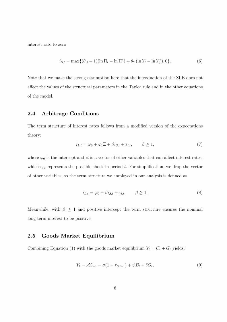
We introduce a Zero-Lower-Bound (ZLB) in the monetary policy rule. When confronted
with a financial crisis, the most common reaction of developed countries’ central banks is to
cut nominal short-term interest rates considerably. Belke and Klose (2012) show that both
the US Federal Reserve (Fed) and the European Central Bank (ECB) employ this method
in reaction to the GFC. However, nominal interest rates cannot become negative, and ZLB
frequently serves as a binding constraint on monetary policy with low inflation targets.
Reifschneider and Williams (2000) indicate that with a 2% inflation rate, ZLB works as a
binding constraint about 10% of the time in the simulations of the Fed Board’s FRB/US
model. Also, Williams (2010) shows that after the GFC the ZLB has become a binding
constraint on monetary policy in most industrial countries with monetary policy rates
below 1%. As a result, with already low nominal short-term interest rate, the room left
for the ECB to further cut short-term interest rates is limited, and conventional monetary
policies are no longer effective (Belke and Klose 2012, Gerlach and Lewis 2010).
The paper is structured as follows. Section 2 introduces the basic analytical framework
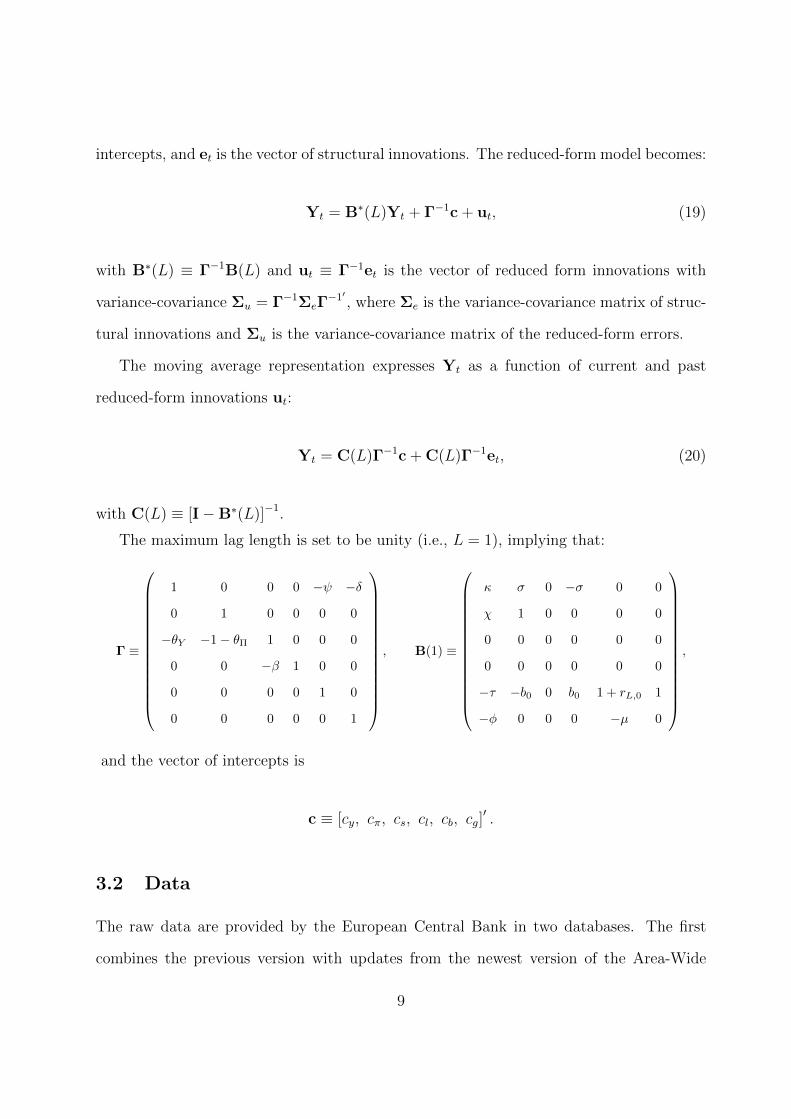
used in this paper. Section 3 presents the econometric model, data, calibration of the
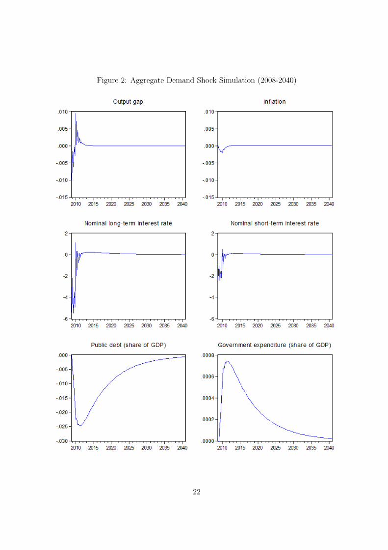
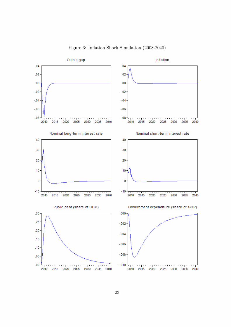
parameters and stability analysis. Section 4 shows single shock simulations in Section 4.1
and the outcomes of the combined shock, the GFC scenario, in Section 4.2. Section 5
concludes.
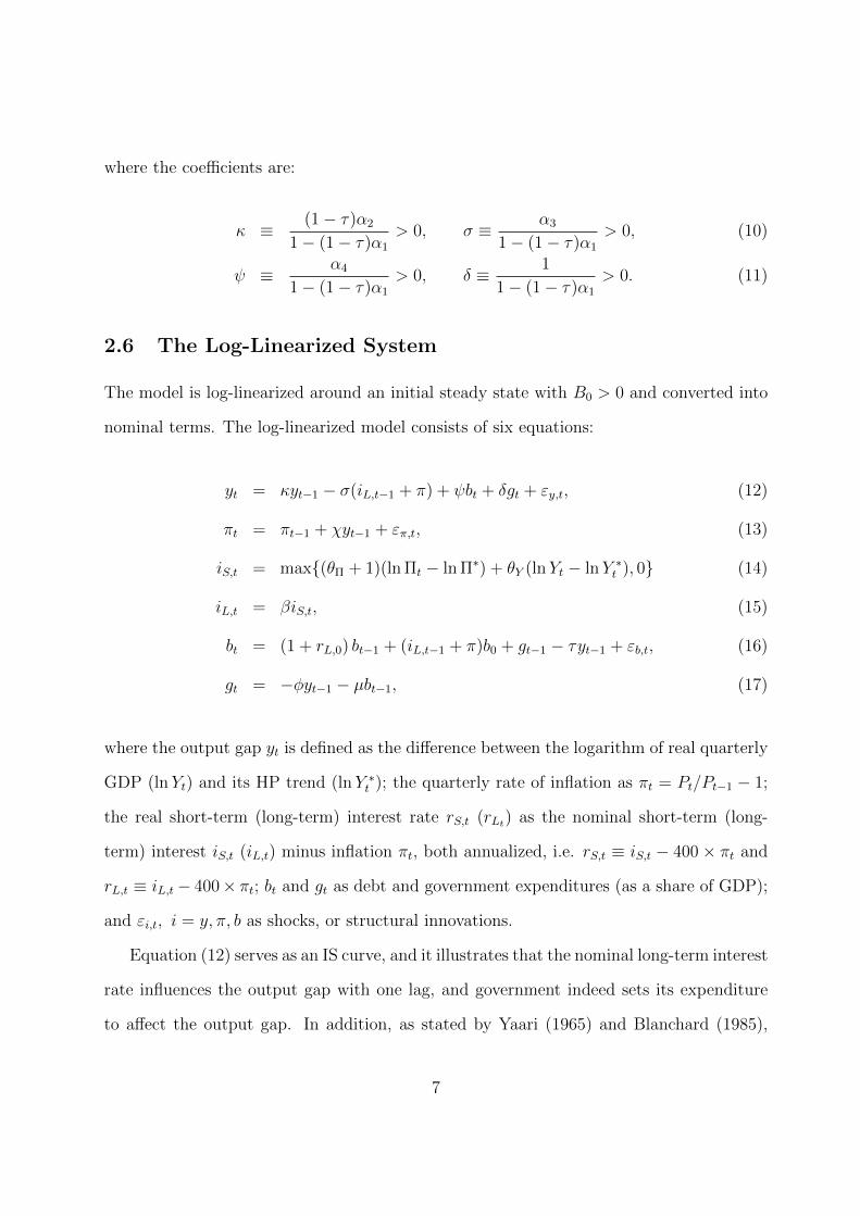
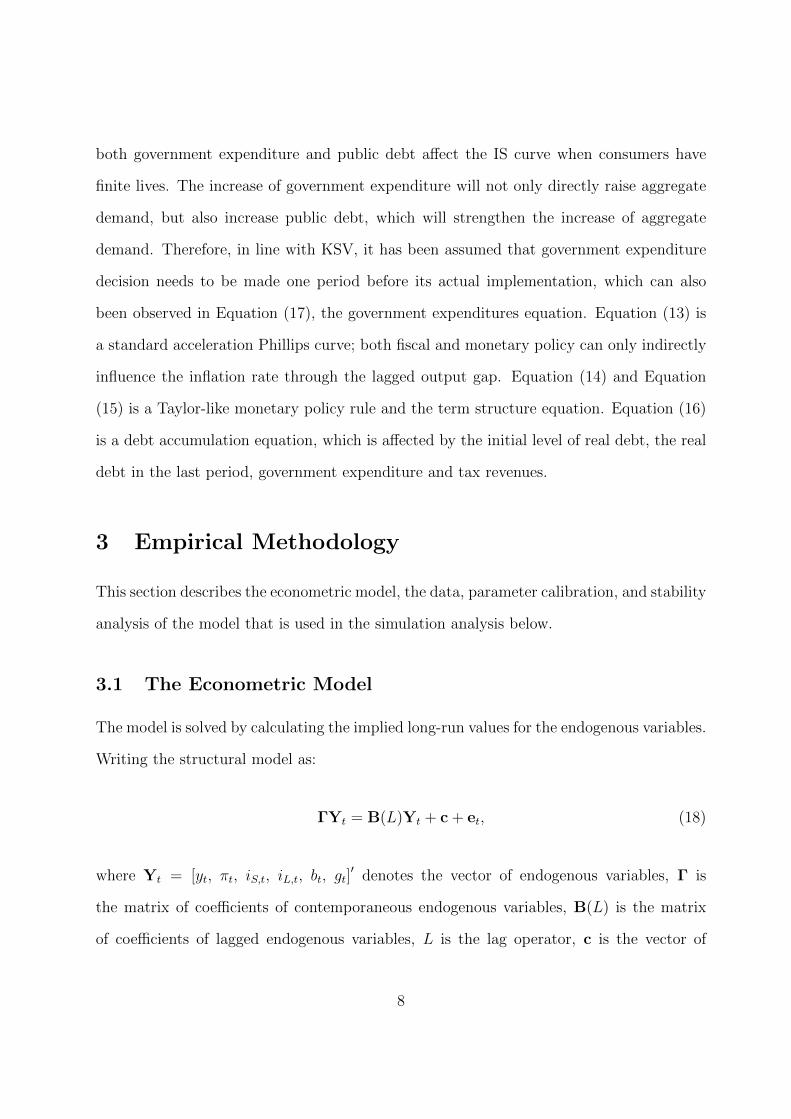
2 The Model
This section first provides the design of our model, which extends the macro model of KSV
with a term structure relationship. The model is a simple dynamic macroeconomic model
3
of a closed economy with Blanchard-Yaari consumers, rule of thumb price setting firms,
and a government.
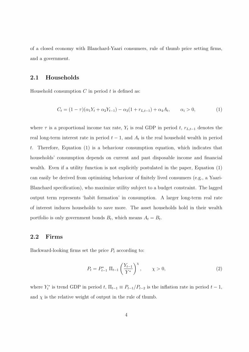
2.1 Households
Household consumption C in period t is defined as:
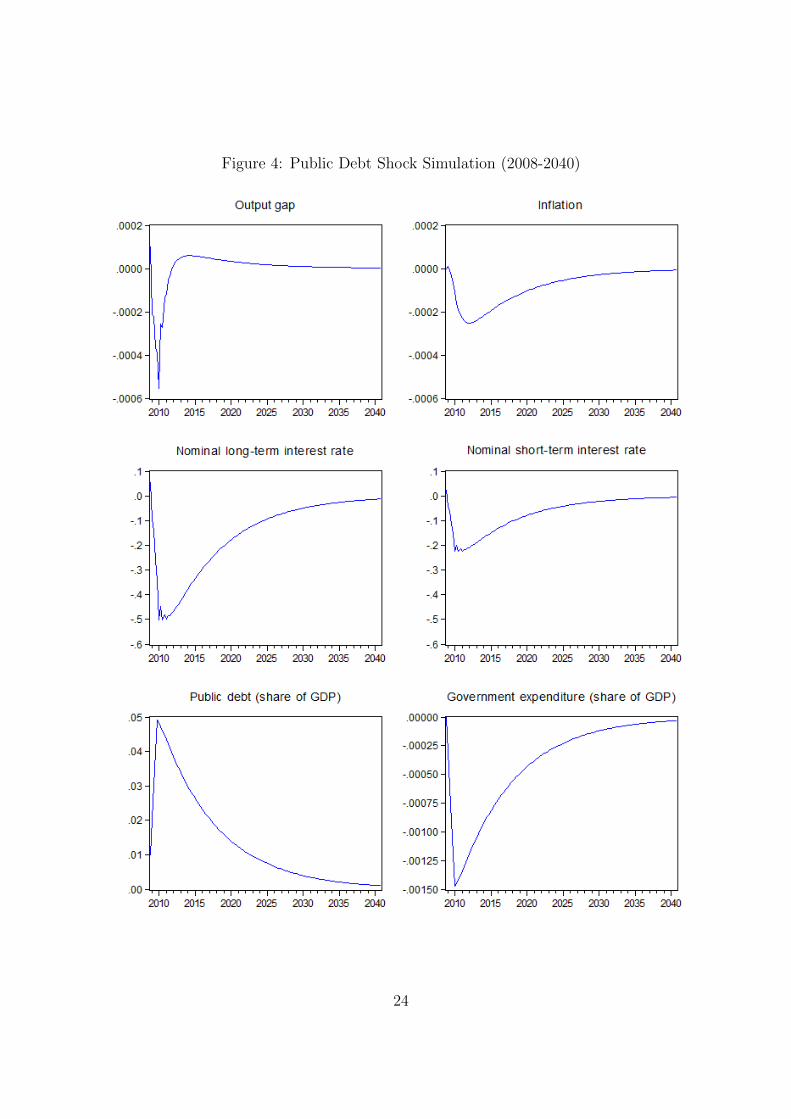
Figure 4: Public Debt Shock Simulation (2008-2040)
24
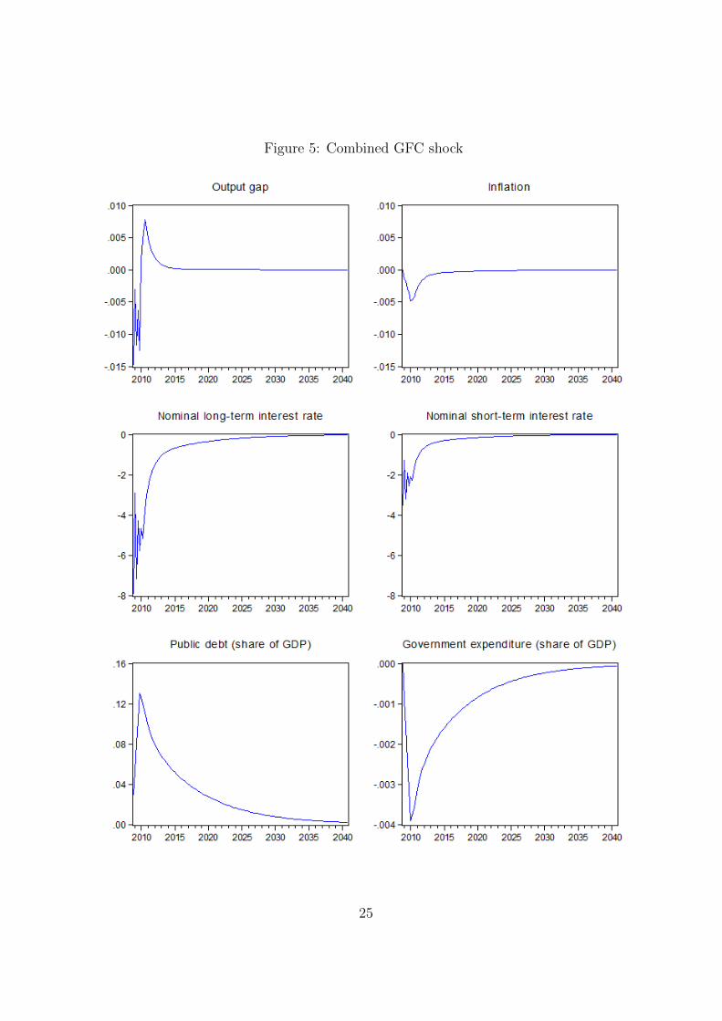
Figure 5: Combined GFC shock
25
Figure 6: Effect of Zero-Lower Bound on Combined GFC Shock
26
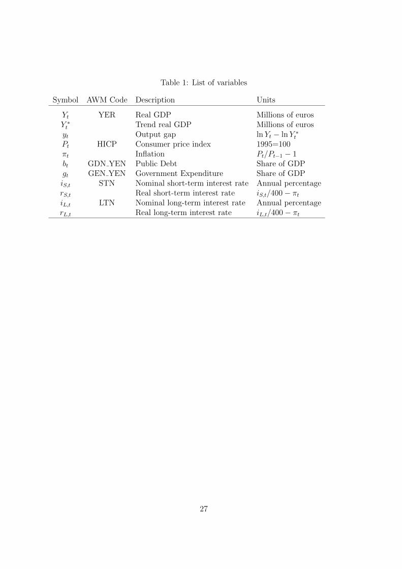
Table 1: List of variables
Symbol AWM Code Description Units
Yt YER Real GDP Millions of eurosY ∗t Trend real GDP Millions of eurosyt Output gap lnYt − lnY ∗tPt HICP Consumer price index 1995=100πt Inflation Pt/Pt−1 − 1bt GDN YEN Public Debt Share of GDPgt GEN YEN Government Expenditure Share of GDPiS,t STN Nominal short-term interest rate Annual percentagerS,t Real short-term interest rate iS,t/400− πtiL,t LTN Nominal long-term interest rate Annual percentagerL,t Real long-term interest rate iL,t/400− πt
27
School of Economics and Finance Discussion Papers
2013-15 Equity market Contagion during the Global Financial Crisis: Evidence from the World’s Eight Largest Economies, Mardi Dungey and Dinesh Gajurel
2013-14 A Survey of Research into Broker Identity and Limit Order Book, Thu Phuong Pham and P Joakim Westerholm
2013-13 Broker ID Transparency and Price Impact of Trades: Evidence from the Korean Exchange, Thu Phuong Pham
2013-12 An International Trend in Market Design: Endogenous Effects of Limit Order Book Transparency on Volatility, Spreads, depth and Volume, Thu Phuong Pham and P Joakim Westerholm
2013-11 On the Impact of the Global Financial Crisis on the Euro Area, Xiaoli He, Jan PAM Jacobs, Gerald H Kuper and Jenny E Ligthart
2013-10 International Transmissions to Australia: The Roles of the US and Euro Area, Mardi Dungey, Denise Osborn and Mala Raghavan
2013-09 Are Per Capita CO2 Emissions Increasing Among OECD Countries? A Test of Trends and Breaks, Satoshi Yamazaki, Jing Tian and Firmin Doko Tchatoka
2013-08 Commodity Prices and BRIC and G3 Liquidity: A SFAVEC Approach, Ronald A Ratti and Joaquin L Vespignani
2013-07 Chinese Resource Demand and the Natural Resource Supplier Mardi Dungy, Renée Fry-McKibbin and Verity Linehan
2013-06 Not All International Monetary Shocks are Alike for the Japanese Economy, Joaquin L Vespignani and Ronald A Ratti
2013-05 On Bootstrap Validity for Specification Tests with Weak Instruments, Firmin Doko Tchatoka
2013-04 Chinese Monetary Expansion and the US Economy, Joaquin L Vespignani and Ronald A Ratti
2013-03 International Monetary Transmission to the Euro Area: Evidence from the US, Japan and China,
Joaquin L Vespignani and Ronald A Ratti
2013-02 The impact of jumps and thin trading on realized hedge ratios? Mardi Dungey, Olan T. Henry, Lyudmyla Hvozdyk
2013-01 Why crude oil prices are high when global activity is weak?, Ronald A Rattia and Joaquin L Vespignani
Copies of the above mentioned papers and a list of previous years’ papers are available from our home site at http://www.utas.edu.au/economics‐finance/research/