On the Kolmogorov Complexity ofContinuous Real Functions

Amin FarjudianDivision of Computer Science

University of Nottingham Ningbo, China

Abstract

Kolmogorov complexity was originally defined for finitely-representable objects.Later, the definition was extended to real numbers based on the asymptotic be-haviour of the sequence of the Kolmogorov complexities of the finitely-represent-able objects—such as rational numbers—used to approximate them.

This idea will be taken further here by extending the definition to continuousfunctions over real numbers, based on the fact that every continuous real functioncan be represented as the limit of a sequence of finitely-representable enclosures,such as polynomials with rational coefficients.

Based on this definition, we will prove that for any growth rate imaginable,there are real functions whose Kolmogorov complexities have higher growth rates.In fact, using the concept of prevalence, we will prove that ‘almost every’ continu-ous real function has such a high-growth Kolmogorov complexity. An asymptoticbound on the Kolmogorov complexities of total single-valued computable realfunctions will be presented as well.

Keywords: Kolmogorov Complexity, Algorithmic Randomness, ComputableAnalysis, Domain Theory, Measure Theory, Prevalence2000 MSC: 68Q30, 03D32, 28C20, 06B35

1. Introduction

In computer science, Kolmogorov complexity of an object provides a measureof the complexity of its description, hence the alternative name descriptive com-

Email address: Amin.Farjudian@nottingham.edu.cn (Amin Farjudian)URL: www.cs.nott.ac.uk/˜avf (Amin Farjudian)

Preprint submitted to Elsevier November 18, 2012

plexity. Although commonly known as Kolmogorov complexity, Solomonoff [21,22] was the first to develop the concept, for the purpose of studying the complexityof finite objects, such as the finite sequences of binary digits.

This concept of complexity has indeed been extended and studied over non-finite objects such as real numbers, regarding which, there are at least two mainapproaches in the literature: one based on the real Turing machine (RTM) ofBlum, Shub, and Smale [3]; and the other based on an effective setting, such asthe Type-2 Theory of Effectivity (TTE) of Weihrauch [24].

A real Turing machine is conceptually very similar to an ordinary Turing ma-chine, except that each of its registers is capable of holding the exact value of areal number at any time, and the machine is capable of carrying out arithmeticoperations on real numbers in unit time. Montana and Pardo [17] and Ziegler andKoolen [25] have studied Kolmogorov complexity over sequences of real numbersbased on the theory of real Turing machines. This approach is very elegant buttoo abstract to address the issue of effective representation of real numbers.

Type-2 theory of effectivity is another framework for studying computabilityover real numbers, within which the issue of effective representation is addressed.Hence, it provides a theoretical foundation for exact real computation [7, 8, 9,24]. In this framework, each ideal object (such as a non-finitely-representablereal number, function, manifold, etc.) is represented as the limit of a sequence offinitely-representable approximations.

As an example, consider the case of real numbers. Each real number canbe represented as the limit of a sequence of rational numbers. Another choicefor a basis of representation of real numbers is the set of arbitrary precisionfloating point numbers [10, 16, 19]. In fact, it is in this setting that the Kol-mogorov complexity of real numbers has been studied by Cai and Hartmanis [4]and Staiger [23].

In a sound and complete exact framework, the correct result of any computa-tion must be obtainable to within any accuracy that is demanded. For instance, inone viable protocol one could represent accuracy using integers, and interpret anaccuracy n as ‘being within the radius 2−n of the exact result’. In general, the con-crete indicator of accuracy is arbitrary. Nonetheless, the expectation is that with‘higher’ accuracy demanded, one needs more computational resources to providea satisfying answer to the querying party.

The inspiration for the framework of this paper comes mainly from the workof Cai and Hartmanis [4]. Every real number x ∈ [0, 1] can be approximated bya sequence 〈xi〉i∈N of arbitrary precision binary floating point numbers in [0, 1], insuch a way that:

2

1. each xn has a binary representation of the form rxn = 0.dxn1 dxn

2 . . . dxnn where

∀i ∈ N : dxni ∈ {0, 1}. In other words, each xn has at least one representation

of maximum length 2 + n. If we ignore the common leading “0.” prefix,then we can say that each xn has a representation of maximum length n.

2. ∀n ∈ N : | x − xn | < 2−n.

In a fixed language, for each n ∈ N, there may be a description of xn with astring of characters which is shorter than its binary expansion. Therefore, for eachreal number x ∈ [0, 1] and each n ∈ N, there exists a rational number xn ∈ [0, 1]which has a description of length at most n and satisfies | x − xn | < 2−n. If we letK(xn) denote the length of the shortest possible description of any such xn thenK(xn) ≤ n. For the real number x, the Kolmogorov complexity KR(x) can bedefined as:

KR(x) B12

(lim inf

n→∞

K(xn)n

+ lim supn→∞

K(xn)n

)It should be clear that ∀x ∈ [0, 1] : 0 ≤ KR(x) ≤ 1. Cai and Hartmanis [4] provethat:

(i) For Lebesgue-almost every x in [0, 1]: KR(x) = 1.

(ii) For every t ∈ [0, 1], the set K−1R (t) is uncountable and has Hausdorff dimen-

sion t.

(iii) The graph of KR is a fractal.

We try to address the cost of representation of functions by extending the def-inition of Kolmogorov complexity to the set C[0, 1] of continuous real functionsfrom [0, 1] to R. The main result of this paper states that no matter what rateof growth one considers, ‘almost all’ functions in the Banach space C[0, 1] haveKolmogorov complexities with higher growth rates. As such, this result can beregarded as an extension of item (i) to the case of the function space C[0, 1].

The extension of the concept of Kolmogorov complexity to the function spacessuch as C[0, 1] or C(2N) has already been studied in contexts different to that ofours. Barmpalias et al. [2] have studied the concept over the function space C(2N)in the context of descriptive set theory. Fouche [11, 12] has extensively studiedthis subject in the context of Brownian motion.

3

2. Kolmogorov complexity of a continuous real function

In what follows, by representation of the functions in C[0, 1] we mean therepresentation of each such element as the limit of a (not necessarily computable)sequence of finitely-representable objects. Domain theory [1, 6, 8, 13] providesa suitable setting for this purpose. Of course, the actual structure that we intro-duce will not be a domain, but concepts such as approximation will be developedin accordance with domain theory. To start, we use enclosures to approximatefunctions:

Definition 1 ([ f, g]: function enclosure).

1. For f , g ∈ R[0,1] we define the function enclosure [ f , g] by

[ f , g] B{h ∈ R[0,1] ∀x ∈ [0, 1] : f (x) ≤ h(x) ≤ g(x)

}(Obviously if ∃x0 ∈ [0, 1] : g(x0) < f (x0) then [ f , g] will be empty.)

2. The function f (respectively g) is called the lower boundary (respectivelyupper boundary) of the enclosure [ f , g].

3. Enclosures H1 and H2 are said to be consistent if H1 ∩ H2 , ∅. Otherwise,they are said to be inconsistent.

Furthermore, tighter enclosures provide better approximations of a function. Thisis expressed using the width of an enclosure:

Definition 2 (w: width operator). Consider f , g ∈ C[0, 1]. For the enclosure [ f , g]the width is defined as w([ f , g]) B max {g(t) − f (t) t ∈ [0, 1]}.

Note that w([ f , g]) is well defined as [0, 1] is compact and both f and g areassumed to be continuous.

Definition 3 (Γ(h): graph of a function enclosure). Let h = [ f , g] be an enclosure.By the graph of h we mean the set of points in [0, 1] × R lying between the graphsof its lower and upper boundaries. Set theoretically, this is just the union of allfunctions in the enclosure, i. e. Γ(h) B ∪h.

The set of continuous-function enclosures under the reverse inclusion forms aposet:

4

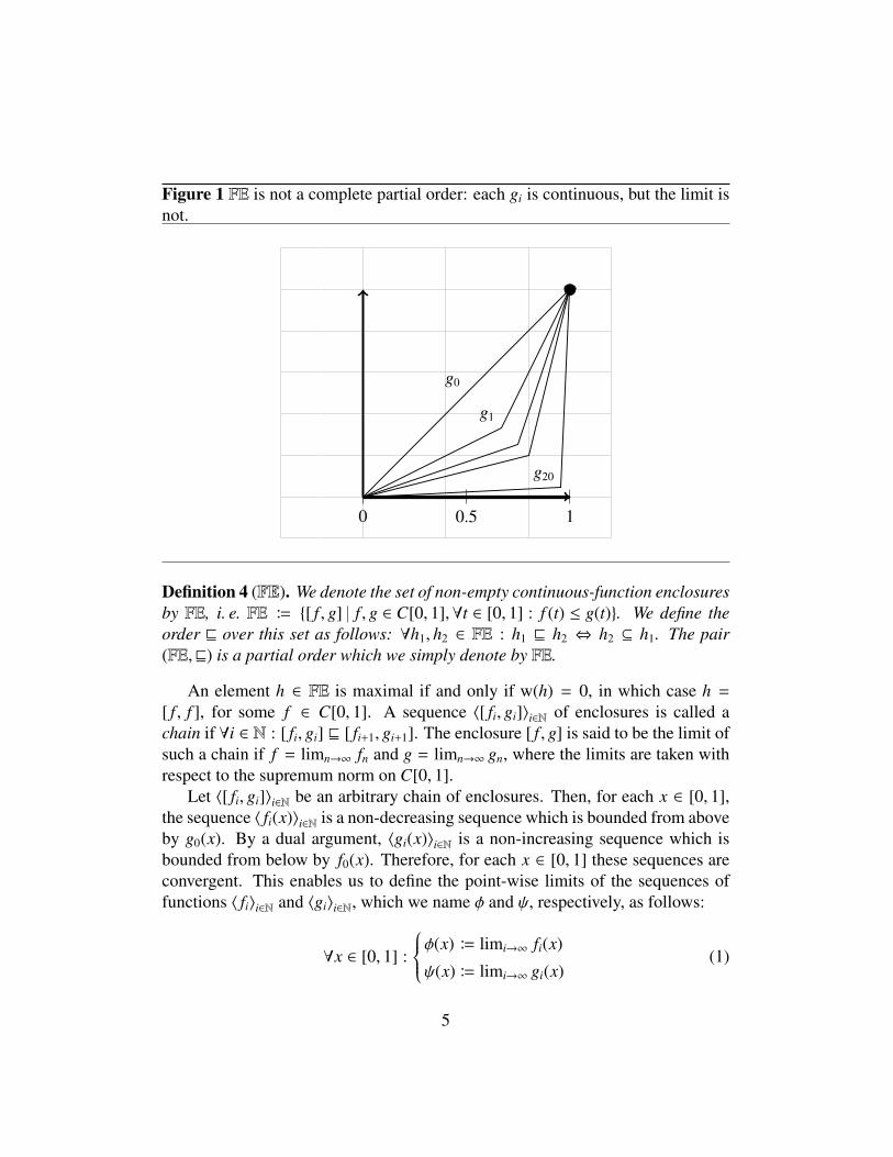
Figure 1 FE is not a complete partial order: each gi is continuous, but the limit isnot.

0 0.5 1

g0

g1

g20

Definition 4 (FE). We denote the set of non-empty continuous-function enclosuresby FE, i. e. FE B {[ f , g] f , g ∈ C[0, 1],∀t ∈ [0, 1] : f (t) ≤ g(t)}. We define theorder v over this set as follows: ∀h1, h2 ∈ FE : h1 v h2 ⇔ h2 ⊆ h1. The pair(FE,v) is a partial order which we simply denote by FE.

An element h ∈ FE is maximal if and only if w(h) = 0, in which case h =

[ f , f ], for some f ∈ C[0, 1]. A sequence 〈[ fi, gi]〉i∈N of enclosures is called achain if ∀i ∈ N : [ fi, gi] v [ fi+1, gi+1]. The enclosure [ f , g] is said to be the limit ofsuch a chain if f = limn→∞ fn and g = limn→∞ gn, where the limits are taken withrespect to the supremum norm on C[0, 1].

Let 〈[ fi, gi]〉i∈N be an arbitrary chain of enclosures. Then, for each x ∈ [0, 1],the sequence 〈 fi(x)〉i∈N is a non-decreasing sequence which is bounded from aboveby g0(x). By a dual argument, 〈gi(x)〉i∈N is a non-increasing sequence which isbounded from below by f0(x). Therefore, for each x ∈ [0, 1] these sequences areconvergent. This enables us to define the point-wise limits of the sequences offunctions 〈 fi〉i∈N and 〈gi〉i∈N, which we name φ and ψ, respectively, as follows:

∀x ∈ [0, 1] :

φ(x) B limi→∞ fi(x)

ψ(x) B limi→∞ gi(x)(1)

5

The functions φ, ψ : [0, 1] → R are well-defined but not necessarily contin-uous. As an example, take the chain {[ fi, gi] i ∈ N} defined (for all i ∈ N andx ∈ [0, 1]) by fi(x) = 0 and

gi(x) =

x/(i + 1) if 0 ≤ x ≤ 1 − 1/(i + 2)

(i + 1)x − i if 1 − 1/(i + 2) ≤ x ≤ 1

Figure 1 on the preceding page depicts this chain which is made up of piece-wise linear enclosures.1 For an example with polynomial enclosures, one canconsider gi(x) = xi. It should be clear that in both cases ∀i ∈ N : [ fi, gi] v[ fi+1, gi+1], but the limit of 〈gi〉i∈N is the non-continuous function

ψ(x) =

{0 if x ∈ [0, 1)1 if x = 1

Nonetheless, if {hi i ∈ N} is a chain such that limi→∞w(hi) = 0, then the chainhas a limit in FE. To see this, let us assume that for each i ∈ N, hi = [ fi, gi] anddefine φ and ψ as in (1) on the previous page. The assumption limi→∞w(hi) = 0implies that φ = ψ. Thus, we only need to show that (say) ψ is continuous, whichwe will prove by contradiction.

Assume that ψ is discontinuous at some point z ∈ [0, 1]. Without loss ofgenerality, we assume that for some ε > 0, there exists a sequence of points 〈zi〉i∈N

such that:2

(limi→∞

zi = z) ∧ (∀i ∈ N : ψ(zi) − ψ(z) > ε) (2)

As ψ(z) = limi→∞ gi(z), we can find an n0 ∈ N such that ∀n ≥ n0 : | gn(z) − ψ(z) | <ε/4. Because 〈gi(z)〉i∈N is a non-increasing sequence, we have ∀n ≥ n0 : gn(z) −ψ(z) < ε/4. Let us fix n at n0 for now and use the continuity of gn0 to derive:

gn0(z) − ψ(z) < ε/4(continuity of gn0 at z) ⇒ lim

i→∞gn0(zi) − ψ(z) < ε/4

(property of limit) ⇒ ∃i0 ∈ N : ∀i ≥ i0 : gn0(zi) < ψ(z) + ε/4(By (2) and fixing i at i0) ⇒ gn0(zi0) < ψ(zi0) − ε + ε/4 < ψ(zi0) − 3ε/4

(As ε > 0) ⇒ gn0(zi0) < ψ(zi0)

1Strictly speaking, each boundary is a piece-wise affine function consisting of affine segments.Nonetheless, to make the material more accessible, we will keep using the terms ‘piece-wiselinear’ functions and ‘linear’ segments, as they are well-established terms in literature.

2The case of (∀i ∈ N : ψ(z) − ψ(zi) > ε) can be dealt with in a similar manner.

6

which is a contradiction as by definition, at every point x ∈ [0, 1] the value of eachgi must be greater than or equal to that of ψ, i. e. gn0(zi0) ≥ ψ(zi0).

We summarise these results in the following proposition:

Proposition 5. The partial order FE is not complete, i. e. it is not closed un-der the limit operator over chains. However, if {hi i ∈ N} is a chain such thatlimi→∞w(hi) = 0, then the chain has a limit in FE.

The condition limi→∞w(hi) = 0 is sufficient but not necessary for convergencein FE. For instance, the sequence 〈[ fi, gi]〉i∈N in which

∀i ∈ N : ∀x ∈ [0, 1] :

fi(x) = 0

gi(x) = x(i + 2)/(i + 1)

is a chain which converges to the enclosure [λx.0, λx.x] whose width is 1.Basic concepts in function enclosure arithmetic [5, 20] will be used in this

paper. The intuition behind this arithmetic is very simple as operators on functionsmimic operators of ordinary interval arithmetic [18]. For instance, addition can beeasily overloaded with function enclosures as in [ f1, g1] + [ f2, g2] B [ f1 + f2, g1 +

g2]. With other operations (such as ×, etc.), a bit of tweaking is needed, similar tothe case of ordinary interval arithmetic.

It is possible to be more practically minded and restrict oneself to a set offinitely-representable function enclosures, and still be able to approximate everyfunction in C[0, 1]. For instance, one may consider the set of enclosures [ f , g]such that f and g are polynomials with rational coefficients.

Of course objects are finitely-representable only relative to some specific lan-guage L ⊆ Σ∗, for some alphabet Σ. To make the presentation easier, we assumethat our alphabet is rich enough to include:

• 0 and 1;

• some appropriate symbols for arithmetic operators;

• some appropriate symbols for forming lists, pairs and lambda expressions.

All of these can be encoded by appropriate Turing machines, and as we studyasymptotic behaviour, the inclusion or exclusion of these elements in Σ will notaffect our results. Nonetheless, it is crucial that we keep the alphabet finite, as wewill see from the proof of Proposition 10.

7

We say that an enclosure h is approximated by another enclosure g if g isfinitely-representable and g v h.3 A countable set B of finitely-representableenclosures is called a basis for FE if each h ∈ FE is the limit of a chain 〈hi〉i∈N ofelements in B. Examples of bases are:

• the set of polynomials with rational coefficients;

• the set of continuous piecewise-linear functions, where the end-points ofeach linear segment have rational coordinates.

Now let B be a basis for FE. We call ρ : N → B a binary representation off ∈ C[0, 1] if ∀n ∈ N : (ρ(n) v [ f , f ]) ∧ (w(ρ(n)) < 2−n).

Remark 6. All of our results can be easily generalised to any base. Thus, to savespace, we will refer to binary representations simply as representations.

Notation 1. We reserve the notation K(x) to denote the Kolmogorov complexity ofany finitely-representable object x. This includes objects such as integer numbers,finite strings over a finite alphabet, arbitrary-precision floating-point numbers,finitely-representable function enclosures, and the like.

Proposition 7. For every function f ∈ C[0, 1] there exists a representation f of fof minimal Kolmogorov complexity, i. e. for any other representation of f such asρ : N→ B:

∀n ∈ N : K( f (n)) ≤ K(ρ(n))

Proof. Assume that B is enumerated as 〈hi〉i∈N. In order to define f over a cer-tain n ∈ N, first let Xn be those elements of B that approximate f and have widthsmaller than 2−n, i. e. Xn B {h ∈ B h v [ f , f ],w(h) < 2−n} and consider the setK(Xn) = {K(h) h ∈ Xn} which is the image of Xn under K. This is a subset of N,hence it has a least element n0. All that remains is to assign to f (n) one of the ele-ments in K−1(n0), for instance, the one with the smallest index in the enumeration〈hi〉i∈N of B. �

Definition 8 (optimal representation). The representation f as in Proposition 7 iscalled an optimal representation of the function f .

3Note that our definition of approximation is different from the way-below relation used indomain theory [1, Definition 2.2.1]. In particular, in our framework any finitely-representableenclosure g approximates itself.

8

Definition 9 (KC( f )). Let f : N→ B be an optimal representation of f ∈ C[0, 1].The Kolmogorov complexity function of f is defined as:

KC( f ) : N→ Nn 7→ K( f (n))

We will consider the asymptotic growth of KC( f ) for functions in C[0, 1]. Thisway we can study the set of functions f for which KC( f ) is bounded in some way,e. g. by some polynomial, or some exponential function.

We will first prove in Proposition 10 that there are functions in C[0, 1] witharbitrarily fast-growth Kolmogorov complexity. In the proof we seem to go tosome length to manufacture ‘one’ such function. But, then—as is usually the casein mathematics—in Section 5 we will show that in fact ‘almost all’ functions inC[0, 1] have this property.

Proposition 10. For any given θ : N → N, there exists a function f in C[0, 1]whose Kolmogorov complexity is above θ over infinitely many points. In otherwords:

∀m ∈ N : ∃n ≥ m : KC( f ) (n) ≥ θ(n)

Proof. Appendix A on page 15. �

For instance, in Proposition 10, by taking θ(n) to be:

1. 2n, one can show that there exists a real function f ∈ C[0, 1] whose Kol-mogorov complexity KC( f ) is not dominated by any polynomial.

2. n!, one can show that there exists a real function f ∈ C[0, 1] whose Kol-mogorov complexity KC( f ) is not dominated by any exponential function.

3. Invariant ideals

Consider the poset (NN,�) in which � is the pointwise ordering on functions:f � g⇔ ∀n ∈ N : f (n) ≤ g(n), and define the operators ∨,∧ : NN ×NN → NN by( f∨g)(n) = max( f (n), g(n)) and ( f∧g)(n) = min( f (n), g(n)). This way one obtainsa lattice, in which certain ideals (and their complements) are of interest to ourdiscussion. For instance, the ideal of all functions smaller than some polynomial(or some exponential) function. Remember that for each f ∈ NN the principalideal ↓ f is defined as ↓ f B

{g ∈ NN g � f

}.

9

Definition 11 (invariant ideal). We call a set U ⊆ NN a translation-invariantproper ideal—invariant ideal, to be brief—of NN if

1. U contains the identity function: λn.n ∈ U.

2. U is a lower set: ∀ f ∈ U, g ∈ NN : g � f ⇒ g ∈ U.

3. U is closed under addition: ∀ f , g ∈ U : λn. f (n) + g(n) ∈ U.

4. U is closed under translation: ∀ f ∈ U, k ∈ N : λn. f (n + k) ∈ U.

5. There exists a countable set of functions B such that U = ∪ {↓ f f ∈ B}.Such a set B will be referred to as a basis forU.

Examples of bases that ‘generate’ invariant ideals are the set of polynomialswith integer coefficients, or the set of exponential functions λn. a2n + b, wherea, b ∈ N.

Proposition 12. For any invariant idealU, the following are true:

(i) U , ∅ ∧ U , NN.

(ii) U includes every constant function λn.p and every affine function λn.pn + q,for every p, q ∈ N.

Proof.

(i) U , ∅ because it contains the identity function. Now consider a countablebasis B = { f0, f1, f2, . . .} for U and define the function h : N → N byh(n) = fn(n) + 1. Then h < U.

(ii) Let p and q be natural numbers. The invariant idealU contains the identityand is closed under translation, therefore λn.n + p ∈ U. Moreover, U is alower set, thus λn.p ∈ U.

As U is closed under addition, adding identity p times to itself would giveλn.pn ∈ U, and by adding the constant function λn.q, we obtain λn.pn + q ∈U. �

From now on we reserve the symbolU to denote an invariant ideal. Note thatfor each invariant ideal U, the set K−1

C (U) consists of those functions in C[0, 1]whose Kolmogorov complexity functions are members ofU, i. e.

K−1C (U) = { f ∈ C[0, 1] KC( f ) ∈ U}

10

Proposition 13. For any invariant idealU the following are true:

(a) The set K−1C (U) is closed under arithmetic operations. (Note that for division

h = f /g, we require that g be nowhere zero, i. e. we do not allow division byzero.)

(b) The set K−1C (U) is an Fσ set, i. e. it is the union of a countable family of closed

sets.

(c) The set K−1C (U) is Borel.

(d) LetUc denote the complement ofU, then:

∀ f ∈ K−1C (Uc), g ∈ K−1

C (U), τ ∈ R \ {0} : (τ f + g) ∈ K−1C (Uc)

Proof. Appendix B on page 18. �

4. Prevalence and shyness

Consider a topological real vector space V and let Φ be a predicate definedover V with support S ⊆ V , i. e. ∀s ∈ V : (Φ(s) ⇔ s ∈ S ). In the case dim(V) =

k < ∞, one may use the k-dimensional Lebesgue measure Λk in order to expressstatements such as ‘Φ holds almost everywhere in V’, which would mean Λk(V \S ) = 0.

Now let V be an infinite-dimensional, separable4 Banach space. Over such aspace, we do not have any measure with properties similar to that of the Lebesguemeasure over Euclidean spaces. To be more precise: “any translation-invariantmeasure µ over V which is not identically zero has the property that all open setshave infinite measure” [15, page 2].

A translation-invariant alternative for ‘almost every’ in such infinite-dimen-sional spaces is ‘prevalence’, as introduced by Hunt et al. [15]. In other words,when V is infinite-dimensional, the statement ‘S is a prevalent subset of V’ givesus the same quality of information as the statement ‘Φ holds almost everywherein V’ would give, were V finite-dimensional.

Here we do not need the full generality of the original definition of prevalence,for which the reader is referred to [15]. Instead, we use a simpler condition forprevalence which is based on the concept of a probe:

4A topological space is called separable if it contains a countable dense subset.

11

Definition 14 (probe). Let S ⊆ C[0, 1]. A finite-dimensional subspace P of C[0, 1]is said to be a probe for S if for all f ∈ C[0, 1], Lebesgue-almost-every point inthe hyperplane f + P belongs to S .

For our purposes, prevalence of a set is implied by its having a Borel subsetwith a probe:

Proposition 15 (prevalent set). Let S ⊆ C[0, 1]:

1. If S is a Borel set, then S is prevalent if it has a probe.

2. If S is not a Borel set, then S is prevalent if it has a Borel subset S ′ ⊆ Sthat has a probe.

Proof. See [14, 15]. �

Remark 16. The condition of having a probe is sufficient but not necessary for aBorel set to be prevalent. In fact, according to the general definition given in [15],a Borel set may be prevalent without having a probe.

Definition 17 (shy set). A set S ⊆ C[0, 1] is said to be shy if its complement inC[0, 1] is prevalent.

5. Main theorem

Consider an invariant ideal U, with B = {φi i ∈ N} as its basis. Define thefunction θ : N→ N over each n ∈ N as follows:

θ(n) B{

1 + φ0(0) if n = 01 + max({θ( j) 0 ≤ j ≤ n − 1} ∪ {φk(n) 0 ≤ k ≤ n}) if n ≥ 1 (3)

This way we get:

∀m, n ∈ N : n ≥ m⇒ φm(n) < θ(n) (4)

Now consider the function f obtained by applying Proposition 10 over this θ.The Kolmogorov complexity of f dominates θ, and by implication—using (4)—is strictly greater than each φm, over infinitely many points. This means that fbelongs to K−1

C (Uc), and therefore:

Lemma 18. K−1C (Uc) , ∅.

12

In fact, we will prove that for any invariant ideal U, ‘almost every’ functionin C[0, 1] belongs to K−1

C (Uc), whereUc is the set complement ofU in NN:

Theorem 1. For any invariant ideal U, the set K−1C (Uc) is a prevalent subset of

C[0, 1].

Proof. Using Lemma 18, we can pick a function f ∈ K−1C (Uc). The one-dimen-

sional hyperplane P B {τ f τ ∈ R} is a probe for K−1C (Uc). To see this, let g be

any function in C[0, 1]. We show that for at most one τ ∈ R, the function τ f + gmay belong to K−1

C (U). Assume that this is not true. Then, there must be twodifferent real numbers τ1 , τ2 such that:h1 B τ1 f + g ∈ K−1

C (U)

h2 B τ2 f + g ∈ K−1C (U)

But then by item (a) of Proposition 13, we must have:

f =h1 − h2

τ1 − τ2∈ K−1

C (U)

which is a contradiction. In other words, for each g ∈ C[0, 1], Lebesgue-almostevery point in P + g belongs to K−1

C (Uc).In part (c) of Proposition 13, we proved that K−1

C (U) is Borel, which impliesthat K−1

C (Uc) is Borel too. This completes the proof. �

6. An asymptotic bound on the Kolmogorov complexities of the computablefunctions

Let us denote the set of all computable functions in C[0, 1] by C[0, 1] andassume that this set is enumerated as a sequence 〈 fi〉i∈N, with their respective Kol-mogorov complexities enumerated as 〈φi〉i∈N. We define θ as in (3) on the pre-ceding page and (using Proposition 10) obtain a function f whose Kolmogorovcomplexity strictly dominates the Kolmogorov complexity of every computablefi, over infinitely many points. In fact, we can go further: let Uθ be the smallestinvariant ideal that includes θ. It can be proved in the usual way that such an in-variant ideal does exist. The set K−1

C (Uθ) is a shy subset of C[0, 1] which includesC[0, 1].

Just by using the closure properties as demanded by the definition of an invari-ant ideal, one can show that for every f ∈ K−1

C (Uθc) and every fi ∈ C[0, 1], there

exists an infinite set J ⊆ N such that ∀ j ∈ J : φi( j) < KC( f )( j), hence:

13

Theorem 2. The Kolmogorov complexity function of every f ∈ K−1C (Uθ

c) is anasymptotic upper bound for the Kolmogorov complexity function of any com-putable function g in C[0, 1], i. e. there exists an infinite set J ⊆ N such that∀ j ∈ J : KC(g)( j) < KC( f )( j).

7. Summary and discussion

We have defined a notion of Kolmogorov complexity for functions in C[0, 1]by drawing inspiration from the work of Cai and Hartmanis [4]. Essentially, wehave taken into account the representation of an infinite object—in our case acontinuous real function—as the limit of a sequence of finite approximations, andthen have based the definition of its Kolmogorov complexity on the growth rateof the descriptive complexities of those finite approximations.

Even though the material is about a subject almost exclusive to computer sci-ence, the space C[0, 1] over which we studied the concept of Kolmogorov com-plexity includes both computable and non-computable functions. Therefore, itis not possible to interpret this result in a purely Turing-computable framework.Yet, it touches upon the issue of representation, and in this respect, Theorem 1on the previous page can be interpreted as stating that ‘almost all’ continuous realfunctions ‘are expensive to represent via finitely-representable approximations’.In light of this interpretation, even if all of C[0, 1] is supplied to us by an oracle,computations that require information regarding the values of a function over allthe points of its domain—think of integration for example—are infeasible over‘almost all’ continuous real functions, as long as we are restricted by finitely-representable approximations.

We focused on some specific subsets of NN, which we called the invariantideals, and demonstrated that their inverse images under the Kolmogorov com-plexity function has got some certain closure, topological and measure-theoreticproperties (Proposition 13 on page 11). Through these invariant ideals we obtain ahierarchy within C[0, 1], which we will be studying further in our future research.

It should also be noted that whereas the Kolmogorov complexity of real func-tions has been studied in some other contexts, such as descriptive set theory [2],Brownian motion [11] and abstract recursion theory [12], we are mainly interestedin the broader abstract complexity theory over Banach spaces, of which C[0, 1]is an instance. Therefore, we have presented the results of this paper in orderto shed some more light on the complexity theoretic properties of real functionspaces, and we will be taking this framework further and incorporating it into amore mainstream computational complexity framework in our future research.

14

8. Acknowledgements

I am very grateful to Jan Duracz for his proof-reading of the earlier manuscriptof this paper and his helpful suggestions. I would also like to thank DouglasCenzer and Willem Fouche for informing me of their related work on the subjectof algorithmic randomness over function spaces.

Appendix A. Proof of Proposition 10

First fix a basis B for FE. We show that there are sequences 〈ni〉i∈N of naturalnumbers and 〈 fi〉i∈N of function enclosures in B such that:

(i) ∀i ∈ N : ni < ni+1

(ii) ∀i ∈ N : fi v fi+1

(iii) ∀i ∈ N : K( fi) ≥ θ(ni)

(iv) ∀i ∈ N : 0 < w( fi) < 2−ni . As a result there exists a unique functionf ∈ C[0, 1] which is enclosed by every fi. This will be the function f asrequired in the statement of the proposition.

(v) For any g ∈ B enclosing f : w(g) ≤ 2−ni ⇒ K(g) ≥ θ(ni)

This will prove the proposition. The sequences 〈ni〉i∈N and 〈 fi〉i∈N are both con-structed inductively, and to ensure the crucial item (v), we define a countable setP of points in [0, 1] × R through which the function f has to pass.

Initially, we take P to be the empty set and at each stage we add finitely manypoints Pi to P. Any function that passes through these points avoids being enclosedby ‘low’ Kolmogorov complexity enclosures. Here is the inductive procedure:

The base case: Let n0 = 0 and enumerate all elements of B of width less than1 (= 2−n0) in a sequence such as 〈g0, g1, . . . , gk, . . .〉 in non-descending Kol-mogorov complexity order, that is ∀i ∈ N : K(gi) ≤ K(gi+1). Note that thisis possible as the alphabet in our language is finite and therefore, for anynatural number t ∈ N, there are only finitely many enclosures g in B suchthat K(g) = t. Now, find the smallest i0 ∈ N such that K(gi0) ≥ θ(0) andw(gi0) , 0. Define f0 B gi0 and P0 B ∅.

15

The induction step: Assume that we have got finite sequences 〈ni〉0≤i≤m and 〈 fi〉0≤i≤mthat satisfy the necessary conditions. As fm is an enclosure we assumefm = [ f min

m , f maxm ], and as w( fm) > 0 then ∃z ∈ (0, 1) : f min

m (z) < f maxm (z).

Both f minm and f max

m are continuous, therefore for some compact interval D =

[`, r] of non-zero width (i. e. ` < r) and some ρ > 0 we get ∀x ∈ D :f maxm (x) − f min

m (x) ≥ ρ. Choose nm+1 ∈ N in such a way that:

(nm+1 > nm) ∧ (2−nm+1 <ρ

2)

Let 〈h0, h1, . . . , hk, . . .〉 be an enumeration of all enclosures in B with widthssmaller than 2−nm+1 arranged in non-descending Kolmogorov complexity or-der. Initially, we assume that Pm+1 = Pm and search for the smallest i0 ∈ Nwith the following properties:

(a) 0 < w(hi0) < 2−nm+1

(b) fm v hi0

(c) K(hi0) ≥ θ(nm+1)

(d) Pm+1 ⊆ Γ(hi0), and if h is any enclosure in B with K(h) < θ(nm+1), thenPm+1 * Γ(h)

If i0 = 0 satisfies all these properties, then we are done. Otherwise, we gothrough an inductive process. On the way, we modify Pm+1 and make surethat condition (d) is guaranteed (see Fig. A.2).

First let⟨h0, h1, . . . , hq

⟩be the initial segment of the sequence 〈hi〉i∈N such

that:

1. ∀i ≤ q : K(hi) < θ(nm+1)

2. ∀i > q : K(hi) ≥ θ(nm+1)

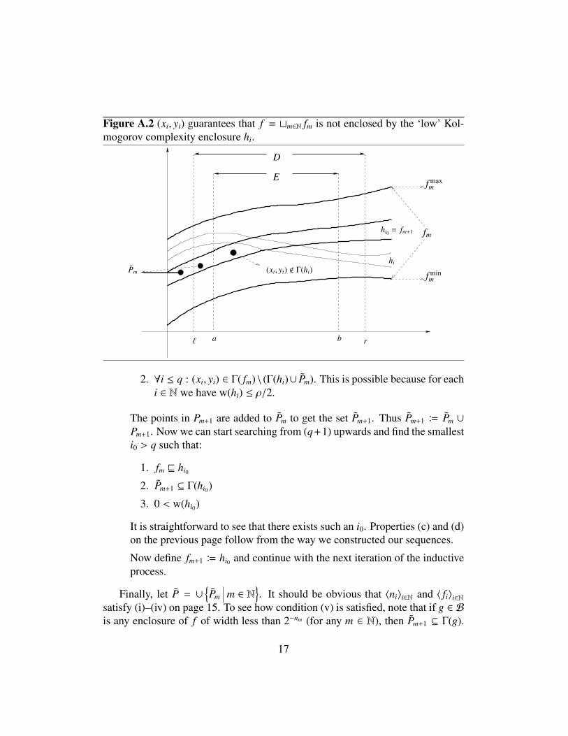
As Pm is a finite set, there exists a compact interval E = [a, b] of non-zerowidth (i. e. a < b) such that E ⊆ D \ π1(Pm), where π1 is the projection overthe first coordinate. In other words, E is a compact subinterval of D thatdoes not include the x-coordinate of any of the points in Pm.

Let Pm+1 = {(x0, y0), (x1, y1), . . . , (xq, yq)} ⊆ E × R be a set of points suchthat:

1. no two points have the same x-coordinate: ∀i < j ≤ q : xi , x j. Thisis possible because the compact interval E is not a singleton.

16

Figure A.2 (xi, yi) guarantees that f = tm∈N fm is not enclosed by the ‘low’ Kol-mogorov complexity enclosure hi.

D

E

fm

f maxm

f minm

hiPm

r` a b

= fm+1

(xi, yi) < Γ(hi)

hi0

2. ∀i ≤ q : (xi, yi) ∈ Γ( fm)\ (Γ(hi)∪ Pm). This is possible because for eachi ∈ N we have w(hi) ≤ ρ/2.

The points in Pm+1 are added to Pm to get the set Pm+1. Thus Pm+1 B Pm ∪

Pm+1. Now we can start searching from (q+1) upwards and find the smallesti0 > q such that:

1. fm v hi0

2. Pm+1 ⊆ Γ(hi0)

3. 0 < w(hi0)

It is straightforward to see that there exists such an i0. Properties (c) and (d)on the previous page follow from the way we constructed our sequences.

Now define fm+1 B hi0 and continue with the next iteration of the inductiveprocess.

Finally, let P = ∪{Pm m ∈ N

}. It should be obvious that 〈ni〉i∈N and 〈 fi〉i∈N

satisfy (i)–(iv) on page 15. To see how condition (v) is satisfied, note that if g ∈ Bis any enclosure of f of width less than 2−nm (for any m ∈ N), then Pm+1 ⊆ Γ(g).

17

This means that g cannot be any of the enclosures h0, h1, . . . , hq of Kolmogorovcomplexities less than θ(nm). �

Appendix B. Proof of Proposition 13

(a) Consider f , g ∈ K−1C (U) with optimal representations f and g, respectively.

Let us go through the proof for each of the arithmetic operators one by one:

addition: let h B f + g. To obtain a function enclosure hn of h of widthsmaller than 2−n, all we need is to take hn to be f (n + 1) + g(n + 1).Addition over finitely-representable approximations f (n+1) and g(n+1)adds only a constant C+ to the Kolmogorov complexity, in other words:

K(hn) ≤ K( f (n + 1)) + K(g(n + 1)) + C+

Remember that U is closed under addition and translation and it con-tains the constant function λn.C+. Thus KC(h) ∈ U.

subtraction: similar to the case of addition.

multiplication: let h B f × g. As g is continuous, it must be bounded bya constant Mg, i. e. ∀x ∈ [0, 1] : | g(x) | < Mg. Take Ng to be a naturalnumber such that 2Ng > Mg. To obtain a function enclosure hn of h ofwidth smaller than 2−n, all we need is to take hn to be f (n+Ng)×g(n+Ng).As × adds only a constant to the sum of the Kolmogorov complexitiesof f (n + Ng) and g(n + Ng), the rest of the proof for this case is similarto the case of addition.

division: similar to the case of multiplication: let h B f /g. Note that divisionby zero is ruled out. Hence, there exists a natural number Mg such that

∀x ∈ [0, 1] : | g(x) | >1

Mg

Thus, if we pick some Ng ∈ N large enough so that 2Ng > Mg, then∀n ≥ Ng : ∀x ∈ [0, 1] : (x, 0) < Γ(g(n)). In other words, for n greaterthan Ng, no enclosure g(n) crosses the x-axis. The rest of the proof issimilar to the case of multiplication.

(b) Let B = {θi i ∈ N} be a basis for U, which means that U = ∪ {↓θi i ∈ N}.We write cl(A) to denote the closure of a set A and we define:

UCL B ∪{cl(K−1

C (↓θi)) i ∈ N}

18

and prove thatK−1

C (U) = UCL

Obviously K−1C (U) ⊆ UCL. So, it will suffice to prove that:

∀i ∈ N : cl(K−1C (↓θi)) ⊆ K−1

C (U)

Fix a natural number p ∈ N and take an arbitrary function f ∈ cl(K−1C (↓ θp)).

This means that there exists a sequence 〈h0, h1, . . . , hn, . . .〉 of functions inK−1

C (↓θp) such that f = limi→∞ hi, where this limit is taken with regards to thesupremum norm. There exists a Cauchy subsequence

⟨hi0 , hi1 , . . . , hin , . . .

⟩of

this sequence which converges to f , therefore:

∀ j ∈ N : ‖ f − hi j‖sup< 2− j

Define the sequence 〈 f0, f1, . . . , fn, . . .〉 by letting f j B hi j for all j ∈ N. Eachfi has an optimal representation fi such that K( fi) ∈ ↓θp.

Now define the sequence of function enclosures 〈φ0, φ1, . . . , φn, . . .〉 by:

∀n ∈ N : φn = fn+1(n + 1) + λx.[−1

2n+2 ,1

2n+2 ] (B.1)

In other words, the nth enclosure φn is obtained by taking the enclosure fn+1(n+

1) (which has width smaller than 2−(n+1)) and adding the strip λx.[− 12n+2 ,

12n+2 ]

(which has the constant width 2−(n+1)). It is not difficult to see that the widthof φn is smaller than 2−n and f ∈ φn, because:

(a) fn+1(n + 1) approximates fn+1 to within 2−(n+1) accuracy;

(b) fn+1 in turn approximates f to within 2−(n+1) accuracy;

(c) φn contains a neighbourhood of fn+1 of width 2−(n+1)

Thus, 〈φ0, φ1, . . . , φn, . . .〉 is a valid binary representation of f . On the otherhand, the definition of φn as in (B.1) implies that:

∃C1,C2 ∈ N : K(φn) ≤ K( fn+1(n + 1)) + C1n + C2 (B.2)

The constant C2 is added to account for the addition and the lambda term,and C1 is needed because the length of the binary representation of 1/2n+2 islinearly proportional to n.

Remember that:

19

(i) ∀n ∈ N : fn ∈ ↓θp

(ii) U contains the linear function λn.C1n, the constant function λn.C2, andis closed under translation and addition.

Therefore, there exists a q ∈ N such that:

λn. θp(n) + C1n + C2 ∈↓θq

(by (B.2)) ⇒ λn.K(φn) ∈↓θq

(θq ∈ B) ⇒ λn.K(φn) ∈ U(U is a lower set) ⇒ KC( f ) ∈ U

⇒ f ∈ K−1C (U)

(c) Follows from (b).

(d) Let h = τ f + g and assume that h ∈ K−1C (U). But then by (a)

f = (h − g)/τ ∈ K−1C (U)

which is a contradiction. �

[1] Abramsky, S., Jung, A., 1994. Domain theory. In: Abramsky, S., Gabbay,D. M., Maibaum, T. S. E. (Eds.), Handbook of Logic in Computer Science.Vol. 3. Clarendon Press, Oxford, pp. 1–168.

[2] Barmpalias, G., Brodhead, P., Cenzer, D. A., Remmel, J. B., Weber, R.,2008. Algorithmic randomness of continuous functions. Archive for Mathe-matical Logic 46 (7–8), 533–546.

[3] Blum, L., Shub, M., Smale, S., 1989. On a theory of computation and com-plexity over the real numbers; NP completeness, recursive functions anduniversal machines. Bulletin of the American Mathematical Society (newseries) 21 (1), 1–46.

[4] Cai, J., Hartmanis, J., 1994. On Hausdorff and topological dimensions of theKolmogorov complexity of the real line. Journal of Computer and SystemSciences 49 (3), 605–619.

[5] Duracz, J. A., Konecny, M., August 2008. Polynomial func-tion enclosures and floating point software verification, in Pro-ceedings of CFV 2008 in Sydney, available from http://www-users.aston.ac.uk/˜konecnym/papers/cfv08.pdf.

20

[6] Edalat, A., Lieutier, A., 2002. Domain theory and differential calculus (func-tions of one variable). In: Proceedings of 17th Annual IEEE Symposium onLogic in Computer Science (LICS’02). Copenhagen, Denmark, pp. 277–286.

[7] Edalat, A., Sunderhauf, P., Jan. 1999. A domain theoretic approach to com-putability on the real line. Theoretical Computer Science 210, 73–98.

[8] Escardo, M. H., 1997. PCF extended with real numbers: a domain theo-retic approach to higher order exact real number computation. Ph.D. thesis,Imperial College.

[9] Farjudian, A., 2007. Shrad: A language for sequential real number compu-tation. Theory of Computing Systems 41 (1), 49–105.

[10] Farjudian, A., Konecny, M., 2008. Time complexity and convergence anal-ysis of domain theoretic Picard method. In: Hodges, W., de Queiroz, R.(Eds.), Proceedings of the 15th international workshop on Logic, Language,Information and Computation, WoLLIC ’08, Edinburgh, Scotland. Vol. 5110of Lecture Notes in Artificial Intelligence. Springer-Verlag, pp. 149–163.

[11] Fouche, W. L., 2000. Arithmetical representations of Brownian motion I.The Journal of Symbolic Logic 65 (1), 421–442.

[12] Fouche, W. L., 2008. Dynamics of a generic Brownian motion: Recursiveaspects. Theoretical Computer Science 394, 175–186.

[13] Gierz, G., Hofmann, K. H., Keimel, K., Lawson, J. D., Mislove, M. W.,Scott, D. S., 2003. Continuous Lattices and Domains. Vol. 93 of Encycloediaof Mathematics and its Applications. Cambridge University Press.

[14] Hunt, B. R., 1994. The prevalence of continuous nowhere differentiablefunctions. Proceedings of the American Mathematical Society 122 (3), 711–717.

[15] Hunt, B. R., Sauer, T., Yorke, J. A., October 1992. Prevalence: A translation-invariant “almost every” on infinite-dimensional spaces. Bulletin of theAmerican Mathematical Society 27 (2), 217–238.

[16] Lambov, B., 2007. Reallib: An efficient implementation of exact real arith-metic. Mathematical Structures in Computer Science 17 (1), 81–98.

21

[17] Montana, J. L., Pardo, L. M., 1998. On Kolmogorov complexity in the realTuring machine setting. Information Processing Letters 67, 81–86.

[18] Moore, R. E., 1966. Interval Analysis. Prentice-Hall, Englewood Cliffs, NewJersey, USA.

[19] Muller, N. T., 2001. The iRRAM: Exact arithmetic in C++. In: Selected Pa-pers from the 4th International Workshop on Computability and Complexityin Analysis (CCA). Vol. 2064. Springer-Verlag, pp. 222–252, lecture Notesin Computer Science.

[20] Neumaier, A., 2003. Taylor forms - use and limits. Reliable Computing 9 (1),43–79.

[21] Solomonoff, R., March 1964. A formal theory of inductive inference. Infor-mation and Control 7 (1), 1–22.

[22] Solomonoff, R., June 1964. A formal theory of inductive inference. Infor-mation and Control 7 (2), 224–254.

[23] Staiger, L., 2002. The Kolmogorov complexity of real numbers. TheoreticalComputer Science 284 (2), 455–466.

[24] Weihrauch, K., 2000. Computable Analysis, An Introduction. Springer-Verlag.

[25] Ziegler, M., Koolen, W. M., 2008. Kolmogorov complexity theory over thereals. Electronic Notes in Theoretical Computer Science 221, 153–169, pro-ceedings of the Fifth International Conference on Computability and Com-plexity in Analysis (CCA 2008).

22