On the Multivariate Extended Skew-Normal, Normal-exponential and Normal-gamma Distributions

by

CJ Adcock(1) and K Shutes(2)

(1) The University of Sheffield (2) Coventry University Business School

Abstract This paper presents expressions for the multivariate normal-exponential and normal-gamma distributions. It then presents properties of these distributions. These include conditional distributions and a new extension to Stein’s lemma. It is also shown that the multivariate normal-gamma and normal-exponential distribution are not in general closed under conditioning, although they are closed under linear transformations. The paper also demonstrates that there are relationships between the extended skew-normal distribution and the normal-gamma and normal-exponential distributions. Specifically, it is shown that certain limiting cases of the extended skew-normal distribution are normal-gamma and normal-exponential. One interpretation of these results is that the normal-exponential distribution may considered to be an alternative model to the extended skew-normal in some situations. An alternative point of view, however, is that the normal-exponential distribution is redundant since it may be replicated by a suitable extended skew-normal distribution. The theoretical results are supported by an empirical study of stock returns, which includes use of the multivariate distributions for portfolio selection. Keywords: exponential distribution, gamma distribution, moment generating function, multivariate extended skew-normal distribution, portfolio selection, Stein’s lemma. Correspondence Address: C J Adcock The Management School The University of Sheffield Mappin Street Sheffield, S1 4DT UK Email: c.j.adcock@shef.ac.uk Tel: +44 (0)114 222 3402

1

1. Introduction The skew-normal distribution which was introduced by Adelchi Azzalini, Azzalini (1985, 1986), is now almost certainly the best-known example of a general method of generating a skewed distribution. The method has various stochastic representations, there being a summary in Azzalini (2005). One method of generating the skew-normal distribution is to take the bivariate normal distribution of ( )YX, and then to consider the conditional distribution of X given that 0>Y . This representation is, with a change of notation, equivalent to considering the distribution of λVU + , where U has an arbitrary normal distribution and V , which is independent U , has the normal distribution ( )0,1N truncated from below at zero. A generalization in which V has the normal distribution ( ),1N τ truncated from below at zero is generally known as the extended skew-normal. The methods introduced by Azzalini and developed by him and many other authors have led to a wide range of distributions which possess rich theoretical properties. A different method of generating skewed distributions is to consider λVU + , where U has a symmetric distribution, but the non-negative variable V has a specified skewed distribution ab initio rather than being truncated. An example of this is the normal-exponential distribution, which was introduced by Aigner, Lovell and Schmidt (1977). As the name suggests, this specifies that U is normal and that V has an exponential distribution. An extension of this is the normal-gamma distribution which was introduced by Greene (1990) and which includes the normal-exponential as a special case. Although the theoretical foundations of skew-normal and related distributions are now both deep and mature, some authors express the view that applications are less well developed. The book by Genton (2004) rebuts this to some extent. Another exception to this is financial economics in which there has been a number of papers in recent years. This is particularly the case in portfolio theory where the multivariate skew-normal distribution has been used both for empirical studies and for the development of new theoretical results. Examples of the former may be found in Harvey et al (2010) and Adcock (2005). Examples of the latter are in Corns and Satchell (2007) and Adcock (2007), who presents an extension of Stein’s lemma (Stein, 1981) for the skew-normal distribution. A related but separate stream of work may be found in Simaan (1993). He proposes that the n-vector of returns on financial assets should be represented as Vλ+= UX . The n-vector U has a multivariate elliptically symmetric distribution and is independent of the non-negative scalar variable V , which has an unspecified skewed distribution. The n-vector λ , whose elements may take any real value, induces skewness in the return of individual assets. Multivariate versions of the normal-exponential and normal-gamma distributions are specific cases of the model proposed by Simaan, even though they do not appear explicitly in the literature. The aim of this paper is as follows. First, it is to present expressions for the multivariate normal-exponential and multivariate normal-gamma distributions. Secondly, it is present some properties of these distributions, specifically those which are of use in portfolio theory. These include conditional distributions, which are of relevance for asset pricing, and a new extension to Stein’s lemma which is relevant for portfolio selection. It is also shown that the multivariate normal-gamma and hence

2

multivariate normal-exponential distribution are not in general closed under conditioning, although they are closed under linear transformations. The paper also demonstrates that there are relationships between the extended skew-normal distribution and the normal-gamma and normal-exponential distributions. Specifically, it is shown that certain limiting cases of the extended skew-normal distribution are normal-gamma and normal-exponential. One interpretation of these results is that the normal-exponential distribution may considered to be an alternative model to the extended skew-normal in some situations. An alternative point of view, however, is that the normal-exponential distribution is redundant since it may be replicated by a suitable extended skew-normal distribution. The paper has five sections. Following a short summary of the multivariate extended skew-normal, henceforth MESN, distribution, the multivariate normal-exponential and normal-gamma distributions, henceforth MNE and MNG respectively, are derived in Section 2. Section 3 contains the main theoretical results of the paper. These describe conditions under which the normal-exponential distribution arises as a limiting case of the extended skew-normal distribution and some further properties of interest. Section 4 present background material for an empirical study of portfolio selection. This section contains the extension to Stein’s lemma for the MNG distribution. Section 5 reports an empirical study of the MESN and MNE distributions. Section 6 concludes. A short appendix contains the proofs of Lemmas reported in Sections 3 and 4. 2. Multivariate extended skew-normal normal-exponential and normal-gamma distributions The multivariate skew-normal distribution was introduced by Azzalini and Dalla Valle (1996). The multivariate extended skew-normal, MESN henceforth, distribution, which was first described in Adcock and Shutes (2001), may be obtained by considering the distribution of an n-vector Vλ+= UX . The vector U has a full rank multivariate normal distribution with mean vector μ and covariance matrix Σ . The elements of the vector λ may take any real values. The scalar variable V , which is distributed independently of U , has a normal distribution with mean τ and variance 1 truncated from below at zero. The distribution of X is denoted

( )τMESN n ,,, λμ Σ and the probability density function of the distribution is

( ) ( ) ( )τΦτΦτφfT

TT

n

+

−+++=

−

−

λλμλλλλμ

1

1

1

)(,;ΣxΣΣxx ,

where ( )xΦ is the standard normal distribution function evaluated at x . The notation

( )Σ,; μxnφ denotes the probability density function, evaluated at x , of a multivariate normal distribution with mean vector μ and covariance matrix Σ . The moment generating function (MGF) of the distribution, which is required below, is

{ } ( ) ( ).2)()(exp)( τΦτΦτM TTTT ++++= tλtλλtλμtt ΣX The vector of expected values and covariance matrix of X are, respectively

3

( ) { } ( ) { } ,τξvar, ΘΣXX =++==++= )(21)(ξτE T

1 λλδλμ τ where ( ) ,..2,1,)( =∂Φ∂= kxxlnx kk

kξ

The general notations δ and Θ are used

throughout the paper to denote the vector of expected returns and covariance matrix,

respectively. Omitting the subscript i, standardised values of skewness and kurtosis of

a typical element of X , which are required in Section 5, are

( ) ( ){ }[ ] ( ) ( ){ }[ ] σλψ,ψτξ11ψτξku',ψτξ11ψτξsk' 22

24

4232

23

3 =++=++= . A random vector X is said to have a multivariate normal-exponential, henceforth MNE, distribution if it is defined as above except that the variable V has an exponential distribution with scale equal, without loss of generality, to unity. The notation ( )λμ ,,ΣnMNE is used. The moment generating function (MGF) of the distribution, which is also required below, is

( ) ( ) 1.1/2exp)(M TTTT <−+= tλtλΣtttμt .,X

. The vector of expected values and covariance matrix of X under the MNE distribution are, respectively

( ) ( ) TE λλλμδ +==+== ΣΘXX var, . Under the multivariate normal-gamma distribution, henceforth MNG, the variable V has a gamma distribution with scale equal to one and υ degrees of freedom. That is, the probability density function of V is ( ) ( ) 0v0,υ,υΓevvf v1υ ≥>= −− . The MGF of this distribution is

( ) ( ) 1.1/2exp)(M TυTTT <−+= tλtλΣtttμt ,X The vector of expected values and covariance matrix of X under the MNE distribution are, respectively

( ) ( ) υυE Tλλλμδ +==+== ΣΘXX var, . The notation ( )υMNGn λ,μ ,,Σ is used. Since 1υ = is a special case, most of the results below are presented in terms of the MNG distribution, with corresponding results for the MNE distribution presented as corollaries. Standardised values of skewness and kurtosis for the MNG distribution are

( ) ( )2242323 υψ16υku',υψ12υsk' +=+= ψψ .

4

Univariate versions of the three distributions described in this section are referred to using the shorthand notations ESN, NE and NG respectively. Standard transformation of the variables gives the following results Lemma 1 - probability density function of the MNG distribution Let the n-vector X be distributed as ( )υ,MNGn λμ ,,Σ with at least one element of λ not equal to zero. The probability distribution of X has a density function given by:

( ) ( ) { }2Kf υ xxx T ~~2exp 12 −−= Σττ , where

( ) ( ) ( ) ( ) ( ) ( ) 2121nυυυ

-1T-1T2 ||2πωτΦτΔτΚ,1-ω τ,1/ω −−−==== ΣΣΣ-xx xλλλμ ~ ,~ , and ( ) ( ) ( )υΓYEΔ 1-υ

υ =τ where the random variable Y has the normal distribution ( ),1N τ truncated from below at zero.

For the MNE distribution, it is convenient to write the density function as follows. Corollary 1 Let the n-vector X be distributed as ( )λμ ,,ΣnMNE with at least one element of λ not equal to zero. The probability distribution of X has a density function given by:

( ) ( ){ } ( )τωωω Φ2-Kf T xλλxxλx TT ~~~2exp 1121122 −−−− −−= ΣΣΣΣ , where ( ) ( ) ( ) 2121n ||2πωτΦK −−−= Σ . Corollary 2 For 0≠λ the probability density function of the univariate form of the MNE distribution is

{ } { }[ ]λσλμ)(yδΦ2λσλμ)(yexpλf(y) λ

22-1 −−+−−= , where λδ equals 1 if 0λ > and –1 if 0λ < . The essence of the result in Corollary 2 is also reported in Dey and Liu(2007). Dey and Liu describe some of the properties of the univariate distribution, as does Shutes(2005). It is straightforward to verify that the equations above are indeed probability density functions. Both the multivariate and univariate density functions vanish at the tails and have a single mode. A standardized distribution may be obtained by defining a vector xAZ ~= and λΨ A= where A is the so-called square root matrix corresponding to the inverse of Σ .

5

The MNG distribution exhibits the following three useful properties. 1. Distribution of a sub-vector A sub-vector 1X of X is distributed as ( )υMNG 11n ,,, 11 λμ Σ , where 1μ and 1λ are the corresponding sub-vectors of μ and λ and 11Σ is the corresponding sub-matrix of Σ . 2. Closure under affine transformations Let the n-vector X be distributed as ( )υ,MNGn λμ ,,Σ and let b and A be respectively an n-vector and nm × matrix. The m-vector b+AX has the (possibly singular) distribution ( )υ,MNGn λμ AΑΣΑA ,, T . 3. Convolution Let the n-vectors iX be independently distributed as ( )υ,MNGn λμ ,,Σ for

k,1,i L= . The sum ∑=

k

1iiX is distributed as ( )kυ,kkMNGn λμ ,, Σ . The sample mean

vector X is distributed as ( )kυ,kkMNGn λμ ,,Σ . The following result is well known. It is reported here as it is used in the empirical study in Section 5. Lemma 2 – limiting normality of the MESN distribution Let X be distributed as ( )τMESN n ,,, λμ Σ . As −∞→τ the distribution of X tends to the multivariate normal ( )Σ,μnN . 3. Equivalence relations The results in this section first describe conditions under which the normal-exponential distribution arises as a limiting case of the extended skew-normal distribution and then presents two other properties of interest. Secondly, it is shown that under the same conditions the sum of extended skew-normal vectors is distributed as multivariate normal-gamma. The implications of these results are discussed in the conclusions in Section 6. The proofs of Lemmas 3, 5 and Lemmas 7 and 8 of Section 4 are in the appendix. Lemma 3 – a limiting MESN distribution Let ( )ττMESNn ,,,~ λμ −ΣX . As −∞→τ the distribution of X tends to the multivariate normal-exponential distribution ( )λμ ,,ΣnMNE . This lemma is one of the central results of the paper. It motivates the empirical study reported in Section 5. As described below, when the parameter τ is negative and of a

6

large magnitude, the two distributions can lead to very similar results, at least for the application described. Two other results are as follows and may be established using standard manipulations of the distribution. Lemma 4 facilitates use of the EM algorithm to estimate the parameters of the normal-gamma and normal-exponential distributions. It is also required for Lemma 5 which shows that the distribution is in general not closed under conditioning. Lemma 4 – conditional distribution of V given X Let the n-vector X be distributed as in Lemma 1. Conditional on xX = the distribution of the random variable ωVu = has a probability density function given by

( ) ( ) ( ) ( ){ } ( ){ }2τuexpuτΔυΓτΦuf 21υ1υ −−= −− .

Note that for the case 1υ = the conditional distribution is normal ( ),1N τ truncated from below at zero. To the best of out knowledge, this distribution does not appear explicitly in the literature. Its properties, which are not required for the current work and which have to be investigated using numerical methods, are a topic for further study. The following result is concerned with the conditional distribution of a sub-vector 1X given the values of a sub-vector 2X . Lemma 5 shows that that for the MNE distribution, the conditional distribution is in general multivariate extended skew-normal. Thus, the MNE distribution is not generally closed under conditioning. There is however a special case under which it is closed. Similar results for the conditional distributions under the MNG distribution are omitted. Lemma 5 – conditional distribution of 1X given 2X Let the n-vector X be distributed as ( )λμ ,,ΣMNE with at least one element of λ not equal to zero and let X be partitioned into two components 1X and 2X , with corresponding partitions for µ, λ and Σ. The following results hold: 1. When at least one element of 2λ is not equal to zero the conditional distribution

of 1X given 22 x=X is ( )2|12|12|12|1n τMESN1

,,, λμ Σ with

.),(

,,1)(

211

2212112|1221

221212|1

21

222

21

221212|1

21

222

21

222

ΣΣ Σ- ΣΣΣΣ

Σ

ΣΣ

Σ

Σ 2

−−

−

−

−

−

=−+=

−=

−−=

μxμμ

λλλλλ

λλμxλ

TT

T

2|1τ

2. When 2λ is the zero vector, the corresponding conditional distribution of 1X

given 22 x=X is ( )1,, λμ 2|12|1n1MNE Σ .

7

3. When 2

122121 λλ −− ΣΣ is the zero vector, the conditional distribution is

multivariate normal ( )2|12|1nN Σ,1μ .

Lemma 6 - convolution Let the n-vectors iX be independently distributed as ( )ττMESN n ,,, λμ −Σ for

k,1,i L= . As −∞→τ the distribution of ∑=

k

1iiX tends to ( )kυ,kkMNGn λμ ,, Σ and

the distribution of the sample mean vector X to ( )kυ,kkMNGn λμ ,,Σ . 4. Portfolio Selection Under the MESN and MNG Distributions To the best of our knowledge, the most common applications of the MESN distribution reported to date are in financial economics, specifically in portfolio selection and asset pricing. The MESN distribution was proposed as a parsimonious model for portfolio selection by Adcock and Shutes (2001). The attraction of the MESN model is that the asymmetry in asset returns, which is induced by the truncated variable denoted in previous sections by V , may be interpreted as a shock which represent a departure from financial market efficiency in the sense of Fama (1970). The effect of V on the returns of individual securities is described by the elements of the parameter vector λ , whose values may be positive, negative or zero. A similar and closely related line of research is described in Simaan(1993). In his work, Simaan proposes that the n-vector of asset returns may be represented as Vλ+= UX where the n-vector U has an elliptically symmetric distribution and the scalar V is a non-negative random variable, which is distributed independently of U . The three distributions described in this paper are all specific cases of the general model that Simaan proposes. Given the relationships that exist between the MNE and MNG distributions and certain limiting cases of the MESN distribution, it is natural to investigate the connections between the results of portfolio selection under these distributions. In general, portfolio selection is concerned with the return on a portfolio of assets. If asset returns are denoted by the n-vector X , portfolio return is the scalar variable

pT X=Xw where w is an n-vector of investment weights or proportions. The weights

usually (but not always) sum to unity. Formal portfolio selection chooses the investment proportions by maximising the expected utility of portfolio returns,

( ){ }pXUE where ( )U is a suitable utility function. Generally, this may be taken to mean that the first and second derivatives of ( )U are positive and negative respectively and that the expected values of ( )U , ( )U' and ( )'U' over the distribution used all exist. In practice the expected value of ( )U' is also allowed to be zero. When asset returns follow a multivariate normal distribution, it is well known that a consequence of Stein’s lemma, Stein (1981), is that the first order conditions for maximising expected utility take the form

( ) ( ) ( ){ } ( ){ } 0'',var ≥−== pp XUEXUEE θθ wXX ,

8

regardless of the investor’s utility function. It is this equation which generates Markowitz’ efficient frontier. In practice this is solved in the presence of inequality constraints on the weights using quadratic programming. In more recent work, Liu (1994) and Landsman and Nešlehová (2008) have shown that this result holds under all elliptically symmetric distributions. Adcock (2007) presents an extension for Stein’s lemma for the MESN distribution. For portfolio selection under MESN, the first order conditions are

( ) ( ) ( ) ( ) ( ){ } )(ξU'EU'E'U'E U'E 1N τ−+++ λwλλδ TΣ , where ( )E denotes expectation over the ( )τMESN n ,,, λμ Σ distribution and ( )nE denotes expectation over the multivariate normal distribution ( )Σ,N n μ . Since

( ) 0≥U' there is a non-negative preference for expected returns. The following lemma shows that there is also a non-negative preference for non-negative skewness. Lemma 7 – preference for skewness Let X ∼ MESN(µ, Σ, λ, τ) . The sign of ( ) ( )U'EU'EN − is the same as the sign of portfolio skewness λwT

p =λ . The first order conditions under the MESN distribution may be written in terms of the covariance matrix Θ as

( ) ( ) ( ) ( ){ } ( )[ ].T )(ξ'U'E)(ξU'EU'E'U'E U'E 21N ττ wΘw

λλδ −−++

In this case however, preference for skewness is not guaranteed to be non-negative. This reflects the fact that portfolio variance ww ΘT is smaller than the measure of risk implied by the first order conditions above which is ( )wλλw TT +Σ . An overall negative preference for skewness represents the price paid for the smaller risk measure. Nonetheless, the implication of the extension of Stein’s lemma for the MESN distribution is that the first order conditions for portfolio selection always take the form

0 , ≥+ θϕθ Θw -λδ . The scalar parameters θ , which is non-negative, and ϕ represent the investor’s preference for expected return and skewness. If these parameters are given, realistic portfolio selection may, as above, be performed using quadratic programming. For the MNG and MNE distributions, a similar investigation of portfolio selection requires the following extension to Stein’s lemma. A univariate version of the following result is a consequence of Theorem 2.1 of Kattumannil (2008). The setup for the lemma follows Liu (1994). An implication of this, details of which are omitted, is that there is also an extension to Siegel’s lemma (Siegel, 1993) which holds under the MNG and MNE distributions.

9

Lemma 8 - extension of Stein’s lemma for the MNG distribution Let X be an n-vector that has the distribution ( )υ,MNGn λμ ,,Σ . For any scalar valued function h(x) such that ix)/h( ∂∂ x is continuous almost everywhere and

∞<∂∂ ][ ))h(x/(E i X , i = 1, …, n, the following is true

( ){ } ( ){ } ( ){ } ( ){ }[ ]XXXΣXX hEhEhEh 1υ υυυ −+∇= +λ,cov , where ( ).υE denotes expectation taken over the ( )υ,MNGn λμ ,,Σ distribution. The n-vector ∇h(X) contains the elements ix)/h( ∂∂ x . Using Lemma 8, the first order conditions for portfolio selection under the MNG distribution may be written as

( ) ( ) ( ) ( ) ( )[ ] .λUEUEUE'U'E U'E Tpp1υυ λwλwδ =−−++ + ,'''' λυ υυΘ

It may be noted that standard stochastic dominance arguments imply that the quantity

( ) ( )'' UEUE 1 υυ −+ is non-positive. The sign of the term in the square brackets may depend on the utility function used. For example it is positive when the utility function takes the widely used form 0θ,e1 θx >− − and θλp −> . The first order conditions may be written in terms of the preference parameters θ and ϕ as

0 , >+ θϕθ Θw -λδ . The implication of this result is that under the MNG (and hence MNE) distribution, investors choose a portfolio which is located, according to their preferences, on a single mean-variance-skewness surface. A specific implication is that when the conditions of Lemma 3 hold the MESN and MNE efficient surfaces will be the same. 5. Examples And Empirical Study. This section of the paper compares the multivariate extended skew-normal and multivariate normal-exponential distributions. The aims are to demonstrate the implications of Lemma 3 and to investigate the differences between the skew-normal and normal-exponential distributions when the conditions of the lemma do not hold, but τ is less than zero. The section is in three parts. In the first, there are graphical and numerical comparisons of the two distributions. The second part of the section contains a short empirical study in which the parameters of the univariate extended skew-normal and normal-exponential distributions are estimated for the returns on stocks traded on the Czech stock market. The third part of this section reports an investigation into the use of the portfolio selection methods reported in Section 4. The aim of this sub-section is to investigate the extent of the differences between portfolios which are the result of using the two distributions.

10

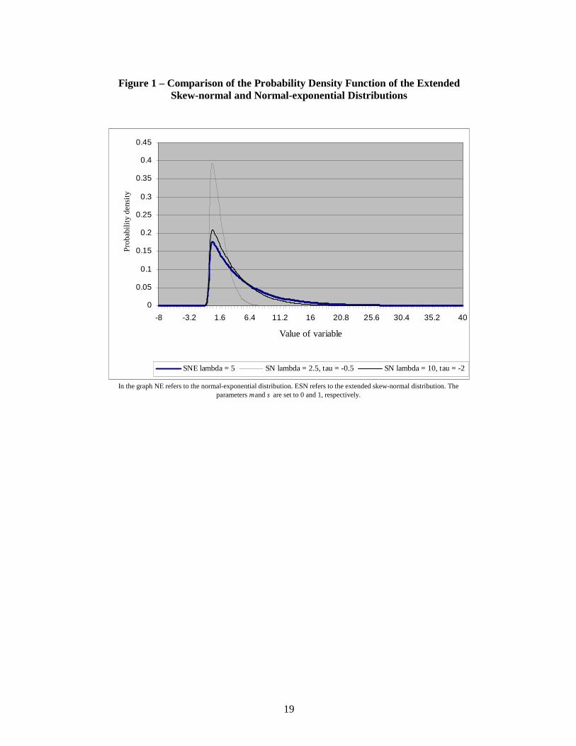
5.1 Graphical and numerical comparisons Figure 1 shows the probability density function of the normal-exponential distribution with parameters µ = 0, σ = 1 and λ = 5. According to Lemma 3, this distribution is the same as the limiting form of the extended skew-normal distribution

( )ττ ,50,1,ESN − as −∞→τ . Two examples of the extended skew-normal density function are shown. These correspond to values of τ set equal to –0.5 and –2.0 respectively. As the figure shows, the correspondence between the extended skew-normal distributions and the normal-exponential distribution is not close when τ = -0.5, but is when τ = -2.0. As τ decreases, the extended skew-normal density function increasingly resembles that of the corresponding normal-exponential distribution.

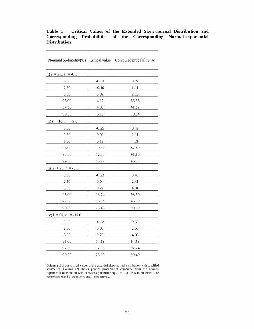
Figure 1 about here Table 1 shows critical values of the extended skew-normal distributions corresponding to a selection of specified nominal percent probabilities. These are set equal to 0.5, 2.5, 5.0, 95.0, 97.5 and 99.50. The critical values shown are exact for the four extended skew-normal distributions shown in the table. The table also shows the computed percent probabilities for the corresponding normal-exponential distribution. The table confirms the implications of the density plots in Figure 1. When τ = -0.5, the two densities are quite different. However, when τ = -2.0 and –5.0 the normal-exponential distribution is well approximated by the extended skew-normal distribution. When τ = -10.0 the difference in the computed probabilities are very small.

Table 1 about here

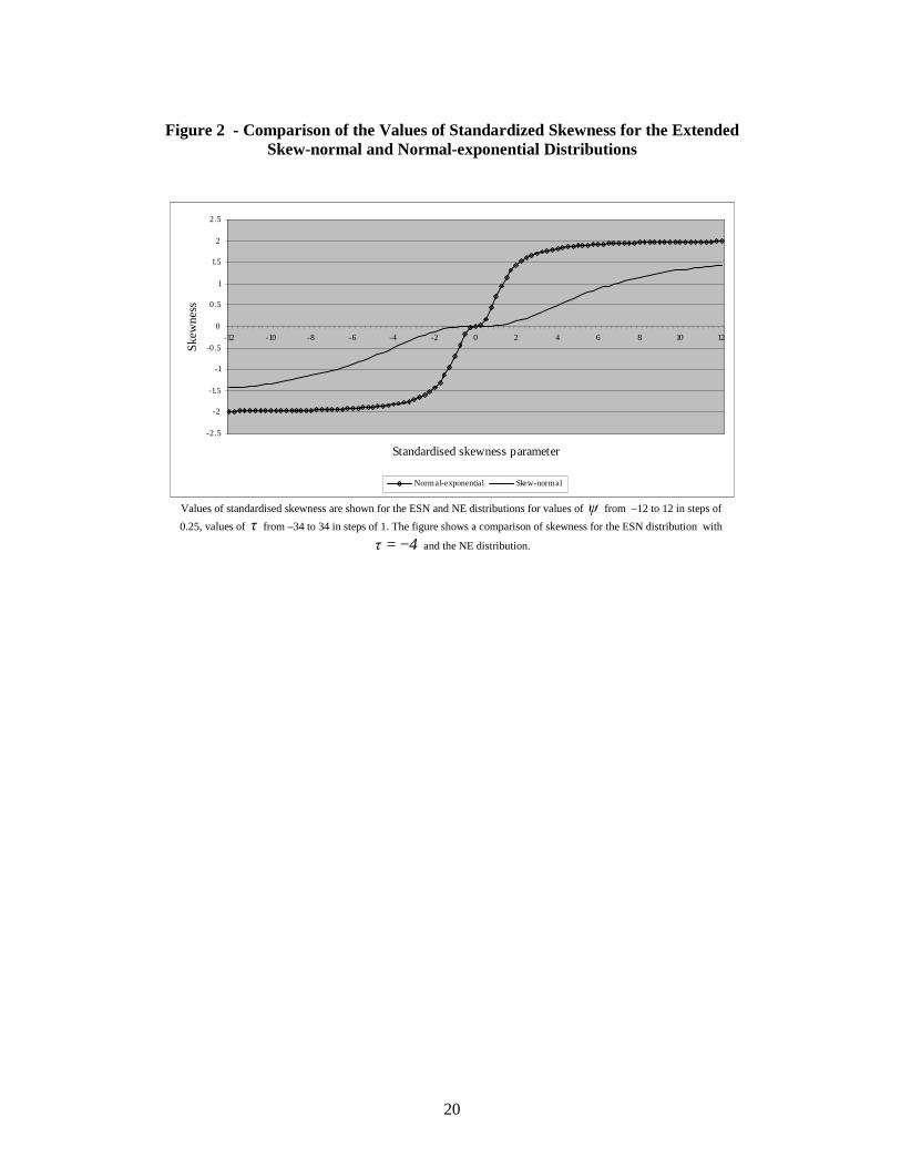
The implication of the graphs in Figure 1 and the computations in Table 1 is that it may be possible to use the normal-exponential distribution as an alternative to the extended skew-normal distribution in cases where the parameter τ is negative but does not necessarily have large magnitude. The example that follows in the second and third parts of this section illustrates this feature of the two models. It is also instructive to consider the behaviour of skewness and kurtosis under the two distributions. The formulae for the standardised values of these cumulants are reported in Section 2. The non-linear dependence of both skewness and kurtosis on the parameter τ for the ESN distribution rules out an analytical comparison. The following numerical comparison was therefore undertaken. Values of standardised skewness (kurtosis) were computed under the ESN and NE distributions for values of ψ from –12 to 12 in steps of 0.25, values of τ from –34 to 34 in steps of 1. The maximum value of skewness (kurtosis) occurs when 3τ −= (-4). Figures 2 and 3 show a comparison of skewness and kurtosis for the ESN distribution with 4τ −= and the NE distribution. The corresponding ESN values for 3−=τ are very similar and so are omitted.

11

.

Figures 2 & 3 about here The two figures demonstrate that both skewness and kurtosis are more sensitive to the value of ψ under the NE distribution. Under the NE distribution the maximum absolute value as ∞→ψ of standardised skewness is 2 and the maximum value of standardised kurtosis is 6. As Figures 2 and 3 demonstrate, the values of these two cumulants tend to these limits far more quickly under the NE distributions than under the ESN. Apart from the case 0ψ = the absolute values of standardised skewness and kurtosis are always less under the ESN distribution. This suggests that the NE distribution may be better at modelling both skewness and kurtosis than the ESN distribution. 5.2 Parameter estimation The example is based on daily closing prices of 14 of the constituent securities in the main stock market index in The Czech Republic. It uses data for 500 consecutive trading days, corresponding to about two calendar years. The period is from 4th June 2003 to 3rd May 2005. All data used is from Datastream and prices are measured in local currency. Price data are converted to returns in the standard way by computing logarithms. Stocks which did not have valid returns data for 500 days are excluded from the analysis. Returns on the index itself are included, giving a total of 15 securities. Univariate extended skew-normal and normal-exponential models were fitted separately to each stock. Model parameters were estimated by the method of maximum likelihood. The rationale for choosing an emerging stock market, such as The Czech Republic, is the following. One of the implications of standard theory in finance is that returns on stocks should have symmetric distributions. However, there is empirical evidence that suggests that the probability distributions of returns on some stocks do exhibit asymmetry in the form of skewness. In developed markets, such as the United States or the United Kingdom, skewness, when detected, is regarded by some as an anomaly, generally expected to be of relatively short-term duration. In emerging markets, by contrast, it may be regarded as an artefact of the process of emergence. The rapid growth of an emerging market coupled with structural changes in its modus operandi are suggested as two of the reasons why skewness may be observed in returns in stocks traded on its exchange. The papers by Badrinath and Chatterjee (1988), Beedles (1979), Chunhachinda et al (1997), Harvey and Siddique (1997), Kraus and Litzenberger (1976) and Samuelson (1970) provide a good introduction to the subject of skewness in asset returns and access to a more substantial list of references. Bekaert et al(1998) is concerned specifically with emerging markets.

Table 2 about here

12

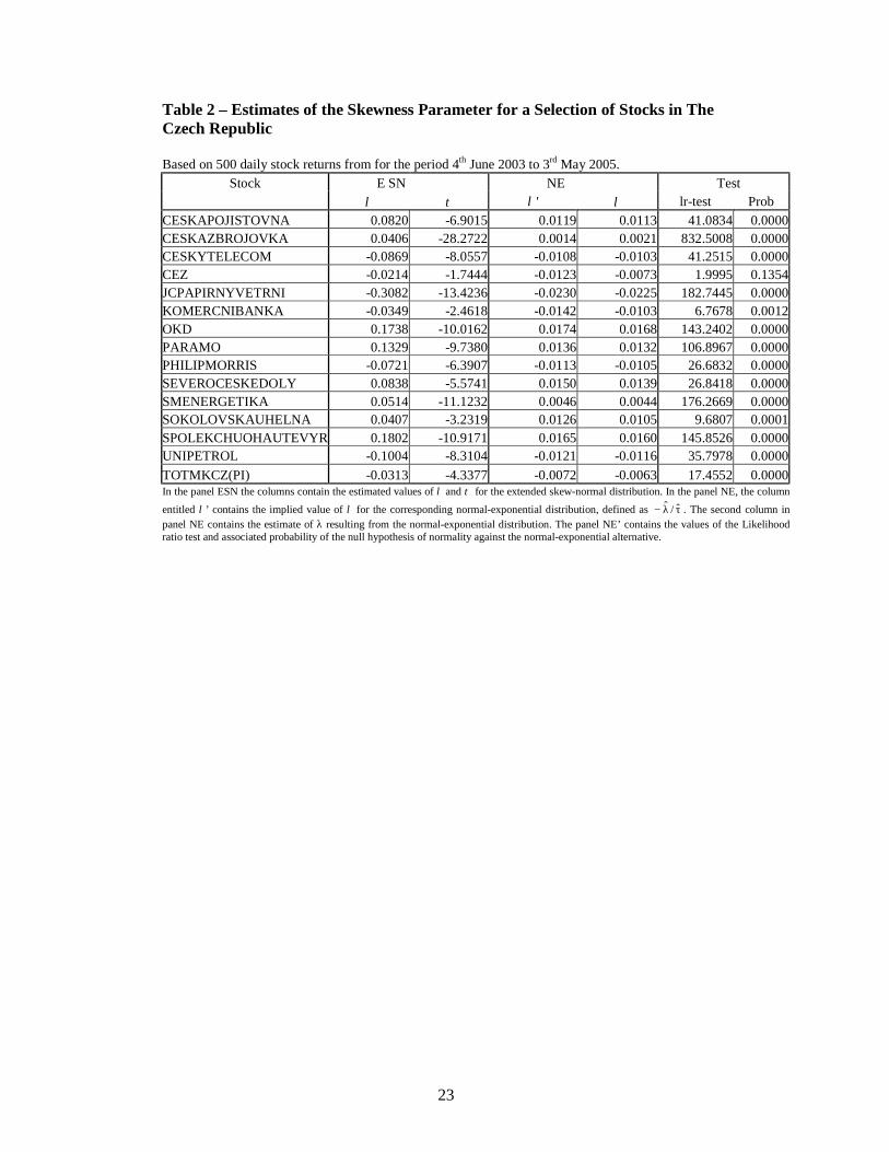
Panel ESN of Table 2 shows the estimates of λ and τ based on the extended skew-normal distribution for the 15 securities included in the study. The stocks, including the index, are identified by their Datastream name or mnemonic. The index is the last stock shown in the table. The first column of Panel NE, titled λ’, shows the implied value of lambda based on the estimated skew-normal parameters. Thus, for example, the implied value for the market index is -0.0313/4.3377 = -0.0072. From the panel NE, it will be clear that the estimated values of the skewness parameter lambda, titled λ, resulting from the normal-exponential distribution are generally similar to those implied by the parameters of the estimated extended skew-normal distribution. The second stock, CESKAZBROJOVKA, has an estimated value of τ equal to –28.3. This may be an example of the implications of Lemma 2; namely that this is a security where the skew-normal distribution has been employed when the normal distribution is in fact the correct model. Perusal of the table shows that the absolute differences between the direct estimate and the implied one are inversely proportional to tau. This provides some empirical support to the results in Table 1. The degree of agreement between the ESN and the NE distributions increases as tau decreases and that it is good for values of tau which are less than –3. It is well known that with the skew-normal distribution it is possible for maximum likelihood estimates of the skewness parameter to be on the boundary of the parameter space. The conditions for the likelihood ratio test do not therefore apply. For the normal-exponential distribution, there is no such restriction. As shown in the panel of Table 2 entitled ‘Test’, and for the time period studied, the null hypothesis that returns are normally distributed is rejected against the alternative that the distribution is normal-exponential at the 1% level of significance for 14 out of 15 Czech securities.

Table 3 about here

Table 3 shows computed critical values based on the estimated parameters for the two distributions. As the table shows, the critical values are generally in close agreement. The largest absolute discrepancy is 0.006. Out of the 120 entries in the table, corresponding to 15 securities and 8 levels of probability, only 6 exhibit an absolute discrepancy of 0.003 or greater. Table 4 shows comparison of the estimated values of µ and σ. Lemma 2 implies that they are the same for each model. The table of estimated values confirms that most are numerically similar.

Table 4 about here

To summarise: the material in this sub-section demonstrates cases when the extended skew-normal and normal-exponential distributions are similar. The short empirical study indicates that the latter distribution may be used in cases where τ is negative but not necessarily large in magnitude.

13

5.3 Portfolio selection For the portfolio selection study, the MESN and MNE distributions were fitted to the above data set. This resulted in estimates of the vectors, matrices and (for the MESN distribution) scalar that comprise the parameters of the two distributions. The aim of the exercise is to investigate the extent to which the two different distributions result in different portfolios. Under the MESN distribution, the estimated value of τ was –23.54. A likelihood ratio test of the null hypothesis of multivariate normality against the alternative multivariate normal-exponential distribution gave a p-value of less that 10-5. The efficient surface was constructed for a range of values of the risk appetite parameters θ and ϕ defined in Section 4. To reduce the volume of output, it was assumed that θ=ϕ . To make the exercise realistic, portfolio selection was performed subject to the common restrictions that all weights were non-negative and added to unity. Initial investigations showed that when 75.0=θ the portfolios consisted of a holding with a single weight of unity in the same asset. The value 0=θ generates the so-called minimum variance portfolio.

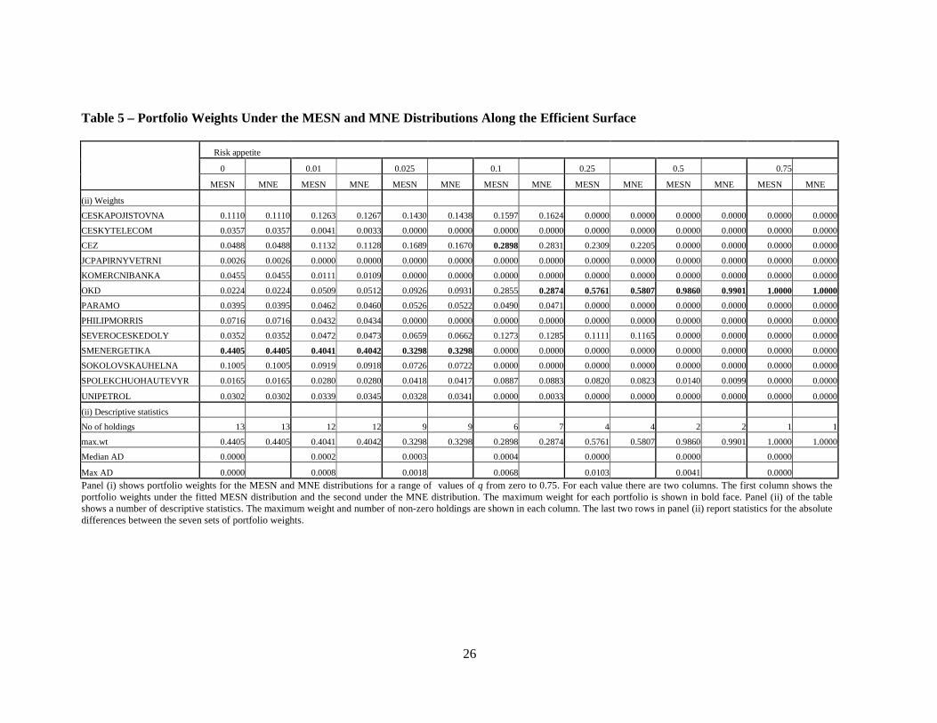
Table 5 about here Table 5 has two panels. Panel (i) shows portfolio weights computed for both the MESN and MNE distributions for a range of 7 values of θ from zero to 0.75, namely 0, 0.01, 0.025, 0.1, 0.25, 0.5 and 0.75. For each value of θ , there are two columns. The first column shows the portfolio weights under the fitted MESN distribution and the second the corresponding weights under the MNE distribution. For each portfolio the maximum weight is shown in bold face. Panel (ii) of the table shows a number of descriptive statistics. The maximum weight and number of (non-zero) holdings are shown in each column. These decrease progressively until, at risk appetite 0.75, there is a single holding in one security. The last two rows in panel (ii) report statistics for the absolute differences between the seven sets of portfolio weights. Thus, at risk 0.01, the maximum absolute difference in weights between the portfolios is 0.0008 or 0.08%. The median absolute difference is 0.02%.

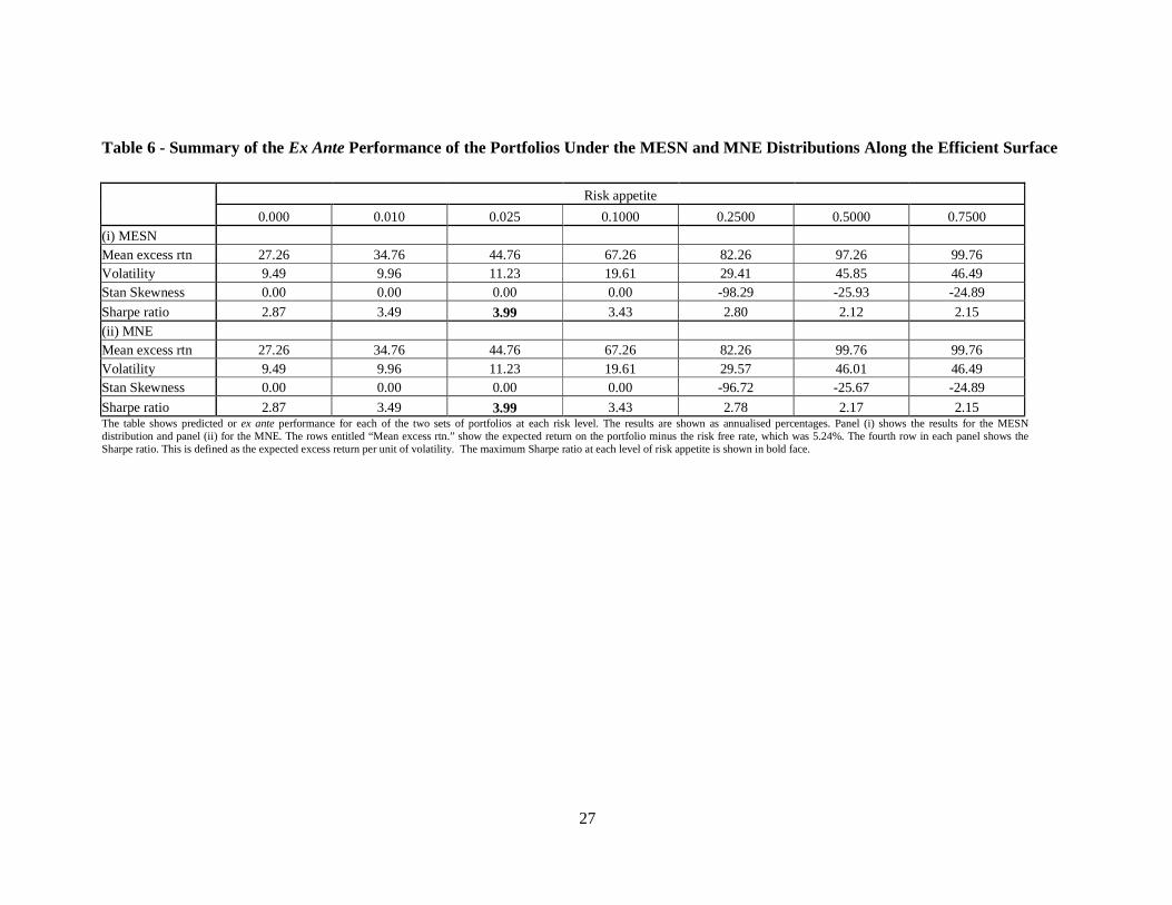
Table 6 about here Table 6 shows the predicted or ex ante performance for each of the two sets of portfolios at each risk level. As the original data was daily, the results are shown as annualised percentages. Panel (i) shows the results for the MESN distribution and panel (ii) for the MNE. The rows entitled “Mean excess rtn.” show the expected return on the portfolio minus the risk free rate. For the period under study, the annual risk free rate was 5.24%. The fourth row in each panel shows the Sharpe ratio. This is defined as the expected excess return per unit of volatility. This measure of portfolio performance is widely used in finance for both empirical and theoretical reasons. The maximum Sharpe ratio is shown in bold face.

14

Perusal of Table 5 leads to the following conclusions. Overall, the differences between the composition of the two portfolios at each level of risk are small. Furthermore, as risk increases both distributions lead to a single holding in the same asset. This reflects the fact that, not withstanding differences in the two fitted distributions, both lead to consistent estimators of the expected return and skewness which are the dominant terms in portfolio selection at high values of θ . Table 6 presents even stronger evidence about the similarity of the two portfolios. The ex ante performance statistics are almost identical. The main feature of note financially is that the maximum Sharpe ratio occurs at a low level of risk. It should be noted that Tables 5 and 6 are concerned with the results of the portfolio selection process under the two distributions. The realised or ex post performance of the portfolios is a topic for future study. The similarity of the weights in this study means that the performance of both portfolios will be very similar at all levels of risk. 6. Concluding remarks There is a body of empirical evidence, see for example Adcock(2004) or Shutes(2005) which suggests that applications of the skew-normal distribution in finance often give rise to estimated values of τ which are substantially less than zero. As long as 0τ ≠ , the skewness parameter vector may be reparameterised as τλ− . For the reasons described in Section 5 it is tempting to suggest that the normal-exponential distribution is a viable alternative model to the extended skew-normal. However, the general lack of closure of the MNE distribution under conditioning means that the MESN distribution offers superior theoretical facilities. Furthermore, the extended skew-normal distribution may always be estimated with the parameter τ set to any specified value. Indeed, Azzalini’s original model has 0τ = . This suggests that in practice the normal-exponential distribution may be replaced by the extended skew-normal, thus giving access if needed to the superior conditioning properties of the latter. By contrast, the MNG distribution is closed under convolution. This property is not exhibited by the MESN distribution. This property suggests that the multivariate normal-gamma model may offer superior opportunities for modelling asset returns and portfolio selection in situations where it is necessary to consider multiple time periods. This topic is also an issue that requires further study Lemmas 4 and 5 demonstrate some properties that connect the MESN and MNE distributions. Lemma 5 provides a framework for regression modelling under MNE errors. In general the regression of 1X on 2X is non-linear, but the lemma indicates there are special cases in which a linear model arises. The implication of this is that the use of a linear regression model may conceal non-normality in the unconditional distribution of the dependent variable. In financial applications, this may have an effect on portfolio selection because the skewness component may be omitted. A possible shortcoming of the MESN distribution is that the range of variation of standardized skewness and excess kurtosis is limited. By contrast, the possible range of variation under the MNE and MNG distributions is greater.

15

The examples and short empirical study in Sub-sections 5.1 and 5.2 demonstrate that the extended skew-normal and normal-exponential distributions give similar results for cases in which the parameter τ is negative but not necessarily very large in magnitude. For the portfolio selection study in Sub-section 5.3, in which the estimated value of the parameter τ is –24, the results from the two distributions are the same for all practical purposes. These results offer an empirical confirmation of the results of Lemma 3 Acknowledgements Thanks are due to a referee of an early version of this paper. He or she pointed out that the work would be enriched by the inclusion of a substantial application. The empirical study which is reported in Section 5 has led in turn to new theoretical insights, which are reported earlier in the paper. Appendix – proof of lemmas 2, 5, 7 and 8 Lemma 3 Using a standard result from Abramowitz and Stegun (1965, page 932), as

−∞→x the standard normal integral is

( ) |x|/xφΦ(x) ≈ . The moment generating function of X is { } ( ){ } ( ).-12)()-(exp)( τΦτττM TT2T2T tλtλλtλμtt Φ++= ΣX For 1<tλT

( ) ( ),1exp)( TTT tλtttμ −+=−∞→ 2tMlimτ /ΣX

which is the MGF of the MNE distribution. Lemma 5 First consider the case when 2λ is not a zero vector. From Lemma 3 and Corollary 1

of Lemma 1, the distribution of the variable UUT ~2

1222 =− λΣλ is, conditional on

22 x=X , normal ( ),1τN 2|1 truncated from below at zero. The conditional

distribution of 1X given 22 x=X and uU ~~ = is multivariate normal with mean vector

uu 2|12|1

21

22T2

21

2212122

122121

~~)( λμλλλλμxμ +=

−+−+

−

−−

Σ

ΣΣΣΣ ,

16

and conditional variance covariance matrix 211

2212112|1 ΣΣ Σ- ΣΣ −= . An Appeal to the definition of the multivariate extended skew-normal distribution in Section 2 or, equivalently, integration over the distribution of U~ given 22 x=X gives the result. For the case when 2λ is a zero vector, the distribution of U conditional on 22 x=X is exponential with scale 1. The conditional distribution of 1X given both 22 x=X and uU = is multivariate normal with mean vector u12|1 λμ + and covariance matrix

2|1Σ . Lemma 1 then gives the result. Part 3 follows at once. Lemma 7 The argument of U' is portfolio return XwX T

p = which has the univariate extended

skew-normal distribution ( )τ,λ,σ,μESN p2pp and which may be written as

UλYX pp += , where ( )2pp .σμN~Y and U is independently distributed as an

( )τ,1N variable truncated from below at zero. Thus

{ } ( ) ( ){ } ( ) ( ) ( )τΦdyduτ,1u,σ,μy,uλyU'yU']E[U'][U'E 0

12pp1pN ∫ ∫

∞ ∞

∞−

+−=− ϕϕ .

The inner integral is

( ) ( ) ( ) ( )∫∫∞

∞−

∞

∞−

+− dyσu,λμy,yU'dyσ,μy,yU' 2ppp1

2pp1 ϕϕ

Since the variable u is non-negative and 0U' ≥ this quantity depends on the sign of

λp . Using standard results in stochastic dominance theory implies that { } 0]E[U'][U'E N ≥− if 0λp ≥ .

Lemma 8 The proof of this lemma relies on the fact that the n-vector U and scalar V are independent and that

( ){ } ( ){ } ( ){ },,cov,cov,cov VhVVhh λλλ +++= UUUXX may be computed by integrating over the distributions of U and V in either order. The first term above requires only the use of Stein’s Lemma and gives ( ){ }.XΣ hEυ ∇ In the second term, the properties of the gamma distribution yield

( ) ( ){ } ( ){ } ( ){ }[ ].XXU hEhEVhυ-VE 1 υυυ −=+ +λ References

17

Abramowitz, M. and Stegun, I.(1965) Handbook of Mathematical Functions, New York: Dover.

Adcock, C. J. (2004). Capital Asset Pricing for UK Stocks Under the Multivariate Skew-Normal Distribution. In Genton, M. ed., Skew Elliptical Distributions and Their Applications: A Journey Beyond Normality. Chapman and Hall.

Adcock, C. J. (2005) Exploiting Skewness To Build An Optimal Hedge Fund With A Currency Overlay, The European Journal of Finance, 11, 445-462.

Adcock, C. J. (2007) Extensions of Stein’s Lemma for the Skew-normal Distribution, Communications in Statistics – Theory and Methods, 36, 1661-1672.

Adcock, C. J. and Shutes, K. (2001). Portfolio Selection Based on the Multivariate-Skew Normal Distribution, In Skulimowski, A. ed., Financial Modelling. Krakow: Progress & Business Publishers.

Aigner, D. J., Lovell C. K. and Schmidt, P. (1977). Formulation and Estimation of Stochastic Production Function Model. Journal of Econometrics, 12, 21-37.

Azzalini, A. (1985). A Class of Distributions Which Includes The Normal Ones. Scandinavian Journal of Statistics. 12, 171-178.

Azzalini, A. (1986). Further Results on a Class of Distributions Which Includes The Normal Ones, Statistica, 46, 199-208.

Azzalini, A. (2005). The skew-normal distribution and related multivariate families (with discussion by Marc G. Genton and a rejoinder by the author), Scandinavian Journal of Statistics., 32, 159–200.

Azzalini, A. and Dalla Valle, A. (1996). The Multivariate Skew-normal Distribution. Biometrika, 83, 715-726.

Badrinath S. G. and S. Chatterjee (1988) On Measuring Skewness and Elongation in Common Stock Return Distributions, Journal of Business, 61, p451-472.

Beedles, W. L. (1979) On The Asymmetry of Market Returns, Journal of Financial & Quantitative Analysis, 14, 653-660.

Bekaert G., C. R. Harvey, C. B. Erb and T. E. Viskantam (1998) Distributional Characteristics of Emerging Market Returns & Asset Allocation. Journal of Portfolio Management, 24, 102-116.

Chunhachinda, P., K. Dandapani, S. Hamid and A. J. Prakash (1997) Portfolio Selection and Skewness: Evidence From International Stock Markets. Journal of Banking and Finance, 21, 143-167.

Corns, T. R. A. and S. E. Satchell (2007) Skew Brownian Motion and Pricing European Options, The European Journal of Finance, 13, 523-544.

Dey, D. K. and Liu, J. (2004). Prior Elicitation From Expert Opinion: An Interactive Approach. Working Paper.

Fama, E. (1970) Efficient Capital Markets: A Review of Theory and Empirical Work, Journal of Finance, 25, 383-417.

Genton, M. (2004). Skew Elliptical Distributions and Their Applications: A Journey Beyond Normality, Boca Raton, Chapman and Hall.

Greene, W. H. (1990) A Gamma-distributed stochastic frontier model, Journal of Econometrics, 46, 141-163.

Harvey, C. R. and A. Siddique(1997) Conditional Skewness in Asset Pricing Tests, Journal of Finance, 55, 1263-1295.

Harvey, C. R., J. C. Leichty, M. W. Leichty and P. Muller (2010) Portfolio Selection With Higher Moments, Quantitative Finance, 10, 469 — 485

Kattumannil, S. K. (2009) On Stein’s identity and its applications, Statistics & Probability Letters, 79, 1444-1449.

18

Kraus, A. and R. H. Litzenberger(1976) Skewness Preference and The Valuation of Risk Assets, Journal of Finance, 31, 1085-1100.

Landsman, Z. & J. Nešlehová (2008) Stein’s Lemma for elliptical random vectors, Journal of Multivariate Analysis, 99, 912 – 927

Liu, J. S. (1994) Siegel’s Formula via Stein’s Identities, Statistics and Probability Letters, 21, 247-251.

Samuelson, P. A. (1970) The Fundamental Application Theorem of Portfolio Analysis in terms of Means, Variances and Higher Moments, Review of Economic Studies, 37, 537-542.

Shutes, K. (2005). Non-normality in Asset Pricing - Extensions and Applications of the Skew-Normal Distribution. PhD Thesis. University of Sheffield.

Siegel, A. F. (1993) A Surprising Covariance Involving the Minimum of Multivariate Normal Variables, Journal of the American Statistical Association, 88, 77-80.

Simaan, Y. (1993) Portfolio Selection and Asset Pricing- Three Parameter Framework. Management Science, 39, 568-587.

Stein, C. (1981) Estimation of the Mean of a Multivariate Normal Distribution, Annals of Statistics, 9, 1135-1151.

19

Figure 1 – Comparison of the Probability Density Function of the Extended

Skew-normal and Normal-exponential Distributions

0

0.05

0.1

0.15

0.2

0.25

0.3

0.35

0.4

0.45

-8 -3.2 1.6 6.4 11.2 16 20.8 25.6 30.4 35.2 40

Value of variable

Prob

abili

ty d

ensi

ty

SNE lambda = 5 SN lambda = 2.5, tau = -0.5 SN lambda = 10, tau = -2

In the graph NE refers to the normal-exponential distribution. ESN refers to the extended skew-normal distribution. The parameters µ and σ are set to 0 and 1, respectively.

20

Figure 2 - Comparison of the Values of Standardized Skewness for the Extended

Skew-normal and Normal-exponential Distributions

-2 .5

-2

-1.5

-1

-0 .5

0

0 .5

1

1.5

2

2 .5

-12 -10 -8 -6 -4 -2 0 2 4 6 8 10 12

Standardised skewness parameter

Skew

ness

Normal-exponential Skew-normal

Values of standardised skewness are shown for the ESN and NE distributions for values of ψ from –12 to 12 in steps of 0.25, values of τ from –34 to 34 in steps of 1. The figure shows a comparison of skewness for the ESN distribution with

4τ −= and the NE distribution.

21

Figure 3 - Comparison of the Values of Standardized Kurtosis for the Extended Skew-normal and Normal-exponential Distributions

0

1

2

3

4

5

6

7

-12 -10 -8 -6 -4 -2 0 2 4 6 8 10 12

Standardised skewness parameter

Kur

tosi

s

Normal-exponential Skew-normal

Values of standardised kurtosis are shown for the ESN and NE distributions for values of ψ from –12 to 12 in steps of 0.25, values of τ from –34 to 34 in steps of 1. The figure shows a comparison of kurtosis for the ESN distribution with

4τ −= and the NE distribution.

22

Table 1 – Critical Values of the Extended Skew-normal Distribution and Corresponding Probabilities of the Corresponding Normal-exponential Distribution

Nominal probability(%) Critical value Computed probability(%)

(i) λ = 2.5, τ = -0.5

0.50 -0.33 0.22

2.50 -0.10 1.11

5.00 0.02 2.19

95.00 4.17 56.55

97.50 4.83 61.92

99.50 6.18 70.94

(ii) λ = 10, τ = -2.0

0.50 -0.25 0.42

2.50 0.02 2.11

5.00 0.18 4.21

95.00 10.52 87.80

97.50 12.55 91.86

99.50 16.87 96.57

(iii) λ = 25, τ = -5.0

0.50 -0.23 0.49

2.50 0.04 2.41

5.00 0.22 4.81

95.00 13.74 93.59

97.50 16.74 96.48

99.50 23.48 99.09

(iv) λ = 50, τ = -10.0

0.50 -0.22 0.50

2.50 0.05 2.50

5.00 0.23 4.93

95.00 14.63 94.63

97.50 17.95 97.24

99.50 25.60 99.40

Column (1) shows critical values of the extended skew-normal distribution with specified parameters. Column (2) shows percent probabilities computed from the normal-exponential distribution with skewness parameter equal to -λ/τ, ie 5 in all cases. The parameters µ and σ are set to 0 and 1, respectively.

23

Table 2 – Estimates of the Skewness Parameter for a Selection of Stocks in The Czech Republic Based on 500 daily stock returns from for the period 4th June 2003 to 3rd May 2005.

Stock E SN NE Test λ τ λ' λ lr-test Prob CESKAPOJISTOVNA 0.0820 -6.9015 0.0119 0.0113 41.0834 0.0000CESKAZBROJOVKA 0.0406 -28.2722 0.0014 0.0021 832.5008 0.0000CESKYTELECOM -0.0869 -8.0557 -0.0108 -0.0103 41.2515 0.0000CEZ -0.0214 -1.7444 -0.0123 -0.0073 1.9995 0.1354JCPAPIRNYVETRNI -0.3082 -13.4236 -0.0230 -0.0225 182.7445 0.0000KOMERCNIBANKA -0.0349 -2.4618 -0.0142 -0.0103 6.7678 0.0012OKD 0.1738 -10.0162 0.0174 0.0168 143.2402 0.0000PARAMO 0.1329 -9.7380 0.0136 0.0132 106.8967 0.0000PHILIPMORRIS -0.0721 -6.3907 -0.0113 -0.0105 26.6832 0.0000SEVEROCESKEDOLY 0.0838 -5.5741 0.0150 0.0139 26.8418 0.0000SMENERGETIKA 0.0514 -11.1232 0.0046 0.0044 176.2669 0.0000SOKOLOVSKAUHELNA 0.0407 -3.2319 0.0126 0.0105 9.6807 0.0001SPOLEKCHUOHAUTEVYR 0.1802 -10.9171 0.0165 0.0160 145.8526 0.0000UNIPETROL -0.1004 -8.3104 -0.0121 -0.0116 35.7978 0.0000TOTMKCZ(PI) -0.0313 -4.3377 -0.0072 -0.0063 17.4552 0.0000In the panel ESN the columns contain the estimated values of λ and τ for the extended skew-normal distribution. In the panel NE, the column entitled λ’ contains the implied value of λ for the corresponding normal-exponential distribution, defined as τλ− ˆ/ˆ . The second column in panel NE contains the estimate of λ resulting from the normal-exponential distribution. The panel NE’ contains the values of the Likelihood ratio test and associated probability of the null hypothesis of normality against the normal-exponential alternative.

24

Table 3 – Comparison of Estimated Critical Values for a Selection of Czech Stocks Based on the Extended Skew-normal and Normal-exponential Distributions Based on 500 daily stock returns from for the period 4th June 2003 to 3rd May 2005. Nominal probability (%) Nominal probability (%)

0.050 0.500 2.500 5.000 95.000 97.500 99.500 99.950 0.050 0.500 2.500 5.000 95.000 97.500 99.500 99.950

(i) ESN (ii) NE

CESKAPOJISTOVNA -0.0450 -0.0350 -0.0270 -0.0230 0.0310 0.0390 0.0560 0.0810 -0.0450 -0.0360 -0.0270 -0.0230 0.0310 0.0390 0.0570 0.0830

CESKAZBROJOVKA -0.0020 -0.0020 -0.0010 -0.0010 0.0040 0.0040 0.0070 0.0100 -0.0030 -0.0020 -0.0020 -0.0020 0.0050 0.0070 0.0100 0.0150

CESKYTELECOM -0.0760 -0.0540 -0.0370 -0.0300 0.0280 0.0330 0.0420 0.0530 -0.0780 -0.0540 -0.0380 -0.0300 0.0270 0.0320 0.0420 0.0520

CEZ -0.0600 -0.0450 -0.0320 -0.0260 0.0300 0.0350 0.0450 0.0570 -0.0630 -0.0460 -0.0330 -0.0270 0.0290 0.0340 0.0440 0.0560

JCPAPIRNYVETRNI -0.1620 -0.1110 -0.0750 -0.0590 0.0510 0.0600 0.0770 0.0960 -0.1630 -0.1110 -0.0750 -0.0590 0.0510 0.0600 0.0770 0.0960

KOMERCNIBANKA -0.0730 -0.0530 -0.0380 -0.0300 0.0290 0.0340 0.0440 0.0550 -0.0790 -0.0550 -0.0380 -0.0310 0.0290 0.0340 0.0440 0.0550

OKD -0.0550 -0.0440 -0.0340 -0.0280 0.0440 0.0560 0.0830 0.1200 -0.0550 -0.0440 -0.0340 -0.0280 0.0440 0.0550 0.0830 0.1210

PARAMO -0.0490 -0.0390 -0.0300 -0.0260 0.0360 0.0450 0.0660 0.0950 -0.0490 -0.0390 -0.0300 -0.0260 0.0350 0.0440 0.0650 0.0960

PHILIPMORRIS -0.0760 -0.0530 -0.0370 -0.0290 0.0270 0.0310 0.0400 0.0510 -0.0780 -0.0540 -0.0370 -0.0300 0.0260 0.0310 0.0400 0.0500

SEVEROCESKEDOLY -0.0630 -0.0490 -0.0380 -0.0320 0.0410 0.0510 0.0720 0.1010 -0.0630 -0.0500 -0.0380 -0.0320 0.0410 0.0500 0.0730 0.1050

SMENERGETIKA -0.0170 -0.0130 -0.0100 -0.0090 0.0120 0.0150 0.0220 0.0320 -0.0170 -0.0130 -0.0100 -0.0090 0.0110 0.0140 0.0220 0.0320

SOKOLOVSKAUHELNA -0.0540 -0.0430 -0.0330 -0.0280 0.0320 0.0400 0.0550 0.0750 -0.0540 -0.0430 -0.0330 -0.0280 0.0320 0.0400 0.0570 0.0810

SPOLEKCHUOHAUTEVYR -0.0590 -0.0470 -0.0360 -0.0300 0.0420 0.0540 0.0790 0.1150 -0.0590 -0.0470 -0.0360 -0.0310 0.0420 0.0530 0.0790 0.1160

UNIPETROL -0.0870 -0.0610 -0.0430 -0.0340 0.0350 0.0410 0.0530 0.0660 -0.0890 -0.0620 -0.0430 -0.0350 0.0350 0.0410 0.0520 0.0660

TOTMKCZ(PI) -0.0430 -0.0300 -0.0210 -0.0160 0.0170 0.0200 0.0250 0.0310 -0.0460 -0.0310 -0.0210 -0.0170 0.0160 0.0190 0.0240 0.0300 The table shows computed critical values based on the estimated parameters for the two distributions. Panel (i) is the ESN and panel (ii) the NE. The largest absolute discrepancy is between the two distributions 0.006. Out of the 120 entries in the table, corresponding to 15 securities and 8 levels of probability, only 6 exhibit an absolute discrepancy of 0.003 or greater.

25

Table 4 – Estimates of the Location and Scale Parameters for a Selection of Stocks in The Czech Republic Based on 500 daily stock returns from for the period 4th June 2003 to 3rd May 2005.

A B Stock location (µ) scale (σ) ESN NE EXN NE CESKAPOJISTOVNA -0.0093 -0.0092 0.0123 0.0123 CESKAZBROJOVKA -0.0006 -0.0008 0.0005 0.0005 CESKYTELECOM 0.0109 0.0108 0.0144 0.0144 CEZ 0.0112 0.0097 0.0153 0.0155 JCPAPIRNYVETRNI 0.0232 0.0231 0.0256 0.0255 KOMERCNIBANKA 0.0122 0.0111 0.0149 0.0151 OKD -0.0127 -0.0126 0.0149 0.0149 PARAMO -0.0109 -0.0108 0.0134 0.0132 PHILIPMORRIS 0.0112 0.0110 0.0136 0.0137 SEVEROCESKEDOLY -0.0117 -0.0114 0.0177 0.0176 SMENERGETIKA -0.0036 -0.0035 0.0046 0.0044 SOKOLOVSKAUHELNA -0.0098 -0.0094 0.0152 0.0151 SPOLEKCHUOHAUTEVYR -0.0135 -0.0134 0.0158 0.0158 UNIPETROL 0.0138 0.0136 0.0179 0.0178 TOTMKCZ(PI) 0.0079 0.0077 0.0079 0.0080 The two columns of panel A show the estimated values of the location parameter µ arising from the extended skew-normal(ESN) model and normal-exponential (NE) model respectively. Panel B shows comparable information for the scale parameter σ.

26

Table 5 – Portfolio Weights Under the MESN and MNE Distributions Along the Efficient Surface Risk appetite

0 0.01 0.025 0.1 0.25 0.5 0.75

MESN MNE MESN MNE MESN MNE MESN MNE MESN MNE MESN MNE MESN MNE

(ii) Weights

CESKAPOJISTOVNA 0.1110 0.1110 0.1263 0.1267 0.1430 0.1438 0.1597 0.1624 0.0000 0.0000 0.0000 0.0000 0.0000 0.0000

CESKYTELECOM 0.0357 0.0357 0.0041 0.0033 0.0000 0.0000 0.0000 0.0000 0.0000 0.0000 0.0000 0.0000 0.0000 0.0000

CEZ 0.0488 0.0488 0.1132 0.1128 0.1689 0.1670 0.2898 0.2831 0.2309 0.2205 0.0000 0.0000 0.0000 0.0000

JCPAPIRNYVETRNI 0.0026 0.0026 0.0000 0.0000 0.0000 0.0000 0.0000 0.0000 0.0000 0.0000 0.0000 0.0000 0.0000 0.0000

KOMERCNIBANKA 0.0455 0.0455 0.0111 0.0109 0.0000 0.0000 0.0000 0.0000 0.0000 0.0000 0.0000 0.0000 0.0000 0.0000

OKD 0.0224 0.0224 0.0509 0.0512 0.0926 0.0931 0.2855 0.2874 0.5761 0.5807 0.9860 0.9901 1.0000 1.0000 PARAMO 0.0395 0.0395 0.0462 0.0460 0.0526 0.0522 0.0490 0.0471 0.0000 0.0000 0.0000 0.0000 0.0000 0.0000

PHILIPMORRIS 0.0716 0.0716 0.0432 0.0434 0.0000 0.0000 0.0000 0.0000 0.0000 0.0000 0.0000 0.0000 0.0000 0.0000

SEVEROCESKEDOLY 0.0352 0.0352 0.0472 0.0473 0.0659 0.0662 0.1273 0.1285 0.1111 0.1165 0.0000 0.0000 0.0000 0.0000

SMENERGETIKA 0.4405 0.4405 0.4041 0.4042 0.3298 0.3298 0.0000 0.0000 0.0000 0.0000 0.0000 0.0000 0.0000 0.0000

SOKOLOVSKAUHELNA 0.1005 0.1005 0.0919 0.0918 0.0726 0.0722 0.0000 0.0000 0.0000 0.0000 0.0000 0.0000 0.0000 0.0000

SPOLEKCHUOHAUTEVYR 0.0165 0.0165 0.0280 0.0280 0.0418 0.0417 0.0887 0.0883 0.0820 0.0823 0.0140 0.0099 0.0000 0.0000

UNIPETROL 0.0302 0.0302 0.0339 0.0345 0.0328 0.0341 0.0000 0.0033 0.0000 0.0000 0.0000 0.0000 0.0000 0.0000

(ii) Descriptive statistics

No of holdings 13 13 12 12 9 9 6 7 4 4 2 2 1 1

max.wt 0.4405 0.4405 0.4041 0.4042 0.3298 0.3298 0.2898 0.2874 0.5761 0.5807 0.9860 0.9901 1.0000 1.0000

Median AD 0.0000 0.0002 0.0003 0.0004 0.0000 0.0000 0.0000

Max AD 0.0000 0.0008 0.0018 0.0068 0.0103 0.0041 0.0000 Panel (i) shows portfolio weights for the MESN and MNE distributions for a range of values of θ from zero to 0.75. For each value there are two columns. The first column shows the portfolio weights under the fitted MESN distribution and the second under the MNE distribution. The maximum weight for each portfolio is shown in bold face. Panel (ii) of the table shows a number of descriptive statistics. The maximum weight and number of non-zero holdings are shown in each column. The last two rows in panel (ii) report statistics for the absolute differences between the seven sets of portfolio weights.

27

Table 6 - Summary of the Ex Ante Performance of the Portfolios Under the MESN and MNE Distributions Along the Efficient Surface

Risk appetite 0.000 0.010 0.025 0.1000 0.2500 0.5000 0.7500 (i) MESN Mean excess rtn 27.26 34.76 44.76 67.26 82.26 97.26 99.76 Volatility 9.49 9.96 11.23 19.61 29.41 45.85 46.49 Stan Skewness 0.00 0.00 0.00 0.00 -98.29 -25.93 -24.89 Sharpe ratio 2.87 3.49 3.99 3.43 2.80 2.12 2.15 (ii) MNE Mean excess rtn 27.26 34.76 44.76 67.26 82.26 99.76 99.76 Volatility 9.49 9.96 11.23 19.61 29.57 46.01 46.49 Stan Skewness 0.00 0.00 0.00 0.00 -96.72 -25.67 -24.89 Sharpe ratio 2.87 3.49 3.99 3.43 2.78 2.17 2.15 The table shows predicted or ex ante performance for each of the two sets of portfolios at each risk level. The results are shown as annualised percentages. Panel (i) shows the results for the MESN distribution and panel (ii) for the MNE. The rows entitled “Mean excess rtn.” show the expected return on the portfolio minus the risk free rate, which was 5.24%. The fourth row in each panel shows the Sharpe ratio. This is defined as the expected excess return per unit of volatility. The maximum Sharpe ratio at each level of risk appetite is shown in bold face.