On the Political Economy of Labor Market Flexibility · Gilles Saint-Paul CERAS AND DELTA, PARIS,...

This PDF is a selection from an out-of-print volume from the NationalBureau of Economic Research

Volume Title: NBER Macroeconomics Annual 1993, Volume 8

Volume Author/Editor: Olivier Blanchard and Stanley Fischer, editors

Volume Publisher: MIT Press

Volume ISBN: 0-252-02364-4

Volume URL: http://www.nber.org/books/blan93-1

Conference Date: March 12-13, 1993

Publication Date: January 1993

Chapter Title: On the Political Economy of Labor Market Flexibility

Chapter Author: Gilles Saint-Paul

Chapter URL: http://www.nber.org/chapters/c11000

Chapter pages in book: (p. 151 - 196)

Gilles Saint-Paul CERAS AND DELTA, PARIS, AND CEPR

On the Political Economy of Labor

Market Flexibility*

1. Introduction

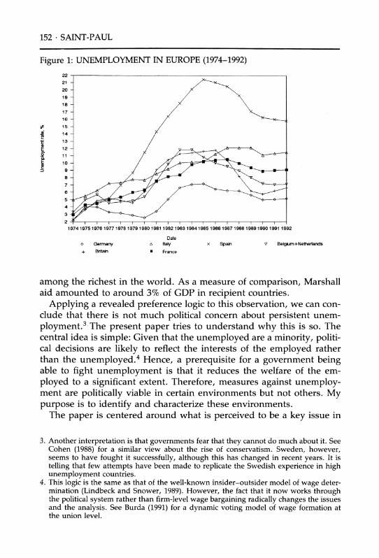
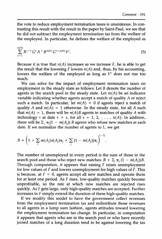
Figure 1 plots the rise in unemployment in Europe since 1974. The major fact is that European unemployment has been very high for the last 12

years, say 8-10%, and has no marked tendency to go down.1 The economic costs of this are very large-the same order of magni-

tude, as a share in GDP, as the unemployment rate itself.2 It is not unreasonable to think that in a country like France or Italy, some 5% of GDP have been lost every year for 12 consequent years as a result of high unemployment. These losses are similar in magnitude to those created by the major destruction in capital stock associated with a war.

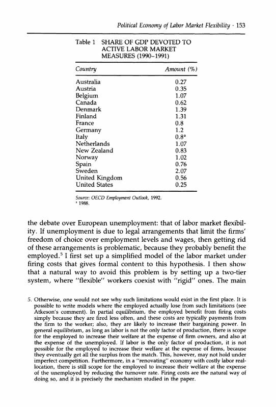
In the face of it, what have governments done? Table 1 reports the share of GDP devoted to active labor market measures, i.e., excluding unemployment benefits. With the notable exception of Sweden, the

figures stand around a modest 1% of GDP-this in countries that are

*DELTA is a joint research unit ENS-EHESS-CNRS. This paper was prepared for the NBER Annual Conference on Macroeconomics, Cambridge, USA, March 12-13, 1993. The author is grateful to Alberto Alesina, Samuel Bentolila, Fischer Black, Olivier Blanchard, Pascal Marianna, and my discussants Andy Atkeson and Bob Solow, as well as seminar participants at New York University and Northwestern University for helpful comments and suggestions. 1. Considerable empirical and theoretical research has of course been devoted to the

European Unemployment problem. The reader can refer to Bean (1993) or Layard et al. (1990).

2. Given that this is a long-run phenomenon, we want to use a neo-classical production function while allowing capital to vary. Under constant returns, the yearly output loss is therefore of the order of magnitude of the unemployment rate itself, although one would want to correct for manpower's quality and labor supply elasticity. Okun's law is inappropriate here, because it only makes sense for short-run cyclical variations in employment.

152 SAINT-PAUL

Figure 1: UNEMPLOYMENT IN EUROPE (1974-1992)

22

21-

20

19

17

16

15

14

13

12-

11

10 9

7

6

5

4

3

1974 19751976 1977 1978 1979 1980 1981 1982 1983 19841985 1986 1987 1988 19891990 1991 1992

Date o Germany A Italy x Spain v Belgium+Netherlands

+ Brtain * France

among the richest in the world. As a measure of comparison, Marshall aid amounted to around 3% of GDP in recipient countries.

Applying a revealed preference logic to this observation, we can conclude that there is not much political concern about persistent unemployment.3 The present paper tries to understand why this is so. The central idea is simple: Given that the unemployed are a minority, political decisions are likely to reflect the interests of the employed rather than the unemployed.4 Hence, a prerequisite for a government being able to fight unemployment is that it reduces the welfare of the employed to a significant extent. Therefore, measures against unemployment are politically viable in certain environments but not others. My purpose is to identify and characterize these environments.

The paper is centered around what is perceived to be a key issue in

3. Another interpretation is that governments fear that they cannot do much about it. See Cohen (1988) for a similar view about the rise of conservatism. Sweden, however, seems to have fought it successfully, although this has changed in recent years. It is telling that few attempts have been made to replicate the Swedish experience in high unemployment countries.

4. This logic is the same as that of the well-known insider-outsider model of wage determination (Lindbeck and Snower, 1989). However, the fact that it now works through the political system rather than firm-level wage bargaining radically changes the issues and the analysis. See Burda (1991) for a dynamic voting model of wage formation at the union level.

Political Economy of Labor Market Flexibility 153

Table 1 SHARE OF GDP DEVOTED TO ACTIVE LABOR MARKET MEASURES (1990-1991)

Country Amount (%)

Australia 0.27 Austria 0.35 Belgium 1.07 Canada 0.62 Denmark 1.39 Finland 1.31 France 0.8 Germany 1.2 Italy 0.8a Netherlands 1.07 New Zealand 0.83 Norway 1.02 Spain 0.76 Sweden 2.07 United Kingdom 0.56 United States 0.25

Source: OECD Employment Outlook, 1992. a 1988.

the debate over European unemployment: that of labor market flexibil-

ity. If unemployment is due to legal arrangements that limit the firms' freedom of choice over employment levels and wages, then getting rid of these arrangements is problematic, because they probably benefit the employed.5 I first set up a simplified model of the labor market under firing costs that gives formal content to this hypothesis. I then show that a natural way to avoid this problem is by setting up a two-tier system, where "flexible" workers coexist with "rigid" ones. The main

5. Otherwise, one would not see why such limitations would exist in the first place. It is possible to write models where the employed actually lose from such limitations (see Atkeson's comment). In partial equilibrium, the employed benefit from firing costs simply because they are fired less often, and these costs are typically payments from the firm to the worker; also, they are likely to increase their bargaining power. In general equilibrium, as long as labor is not the only factor of production, there is scope for the employed to increase their welfare at the expense of firm owners, and also at the expense of the unemployed. If labor is the only factor of production, it is not possible for the employed to increase their welfare at the expense of firms, because they eventually get all the surplus from the match. This, however, may not hold under imperfect competition. Furthermore, in a "renovating" economy with costly labor real- location, there is still scope for the employed to increase their welfare at the expense of the unemployed by reducing the turnover rate. Firing costs are the natural way of doing so, and it is precisely the mechanism studied in the paper.

154 SAINT-PAUL

findings are as follows: First, two-tier systems may indeed generate a consensus between the employed and the unemployed over greater flexibility. Second, as the stock of flexible workers gradually builds up, there is increased political support for further increases in labor market

flexibility. Two-tier systems may thus be used as an intermediate step toward a complete reform of the labor market. Third, the very recognition of that by the employed may lead to ex ante rejection of the reform. As a result, the reform that is ex ante politically viable may be limited. Fourth, one way to solve this problem is to embody in the reform a commitment device to postpone further reforms to a sufficiently remote date. I show that such a device may be a conversion clause, according to which flexible workers must eventually join the rigid labor force. As a matter of fact, most determined duration contracts in Europe are associated with conversion clauses. Fifth, complementarities are likely to arise between the initial flexibility of the labor market and the political support to fight unemployment. This is because in a more flexible labor market, the employed are more affected by unemployment, both

through lower wages and higher risk of becoming unemployed.6 In the context of two-tier systems, it is shown that this complementarity may lead to "multiple equilibria" in the sense that if flexibility is low to start with, no two-tier system is politically viable, so that it is impossible for the government to implement its reforms. If it is high enough, it is

possible to increase it and to gradually reach a more flexible outcome. Over recent years, politico-economic models have come back into

fashion, in part because of the influential work of Alesina (1987, 1988). This literature has insisted on the possibility of political business cycles (PBC) under rational expectations, and on various forms of redistributive taxation. The present paper takes a rather different view: Contrary to the PBC literature, it considers the problem of persistently high, rather than cyclical, unemployment, which is of especial relevance to

Europe.7 Also, the redistributive aspects in my model are of a special kind, because income differentials come from differences in labor market status that are transitory in essence. (The unemployed find jobs, and the employed lose them.) The paper is based on my previous work on two-tier systems (Saint-Paul, 1991, 1992; Bentolila and Saint-Paul, 1992) and is in the spirit of the analysis of reform design under dynamic political constraints developed in Dewatripont and Roland (1992) and Roland and Verdier (1993).

The paper is organized as follows: Section 2 sets up the basic model,

6. Of course, this story cannot go all the way through as flexibility increases, because in the limit there is no longer unemployment.

7. See Hibbs (1982) for the empirical analysis of unemployment and other macroeconomic issues in the context of the PBC theories.

Political Economy of Labor Market Flexibility ? 155

Section 3 discusses the political implications of two-tier systems, Section 4 uses the experience of Spain as an illustration of the model, Section 5 discusses the role of complementarities from a theoretical and empirical point of view, and Section 6 contains concluding comments.

2. A Simple Model of the Labor Market

In this section, I set up the basic model that I will subsequently use to

analyze the political support for fighting unemployment. It is a simplified description of the labor market with particular emphasis on flows, in the line of the modern approach developed by Pissarides (1989) and Blanchard and Diamond (1989), among others.

At each instant of time, the hiring rate ht, defined as the flow probability of an unemployed finding a job, is given by:

ht = m(Ut, Vt)/Ut = g(t),

where m(., .) is the constant returns matching function, ut is the unem-

ployment rate, vt is the vacancy rate (in terms of the labor force), and 0 = v/u and g(0) = m(1, 0). The matching function, which gives the total number of hirings as a function of the two inputs in the search

process, viz., vacancies and unemployment, has been given a lot of attention in recent years and is now a standard tool in macroeconomics. It only plays a minor role in my model, however.

Firms are subject to idiosyncratic shocks in the following manner: With some flow probability they experience a negative shock to their

product demand such that it is no longer profitable to continue to operate.8 They may, however, be prevented from closing due to labor market

regulations (firing costs). The more "rigid" the labor market, the lower is the proportion of firms that will actually close when hit by a shock. In addition to that, I assume another source of match dissolution, i.e., voluntary quits. These happen with constant exogenous flow probability p. As a result, the rate of job destruction is equal to the sum of the

quit rate and the firing rate:

vt = s(F) + p, (1)

s' < 0, where F is the firing cost. Note that s does not depend on time.

8. More specifically, I assume, as in Mortensen and Pissarides (1992), that there is a flow probability 9 of each firm being hit by a "shock." Each time a firm is hit by a shock, its marginal product q is drawn from some constant distribution with c.d.f G. Typically it is optimal for the firm to close for q < q* ? q* depends negatively on F. The firing rate is then s(F) = qrG(q*).

156 SAINT-PAUL

If one turns now to labor demand, it is very convenient to use the

following result established by Pissarides (1989): Under constant returns and a fixed flow cost of vacancies, it is optimal for firms to set the

vacancy rate so that Ot is constant and equal to its steady-state value all

along the transition path. This in effect tells us that regardless of the initial level of unemployment, the hiring rate ht will be constant.

How does labor market regulation affect ht? Firms set vacancies so as to equate the cost of a vacancy with its expected return. The latter is

equal to the flow probability of filling the vacancy m(u, v)/v times the

present discounted cash flow of a filled job. This present discounted value (PDV) is lower, so the more likely it is that the firm has to keep unprofitable workers and/or pay the firing cost when its product is no

longer demanded. As a result, when the labor market is more rigid, the

vacancy rate drops so as to induce an increase in the probability of filling a vacancy. To restore equilibrium, this increase must be proportional to the drop in the PDV of a job. This must be accompanied by more slack in the labor market, so that 0 and h drop. Therefore:

h = h(F),h'< 0. (2)

In order to keep the analysis simple, I do not go further in explicitat- ing the dependence of h on F: One would typically have to compute how the shadow cost of labor depends on F, and then to compute its

impact on the PDV of a job.9 Eliminating F between Equations (1) and (2) yields a positive relation-

ship between h and s:

h = h(s), h' > 0. (3)

Increasing labor market flexibility therefore involves a trade-off between increased firings and increased hirings.10 The key assumption I make about this trade-off throughout the paper is that h is concave, i.e., h" < 0. That is, the marginal impact on the hiring rate of increasing the

separation rate decreases as the labor market becomes more flexible. In other words, the gains from greater flexibility are larger when the labor market is more rigid to start with.1l

9. See Bertola (1990) and Saint-Paul (1992b) for a formal analysis of how firing costs affect the shadow cost of labor in such a setting, and Pissarides (1989) for the impact of the shadow cost of labor on vacancy supply.

10. See Bentolila and Bertola (1990) for a quantitative evaluation of the net impact on employment of the two effects.

11. More generally, it is reasonable to think that h is concave at least over some range. It may not, however, be concave everywhere. In that case, the results are valid in the zone where it is concave.

Political Economy of Labor Market Flexibility * 157

It is now possible to derive the evolution equation for employment by writing that the change in employment equals inflows minus outflows:

dLldt = h(s) * (N - L) - (s + p) * L, (4)

where L is total employment, and N is total labor force. Equations (3) and (4) summarize the labor demand side of the model.

In order to analyze the political support for various measures, it is

necessary to compute the utility function of the different individuals in the labor market. I assume that agents are risk neutral (or equivalently have access to perfect financial markets) so that the utility function of

any agent at time t is:

r+ oc Vt = Et (Zu - Et(F))e-r( -tdu. (5)

In Equation (5), r is the discount rate, zu is income at time u, e is an

increasing function, and E is a very small number. The term in Et(F) describes the resource cost of monitoring a regulated labor market, sup- posedly an increasing function of firing costs. Given that E is small, Equation (5) defines a lexicographic order: Agents first prefer income and then flexibility; of two outcomes, the one that yields the higher expected present discounted income is preferred. In case of a tie, the one with the lower F is preferred. In the sequel, I will ignore the moni-

toring cost except when it becomes relevant. Let Ve(t) be the utility of being employed at time t and Vu(t) the utility

of being unemployed. I assume that the employed earn a wage w and the unemployed a benefit w < w. Both are assumed constant over time. I also assume that voluntary quits are into retirement, which yield no income forever. In order to keep the labor force constant, retirements are matched by a constant inflow pN of new entrants into the labor force. The evolution equations of Ve(t) and Vu(t) can then be derived from Equation (5):

dVe/dt = (r + p + s)Ve - sVu - w (6)

dVuldt = (r + p + h(s))V, - h(s)Ve - w. (7)

By eliminating explosive solutions from Equations (6) and (7), it follows that Ve and Vu are constant over time and given by:

(r + p + h(s))w + s (8)

(r + p)(r + p + s + h(s))

158 SAINT-PAUL

h(s)w + (r + p + s)w u

(r + p)(r + p + s + h(s)) (

We are now in a position to evaluate the political support for labor market flexibility. Suppose that the government wants to reduce F for all existing and future labor contracts, thus increasing both s and h. Will the majority support such a scheme? To answer that question, first consider whether the employed would support it. Differentiating Equa- tion (8) with respect to s yields:

(w - w)(h'(s)s - r - p - h(s)) avU/as = (10)

(r + p)(r + p + s + h(s))2

Now, the numerator is negative because sh'(s) < h(s) because of concavity. Therefore, the employed will oppose any increase in labor market flexibility. This is easy to understand: Given that they are presently employed, they put more weight on the increase in the firing rate than on the increase in the hiring rate, which enters their utility only through the likelihood of becoming unemployed.12

Turning now to the utility of the unemployed, we find:

(w - = i()((r + p + s)h'(s) - h(s)) (r + p)(r + p + s + h(s))2

By concavity, the numerator is strictly decreasing in s. It is positive for s close enough to zero if h(O)/h'(O) < r + p. It eventually becomes negative when s increases beyond su, where sU is defined by h(su)/h'(su) - s = r + p.

Therefore, we see from Equation (11) that the unemployed are likely to support the scheme if the labor market is initially rigid enough (s < su). In that case the direct gains from higher hirings outweigh the indi- rect losses from higher firings. This process has limits, however, because higher initial values of s imply lower marginal gains in terms of h. Thus, past a certain level of flexibility associated with turnover su, the unemployed also oppose any further increase in s.

12. Intuitively, the loss they incur because of larger labor market flexibility is greater, the smaller s is (this can be checked in Equation (10) by assuming, e.g., h(s) = sa, a < 1). This is because the lower s is, the less likely it is that they will become unemployed. This effect is important because it may generate complementarities and multiple equilibria, as discussed later.


For completeness, let us also consider the impact of increased flexibil-

ity on employment. Equation (4) tells us that the steady-state level of

employment is given by:

L* = Nh(s)/(p + s + h(s)). (12)

Differentiating Equation (12) with respect to s yields:13

aL*a/s = N[(p + s)h'(s) - h(s)]/(p + s + h(s))2. (13)

The analysis of Equation (13) is formally similar to that of Equation (11). Increased flexibility will benefit employment if and only if s E [0, Se], with h(se)/h'(se) - se = p. A necessary condition for this interval to be nonempty is h(O)/h'(O) < p. Note that these conditions are more

stringent than those necessary for the unemployed being better off. Therefore, the unemployed will support all schemes that increase em-

ployment.14 What do I conclude from this section? The main message is that there

is likely to be a conflict of interest between the employed and the unem-

ployed. This conflict will harm the political viability of labor market

flexibility. If the government wants to increase employment through greater flexibility, then the unemployed will support that reform, but the employed are likely to oppose it. Because the employed are likely to be more numerous than the unemployed, the reform will never be

implemented through majority voting.15

3. Two-Tier Systems as a Political Implementation Device From the previous analysis, it is not surprising that there has been no

attempt from European governments to increase flexibility in the whole labor market. Rather, what governments have tried to implement are two-tier systems according to which existing labor contracts are un- changed, but the rules of the game are changed for future hires. A

typical example of this approach is the introduction of determined dura-

13. Note that the economy would reach the new value of L* only gradually after the reform is implemented.

14. Because of discounting, however, there is more weight on hirings compared to firings in their utility function than in the expression for steady-state employment. Conse- quently, they are likely to support some schemes that actually reduce employment. This is because flows, not stocks, enter people's utility function.

15. Note: Formally, there is a majority of employed in the initial steady state iff h(s) > p + s.

160 * SAINT-PAUL

tion contracts (DDC) in various European countries. These contracts

typically last for a short period (six months to two years), and the em-

ployee can be dismissed at no cost at the end of the contract. Therefore, DDC are associated with a substantial reduction in the firing cost16 and, therefore, the shadow cost of labor.

The present section is devoted to the political analysis of such two-tier

systems. I will consider the reform strategy of a government whose

goal is to increase employment by increasing labor market flexibility (reducing F). The government faces a political constraint in that any reform must be preferred to the status quo by majority voting. I will not consider the reasons why a mandated government might have this

priority rather than others;7 nor will I consider all the possible alterna- tive reforms or associated timings. In other words, I will make no at-

tempt to characterize a dynamic voting equilibrium, the existence of which we know is problematic.18 Rather, I will confine myself to simple strategies and discuss their viability and time consistency.

I first consider the impact of a once-and-for-all introduction of more flexible contracts. I show that there will be consensus over this reform: Both the employed and the unemployed will either support it or reject it. I then deal with the support-building aspect of the two-tier system and the time consistency problem attached to it. It is shown that this

problem puts limits on the extent of the reforms that can be achieved ex ante. Last, I analyze the implications of one type of such limitation, i.e., conversion clauses, which specify that temporary contracts can be renewed a limited number of times, so that a given hire must be eventu-

ally converted into a permanent contract.

16. Alternatively, I could also examine the properties of two-tier wage systems, which would sound more natural to a U.S. audience. There is some evidence that flexible workers also have lower wages, but it is quite weak. Also, collective agreements tend to set wages in terms of skills and seniority regardless of contract duration. Therefore, differences in firing costs seem more relevant to the European case than differences in wages. Anyway, the analysis of two-tier wage system would probably not be very different.

17. An important issue is why the same democracies that increased firing costs in the 1970s eventually changed their minds and wanted to reduce them in the 1980s, thus implementing two-tier systems. This is clearly compatible with the model, because both a reduction in s in a one-tier system and an increase in s for flexible workers in a two-tier system are favored by the employed. However, the model offers no clue with respect to the particular timing of these reforms. A complex set of factors, including increased foreign competition and changes in popular attitudes toward unions, are probably at work. Another puzzle is why firing costs became so central in the debate, because their role as a key culprit in high unemployment is far from clear (see Bentolila and Bertola, 1990).

18. See, e.g., Piketty (1992).


3.1 THE CONSENSUS ROLE OF TWO-TIER SYSTEMS

Suppose that at time t = 0, the government proposes the following reform: It is now allowed to sign new labor contracts that entail a lower

firing cost, F' < F, while the terms of existing labor contracts are unaffected. This creates a two-tier system where workers performing the same tasks will have different employment security. As a result, the

separation rate for workers with flexible contracts becomes s' > s, while the separation rate for workers with rigid contracts stays equal to s.19 For simplicity, I assume that the new type of contract has no effect on the wage, which stays equal to w.20

Flexible contracts have a lower shadow marginal cost of labor. As a

result, all new vacancies will correspond to this type of contract. Old contracts will progressively disappear at rate p + s as quits or firings occur. The new hiring rate is exactly equal to the one associated with flexible contracts:21

h' = h(s'). (14)

Again, both 0 and h are equal to their steady-state values from the onset. As a result at any time t - 0 the utility of an unemployed is determined by:

19. As in Mortensen and Pissarides (1992), I am assuming that shocks are specific to each job/worker pair. Therefore, given constant returns, the introduction of flexible labor contracts does not affect the shadow marginal cost of labor for rigid labor contracts, nor does it affect the marginal product of labor for these matches. A more complex setting is considered in Saint-Paul (1991), Bentolila and Saint-Paul (1992), and Rebitzer and Taylor (1991). There it is shown that the "flexible tier" of employment created by DDC will be used by firms at the margin to accommodate fluctuations in product demand, provided these are not too large. As a result, even though old contracts may coexist with DDC, the marginal shadow cost of labor in those firms that use them will be the one associated with DDC. Flexible labor contracts therefore reduce the marginal cost of labor by much more than the average cost of labor: The effect is the same as if all contracts had been converted into flexible ones.

20. See Bentolila and Dolado (1992) for an empirical analysis of the effect of the introduction of temporary contracts on wage formation.

21. The stock of old contracts neither affects the marginal value of new vacancies nor the nature of the input in the matching function. (Because those who hold rigid contracts would be worse-off with a flexible one, they will not look for a job. Hence, only the unemployed look for a job.) At any time t, the stock of remaining rigid contracts affects the total stock of unemployed looking for jobs. But the great beauty of this model is that although the stock of unemployed is a state variable, under constant returns it does not affect flow rates: This is because only labor market tightness Ot = Vt/ut enters in the firm's value function. Because vt is nonpredetermined, if vt is the saddle-path value associated with ut, then kvt is the value associated with kut; hence, the irrelevance of state variables for flow rates and value functions. As a result, all flow rates are determined by their steady-state value under F' from t = 0 on.

162 SAINT-PAUL

h(s')w + (r + p + s')w (r + p)(r + p + s' + h(s'))'

By the same token, the utility of a worker holding a flexible contract is:

(r + p + h(s'))w + s'w ef (r + p)(r + p + s' + h(s'))'

(16)

Now for the reform to be passed at time t = 0, it has to increase the

utility of the employed, who all hold rigid contracts at that time. After t = 0, the utility associated with holding a rigid contract evolves ac-

cording to:

dVer/dt = (r + p + s)Ve - sVu - w. (17)

The only difference between Equations (17) and (6) is that V' appears instead of Vu: The holders of rigid contracts now recognize that if they become unemployed, their next job will be on a flexible contract. By contrast, s is the same in Equations (17) and (6): Contrary to the one-tier reform considered in the previous section, the firing rate is unaffected for those hired before t = 0.

Given that V' is constant from t = 0 on, elimination of explosive solutions from Equation (17) yields:

w + sV' Ver = = Constant = V0. (18) er

r+p+s

The consensus virtues of two-tier systems are now apparent from

Equation (18): Because Ve = (w + sVu)/(r + p + s), V', > Ve if and only if Vu > Vu. Therefore, there will be unanimity among labor market

participants over the reform. From the previous section's analysis, we can conclude that if s < su, there exists a range of values of s' > s such that the two-tier system will pass majority voting. This range is given by the interval [s, s(s)], where s > s, is the maximum value of s' such that V', Vu. If one confronts Equations (15) and (9), it is apparent that s is solution to:

h(s)/(r + p + s) = h(s)/(r + p + s), (19)

s is decreasing in s and crosses the 45-degree line at s = su.


The intuition behind the consensus result is simple: The employed enjoy the best of both worlds because they benefit from the high job protection associated with the old contracts, and they know that if they become unemployed, they will gain from the higher probability of find-

ing a job associated with the new contracts.

3.2 TWO-TIER CONTRACTS AS A SUPPORT-BUILDING DEVICE AND THE ASSOCIATED TIME-CONSISTENCY PROBLEM

In the preceding discussion, I have neglected an important aspect of the two-tier system. As time passes, the stock of rigid contracts gradually erodes. After some date t*, those who hold rigid contracts will no

longer be a majority in the labor force. At that date the government will have built a political support-essentially a coalition of unemployed and flexible workers-for further reforms toward more flexibility. For

example, a majority is now in favor of converting all existing rigid contracts into flexible ones. This is because this reform does not affect the

expected PDV of income streams of the unemployed and those workers on flexible contracts, but reduces enforcement costs as represented by the term in Et(F) in Equation (5).22 Therefore, at t* the government will have exactly implemented the reform that was deemed impossible in the previous section: the conversion of all contracts into more flexible ones with lower firing costs. This is because the two-tier system, by making the reform more gradual, creates a transitional phase during which the political support in favor of flexibility is progressively built up.

Given that the government's objective is to increase labor market flex-

ibility, I assume that it will indeed propose this reform as of t*, The

problem is now that the mere recognition of that incentive by holders of rigid contracts may lead them to oppose the reform ex ante. In other words, the solution derived in the previous subsection is time-inconsistent.

The question, therefore, is the following: Suppose that at t = 0 the

employed fully anticipate that at some future date t* they will be a

minority and that their privileges will be eliminated. Under what conditions will they nevertheless support the two-tier system at t = O?

This question can be answered using the model. Those employed at t = 0 are likely to lose from the reform after t = t* and to benefit from it between 0 and t*. For the scheme to be politically viable, the benefits must outweigh the costs. The benefits will be larger, the larger t* (the slower the transition), the higher s (the more the employed are exposed to unemployment), and the higher V' - Vu. Because a higher s is itself

22. I have assumed that the F entering this term is the average in the economy. Therefore, getting rid of permanent contracts will lower it.

164 SAINT-PAUL

associated with a lower t*, and, past a certain level, a lower V' - Vu, the reform will be viable for intermediate values of s.

Let us now consider these issues from a formal point of view. Assume flexible contracts are introduced at t = 0. First, consider the pace at which the stock of rigid contracts will go down. If Lrt is the number of employees with rigid contracts at some t > 0, then

dLrtldt = -(p + s)Lrt. (20)

Equation (20) tells us that because no new rigid contracts are signed, the stock of rigid contracts goes down at a rate equal to the corresponding separation rate. Assuming the economy is in steady state before t = 0, according to Equation (12) one must have LrO = Nh(s)/(p + s + h(s)). Therefore, from Equation (20):

_ Nh(s)t Lrt = +h(s) e(p+s)t (21) p + s + h(s)

The critical time t* is the one after which rigid employees are a minority, i.e., L* = N/2. From Equation (21) one then has:

t* = [Log 2 + Log h(s) - Log(p + s + h(s))]/(p + s). (22)

Controlling for initial employment (i.e., the numerator of Equation [22]), a higher s implies a lower value of t*: The transition is more rapid when the labor market is more flexible initially.

I now turn to the computation of the employed's initial utility. At t* all contracts are converted into flexible ones. The corresponding utility of being employed is therefore V' = Vf as defined by Equation (16). This defines the terminal condition for Equation (17):

Ver(t*) = Vef. (23)

Integrating Equation (17), one can then simply compute Vr for any time 0 < t tt*:

Ver(t) = Vef-e(r+p+s)(t*-t) + V(l -e -(r+p+s)(t -t)) (24)

Equation (23) must be substituted for Equation (18) when complete reform occurs at t*. It is easy to interpret: The value of holding a rigid job is a weighted average of the value of holding a flexible job and the


value Vx of a rigid contract in a world where complete reform never occurs. (In that case, one is back to Equation [18].) The weight on Vx is

larger the longer the time to elapse before complete reform. When will the two-tier system pass majority voting at t = O? When-

ever V'r(0) > Ve, where Ve is defined by Equation (8). We know from Section 2 that Ve > Ve and from the previous subsection that Vx > Ve. Therefore, the inequality Ver(O) > Ve is likely to be satisfied if the weight on Vl is large (t* is large), or (V' - Ve) is large compared to (Ve - Velf).

Formally, the condition that Vr(0O) > Ve can be written:

w + sV Vl e-(r+p+s)t* + (1 _ e-(r+p+s)t*)> V (25) ef(r + p + s> Ve,

where Ve, Vf and V' are defined by Equations (8), (16), and (15), respectively. Note that Equation (25) ceases to be satisfied when s goes to 0, because when s = 0, Vl = Ve. Similarly, when s becomes large, Equa- tion (25) is not satisfied because the LHS converges to V', which is less than Ve.

If one substitutes Equations (8), (15), and (16) into (25), it is possible to obtain (after some computations) the political viability condition:

s[(r + p s)h(s') - (r + p + s')h(s)]/(s' - s)

> (r + p)(r + p + s + h(s))e-(r+P+s)t*. (26)

Equation (26) defines, for a given initial s, a range of values of s' that are politically implementable as a two-tier system at t = 0.

Equation (26) has a number of interesting properties:

PROPERTY 1: The LHS of Equation (26) is decreasing in s'. Proof. Compute the derivative and use the concavity of h(-). L

Given that s' does not intervene in the RHS of Equation (26), Property 1 implies that for each value of s, there will be a maximum level of

flexibility, associated with some s' = s(s), which is politically implementable as a two-tier system.

PROPERTY 2: s(s) < s(s) Proof. At s' = s(s) the LHS of Equation (26) is equal to zero, because

of Equation (19). Therefore, Equation (26) cannot hold. D

166 SAINT-PAUL

Property 2 tells us that the amount of flexibility that can be implemented is lower when the employed recognize that there will be further reforms at t = t*. Therefore, the cost of the time-consistency problem is that it reduces the amount of flexibility that the government can implement through a two-tier system.

Figure 2 illustrates the basic intuition behind Property 2 by plotting the gain to rigid workers generated by the reform ((V' - Ve) (1 -

exp(-(r + p + s) t*)) against the losses ((V, - Vf) exp(-(r + p + s)t*)). Because the losses come from higher firings and the gains from higher hirings, the concavity of h essentially implies that the losses rise faster than the gains and eventually outweigh them. In the case of the previous section, the loss is zero. As t* decreases, the maximum s goes down because the loss curve shifts upwards, and the gain curve downwards.

PROPERTY 3: There exists some s+ < su such that no two-tier system with s' > s is politically implementable if s > s+.

Proof. This is a corollary of Property 2 and of the fact that s(su) = . -

Property 3 is essentially another aspect of the limits to reform imposed by the time-consistency problem.

Figure 2: GAINS AND LOSSES TO THE EMPLOYED OF A TWO-TIER CONTRACT WITH s' > s

Losses

Gains

s'


PROPERTY 4: There exists some value of initial flexibility s, denoted s-, such that no two-tier system with s' > s is politically viable if s is below s-.

Proof. First note that the RHS of Equation (26) is bounded away from zero when s varies between 0 and some finite value. Second, note that the differentiability of h(s) implies that the LHS is well defined at s' = s and equal to: s((r + p + s)h'(s) - h(s)). This can be made arbitrarily small when s goes to 0. D

The intuition behind Property 4 is that when the labor market is quite rigid to start with, the employed are so protected against unemployment that it is impossible to compensate them for the collapse of rigid contracts at t = t*: The increase in the unemployed's utility generated by the two-tier system has only a very small effect on the employed's utility, because they heavily discount the possibility of being unem-

ployed. Consequently, if the labor market is initially very rigid, the economy may

be stuck at a "bad" equilibrium such that no reform is politically viable. This phenomenon is also due to the time consistency problem: If the

government could commit on the value of t*, the RHS of Equation (26) could be made arbitrarily small in order to implement any reform such that s' c s(s). In that case, one is essentially back to the analysis of the

previous subsection. To say more about the viability condition, it is necessary to specialize

the assumptions about h. Figure 3 plots the numerical values of the s function associated with the following quadratic hiring function:23

h(s) = 0.1 + 5s - 0.1s2.

The coefficients of h imply, for realistic firing rates, hiring rates of the same order of magnitude as observed in reality (see Burda and Wyplosz, 1990).24 For a two-tier system to be viable, the initial firing rate must be between 0.18 and 0.43. These restrictions illustrate the magnitude of the time-consistency problem: In the absence of this problem, the corre-

sponding interval is [0, su]. The value of su associated with this set of

parameters is 2. The previous analysis is consistent with the real-world observation

that at the time temporary contracts are implemented, they are subject

23. In the quadratic case, s has a closed-form solution. 24. Figure 3 was simulated with p = 0.05, r = 0.05. Note that neither w nor w enter in

Equation (26).

168 * SAINT-PAUL

Figure 3: MAXIMUM LEVEL OF THE NEW FIRING RATE AS A FUNCTION OF THE INITIAL ONE

0.5

0.4 -

0.3 -

0.2- A

0.1 -

0 .........I r .... ... .........a v .. . r I ...... I . . l . i r i i

0.00 0.05 0.10 0.16 0.20 0.25 0.31 0.35 0.41 0.46

S

to various forms of limitations on applicability, renewal, firm size, or worker types. These clauses are equivalent, in terms of the previous analysis, to reducing s. They reflect the limits that ex ante recognition of future reforms puts on current reforms.

3.3 THE POLITICAL ANALYSIS OF CONVERSION CLAUSES

One such limit that has been used in practice and can be analyzed with the present model is a "conversion clause" (CC), which specifies that a

temporary contract can be renewed only a limited amount of times. A

temporary hire must therefore be eventually converted into a permanent one. Such a clause has obvious problems of enforcement, because there is an incentive to fire a temporary worker at the time his contract has to be converted, to replace him with a newly hired one. I will nevertheless abstract from this issue in the sequel. The main questions I am interested in are the following: How do conversion clauses affect the dynamics of support for further reforms after the system is implemented, and do they increase the range of reforms that are ex ante politically viable?

CCs can be formally added to the model by assuming that there is a constant flow probability IL per unit of time that a temporary contract be turned into a permanent one. When p- = 0, there is no conversion clause, so that one is back to the previous subsection. When pL = + o, conversion is instantaneous, and this is equivalent to no reform at all.


CCs modify the earlier analysis in several respects, all of which have

important political implications. Before we spell out these implications, we should first note that conversions increase the shadow cost of labor, so that the hiring rate h is now:

ht = (s, s', p), (27)

where s is the firing rate associated with rigid contracts and s' > s the

firing rate associated with flexible ones. In Equation (27) one has h' > 0, h' > 0, and h3 < 0, with f/(s, s', 0) = h(s') and ti(s, s', +oo) = h(s). A convenient specification for f is the weighted average one:

fi(s, s', i) = (h(s) + Xh(s'))/(i + X), (28)

which I will use later. I now turn to the main effects of CCs. First, the stock of employees in rigid contracts goes down more slowly

under CCs and no longer goes asymptotically to zero, because there is a continuous inflow of new rigid contracts caused by conversions.

Specifically, the joint dynamics of the stock of permanent employees Lr and of temporary employees Lf are given by:

dLrldt = -(p + s)Lr + ,ILf (29)

dLf/dt = fi(N - (Lf + Lr)) - (1J + p + s')Lf. (30)

Obviously, the higher .L is, the more slowly will Lr decline and the higher its asymptotic value will be. A necessary condition for the government to be able to implement the transition toward a fully flexible labor market is that rigid workers become a minority after some critical time t*. Therefore, as long as rigid workers are a majority initially, there exists a maximum value of ,L beyond which the holders of rigid contracts actually never become a minority. This value is the one such that the long-run level of Lr is just equal to N/2. According to Equations (29) and (30), this long-run level is given by:

Lr = tL Nl((RJ + p + s)ti + (p + s)(p + p + s')). (31)

The maximum value of p for rigid workers to eventually lose their majority, therefore, is the one that satisfies the following equation:

(p + s' + i(s, s', )))(s + p) I, I

p. h (S s p)-p-s = J

majS, S' ). (Jz)

170 . SAINT-PAUL

Second, the incentives for holders of flexible contracts to support a

suppression of rigid contracts at t = t* are quite different from the previous case. In the preceding subsection, holders of flexible labor contracts were essentially indifferent about it, because it affected neither their hiring rate nor their firing rate; the only reason why they sup- ported it was that it lowered the infinitesimal monitoring cost Et(F). Now the story is different: The suppression of rigid contracts is associated with both gains and losses for the holders of flexible contracts. The losses come from the fact that because of the conversion clause, flexible workers have a vested interest in maintaining rigid contracts because they expect to get one at some point in the future. The gains come from the fact that getting rid of permanent contracts implies a de facto

suppression of the conversion clause (,u becomes equal to 0), so that the shadow marginal cost of labor goes down, which increases the hir-

ing rate from fi to h(s'). Therefore, it is not obvious at all that the government will be able to pass its reform after t*.

More formally, flexible workers will support total reform if it gives them a higher utility than the status quo. This utility is the one obtained by a worker if there are only flexible contracts. It has already been

computed and is given by:

(r + p + h(s'))w + s'w ef (r + p)(r + p + s' + h(s'))'

)

Let Vu(t), Vef(t), and Ver(t) be the utility at time t of an unemployed worker, a flexible worker, and a rigid worker, respectively. The evolution equations of these three variables are:

0 = w - (r + p + s)Ver(t) + sV,(t) + dVerldt, (33)

0 = w - (r + p + s' + u) Vef(t) + s'Vu(t) + . Ver(t) + dVefldt, (34)

0 = - (r + p + I+)Vu(t) + fiVef(t) + dVuldt. (35)

If at t* flexible workers do not support the conversion of rigid contracts, nothing changes at that date, and Vef, Ver, and Vu must be equal to their steady-state values from t = 0 on.25 From Equations (33)-(35), it is possible to compute the steady-state value of Vef:

_ w(r + p + s + Ix)(r + p + ) + (s(r + p + s) + sp)

ef- (r + p)[(r + p + s)(r + p + s' + I) + h(r + p + s + p,)]

25. The system (33)-.(35) is clearly unstable.


Flexible workers will support total reform at t* if Vef < Vf. After some

computations using Equations (16) and (36), we see that this is equivalent to:

s'(h(s') - th)(r + p + s) + p[s(r + p + h(s') - s'(r + p + f)] 0. (37)

If one plugs Equation (28) into (37), the condition can be rewritten:

(r + p + s)(h(s') - h(s)) - X(r + p + h(s'))(s' - s)

s'h(s) - sh(s') + (r + p)(s' - s) (38)

= sup(S' SI).

The implications of Equation (38) are as follows. First, there exists a maximum level of the conversion clause ,sup(S, s') beyond which flexible workers will prefer the status quo at t*, in which case the transition toward full flexibility does not occur. This is easy to understand: At a

high value of ,, the likelihood to get a permanent contract is high so that the losses from suppressing them are large. Second, the numerator of Equation (38) may be negative, in which case there will never be

scope for total reform regardless of the conversion clause. This happens, e.g., when k is large; in that case f is close to h(s') so that total reform

generates little gains in terms of additional hirings. The third implication of CCs is that, given that ,u slows the transition

(assuming it occurs, i.e., pL < Min(,maj, Rsup)), a higher , alleviates the time consistency problem analyzed in the previous section: The critical time t* at which rigid employees become a minority is more remote, so

they reap the gains of flexible contracts over a longer time. Therefore, a higher [p is likely to increase the range of reforms that are implementable ex ante. The cost of it, obviously, is a loss of flexibility in one dimension. In principle, it is possible to compute, for any ([L, s, s'), whether the two-tier system is politically viable at t = 0 if total reform occurs at t = t*. For this, one has first to compute t* using Equations (29) and (30), and then to integrate the system Equations (33)-(35) to

get the initial value Ver(O), given the terminal conditions at t = t*26 Because this is analytically tedious, I have used numerical computa-

tions. The main results from these simulations is that for any (s, s'), a two-tier reform with conversion clause is politically viable at t = 0 provided p, is larger than some threshold mjin(S, s'). This confirms the intuition that CCs act as a commitment device to postpone the shift towards further reform; the higher is p., the more viable are reforms ex

26. These terminal conditions are given by V,,(t*) = V', Ver(t*) = -ef(t*) = Vef.

172 * SAINT-PAUL

ante. Pmin may be equal to 0 if, as in the previous subsection, the reform is ex ante viable without CCs.

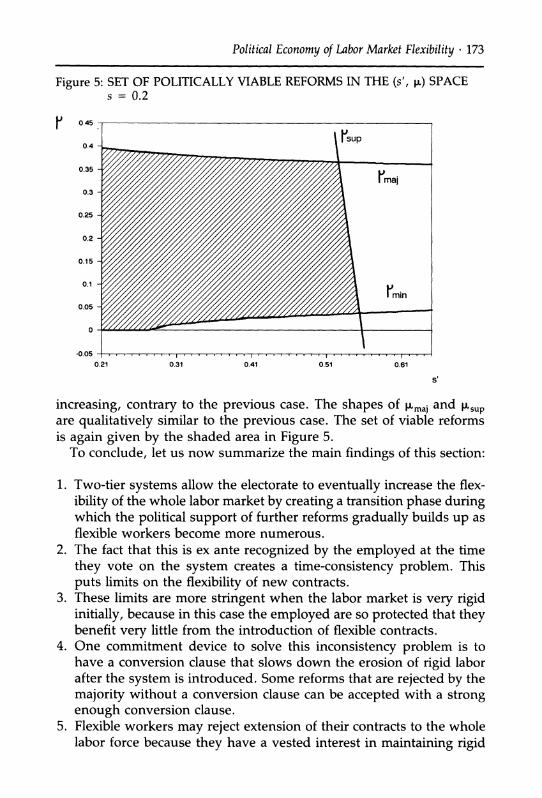
To summarize, under CCs the political viability of the sequence of reforms we have considered is subject to three constraints: ex ante ac-

ceptance of the two-tier system by the employed, reduction of rigid workers to a minority in finite time, and support of total reform by flexible workers. These three constraints are respectively represented by ix >- ILmin, Pl - IALmaj, and x -c xsup.

In order for one to get a firmer grasp on these constraints, Figures 4 and 5 plot the three constraints as a function of the reform firing rate s' for two values of the initial firing rate s: s = 0.1 and s = 0.2. X was chosen equal to 0.4, while all other parameters are the same as in Fig- ure 3.

At s = 0.1, ILmin is always strictly positive, so that no reform is im-

plementable without CCs. Lpmin is, however, very small, so that only a

very limited conversion clause makes reforms possible. Also, min is decreasing, suggesting that large increases in flexibility are more viable than small ones, at least over some range. Also, l,maj is smoothly de-

creasing with s', while usLup is steeply decreasing with s'. The set of viable reforms in the (s', ,L) plane is given by the shaded area in Figure 4. At s = 0.2, l,min is initially equal to zero. As s' increases, lxmin becomes

Figure 4: SET OF POLITICALLY VIABLE REFORMS IN THE (s', ,u) SPACE s = 0.1

0.11 0.21 0.31 0.41 0.51

S'


Figure 5: SET OF POLITICALLY VIABLE REFORMS IN THE (s', ,) SPACE s = 0.2

0.45

r"up 0.4

0.05 r,m., , ,aj,, . , , . , . , . . , , .

0.3

0.25

0.2

0.15

0.1

0.05 -

0

0.21 0.31 0.41 0.51 0.61

increasing, contrary to the previous case. The shapes of Imaj and ,sup are qualitatively similar to the previous case. The set of viable reforms is again given by the shaded area in Figure 5.

To conclude, let us now summarize the main findings of this section:

1. Two-tier systems allow the electorate to eventually increase the flex-

ibility of the whole labor market by creating a transition phase during which the political support of further reforms gradually builds up as flexible workers become more numerous.

2. The fact that this is ex ante recognized by the employed at the time

they vote on the system creates a time-consistency problem. This puts limits on the flexibility of new contracts.

3. These limits are more stringent when the labor market is very rigid initially, because in this case the employed are so protected that they benefit very little from the introduction of flexible contracts.

4. One commitment device to solve this inconsistency problem is to have a conversion clause that slows down the erosion of rigid labor after the system is introduced. Some reforms that are rejected by the majority without a conversion clause can be accepted with a strong enough conversion clause.

5. Flexible workers may reject extension of their contracts to the whole labor force because they have a vested interest in maintaining rigid

174 * SAINT-PAUL

Table 2 SHARE OF TEMPORARY JOBS IN TOTAL EMPLOYMENT (1989)

Country Percent

Belgium 5.1 Denmark 9.9 France 8.5 Germany 11.0 Italy 6.3 Netherlands 3.4 Portugal 18.7 Spain 26.6 United Kingdom 5.4

Source: OECD Employment Outlook, 1991.

contracts because of the conversion clause. As a result, for complete reform to be implemented in finite time, the conversion rate must not be too large.

The next section provides evidence on a policy experiment that is of

particular relevance for the theory outlined previously: the introduction of flexible contracts in Spain.

4. A Case Study: Spain Two-tier systems, where temporary contracts coexist with permanent ones, are prevalent in most European countries. As apparent in Table 2, the country that has gone farthest in the adoption of these contracts is Spain. In other countries, with the exception of Portugal, flexible contracts are only a small fraction of employment.

I will not deal in great detail with the Spanish experience, referring the reader to previous work (Bentolila and Saint-Paul, 1992).27 What we are interested in here is the political aspect of these reforms.

Temporary contracts were essentially introduced in 1984,28 after a decade of steady decline in employment (Fig. 6). This dramatic decline was largely due to the high pace of restructuring experienced by the

27. The key reference of interest to the specialist is Segura et al. (1991). The Spanish case has been analyzed in various other papers, including Bentolila and Dolado (1992) and Jimeno and Toharia (1991).

28. Legally speaking, they were introduced in 1980, but until 1984 their use was limited to seasonal jobs and temporary replacement of a permanent worker.


Figure 6: SPANISH EMPLOYMENT (MILLIONS) 13.2

13 -

12.8-

12.6 -

12.4 -

12.2 -

12-

11.8 -

11.6 -

11.4 -

11.2 -

11 -

10.8 i i i i i i i l 1 1 1

197419751976 19771978 1979 1980 1981 1982 1983 19841985 1986 19871988198919901991 1992

Spanish economy in the aftermath of Franco's death;29 in particular most

job losses were accounted for by the agricultural sector. Another factor is that the labor market, quite flexible under Franco, was made very rigid in 1976, with the introduction of very large firing costs. Last, oil shocks and the recession of the 1980s took their toll.

At the time of the introduction of flexible labor contracts, the unem-

ployment rate had reached a staggering 22%. Although labor unions were in principle opposed to these contracts, the political conditions for

implementing them were there. Because of the restructuring nature of

unemployment, the insiders felt that they were exposed to it because of the large rate of job destruction. At the same time, this same aspect generated a presumption that flexible labor contracts could have a large effect on the hiring rate, because there was scope for many new firms to be set up and grow.30 Therefore, the benefit to the employed of these contracts was substantial.

Unions were fully aware, however, that these contracts would gradually undermine their support. Although flexible workers had access to full union membership after six months, their interests were clearly different from those of the incumbent union members. As a result, since

29. See Bentolila and Blanchard (1990). 30. As reported by Lorenzo (1992, Fig. 1), the introduction of flexible contracts was pre-

ceded by a steady rise in the entry and exit rates in manufacturing from 1980 to 1984.

176 SAINT-PAUL

those contracts have been introduced, unions have forcefully repeated that their ultimate objective was their suppression. In accordance with the previous model, it is not surprising that unions obtained some limits on the use of these contracts. The major limit that was set was a conversion clause, according to which temporary contracts could only be renewed up to three years.

Despite that, after the introduction of these contracts, as much as 95% of the flow of new hires was on temporary terms. As a result, the share of employment on fixed-term contracts quickly rose to 30% of total employment. Because of the conversion clause, this share tended to stabilize in the early 1990s.31 These changes occurred amidst a climate of booming employment and growth, because of worldwide recovery in 1986-1989 and entry into the EEC. As shown in Bentolila and Saint-Paul (1992), there is a presumption that part of the employment boom is

explained by flexible labor contracts.32 The interesting thing about this figure of 30% is that if we add it to

the large number of unemployed people in Spain, we get a considerable mass of people in favor of labor market flexibility. Therefore, one may speculate that we are now not far from the critical time t* where further reforms can be passed. This is illustrated by this year's heated debate between the finance ministry, Carlos Solchaga, and union leaders over the reform of the contract system.

The reform proposed by the government is in line with what the model predicts, in the sense that there is now a drive for a homogeniza- tion of the whole labor market (i.e., an abandonment of the two-tier

system) and an increase in its flexibility compared to the permanent contract system. Although the reform is still vaguely formulated, the

government wants to develop part-time work (which is different from

temporary work, but more flexible than permanent contracts and entails no conversion clause), to facilitate the relocation of workers by firms into new plants, and considers lowering firing costs through the suppression of prior administrative approval. As a matter of fact, flexible contracts can now be renewed for up to four years instead of three.

The difference between this reform and the one I have considered earlier is that it will leave the labor market in a more rigid state than the now prevailing flexible tier of temporary workers. In my view, there

31. The following back-of-the-envelope computation can be made: A three-year conversion clause is equivalent to a value of ,L of about 0.3. If one assumes a quit rate p = 0.05 and a firing rate s = 0.10, the steady-state proportion of temporary workers in total employment is given by (p + s)/(I( + p + s) = 0.15/0.45 = 1/3.

32. We have also shown that the immediate effect of the two-tier system on total employment is larger than the long-run effect; thus, employment overshoots its long-run level.


are two reasons for this. First, although the unemployed and the flexible workers are very numerous, they are not quite a majority, and the

existing conversion clause prevents this stock from increasing further. As a result, the government is seeking some consensus on the issue, and for that reason is compelled to give some concessions to the holders of rigid contracts. Second, given the conversion clause, it may well be the case that flexible workers would also oppose a complete flexibiliza- tion of the labor market (i.e., L > ,sup). As a result, institutional unification occurs on the basis of an arrangement that is intermediate between

temporary and permanent contracts.

Despite these complications, the Spanish experience is a good illustration of the conditions under which a two-tier system is politically im-

plementable, and of the result that there will be a gradual building of

support for further increases in labor market flexibility.

5. On Complementarities: Theory and Evidence The earlier analysis has focused on a peculiar type of policy measure, i.e., an increase in labor market flexibility through a reduction in firing costs. It has, however, pointed to a principle that is more general: that in a world where the employed are a majority, there will be more political support for fighting unemployment when the employed are more vul- nerable to it. This in turn is likely to generate complementarities between the economic sphere and the political sphere: the more flexible the labor market, the more the employed are exposed to unemployment, and the

greater the political support to fight it.

Complementarities naturally arise in the analysis of two-tier systems as shown in Figure 3: At least over some range, the maximum level of

flexibility that is politically implementable is an increasing function of the initial level of flexibility. As a result, if the economy starts on the left of point A, it will be stuck at a low equilibrium where the very malfunctioning of the labor market makes any attempt to reform it politically unviable. By contrast, if the economy starts with a flexible enough labor market, it could eventually reach-through gradual two-tier reforms-an equilibrium like E where the market is more flexible and

unemployment possibly lower.

Complementarities are not limited to these types of measures. Sup- pose, e.g., that at t = 0 one votes on direct labor market measures that increase the hiring rate. More precisely assume that the hiring rate is now h(s) + m, where m is an index of the resources devoted to labor market programs, while the PDV of the tax cost to an employed of this program is equal to cm. As a result, the value of m that is most preferred

178 . SAINT-PAUL

by an employed individual is the one that maximizes:

(r + p + h(s) + m)w + s -( V(m) = - cm, (39)

(r + p)(r + p + s + h(s) + m)

where I have made use of Equation (8). It can be checked that V(m) is single-peaked in m. Provided there is an interior solution, the optimal value of m is the one that satisfies the first-order condition:

s(w - ) += c. (40) (r + p + s + h(s) + m)2(r + p)

If the employed are the majority, then Equation (40) in effect defines the level of m that will be agreed upon through majority voting. Com- plementarities are also apparent from Equation (40). The LHS of Equa- tion (40), the marginal value to the employed of an additional unit of labor market programs, is increasing in s at least for a range of small enough values of s; as a result, the equilibrium amount of resources devoted to labor programs will increase with turnover. This is also clear from solving Equation (40) in terms of m:

m = (s(w - w)/(c(r + p)))0.5 - (r + p + s) - h(s). (41)

Clearly, am/as > 0 for s small enough. Turnover is not the only dimension of labor market flexibility that

creates a link between unemployment and the value of being employed. Wage formation is also an important channel. Going back to Equation (39), suppose that the real wage w now depends on the degree of labor tightness. To simplify assume that w is just a function of the hiring rate:

w = w(h(s) + m); w' > 0. (42)

Then the first-order condition Equation (42) must be modified as follows:

s(w- w) (r + p)(r + p + s + h(s) + m)2

(h(s) + m + r + p)w'(h(s) + m) (r + p)(r + p + s + h(s))

c (4)


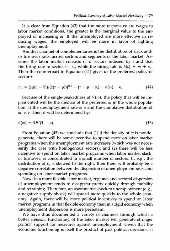
It is clear from Equation (43) that the more responsive are wages to labor market conditions, the greater is the marginal value to the em-

ployed of increasing m. If the unemployed are more effective in re-

ducing wages, the employed will be more in favor of fighting unemployment.

Another channel of complementaries is the distribution of slack and/ or turnover rates across sectors and segments of the labor market. As- sume the labor market consists of n sectors indexed by i and that the firing rate in sector i is si, while the hiring rate is h(s) + m + Ei. Then the counterpart to Equation (41) gives us the preferred policy of sector i:

mi = (si(w - w)l(c(r + p)))05 - (r + p + si) - h(si) - ei. (44)

Because of the single-peakedness of V(m), the policy that will be implemented will be the median of the preferred m in the whole popula- tion. If the unemployment rate is u and the cumulative distribution of mi is F, then it will be determined by:

F(m) = 0.5/(1 - u). (45)

From Equation (45) we conclude that (1) if the density of m is nonde-

generate, there will be some incentive to spend more on labor market

programs when the unemployment rate increases (which was not neces-

sarily the case with homogenous sectors); and (2) there will be less incentive to spend on labor market programs when labor market slack, or turnover, is concentrated in a small number of sectors. If, e.g., the distribution of Ei is skewed to the right, then there will probably be a

negative correlation between the dispersion of unemployment rates and

spending on labor market programs. Now, in a more flexible labor market, regional and sectoral dispersion

of unemployment tends to disappear pretty quickly through mobility and retraining. Therefore, an asymmetric shock to unemployment (e.g., a negative supply shock) will spread more quickly to the whole econ-

omy. Again, there will be more political incentives to spend on labor market programs in that flexible economy than in a rigid economy when

unemployment dispersion is more persistent. We have thus documented a variety of channels through which a

better economic functioning of the labor market will generate stronger political support for measures against unemployment. Given that the economic functioning is itself the product of past political decisions, it

180 SAINT-PAUL

is likely that we will observe a grouping of countries into "clubs," some of which are doing little about unemployment, with others having a full

array of measures.33

EVIDENCE ON COMPLEMENTARITIES

I now consider two types of evidence about complementarities. First, I test whether unemployment matters in political decision making essentially through its effect on the employed. My test is simple: If this is so, there will be more concern about unemployment when the rate of change of unemployment is high than when its level is high. This is because the current firing rate is much more correlated with the rate of change than with the level, and (abstracting from wage issues) it is essentially through the firing rate that unemployment affects the employed. So my empirical strategy is to correlate some measure of "concern" with the level and rate of change of unemployment, and test whether the second, rather than the first, is significant.

I have considered two measures of "concern." First, using a data set on elections in OECD countries between 1960 and 1990, I regress an indicator of an outcome favorable to the incumbent government on a set of economic variables, i.e., the levels and rates of change of unem-

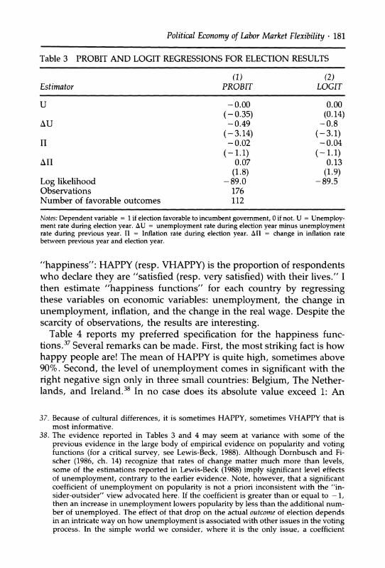
ployment and inflation.34 It is clear from Table 3 that only the change in unemployment comes

in significant. The unemployment rate, in particular, has essentially a zero coefficient.35 The coefficient of zero on the level of unemployment has strong implications: It means that one cannot reject the hypothesis of political hysteresis-after an increase in unemployment, there will be no force to bring unemployment back to some natural level through political discontent.

As a second measure of concern, I use satisfaction polls conducted in EEC countries since 1973.36 From this I constructed two measures of

33. This is indeed the picture that emerges if one compares Sweden, with its comprehen- sive system of labor market measures (mobility premia, centralized matching, relief jobs, solidaristic bargaining), with countries like France or Italy.

34. The data set is essentially the same as the one used by Alesina and Roubini (1992), itself based on Banks (1987) and Alt (1985). The variable used is a dummy equal to 1 if the outcome is favorable for the incumbent government and 0 if not. I have added Iceland and Greece and some more recent outcomes. Dummies for each country and each decade were included. The results were unaffected if one drops inflation or its change from the regression or adds the growth rate of consumption, output, or real wages.

35. Note also the low explanatory power of inflation. 36. These polls are reported in the periodical Eurobarometer Trends. Unfortunately, most

of these polls deal with issues like European unification. The one closest to my needs asks people whether they are satisfied with their lives.


Table 3 PROBIT AND LOGIT REGRESSIONS FOR ELECTION RESULTS

(1) (2) Estimator PROBIT LOGIT

U -0.00 0.00 (-0.35) (0.14)

AU -0.49 -0.8 (-3.14) (-3.1)

II -0.02 -0.04 (-1.1) (-1.1)

AIH 0.07 0.13 (1.8) (1.9)

Log likelihood - 89.0 - 89.5 Observations 176 Number of favorable outcomes 112

Notes: Dependent variable = 1 if election favorable to incumbent government, 0 if not. U = Unemploy- ment rate during election year. AU = unemployment rate during election year minus unemployment rate during previous year. I1 = Inflation rate during election year. An = change in inflation rate between previous year and election year.

"happiness": HAPPY (resp. VHAPPY) is the proportion of respondents who declare they are "satisfied (resp. very satisfied) with their lives." I then estimate "happiness functions" for each country by regressing these variables on economic variables: unemployment, the change in

unemployment, inflation, and the change in the real wage. Despite the scarcity of observations, the results are interesting.

Table 4 reports my preferred specification for the happiness functions.37 Several remarks can be made. First, the most striking fact is how happy people are! The mean of HAPPY is quite high, sometimes above 90%. Second, the level of unemployment comes in significant with the right negative sign only in three small countries: Belgium, The Nether- lands, and Ireland.38 In no case does its absolute value exceed 1: An

37. Because of cultural differences, it is sometimes HAPPY, sometimes VHAPPY that is most informative.

38. The evidence reported in Tables 3 and 4 may seem at variance with some of the previous evidence in the large body of empirical evidence on popularity and voting functions (for a critical survey, see Lewis-Beck, 1988). Although Dornbusch and Fi- scher (1986, ch. 14) recognize that rates of change matter much more than levels, some of the estimations reported in Lewis-Beck (1988) imply significant level effects of unemployment, contrary to the earlier evidence. Note, however, that a significant coefficient of unemployment on popularity is not a priori inconsistent with the "insider-outsider" view advocated here. If the coefficient is greater than or equal to -1, then an increase in unemployment lowers popularity by less than the additional number of unemployed. The effect of that drop on the actual outcome of election depends in an intricate way on how unemployment is associated with other issues in the voting process. In the simple world we consider, where it is the only issue, a coefficient

Table 4 ESTIMATES OF HAPPINESS FUNCTIONS

United Belgium Denmark Germany France Ireland Italy Netherlands Kingdom

Dependent variable Mean of H Constant

Trend

U

AU

n

ALog(W/P)

R2 DW

H 85.7 94.9

(58.7)

-1.06 (-6.1)

0.7 2.3

VH 94.7 38.0 (7.6) 0.76

(2.2) 0.11

(0.1) -1.92

(-1.9)

0.65 2.1

H 83.3 73.4

(27.2) 0.53

(2.9) -0.38

(-0.8) -1.6

(-2.2)

0.73 2.4

H 74.3 64.0

(16.2)

1.12 (3.1)

-3.8 (-3.3)

1.6 (2.5) 0.63 1.2

H 84.7 93.6

(33.9)

-0.63 (-3.5) -0.87

(-1.5)

0.41 (2.2) 0.63 1.8

Notes: t statistics in parentheses. Dependent variables: H = HAPPY, VH = VHAPPY. Source: Eurobarometer Trends, 1990. Variable definitions as in Table 3. ALog(W/P) = real wage growth.

VH 90.1 30.4 (8.7) 0.8

(4.0) -1.00

(-2.6)

H 84.0 89.5

(49.5)

-0.18 (-1.2)

H 65.9 45.2

(15.4)

2.43 (7.6)

-2.71 (-2.1)

0.8 1.4

-0.29 (-3.3)

0.52 1.8

0.45 1.8


additional unemployed person makes at most one person unhappy- presumably this person. Third, the coefficient on the change in unem-

ployment is significantly negative in four cases: France, Italy, Germany, and Denmark. These include the three major countries in the sample. The coefficient is always greater than -1.5 in all cases, reaching -4 in France. Therefore, these results fully confirm those from elections,39 and are consistent with the view that it is essentially through the employed's welfare that unemployment politically matters.

The second type of evidence I consider on complementarities is a direct test of the hypothesis through a cross-country correlation of some measure of the amount of resources devoted to fighting unemployment with some indicators of labor market flexibility.

The two main indicators I use are:

1. An index of "structural spending" (SS) against unemployment, taken as the share of GDP devoted to "active" labor market measures, divided by the unemployment rate.

2. An index of "cyclical spending" (CS), which is just the predicted long-run effect on the deficit/GDP ratio of a permanent increase in

unemployment by one percentage point, from a simple regression of deficit on unemployment and an AR1 term.

The labor market indicators I use are the rate of regional migration (MIG), a mismatch indicator for 1979 (MIS), the long-run and short-run

semi-elasticity of the real wage with respect to unemployment, esti- mated from a Phillips curve (SRPC and LRPC), the share of long-term unemployment (LTU), an index of regional concentration of unemployment (RCON), an index of real wage rigidity in the reduced form of the Phillips curve/labor demand system (RWR), an index of the separation rate (SEPA), and an index of the share of temporary contracts in the

economy (TEMP). Complementarities are then documented by examin-

ing the simple regression coefficient of CS and SS on these variables

greater than -1 suggests that the employed do not mind at all. Given that they are a majority, it is unlikely that the level of unemployment will affect the election outcome, even though unemployment is costly in terms of popularity. In other words, the findings from popularity functions are not inconsistent with the election outcome functions reported in Table 3. As a matter of fact, most of the estimates reported in Lewis-Beck are greater than -1. Also it should be noted that most of these specifica- tions do not test level vs. rate of change effects and that there is a general lack of robustness of popularity and voting functions.

39. Note also that inflation only matters in the United Kingdom, and that Northern Conti- nental Europe is increasingly happy: There is a positive time trend in Denmark, Ger- many, and The Netherlands.

184 SAINT-PAUL

over the sample of 23 OECD countries. Given that Sweden is an outlier (it has a very high value for both CS and SS), I also add a Swedish dummy to test for robustness whenever the coefficient is significant. Table 5 reports the matrix of these coefficients.

The evidence that emerges from Table 5 is mixed but tends to support the complementarity hypothesis. Whenever the coefficient is significant, it points toward more spending in more flexible countries. The only exception to that rule is the share of temporary contracts, suggesting, in accordance with the earlier analysis, that two-tier systems may act as a substitute for other measures in a very rigid country.

There are only a few variables, however, for which there is evidence of complementarities. These are:

* The regional migration rate MIG (positively correlated with both CS and SS, but this is due to Sweden).

* Long-run wage flexibility in the Phillips curve LRPC (positively correlated with CS and SS, even if Sweden is controlled for)

* Short-run wage flexibility in the Phillips curve SRPC (positively correlated with CS)

* The share of long-term unemployment LTU (negatively correlated with CS and SS, but this tends to disappear when Swedish dummy is included).

Table 5 REGRESSION COEFFICIENT MATRIX

Dependent variable CS CS SS SS

Swedish Dummy No Yes No Yes MIG 1.47** 1.4 0.19** 0.03 MIS -0.02 -0.00 SRPC 1.0** 0.97** 0.04 LRPC 0.24** 0.20** 0.03** 0.01** LTU -0.04* -0.03 -0.004* -0.001 RCON 0.6 0.13 SEPA -0.09 -0.00 RWR -1.9 -1.2 -0.27 -0.12* TEMP 0.06 -0.01**

Notes: Variables defined in text. *

Significant at the 10% level. ** Significant at the 5% level. Sources: For CS, OECD Economic Outlook. For SS, MIG, MIS, LTU, RCON, SEPA, and TEMP: OECD Employment Outlook. For SRPC, LRPC, and RWR: I use the estimates for AS and AD curves in the OECD in Layard, Nickell, and Jackman (1991).


An obvious problem is that of reverse causality: Maybe policies are

exogenous and we just estimate their effect on labor markets. It is difficult to evaluate the severity of this problem. Intuitively, it is certainly what explains the correlation between long-term unemployment and

spending. By contrast, it is more doubtful that policies affect real wage flexibility so as to generate the observed correlation.40 Insofar as they are accommodative, they can well increase real wage rigidity,41 in which case the regression coefficients of CS and SS on SRPC and LRPC under- estimate the effects of labor market flexibility on the political support to

fight unemployment. Hence, it is essentially through wage formation that complementa-

rities seem to work. In particular, turnover and concentration do not seem to have any impact.

6. Conclusion and Directions for Future Research The present paper has concentrated on a limited, although very important in my view, aspect of the political issues of unemployment in

Europe. Clearly, the politico-economic analysis of persistent unemployment encompasses a much broader and richer set of issues. Several

important factors remain to be analyzed: Why are there not more incentives to organize the unemployed as a pressure group? Are there con- flicts of interest among various subgroups within the unemployed (women, the young, the long-term unemployed, etc...)? To what extent can the employed collectively raise their bargaining power through the political system, and can this generate persistence?42

The general message of the paper, that there is not much concern about unemployment, might seem crazy. After all, don't governments lose popularity and elections because of unemployment? Aren't politi- cians always talking about "more jobs"?

The answer is that this may well be true in the short run, when there is precisely a close association between rising unemployment and the employed's welfare. In the long-run, however, as unemployment stabi- lizes at a high level, unemployment ceases to be an issue, as Table 1 as well as the evidence in Section 5 makes clear.

40. See Calmfors (1992) for a critique of the view that labor market measures have increased wage flexibility in Sweden.

41. See Calmfors and Horn (1986). 42. This would occur in a way essentially similar to the insider effect pointed out by

Blanchard and Summers (1986).

186 . SAINT-PAUL

REFERENCES

Alesina, A. (1987). Macroeconomic policy in a two-party system as a repeated game. Quarterly Journal of Economics.

(1988). Macroeconomics and politics. NBER Macroeconomics Annual. ,and N. Roubini. (1992). Political cycles in OECD economies. Review of

Economic Studies. Alt, J. (1985). Political parties, world demand, and unemployment: Domestic

and international sources of economic activity. American Political Science Review.

Banks, A. (1987). Political handbook of the world. Bean, C. R. (1993). European unemployment: A survey. Journal of Economic

Literature. Bentolila, S., and G. Bertola. (1990). Firing costs and labor demand: How bad

is Eurosclerosis? Review of Economic Studies 57:381-402. , and 0. Blanchard. (1990). Spanish unemployment. Economic Policy. , and J. Dolado. (1992). Who are the insiders? Wage-setting and tempo-

rary contracts in Spanish manufacturing. Mimeo, CEMFI. , and G. Saint-Paul. (1992). The macroeconomic impact of flexible labor

contracts, with an application to Spain. European Economic Review 36:1013- 1053.

Bertola, G. (1990). Job security, employment, and wages. European Economic Review 34:851-880.

Blanchard, 0., and P. Diamond. (1989). The Beveridge curve. Brookings Papers on Economic Activity.

, and L. Summers. (1986). Hysteresis and the European unemployment problem. NBER Macroeconomics Annual.

Burda, M. (1991). Insider effects and union wage determination. Economica. Burda, M., and C. Wyplosz, (1990). Gross labor market flows in Europe: Some

stylized facts. DELTA Working Paper. Calmfors, L. (1992). Lessons from the macroeconomic experience of Sweden.

Working paper #522, IIES, Stockholm. , and H. Horn. (1985). Classical unemployment accommodation policies

and the adjustment of real wages. Scandinavian Journal of Economics 87:195-212. Cohen, D. (1988). What caused the rise of conservatism? A French view. Eco-

nomic Policy. Dewatripont, M., and G. Roland. (1992). Economic reform and dynamic political

constraints. Review of Economic Studies 59:703-730. Dornbusch, R., and S. Fischer. (1986). Macroeconomics. 3rd ed. McGraw Hill. Eurobarometer. (1990). Eurobarometer trends. Hibbs, D. A. (1982). The political economy of industrial democracy. Cambridge, MA:

Harvard U. Press. Jimeno, J., and L. Toharia. (1991). Productivity and wage effects of fixed-term

employment: Evidence from Spain. Mimeo, U. de Alcala de Henares. Layard, R., S. Nickell, and R. Jackman. (1990). Unemployment. Oxford U. Press. Lewis-Beck, M. S. (1988). Economics and elections. Ann Arbor, MI: U. of Michigan

Press. Lindbeck, A., and D. Snower. (1989). The insider-outsider theory of employment.

Cambridge, MA: MIT Press. Lorenzo, M. J. (1992). Flujos de Entrada y Salidas de Establecimientos en el

Sector Manufacturero Espafiol. Mimeo.

Comment 187

Mortensen, D., and C. Pissarides. (1992). Job creation and job destruction in the theory of unemployment. Mimeo.

Pissarides, C. (1989). Equilibrium unemployment theory. London: Basil Blackwell. Piketty, T. (1992). Voting over redistributive tax schedules. Mimeo, DELTA. OECD. Economic Outlook, Paris. OECD. Employment Outlook, Paris, 1988, 1989, 1990, 1991, 1992. Rebitzer, J., and L. Taylor. (1991). A model of dual labor markets when product

demand is uncertain. Quarterly Journal of Economics 106:1373-1383. Roland, G., and T. Verdier. (1991). Privatization in Eastern Europe: Irreversibil-

ity and critical mass effects. DELTA working paper #91-21. Saint-Paul, G. (1991). Dynamic labor demand with dual labor markets. Economics

Letters 36:219-222. . (1992a). Are the unemployed unemployable? CEPR discussion paper

#689. . (1992b). The high unemployment trap. CEPR discussion paper #670.

Segura, J., F. Duran, L. Toharia, and S. Bentolila. (1991). Analysis de la Contrata- cion Temporal en Espana. Madrid: Ministerio de Trabajo.

Comment ANDREW ATKESON University of Chicago

Gilles Saint-Paul has built his discussion of the political economy of labor market flexibility on the premise that there is a conflict between attitudes of the employed and the unemployed toward taxes on the termination of employment. His central argument is that taxes on the termination of employment are beneficial to the employed because they extend the expected duration of existing jobs and are harmful to the

unemployed because they reduce the probability that the unemployed find employment. The critical step in this argument is presented in

Equation (10) of the paper. In examining this equation, we see that Saint- Paul has taken care to model the impact of employment termination taxes on the expected duration of employment and unemployment, but we also see that he has given no accounting at all of who pays the direct cost of the employment termination taxes themselves.

In this comment, I re-examine the impact of employment termination taxes on employment and welfare under the assumption that it is the employed who bear the direct cost of the employment termination tax. With this assumption, it becomes clear that there is no conflict between the employed and unemployed on reducing employment termination taxes because any reduction of these taxes necessarily leads to a Pareto improvement. Once we view a tax on the termination of employment

Comment 187

Mortensen, D., and C. Pissarides. (1992). Job creation and job destruction in the theory of unemployment. Mimeo.

Pissarides, C. (1989). Equilibrium unemployment theory. London: Basil Blackwell. Piketty, T. (1992). Voting over redistributive tax schedules. Mimeo, DELTA. OECD. Economic Outlook, Paris. OECD. Employment Outlook, Paris, 1988, 1989, 1990, 1991, 1992. Rebitzer, J., and L. Taylor. (1991). A model of dual labor markets when product

demand is uncertain. Quarterly Journal of Economics 106:1373-1383. Roland, G., and T. Verdier. (1991). Privatization in Eastern Europe: Irreversibil-

ity and critical mass effects. DELTA working paper #91-21. Saint-Paul, G. (1991). Dynamic labor demand with dual labor markets. Economics

Letters 36:219-222. . (1992a). Are the unemployed unemployable? CEPR discussion paper

#689. . (1992b). The high unemployment trap. CEPR discussion paper #670.

Segura, J., F. Duran, L. Toharia, and S. Bentolila. (1991). Analysis de la Contrata- cion Temporal en Espana. Madrid: Ministerio de Trabajo.

Comment ANDREW ATKESON University of Chicago

Gilles Saint-Paul has built his discussion of the political economy of labor market flexibility on the premise that there is a conflict between attitudes of the employed and the unemployed toward taxes on the termination of employment. His central argument is that taxes on the termination of employment are beneficial to the employed because they extend the expected duration of existing jobs and are harmful to the

unemployed because they reduce the probability that the unemployed find employment. The critical step in this argument is presented in

Equation (10) of the paper. In examining this equation, we see that Saint- Paul has taken care to model the impact of employment termination taxes on the expected duration of employment and unemployment, but we also see that he has given no accounting at all of who pays the direct cost of the employment termination taxes themselves.

In this comment, I re-examine the impact of employment termination taxes on employment and welfare under the assumption that it is the employed who bear the direct cost of the employment termination tax. With this assumption, it becomes clear that there is no conflict between the employed and unemployed on reducing employment termination taxes because any reduction of these taxes necessarily leads to a Pareto improvement. Once we view a tax on the termination of employment

188 . ATKESON

as a tax on the employment relationship, the intuition for this result is

quite simple. An employment relationship of any fixed duration is more valuable to the parties involved if its termination is not taxed. Thus, as

long as employer and employee choose the duration of employment to maximize the surplus in the employment relationship, the surplus to be divided between the parties to the employment relationship must rise when employment termination taxes are reduced, even if, in equilibrium, employer and employee decide to reduce the duration of em-

ployment in response to the tax reduction. In the remainder of this comment, I present a simple general equilib-

rium model of the impact of employment termination taxes on welfare and employment to illustrate the argument that a reduction of those taxes is a Pareto improvement.

1. The Model Consider an infinite horizon economy populated by a continuum of

agents. Assume that all agents are risk neutral and have discount factor R < 1. Agents produce output in the context of matches with existing production technologies. Assume that at each date t - 0, a new production technology becomes available. Index the production technologies available to agents at date t by T = -oo, ..., -1,0,1,2, . . . t. Agents begin each period t either matched with an existing technology T < t or in the pool of agents searching for a new match with the new technology T = t.

All agents in the search pool at date t draw a match of random quality with technology T = t. At the beginning of date t + 1, these agents discover the quality of that match. Let the quality of a match be indexed

by A E {A1, A2, . . ., Al}, with Al < A2 < . . . < AJ. Let F'j be the

probability that a new match is of quality Aj. Upon discovering the

quality of their new match, these agents then choose either to accept or

reject the match. Agents who accept their new match of quality A with

technology T = t at date t + 1 can produce AGT each period for as many periods as they choose to remain with that match, where G > 1 and RG < 1. In particular, these agents in new matches may choose to produce in period t + 1, quit the match, and return to the search pool in period t + 2. Agents who refuse their new match at date t + 1 return to the search pool in period t + 2.

Agents who begin period t in an existing match of quality A with

technology T < t produce AGT in period t and then choose whether to remain with that match or to quit that match and return to the search

pool at date t + 1. We assume that the government imposes a tax on

Comment 189

agents who leave matches. Agents who leave a match in period t are taxed FGt+ in period t + 1. For simplicity, I assume that the tax is a bureaucratic cost of terminating employment so that no actual tax revenue is collected. I will discuss later how the results change when the tax generates revenue that is rebated to agents in a lump sum fashion.

We solve the model as follows. Let Vs be the discounted expected utility of being in the search pool at date t. It can be shown that Vt = VSGt where Vs is the utility of being in the search pool at date 0. Agents who accept matches of quality A with technology T at date t = T + 1 choose the number of periods n - 1 to continue in their match to solve

n max Y Rs-1 GTA + RnGt+n(VS - F). (1) n>l s=l

Let n(A) be the solution to this problem. Agents who accept a match of

quality A with technology T leave that match after producing at date 7 + n(A) and rejoin the search pool at date T + n(A) + 1. If n(A) - 2, then n(A) is the largest value of n such that

A + G"(RG)(V - F) -Gn(Vs- F). (2)

The left-hand side of Equation (2) is the utility of producing in period T + n and then leaving the match to join the search pool in period 7 + n + 1. The right-hand side of Equation (2) is the utility of having left the match in period T + n - 1 and joining the search pool in period T + n. Equation (2) implies that, holding Vs constant, increasing the employment termination tax F prolongs matches. We will see later that

increasing F also decreases Vs, so that this effect persists in general equilibrium.

For agents who drew new matches at date t - 1, define the value of

discovering at date t that the quality of that match is A as Vt(A) = GtV(A), where

n

V(A) = max (RG)Vs, max E Rs-1 G-1 A + (RG)(V - F) . (3) n>l s=l

The first term on the right-hand side of Equation (3) is the value of refusing the match and rejoining the search pool the next period, while the second term is the value of accepting the match and producing the optimal number of periods. We finish the solution with the equation

Vs = RG V(Aj)i. (4)

J

190 ATKESON

To evaluate the impact of taxes on firing on welfare, we begin with the following lemma.

Lemma 1: Vs declines in F. Proof. Define the function T: R -> R by

T(v) = RG Ea rjmax (RG)v, max Y Rs- G-1Aj + (RG)"(v - F) . D j n>l s=l

Clearly Vs is a fixed point of T. The function T is continuous, and it maps values of v e [A1R/(1 - R), AiRG/(1 - RG)] back into this interval. Thus, T has a fixed point on this interval. Furthermore, we show that for all values v1 > v2, T(v1) - T(v2) - (RG)2(V1 - v2) as follows. Consider the terms that comprise T(v) one at a time. Let TJ(v) be defined

~- ~~~n TI(v) = RG max (RG)v, max , Rs-1 G -A + (RG)n(v - F)

n>l s=l

Assume TJ(vl) = (RG)2vl. By definition TJ(v2) - (RG)2v2. Now assume

TJ(vl) = RG Rs-1 G-1Aj + (RG)n(vl - F)

s=1

where n i is the solution to

n

max Y R-1G-1Aj + (RG)n(vl - F). n>-1 s=l

By definition,

nJ, Ti(v2) RG C R- G-1Aj + (RG) n(v2- F).

s=l

Because T(v) = Ej rrj T (v), the result holds. Thus, T has slope less than one so it has a unique fixed point. Observe that increasing F must reduce T(v). Thus, because T has slope less than one, increasing F must reduce the fixed point VS.II

From Lemma 1, we see that the unemployed are in favor of lowering employment termination taxes. Given the result in Lemma 1, it is also clear from the problem (1) defining n(A) that lowering F must also increase the welfare of those employed in existing matches. Therefore,

Comment ? 191

the vote to reduce employment termination taxes is unanimous. In con-

trasting this result with the result in the paper by Saint-Paul, we see that he did not subtract the employment termination tax from the welfare of the employed. In particular, he defines the welfare of the employed as

n(A)

Rs-i GTA + Rn(A) GT+n(A) V. (5) s=l

Because it is true that n(A) increases as we increase F, he is able to get the result that the lowering F lowers n(A) and, thus, by his accounting, lowers the welfare of the employed as long as Vs does not rise too much.

We can solve for the impact of employment termination taxes on

employment in the steady state as follows: Let B denote the number of

agents in the search pool in the steady state. Let m(A) be an indicator variable indicating whether agents accept a match of quality A or reject such a match. In particular, let m(A) = 0 if agents reject a match of

quality A and m(A) = 1 otherwise. In the steady state, for all A such that m(A) = 1, there will be 7r(A)B agents in matches of quality A with

technology T at date T + s, for all s = 1, 2, . . . , n(A). In addition, there will be Ej j(1 - m(Aj)) B agents who refuse new matches at each date. If we normalize the number of agents to 1, we get

I(_1) B = (I + m(A1)n(A)r + E (1 - m (Aj)) rj)

The number of unemployed in every period is the sum of those in the search pool and those who reject new matches: B + Ej Trj (1 - m(Aj))B. Through computation, it appears that raising F raises unemployment for low values of F and lowers unemployment for high values of F. This is because, at F = 0, agents accept all new matches and operate them for at least one period. As F rises, low-quality matches quickly become unprofitable, so the rate at which new matches are rejected rises quickly. As F gets large, only high-quality matches are accepted. Further increases in F simply extend the duration of these high-quality matches.

If we modify this model to have the government collect revenues from the employment termination tax and redistribute those revenues to all agents in a lump sum fashion, agents attitudes toward lowering the employment termination tax change. In particular, in computation it appears that agents who are in the search pool or who have recently joined matches of a long duration tend to be against lowering the tax

192 SOLOW

on employment termination, while those who are close to leaving their current match tend to be in favor of lowering these taxes. This result

appears to arise from consideration of the incidence of the tax: Those who are close to leaving an existing match have a high tax burden in

present value terms, while those who are unemployed or at the beginning of a long match have a low tax burden in present value terms.

2. Conclusion

In this note, I have examined the impact of employment termination taxes on welfare and employment in a general equilibrium model in which workers bear the full cost of the tax at the time that the tax is

paid. In this model, lowering employment termination taxes is a Pareto

improvement. If one is to build carefully an argument that the employed dislike reductions in employment termination taxes, one must consider how it is that termination taxes on employment have a large enough effect on the division of the surplus of the employment relationship so as to deliver more surplus to the worker despite the fact the tax itself reduces the total surplus to be divided. I leave such a task to future work.

Comment ROBERT M. SOLOW Massachusetts Institute of Technology

This is a very well thought out paper. It combines three recent trends in macroeconomics. The first is the modeling of gross flows in the labor market: into and out of employment, unemployment, and the labor force. This is unambiguously a good thing. The second is intertemporal- equilibrium modeling of unemployment, as if unemployment were a sort of occupation. On the whole, this is a bad thing, I think. The third is the new sort of political-economic modeling. I have no settled opinion about this. The combined exercise is interesting. It is applied to a very favorable case, i.e., Spain. How wide its field of applicability will turn out to be is anyone's guess.

The basis of the model is Equation (3), which makes the hiring rate a function of the separation rate. This function is assumed to be increas-

ing and concave. The slope is straightforward. It is assumed that s is a

decreasing function of firing costs (F) for obvious reasons. Also, h is a

decreasing function of F because employers know it will be harder to

192 SOLOW

on employment termination, while those who are close to leaving their current match tend to be in favor of lowering these taxes. This result

appears to arise from consideration of the incidence of the tax: Those who are close to leaving an existing match have a high tax burden in

present value terms, while those who are unemployed or at the beginning of a long match have a low tax burden in present value terms.

2. Conclusion

In this note, I have examined the impact of employment termination taxes on welfare and employment in a general equilibrium model in which workers bear the full cost of the tax at the time that the tax is

paid. In this model, lowering employment termination taxes is a Pareto

improvement. If one is to build carefully an argument that the employed dislike reductions in employment termination taxes, one must consider how it is that termination taxes on employment have a large enough effect on the division of the surplus of the employment relationship so as to deliver more surplus to the worker despite the fact the tax itself reduces the total surplus to be divided. I leave such a task to future work.

Comment ROBERT M. SOLOW Massachusetts Institute of Technology

This is a very well thought out paper. It combines three recent trends in macroeconomics. The first is the modeling of gross flows in the labor market: into and out of employment, unemployment, and the labor force. This is unambiguously a good thing. The second is intertemporal- equilibrium modeling of unemployment, as if unemployment were a sort of occupation. On the whole, this is a bad thing, I think. The third is the new sort of political-economic modeling. I have no settled opinion about this. The combined exercise is interesting. It is applied to a very favorable case, i.e., Spain. How wide its field of applicability will turn out to be is anyone's guess.

The basis of the model is Equation (3), which makes the hiring rate a function of the separation rate. This function is assumed to be increas-

ing and concave. The slope is straightforward. It is assumed that s is a

decreasing function of firing costs (F) for obvious reasons. Also, h is a

decreasing function of F because employers know it will be harder to

Comment 193

lay off workers if that were to become desirable. Thus, h(s), parametri- cally, is increasing. The concavity comes from general reasoning, al-

though it seems to me that a convex-concave shape is more likely. Now think about h(s). There are three sources of separations. (a)

There are quits: One would expect h to be higher when quits are more

frequent. (b) There is dynamic reshuffling of jobs as demand shifts between industries and regions: Here too hiring and separation should rise and fall together. (c) There are business-cycle events as real aggre- gate demand varies. Here you would expect h to be lower when s is

higher. So there is a whole aspect of life to which the model does not

apply. This suggests that anyone who wants to use the model empiri- cally should take cyclical unemployment out of the data.

The application of the model to two-tier wage systems is neat and

interesting. It must be an idealized two-tier system because it has the obvious implication that it will be favored by the employed if and only if it is favored by the unemployed. The intuition is that, in the model, the two-tier system does no harm to the employed as long as they stay employed. When they become unemployed, they are like other

unemployed workers, so they will be better off if the generic unem-

ployed worker is better off. When the two-tier system was proposed by U.S. airlines, the Air

Line Pilots Association (ALPA) opposed it. They were worried about eventual control of the union, which corresponds in Saint-Paul's model to the creation of a political majority in favor of a competitive labor market.

Spain is probably a good case study for this kind of model. The U.S. airline industry is less favorable. Clearly the ALPA feared that low-wage workers would eventually become a majority and attack the privileges of insiders. So the incumbent insiders bring pressure on employers to assimilate low-wage workers in the basic contract. The two-tier system may tend to erode and disappear.

In fact, when United Airlines and American Airlines finally negoti- ated two-tier systems with their employees, the contracts called for the

phasing-out of the system after a stated number of years. This provision has the effect of limiting the weight of low-tier employees in the total, preserving the influence of the original high-tier workers. In fact, the closure date is approaching for American Airlines. It will have to absorb the low-tier workers into the high tier, the result being an increase in labor costs at a time when the airlines are unprofitable.

The institution of a two-tier system in a single industry is not the same thing as doing it on an economywide basis. But I think the airline

experience is a warning that the simple political-economy results may

194 SOLOW

not apply. Perhaps this should be interpreted as meaning that the stable "inflexible" equilibrium, as Saint-Paul describes it, may be a very com- mon case. The process that leads to it will contain a lot of information about the dynamics of the labor market.

The conclusions reached at the end of Section 3 are reasonable. Here, too, it would be interesting to consider the sorts of shocks that would lead from a "flexible" equilibrium to a "rigid" one.

Discussion

Alberto Alesina suggested another labor market reform that may in fact be feasible: the reduction of unemployment compensation. He wondered if Saint-Paul had any results concerning this reform. Saint-Paul responded that with such a reform it is important to distinguish between partial and general equilibrium effects. In the partial equilibrium, both the employed and the unemployed would suffer from a decrease in unemployment compensation, so everyone would oppose it. In the general equilibrium, of course, unemployment compensation is fi- nanced by taxes so that the employed may in fact favor a reduction. Also, issues of bargaining power arise, and the presence of unemployment insurance increases the workers' bargaining power so that they may not favor a reduction. Ariel Pakes noted that risk aversion may be another reason why reducing unemployment insurance is not a popular way of making labor markets more flexible. He quipped that this discussion reminded him of a remark by Nicholas Kaldor, who said he could easily stop the inflation caused by central bankers: Execute them. More generally, he wondered if the results of the paper would hold up if individuals had concave utility functions.

Alesina also expressed a concern echoed by others: If the elimination of the firing costs can improve welfare, why are the firing costs there in the first place? Julio Rotemberg suggested that there may be two reasons for the presence of firing costs. First, they may have been insti- tuted to allow workers to accumulate general human capital. Alterna- tively, and this is consistent with the model, firing costs may have been imposed by the workers after they were hired in order to extract rents from the firm. But if that is how the workers obtained the firing costs in the first place, they are less likely to vote to reduce them now.

Marty Eichenbaum wondered why the United States is not afflicted by the same high unemployment problems as Europe. Saint-Paul responded that the U.S. experience fits well with the theory. The United

194 SOLOW

not apply. Perhaps this should be interpreted as meaning that the stable "inflexible" equilibrium, as Saint-Paul describes it, may be a very com- mon case. The process that leads to it will contain a lot of information about the dynamics of the labor market.

The conclusions reached at the end of Section 3 are reasonable. Here, too, it would be interesting to consider the sorts of shocks that would lead from a "flexible" equilibrium to a "rigid" one.

Discussion

Alberto Alesina suggested another labor market reform that may in fact be feasible: the reduction of unemployment compensation. He wondered if Saint-Paul had any results concerning this reform. Saint-Paul responded that with such a reform it is important to distinguish between partial and general equilibrium effects. In the partial equilibrium, both the employed and the unemployed would suffer from a decrease in unemployment compensation, so everyone would oppose it. In the general equilibrium, of course, unemployment compensation is fi- nanced by taxes so that the employed may in fact favor a reduction. Also, issues of bargaining power arise, and the presence of unemployment insurance increases the workers' bargaining power so that they may not favor a reduction. Ariel Pakes noted that risk aversion may be another reason why reducing unemployment insurance is not a popular way of making labor markets more flexible. He quipped that this discussion reminded him of a remark by Nicholas Kaldor, who said he could easily stop the inflation caused by central bankers: Execute them. More generally, he wondered if the results of the paper would hold up if individuals had concave utility functions.

Alesina also expressed a concern echoed by others: If the elimination of the firing costs can improve welfare, why are the firing costs there in the first place? Julio Rotemberg suggested that there may be two reasons for the presence of firing costs. First, they may have been insti- tuted to allow workers to accumulate general human capital. Alterna- tively, and this is consistent with the model, firing costs may have been imposed by the workers after they were hired in order to extract rents from the firm. But if that is how the workers obtained the firing costs in the first place, they are less likely to vote to reduce them now.

Marty Eichenbaum wondered why the United States is not afflicted by the same high unemployment problems as Europe. Saint-Paul responded that the U.S. experience fits well with the theory. The United

Discussion 195

States has a very flexible labor market, and, therefore, there is a great deal of political support for fighting unemployment. Eichenbaum then asked why the U.S. employed did not support an increase in firing costs, particularly during times of recession. Solow suggested that the absence of strong trade unions might be part of the explanation.

David Romer expressed concern that the wrong question is being asked about political reform. With 5% of GNP to work with every year, it should not be difficult to come up with a number of political reforms that would attract a majority of voters. Instead, the real puzzle is why people do not vote for things that make them better off. As another

example, Romer mentioned California water policy.

http://www.jstor.org/stable/3585029?origin=JSTOR-pdf

http://www.jstor.org/page/info/about/policies/terms.jsp

http://www.jstor.org/action/showPublisher?publisherCode=ucpress

Date post:	24-Aug-2019
Category:	Documents
Upload:	dohanh
View:	214 times
Download:	0 times

On the Political Economy of Labor Market Flexibility · Gilles Saint-Paul CERAS AND DELTA, PARIS,...

Documents