On the probability and spatial distribution of

ocean surface currents

Yosef Ashkenazy ∗

Solar Energy and Environmental Physics, BIDR,

Ben-Gurion University, Midreshet Ben-Gurion, Israel

Hezi Gildor

The Fredy and Nadine Herrmann Institute of Earth Sciences,

The Hebrew University of Jerusalem, Jerusalem, 91904, Israel

∗Corresponding author address: Yosef Ashkenazy, Solar Energy and Environmental Physics, BIDR, Ben-

Gurion University, Midreshet Ben-Gurion, Israel.

E-mail: ashkenaz@bgu.ac.il

ABSTRACT

Insights into the probability distribution of ocean currents is important for

various applications such as the chance to encounter extreme events which may

affect, for example, marine construction, and for estimating the energy that can

be extracted from the ocean. In addition, for devising better parameterizations

for submesoscale mixing, which present climate models cannot resolve, one should

understand the velocity distribution and its relation to the various forcing of sur-

face ocean circulation. Here we investigate the probability distribution of surface

currents measured by high-frequency radar. Our results show that the distri-

bution of ocean currents’ speed can be approximated by a Weibull distribution.

Moreover, we demonstrate the existence of spatial variations of the scale and

shape parameters of the Weibull distribution over a relatively small region of

only a few kilometers. We use a simple surface Ekman layer model to try to

understand this spatial variability; we find that when forced by local winds this

model does not reproduce the observations. We show that Gaussian noise added

to the zonal and meridional components of the bottom geostrophic currents have

only a slight effect on the surface currents distribution, while noise added to the

components of the local wind (mimicking wind gusts) have much greater effect

on the distribution of surface currents, suggesting that wind spatial and tempo-

ral variability underlay the observed spatial variability of the parameters of the

Weibull distribution.

1

1. Introduction

Ocean currents are the cumulative result of local and remote factors, including winds,

buoyancy fluxes, tides, and many types of waves; the influence of these forces on ocean

currents is not trivial. While wind distribution has been studied extensively in the past

(e.g., Seguro and Lambert 2000), the distribution of ocean currents had received only a little

attention (Chu 2008). In this work we analyze the probability distribution of ocean surface

currents measured by High-Frequency (HF) radar. We show that the distribution of surface

ocean current speeds may be approximated by Weibull distribution, and that the parameters

of the distribution vary over relatively small spatial scales of the order of a few kilometers.

Using a simple surface Ekman layer model, we show that this variability may be linked to

wind spatial and temporal variability.

The motivations behind deriving this distribution are: (1) for many practical applications

it is necessary to know the current distribution, for example when planning marine construc-

tion. (2) There is a need to parameterize sub-grid ocean mixing in numerical models. Due

to limited computer power, present day ocean and climate models usually resolve processes

on scales down to a few kms, and have to parameterize processes on smaller scales.

To better parametrized submesoscale ocean mixing, we should know the probability dis-

tribution function of surface currents. While it was shown before that the distribution of

surface currents speed follow the Weibull distribution (e.g., Chu 2008) on the mesoscale and

larger scales, here we demonstrate this relation for the submesoscale. (3) Knowledge of the

distribution of the currents can serve as a benchmark for ocean models, i.e. one can test

whether these models reproduce the same statistics of the observed currents. (4) Last, it is

2

possible to learn about the probability of extremely severe currents from their distribution,

a fact that may help to more efficiently manage maritime trade, breakwaters, ports, etc.

Previous studies either used a limited number of point measurements and therefore had

a limited spatial and temporal sampling (e.g., Chu 2008) or used velocities from numerical

models (Bracco et al. 2003). Other studies used currents derived from satellite altimeter

(Gille and Smith 1998, 2000; Chu 2009), and found that surface current speed follows the

Weibull distribution; these satellite data were collected approximately every five days and

had 1◦×1◦ spatial resolution. Here we extract the distribution of surface currents using a

data set of surface currents measured by HF radar. This data set is characterized by a long

time series (several years) with fine temporal (half an hour) and spatial (∼300 m) resolutions.

These submesoscale radar observations therefore fill an important gap between point mea-

surements (by current meter or Acoustic Doppler Current Profiler) and mesoscale data (a

few tens of kilometers). As mentioned above, we show that surface current distribution may

be approximated by the Weibull distribution. Mapping of the scale and shape parameters

of the Weibull distribution over a domain scale of 10-20 kms indicates significant changes in

these distribution parameters.

In the next section (Sec. 2) we describe the study region and the data set used. In Sec. 3

we review a few characteristics of the Weibull distribution. The results are presented in Sec.

4. A simple surface Ekman layer model is than used to study the origin of the distribution

of surface currents (Sec. 5). We conclude in Sec. 6.

3

2. Measurements methods and studied region

a. Study region

The northern terminus of the Gulf of Eilat is a nearly rectangular, deep (∼700 m, Fig. 1),

and semi-enclosed basin in the northeast region of the Red Sea. The Gulf of Eilat (referred

to hereafter as ’the gulf’) is bounded by a desert mountain range that steers the persistent

northerly wind along its main axis (Berman et al. 2003). The circulation in the gulf has

wind-driven, tidal, and thermohaline components. The tidal component is dominated by

the semi-diurnal (M2) peak forced by the flux of water through the Straits of Tiran (Genin

and Paldor 1998; Monismith and Genin 2004; Manasrah et al. 2006). The surface flow is

most of the time quite complex as demonstrated in Fig. 1a although occasionally a large

(much of the domain) spatially coherent eddy (Fig. 1b) fills the domain (?).

Cold, dense water from the world ocean cannot flow into the Gulf of Eilat because it is

blocked by the shallow sill (137 m) near Bab el Mandeb and the shallow sill (240 m) of the

Tiran Strait (?). Consequently, stratification across the entire water column in the gulf is

relatively weak and deep water forms in situ. The weak density stratification breaks down in

winter as a result of surface cooling and evaporation, and deep water forms (??Biton et al.

2008). In FebruaryMarch we find vertical homogeneity in temperature and salinity reaching

a depth of a few hundred meters and sometimes down to the bottom, with new stratification

beginning to form in March (?). In summer the Gulf is stratified with an upper warm layer

of up to 200m depth overlying a homogeneous deeper layer. Accordingly, the first baroclinic

Rossby radius changes seasonally, ranging from 6 km to 20 km

The configuration and dimensions (six by ten km basin) of the northern gulf (Fig. 1)

4

enables observation of surface currents at a very high spatial and temporal resolution using

HF radar, rendering this gulf a unique natural laboratory for studying submesoscale mixing

processes. The HF radars provide two dimensional maps of surface currents every thirty

minutes with a spatial resolution of about 300 m.

During most of the year the wind in Eilat region blow from the north, with a small easterly

component; see below. Rarely, there are strong southerly winds. During the summer there

is a strong diurnal cycle associated with the a diurnal breeze cycle (Saaroni et al. 2004).

Rare strong wind events may occur in the winter time, usually during southern storms. On

average the wind is stronger during summer.

b. Current measurements by HF radar

In recent years, HF radar systems for current measurements (Barrick et al. 1985; Gurgel

et al. 1999b), such as the SeaSonde (Hodgins 1994) or WERA (Gurgel et al. 1999a) have

been used throughout the world, mainly to study coastal circulation. Most of these systems

operate at a frequency of around 24 MHz or lower, observing from a few tens of km up to

more than a hundred of km, at a resolution of a few km.

For the present study we use measurements conducted by two 42 MHz SeaSonde HF

radar systems which were installed in the Gulf of Eilat (see their locations in Fig. 1) in

August 2005. Detailed description of the theory behind HF radar can be found in numerous

articles (e.g., Gurgel et al. 1999b; Barrick et al. 1985). In short, the radar transmits radio-

waves and detects the signal backscattered by the surface gravity waves, due to a Bragg

resonance from those surface waves with a wavelength equal to one half of the transmitted

5

waves. The radial component of the phase speed of the incoming waves and outgoing waves

causes a Doppler shift in the received spectrum compared to the transmitted spectrum. If

the waves are superimposed on a current, the spectral peaks are further shifted. Based on

the additional shift, it is possible to extract the radial velocity of the current. If two radar

sites measure the radial velocity of a patch of water from two different angles, it is possible

to calculate the surface velocity field.

Strictly speaking, the radar measures the currents at the top few tens of cm of the water

column. However, comparison to measurements by an Acoustic Doppler Current Profiler

(ADCP) that were conducted during May 2006 demonstrate that the shear in the top few

meters is usually small, and most of the time the surface currents represent the upper 10-

20 m (Gildor et al. 2009). The currents measured by the ADCP and by the HF radar are in

good agreement. The surface current fields were filtered and interpolated to fill spatial gaps

in the observation using the technique described in (Lekien and Gildor 2009).

3. The Weibull distribution

The Weibull probability density function (PDF) is defined for positive values, x > 0, as

f(x; k, λ) =k

λ(x

λ)k−1e−( x

λ)k

, (1)

where λ and k are two positive parameters. λ is the scale parameter of the distribution and

k is the shape parameter. The cumulative Weibull distribution function is given by:

F (x; k, λ) = 1 − e−( x

λ)k

. (2)

6

Many studies have indicated that the distribution of wind speed can be represented by the

Weibull distribution (e.g., Monahan 2006, 2010). Since the main driving force of surface

currents seems to be the wind, one expects a relation between the wind distribution and the

surface current speed distribution. Given the k and λ parameters, it is possible to find the

moments of the distribution < xm >:

< xm >= λmΓ(1 +m

k), (3)

where Γ is the Gamma function. Thus, given a time series, it is sufficient to calculate the first

and second moments and from them to find the Weibull distribution (k and λ) parameters.

This is done by numerically solving the transcendental equation for k < x >2 / < x2 >=

Γ2(1 + 1/k)/Γ(1 + 2/k) and by using the first moment (the mean) and the estimated k to

find λ. Alternatively, one can estimate the shape k parameter from the slope of the hazard

function of the Weibull distribution f(x)/(1 − F (x)) = (k/λ)(x/λ)k−1 on a log-log plot.

We use the former procedure since it allows automatic estimation of the parameters. Other

studies have suggested even simpler approximations to find the scale and shape parameters

(Monahan 2006; Chu 2008).

Naively, one would try to associate the Weibull distribution of the surface current to

the Weibull distribution of the winds. However, this association is problematic since the

wind-stress (and not the wind speed), which is roughly proportional to the square of the

wind speed, forces the ocean surface. The square (or even cube) transformation yields a

much different PDF than that of the wind.

A special case of the Weibull distribution (with k = 2), the Rayleigh distribution, had

been shown analytically to be associated with winds (Monahan 2006) and currents (Chu

7

2008). Still, we wish to explain the general shape of the Weibull distribution in a more

intuitive way. Generally speaking, a Weibull distribution (or distribution close to Weibull)

can arise when the magnitude of two independent random variables is considered; i.e., s =

√

x2 + y2 where x and y are random variables. The general shape of the Weibull distribution

is low probability for low (s → 0) and high (s ≫ 0) values and maximum probability in

between. These general characteristics are due to the fact that to obtain a small magnitude

s both variables have to be small, a case which has low probability. The same is true for high

values. However, many more combinations exist to yield intermediate values. The outcome

distribution is one with a shape similar to Weibull distribution. When the two variables

have (independent) Gaussian distributions, the distribution for the magnitude s is Rayleigh

(Monahan 2006; Chu 2008).

4. Results

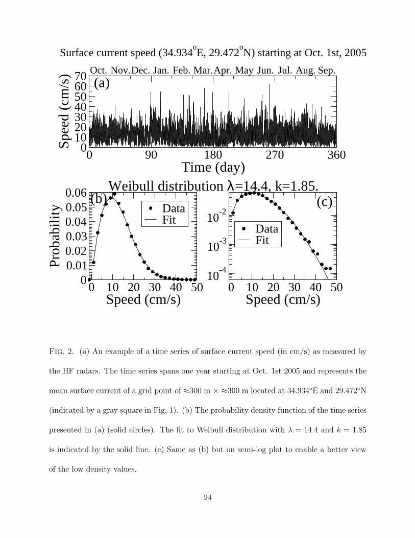
A representative example of surface current speed is shown in Fig. 2a. This current speed

time series (which spans one year) posses erratic and complex fluctuations. The distribution

of this time series is shown in Fig. 2b,c where the distribution is well fitted to the Weibull

distribution with λ = 14.4 and k = 1.85. These parameters fall in the range of parameters

reported in a recent publication (Chu 2009).

Next we derive the statistics of the distribution at each grid point and at the different

seasons (Fig. 3); half hourly data provide enough data points for such an analysis. As

mentioned above (Section 2a), the water column in the Gulf of Eilat varies significantly

between a stratified water column season (roughly between April to November) and mixed

8

water column season (roughly between December to March). This has significant effects on

the dynamics. For example, near the coast the tidal signal is strong in the stratified season

and almost absent in the mixed season (Berman et al. 2003; Monismith and Genin 2004)

. It is therefore interesting to look at the spatial and seasonal variability of the shape and

scale parameters of the Weibull distribution.

The shape parameter is clearly larger in the middle of the domain and smaller along the

periphery, both for summer and winter (left column of Fig. 3). This might be the result of

proximity to the coast which limits the cross-shore component of the velocity. The maximal

value is around 2, i.e., nearly the same as for Rayleigh distribution, but it can be as low as

1. Interestingly, the domain with maximum value shifts northward during the winter. As

for the scale parameter (middle column of Fig. 3), as expected it exhibits a similar pattern

as for the mean ocean current field (right column of Fig. 3). The results are consistent with

previous studies that indicated greater current speed during the summer; here however we

identify the location of this maximum at the southernmost (and deepest) part of the domain.

This is somehow expected as the northerly winds (and hence the wind driven component of

the currents) speedup at further distances from the northern coast of the gulf.

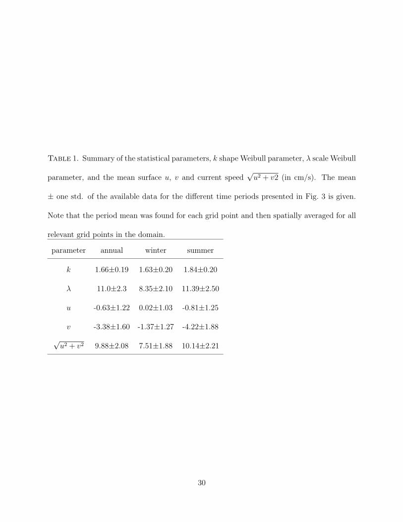
In Table 1 we summarize the results by performing a spatial mean for the fields shown

in Fig. 3 and for the zonal and meridional currents components. Here it is clear that during

summer the currents are more intense compared to the winter. In addition, the shape

parameter k is larger during the summer. The mean current direction during winter is

≈180◦ from the north in clockwise direction while during summer it is ≈191◦. However,

the mean zonal current during summer is more than three times larger than that of winter,

consistent with the more persistent currents during summer. The annual mean values are

9

closer to the summer values as the Gulf of Eilat is stratified except in winter months.

In addition to the surface currents analyzed above we also performed preliminary analysis

of deep ocean currents from the Gulf of Eilat (data from 2004 of depths of 1.5 m to 30 m,

collected close to the coast near the indicated point “1” of Fig. 1) and from the equatorial

Indian ocean (93◦E 0◦N at depth of 80 m during Oct. 2003 to Oct. 2004). It is apparent that

deep ocean current speeds also follow the Weibull distribution (with k ≈ 2 for the Indian

ocean data and k ≈ 1.3 for the Gulf of Eilat data).

We have also constructed the PDF of the zonal and meridional surface currents. With

accordance with Carlson et al. (2010) we have found that the PDF can be estimated by

exp |x − x0|α where α is between 1 and 2 (i.e., between Gaussian and exponential distribu-

tion). The PDFs were asymmetric, i.e., different α for x > x0 and x < x0.

5. A simple Ekman surface layer model

We used the model (and setting) described below in a previous study of temporal corre-

lations in the Gulf of Eilat (Ashkenazy and Gildor 2009); yet, we briefly describe the model

below for the sake of clarity.

Among the three main factors (winds, tides, and buoyancy) that affect the circulation in

the Gulf of Eilat, the winds seem to have the largest influence on surface currents. We thus

concentrate on the wind’s effect on the upper ocean layer. The classical model proposed

by Ekman (1905) was devoted to study such an effect and we use this model to study the

probability distribution of upper ocean currents.

The original model of Ekman (1905) has both time dependent and time independent

10

analytical solutions under constant winds and constant interior currents. Yet, since we are

forcing the model by the variable wind of the Gulf of Eilat (Fig. 4a), we solve the model

numerically. In particular, the following set of equations are solved:

∂u

∂t− f(v − vg) = ν

∂2u

∂z2, (4)

∂v

∂t+ f(u − ug) = ν

∂2v

∂z2, (5)

where the u and v are the zonal and meridional velocities, ug and vg are the zonal and

meridional bottom geostrophic velocities, f is the local (constant) Coriolis parameter, and

ν = 0.01 m2/s is the eddy viscosity coefficient. Here we ignore the nonlinear advection

terms, the lateral (x and y) dynamics, the basin topography, and the dependence of ν on

depth. The water density is set to be constant. At the surface the ocean is forced by the

wind through the wind stress as follows:

∂~u

∂z|z=0 =

~τ

νρo

(6)

where ρo = 1028 kg/m3 is the water density and ~τ is the wind stress vector given by

(τx, τ y) = ρaCDU(ua, va), (7)

where ua and va are the zonal and meridional wind components, U =√

u2a + v2

a is the wind

speed, and ρa = 1.3 kg/m3 is the air density. CD is the drag coefficient and is CD = 10−3 for

U ≤ 6.2 m/s and CD = (0.6094+0.063U)10−3 for U > 6.2 m/s (after Gill 1982). The Coriolis

parameter is chosen to be that of the Gulf of Eilat, i.e., f = 7.16 × 10−5 s−1. Additionally,

we chose an upper ocean layer depth of H = 50 m, a vertical resolution of ∆z = 0.5 m, and

integration time step of ∆t = 10 s. We used hourly wind data from Eilat airport during

Oct. 2005 to Sep. 2006 (Fig. 4a) to force the ocean; this time period coincides with the

11

surface currents analyzed above. The wind data was interpolated linearly to provide wind

data for the model at each time step. The interior ocean currents were modified to study

the dependence of the probability distribution on these currents.

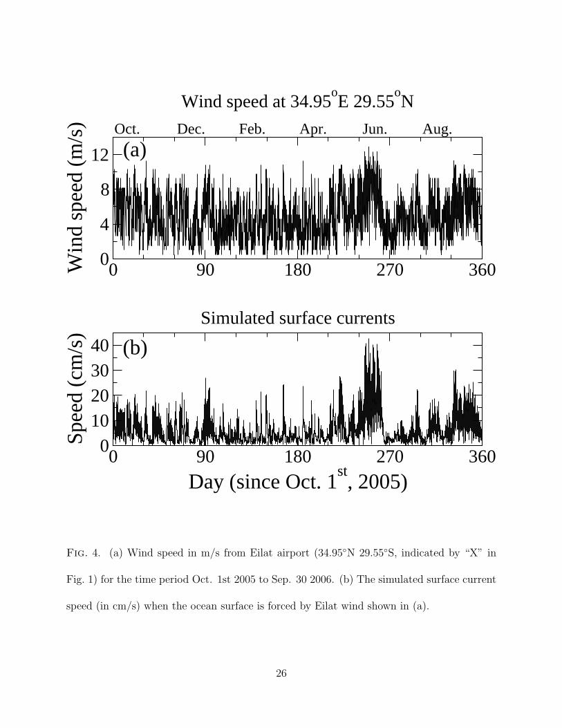
In Fig. 4 we present the Gulf of Eilat wind data used in the model and the corresponding

simulated surface current time series; in this simulation we assumed zero interior geostrophic

currents. As expected, the surface current responds nonlinearly to the wind according to

Eq. (7) and for periods where the winds were stronger, the currents were much stronger. In

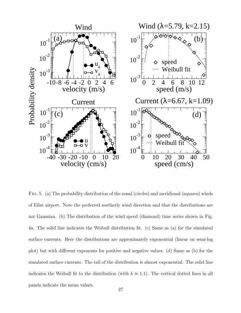
addition, the probability distribution of both the winds and surface currents are shown in

Fig. 5. Here the wind speed probability distribution seems to follow the Weibull distribution

while the currents distribution function has a stretched tail, leading to a relatively small

shape exponent, k ≈ 1.09, of the Weibull distribution; note that the Weibull distribution

with k = 1 is reduces to exponential distribution. Such a small k is inconsistent with the

observations shown in Figs. 2,3. The probability distribution of each component of the wind

and simulated current are also depicted in Fig. 5. The annual mean ± 1 std. of the zonal and

meridional wind velocities is -1.45±1.58 m/s and -4.15±3.29 m/s, indicating north-north-

eastern winds. These probability distribution functions do not follow Gaussian distribution

as is usually assumed (e.g., Chu 2009). This preferred wind direction resulted in preferred

direction of the simulated surface currents (Fig. 5); the mean ± 1 std of the simulated surface

currents are -3.17±5.71 cm/s and -1.86±5.19 cm/s such that the mean surface current vector

is oriented 40.34◦ to the right of the wind, roughly consistent with the 45◦ of the theoretical

prediction. The distribution of modeled ocean zonal and meridional surface currents is

approximately exponential (linear on semi-log curves), with different exponents for positive

and negative values.

12

The observations shown in Fig. 3 indicate that there is a spatial variability of the scale

and shape parameters of the Weibull distribution, λ and k. Since we used the Eilat surface

wind (assuming that this wind time series represents the entire domain under consideration)

we studied the model behavior under different bottom current scenarios.

When using different temporally constant bottom geostrophic currents we obtained sur-

face currents that are “riding” on the bottom currents, such that there is a minimum current

speed that is larger than zero (depending on the magnitude of the bottom speed). This re-

sulted in a probability distribution that is different than the Weibull distribution and even

different than the more generalized “shifted” Weibull distribution:

f(x; k, λ, θ) =k

λ(x − θ

λ)k−1e−(x−θ

λ)k

, (8)

for x > θ. Such distribution is inconsistent with the observations shown above and thus rule

out the possibility that the magnitude of the bottom currents underlies the spatial variability

of the parameters of the Weibull distribution.

We next assume that the bottom zonal and meridional currents are Gaussian distributed

about zero. Similar to the above, the surface water is forced by the wind of Eilat but the

noise amplitude of the bottom currents are varied. The results are shown in Fig. 6a and it

is clear that even large fluctuations of the bottom currents have little effect on the surface

current shape parameter. Moreover, the shape parameter is much smaller than the observed

ones (shown in Fig. 3). It is thus unlikely that the fluctuations of the bottom surface underlay

the spatial variability of the shape parameter of the Weibull distribution shown in Fig. 3.

Previous studies (Chu 2009) showed that when the zonal and meridional wind components

are Gaussian distributed the ocean currents are Rayleigh distributed. Motivated by this we

13

forced the model by artificially generated wind whose components are Gaussian distributed

(Fig. 6b). We estimated the k exponent for different values of amplitude of bottom current

noise (where the zonal and meridional mean current are zero) and found that the exponent

varied from ≈1.9 to ≈2. This numerical results are different from the analytical prediction

of Chu (2008, 2008) as for zero bottom currents (without noise added to them) k ≈ 1.9

while the analytical prediction was of k = 2. This difference may be attributed to the fact

that Eq. (7) was ignored in the analytical derivation of Chu (2008) or to the fact that the

analytical derivation of Chu (2008) are referred to the depth integrated (mean) currents.

As mentioned above, the surface wind data are hourly mean data and were linearly

interpolated to force the model with 10 s resolution data. Thus, wind variability (and wind

gusts) of time scale less than one hour is ignored. To mimic this variability we added

Gaussian white noise to the zonal and meridional wind components; here (Fig. 6c) the value

of the k exponent changed drastically as a function of the added noise amplitude, pointing

to fast wind temporal variability as a source for the spatial variability of the surface currents

presented in Fig. 3. The Gulf of Eilat is surrounded by high mountains that may lead to

different wind variability inside this small region. In this sense our attempts to capture the

probability distributed characteristics using a single wind time series from Eilat airport is a

simplification.

6. Summary and discussion

We analyzed the probability distribution function of surface current speed field in the

northern part of the Gulf of Eilat and found that it can be approximated by the Weibull

14

distribution. Surprisingly, we also found relatively large spatial variability of the shape and

scale parameters that characterize the Weibull distribution. These parameters were different

for summer and winter where stronger winds and larger parameters were observed during

the summer period.

We used the surface Ekman layer model to study the origin of this distribution and found

that the shape exponent of the Weibull distribution is much smaller than the observed one.

When adding Gaussian white noise to the wind field this exponent became larger, suggesting

that temporal wind gusts may be linked to the large spatial variability of this exponent.

Small-scale ocean mixing parameterization is often done using diffusion-like parameter-

izations, with an “eddy diffusivity” which is significantly larger than molecular diffusivity

(and scales with the model’s resolution), but which implies similar physical characteristics

to that of molecular diffusion. (Gildor et al. 2009) demonstrated the existence of subme-

soscale barriers to mixing, which suggest that ocean mixing is much more complex than

implied by using “eddy diffusivity”. Our present study support that conclusion: We conjec-

ture that the deviation of the distribution from a Rayleigh distribution (obtained when the

zonal and meridional components independent, uncorrelated, and Gaussian distributed) is

the manifestation of the deviation of the components from Gaussian distribution, implying

the need to find better parameterization for ocean mixing than the simple “eddy viscosity”

parameterization. Non-Gaussian distribution on the mesoscale was found before by (Bracco

et al. 2003). This also may be one of the reasons for the inability of the analyzed model

to reproduce the observed Weibull distribution and its spatial variability. In addition, the

analyzed model lacks many oceanic processes that could alter the probability distribution.

The lack of spatially varying wind field may be also a serious disadvantage of the suggested

15

model. We believe that other, more realistic models should be challenged to reproduce the

Weibull distribution of the ocean currents—preliminary analysis of general circulation model

of the Gulf of Eilat (forced by monthly mean wind) yielded distribution of surface currents

that are much different than the observed Weibull distribution.

Acknowledgments.

We thank Golan Bel and Amos Zemel for helpful discussions. This research was supported

by the Israel Science Foundation. The Eilat Port authorities gave us permission to install

one of HF radar station in the port area. Airspan provides us the wireless communication

between the radar sites. We thank the management and the staff of the Inter-University

Institute for Marine Sciences of Eilat (IUI) for their cooperation and help.

16

REFERENCES

Ashkenazy, Y. and H. Gildor, 2009: Long-range temporal correlations of ocean surface cur-

rents. J. Geophys. Res., 114, C09 009, doi:10.1029/2008JC005235.

Barrick, D. E., B. J. Lipa, and R. D. Crissman, 1985: Mapping surface currents with codar.

Sea Technology, 26 (10), 43–48.

Berman, T., N. Paldor, and S. Brenner, 2003: The seasonality of tidal circulation in the

Gulf of Elat. Isr. J. Earth. Sci., 52, 11–19.

Biton, E., J. Silverman, and H. Gildor, 2008: Observations and modeling of pulsating density

current. Geophys. Res. Lett., 35, L14 603.

Bracco, A., E. P. Chassignet, Z. D. Garraffo, and A. Provenzale, 2003: Lagrangian velocity

distributions in a high-resolution numerical simulation of the North Atlantic. J. Atmo-

spheric and Oceanic Technology, 20 (8), 1212–1220.

Carlson, D. F., E. Fredj, H. Gildor, and V. Rom-Kedar, 2010: Deducing an upper bound

to the horizontal eddy diffusivity using a stochastic Lagrangian model. Environ. Fluid.

Mech., 10 (5), 499–520.

Chu, P. C., 2008: Probability distribution function of the upper equatorial pacific current

speeds. Geophys. Res. Lett., 35, L12 606.

17

Chu, P. C., 2009: Statistical characteristics of the global surface current speeds obtained

from satellite altimetry and scatterometer data. IEEE J. of Selected Topics in Applied

Earth Observations and Remote Sensing, 2 (1), 27–32.

Ekman, V. W., 1905: On the influence of the earths rotation in ocean-currents. Arch. Math.

Astron. Phys., 2, 1–52.

Genin, A. and N. Paldor, 1998: Changes in the circulation and current spectrum near the

tip of the narrow, seasonally mixed Gulf of Elat. Isr. J. Earth. Sci., 47, 87–92.

Gildor, H., E. Fredj, J. Steinbuck, and S. Monismith, 2009: Evidence for submesoscale barri-

ers to horizontal mixing in the ocean from current measurements and aerial photographs.

J. Phys. Oceanogr., 39 (8), 1975–1983.

Gill, A. E., 1982: Atmosphere–ocean dynamics. Academic Press, London, 662 pp.

Gille, S. T. and S. G. L. Smith, 1998: Probability density functions of large-scale turbulence

in the ocean. Phys. Rev. Lett., 81 (23), 5249–5252.

Gille, S. T. and S. G. L. Smith, 2000: Velocity probability density functions from altimetry.

J. Phys. Oceanogr., 30 (1), 125–136.

Gurgel, K. W., G. Antonischki, H. H. Essen, and T. Schlick, 1999a: Wellen radar (wera):

a new ground-wave hf radar for ocean remote sensing. Coastal Engineering, 37 (3-4),

219–234.

Gurgel, K. W., H. H. Essen, and S. P. Kingsley, 1999b: High-frequency radars: physical

limitations and recent developments. Coastal Engineering, 37 (3-4), 201–218.

18

Hodgins, D. O., 1994: Remote sensing of ocean surface currents with the SeaSonde hf radar.

Spill Sci. Technol. Bull., 1 (2), 109–129.

Lekien, F. and H. Gildor, 2009: Computation and approximation of the length scales of

harmonic modes with application to the mapping of surface currents in the Gulf of Eilat.

J. Geophys. Res., 114, C06 024, doi:1029/2008JC004742.

Manasrah, R. S., F. A. Al-horani, M. Y. Rasheed, S. A. Al-rousan, and M. A. Khalaf, 2006:

Patterns of summer vertical and horizontal currents in coastal waters of the northern Gulf

of Aqaba, Red Sea. Estuarine Coastal and Shelf Science, 69 (3-4), 567–579.

Monahan, A. H., 2006: The probability distribution of sea surface wind speeds. Part I:

Theory and SeaWinds observations. J. Climate, 19, 497–520.

Monahan, A. H., 2010: The probability distribution of sea surface wind speeds: Effects of

variable surface stratification and boundary layer thickness. J. Climate, 23 (19), 5151–

5162.

Monismith, S. G. and A. Genin, 2004: Tides and sea level in the Gulf of Aqaba (Eilat). J.

Geophys. Res., 109 (C4).

Saaroni, H., E. Maza, and B. Ziv, 2004: Summer sea breeze, under suppressive synoptic

forcing, in a hyper-arid city: Eilat, israel. Climate Research, 26 (3), 213–220.

Seguro, J. V. and T. W. Lambert, 2000: Modern estimation of the parameters of the Weibull

wind speed distribution for wind energy analysis. J. Wind Engineering and Industrial

Aerodynamics, 85, 75–84.

19

List of Figures

1 (a) The flow field on Feb. 25, 2006 at 18:30 observed by two HF radar stations

(marked by “1” and “2”). The shape of the domain is nearly rectangular and

it has only one open boundary. Although the domain is only 6 km by 10 km,

there is relatively little coherence between different regions and the flow field

is rather complex. The gray square in the figure indicates the location of the

time series presented in Fig. 2a. The “X” indicates the location of the wind

speed time series presented in Fig. 4a. (b) Same as (a) for Nov. 29, 2005

11:00. Note the large scale pattern of the flow. . . . . . . . . . . . . . . . . 23

2 (a) An example of a time series of surface current speed (in cm/s) as measured

by the HF radars. The time series spans one year starting at Oct. 1st 2005

and represents the mean surface current of a grid point of ≈300 m × ≈300 m

located at 34.934◦E and 29.472◦N (indicated by a gray square in Fig. 1).

(b) The probability density function of the time series presented in (a) (solid

circles). The fit to Weibull distribution with λ = 14.4 and k = 1.85 is indicated

by the solid line. (c) Same as (b) but on semi-log plot to enable a better view

of the low density values. . . . . . . . . . . . . . . . . . . . . . . . . . . . . 24

20

3 A summary of the statistical parameters of surface current speed. The x/y-

axis denotes the longitude/latitude. The left column summarizes the Weibull

shape parameter, k, the middle column summarizes the Weibull scale param-

eter, λ, and the right column summarizes the mean current speed (in cm/s).

The top/middle/bottom panels are the parameters of the annual (Oct. 1st,

2005 to Sep. 30, 2006), winter (Jan. 1st, 2006 to Mar. 31st, 2006), and sum-

mer (Jul. 1st, 2006 to Sep. 30, 2006) time periods. The coast line is indicated

by the blue line. . . . . . . . . . . . . . . . . . . . . . . . . . . . . . . . . . 25

4 (a) Wind speed in m/s from Eilat airport (34.95◦N 29.55◦S, indicated by “X”

in Fig. 1) for the time period Oct. 1st 2005 to Sep. 30 2006. (b) The simulated

surface current speed (in cm/s) when the ocean surface is forced by Eilat wind

shown in (a). . . . . . . . . . . . . . . . . . . . . . . . . . . . . . . . . . . . 26

5 (a) The probability distribution of the zonal (circles) and meridional (squares)

winds of Eilat airport. Note the preferred northerly wind direction and that

the distributions are not Gaussian. (b) The distribution of the wind speed

(diamond) time series shown in Fig. 4a. The solid line indicates the Weibull

distribution fit. (c) Same as (a) for the simulated surface currents. Here the

distributions are approximately exponential (linear on semi-log plot) but with

different exponents for positive and negative values. (d) Same as (b) for the

simulated surface currents. The tail of the distribution is almost exponential.

The solid line indicates the Weibull fit to the distribution (with k ≈ 1.1). The

vertical dotted lines in all panels indicate the mean values. . . . . . . . . . . 27

21

6 (a) The shape parameter of the Weibull distribution, k, as a function of the

noise amplitude added to zero bottom geostrophic currents when Eilat wind

time series is used to force the ocean surface. The symbols indicate the mean

value of 30 realizations, each span one year of simulation; the error bars

indicate the standard deviation. Note the relatively small effect of the noise on

k. (b) Same as (a) but when using Gaussian distributed zonal and meridional

winds (yielding Rayleigh distributed wind speed) instead of Eilat winds. Here

k is larger and varies more drastically as a function of the noise added to the

bottom geostrophic currents. (c) Same as (a) but when using zero bottom

geostrophic currents (without any noise) but with Gaussian noise added to

the zonal and meridional wind components of Eilat winds. The added noise

drastically changes the shape parameter of the Weibull distribution. . . . . 28

22

1

1

1

11

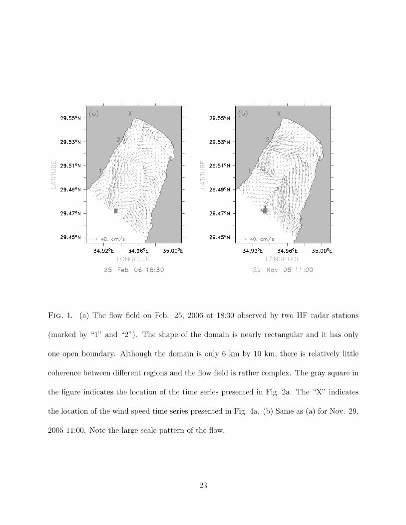
Fig. 1. (a) The flow field on Feb. 25, 2006 at 18:30 observed by two HF radar stations

(marked by “1” and “2”). The shape of the domain is nearly rectangular and it has only

one open boundary. Although the domain is only 6 km by 10 km, there is relatively little

coherence between different regions and the flow field is rather complex. The gray square in

the figure indicates the location of the time series presented in Fig. 2a. The “X” indicates

the location of the wind speed time series presented in Fig. 4a. (b) Same as (a) for Nov. 29,

2005 11:00. Note the large scale pattern of the flow.

23

0 10 20 30 40 50Speed (cm/s)

00.010.020.030.040.050.06

Prob

abili

ty

DataFit

0 90 180 270 360Time (day)

010203040506070

Spee

d (c

m/s

) Oct. Nov.Dec. Jan. Feb. Mar.Apr. May Jun. Jul. Aug. Sep.

Surface current speed (34.934oE, 29.472

oN) starting at Oct. 1st, 2005

0 10 20 30 40 50Speed (cm/s)

10-4

10-3

10-2

DataFit

Weibull distribution λ=14.4, k=1.85.

(a)

(b) (c)

Fig. 2. (a) An example of a time series of surface current speed (in cm/s) as measured by

the HF radars. The time series spans one year starting at Oct. 1st 2005 and represents the

mean surface current of a grid point of ≈300 m × ≈300 m located at 34.934◦E and 29.472◦N

(indicated by a gray square in Fig. 1). (b) The probability density function of the time series

presented in (a) (solid circles). The fit to Weibull distribution with λ = 14.4 and k = 1.85

is indicated by the solid line. (c) Same as (b) but on semi-log plot to enable a better view

of the low density values.

24

λ scale parameter − annual

Longitude

Latit

ude

(b)

34.9 34.95 35

29.46

29.48

29.5

29.52

29.54

k shape parameter − annual

Longitude

Latit

ude

(a)

34.9 34.95 35

29.46

29.48

29.5

29.52

29.54(c)

Mean speed (cm/s) − annual

Longitude

Latit

ude

34.9 34.95 35

29.46

29.48

29.5

29.52

29.54

λ scale parameter − winter

Longitude

Latit

ude

(e)

34.9 34.95 35

29.46

29.48

29.5

29.52

29.54

k shape parameter − winter

Longitude

Latit

ude

(d)

34.9 34.95 35

29.46

29.48

29.5

29.52

29.54

Mean speed (cm/s) − winter

Longitude

Latit

ude

(f)

34.9 34.95 35

29.46

29.48

29.5

29.52

29.54

λ scale parameter − summer

Longitude

Latit

ude

(h)

34.9 34.95 35

29.46

29.48

29.5

29.52

29.54

k shape parameter − summer

Longitude

Latit

ude

(g)

34.9 34.95 35

29.46

29.48

29.5

29.52

29.54

Mean speed (cm/s) − summer

Longitude

Latit

ude

(i)

34.9 34.95 35

29.46

29.48

29.5

29.52

29.54

2

4

6

8

10

12

14

2

4

6

8

10

12

14

2

4

6

8

10

12

14

2

4

6

8

10

12

14

16

2

4

6

8

10

12

14

16

2

4

6

8

10

12

14

16

1

1.2

1.4

1.6

1.8

2

1

1.2

1.4

1.6

1.8

2

1

1.2

1.4

1.6

1.8

2

Fig. 3. A summary of the statistical parameters of surface current speed. The x/y-axis

denotes the longitude/latitude. The left column summarizes the Weibull shape parameter,

k, the middle column summarizes the Weibull scale parameter, λ, and the right column

summarizes the mean current speed (in cm/s). The top/middle/bottom panels are the

parameters of the annual (Oct. 1st, 2005 to Sep. 30, 2006), winter (Jan. 1st, 2006 to Mar.

31st, 2006), and summer (Jul. 1st, 2006 to Sep. 30, 2006) time periods. The coast line is

indicated by the blue line.

25

0 90 180 270 360

Day (since Oct. 1st, 2005)

010203040

Spee

d (c

m/s

)

(a)

(b)

Simulated surface currents

0 90 180 270 3600

4

8

12

Win

d sp

eed

(m/s

) Oct. Aug.Dec. Jun.Feb. Apr.

Wind speed at 34.95oE 29.55

oN

Fig. 4. (a) Wind speed in m/s from Eilat airport (34.95◦N 29.55◦S, indicated by “X” in

Fig. 1) for the time period Oct. 1st 2005 to Sep. 30 2006. (b) The simulated surface current

speed (in cm/s) when the ocean surface is forced by Eilat wind shown in (a).

26

-10-8 -6 -4 -2 0 2 4 6velocity (m/s)

10-3

10-2

10-1

ua

va

Wind

0 2 4 6 8 10 12speed (m/s)

10-3

10-2

10-1

speedWeibull fit

Wind (λ=5.79, k=2.15)

-40 -30 -20 -10 0 10 20velocity (cm/s)

10-4

10-3

10-2

10-1

Prob

abili

ty d

ensi

ty

uv

Current

0 10 20 30 40 50speed (cm/s)

10-4

10-3

10-2

10-1

speedWeibull fit

Current (λ=6.67, k=1.09)

(c)

(a) (b)

(d)

Fig. 5. (a) The probability distribution of the zonal (circles) and meridional (squares) winds

of Eilat airport. Note the preferred northerly wind direction and that the distributions are

not Gaussian. (b) The distribution of the wind speed (diamond) time series shown in Fig.

4a. The solid line indicates the Weibull distribution fit. (c) Same as (a) for the simulated

surface currents. Here the distributions are approximately exponential (linear on semi-log

plot) but with different exponents for positive and negative values. (d) Same as (b) for the

simulated surface currents. The tail of the distribution is almost exponential. The solid line

indicates the Weibull fit to the distribution (with k ≈ 1.1). The vertical dotted lines in all

panels indicate the mean values.27

1.09

1.1

k

0 0.1 0.2 0.3 0.4 0.5 0.6Geostrophic currents noise amplitude (cm/s)

1.9

2k

0 2 4 6 8 10Wind noise amplitude (m/s)

11.21.41.61.8

2

k

(b)

(a) Eilat wind

Random wind

(c) Eilat wind plus noise

Fig. 6. (a) The shape parameter of the Weibull distribution, k, as a function of the noise

amplitude added to zero bottom geostrophic currents when Eilat wind time series is used to

force the ocean surface. The symbols indicate the mean value of 30 realizations, each span

one year of simulation; the error bars indicate the standard deviation. Note the relatively

small effect of the noise on k. (b) Same as (a) but when using Gaussian distributed zonal and

meridional winds (yielding Rayleigh distributed wind speed) instead of Eilat winds. Here k is

larger and varies more drastically as a function of the noise added to the bottom geostrophic

currents. (c) Same as (a) but when using zero bottom geostrophic currents (without any

noise) but with Gaussian noise added to the zonal and meridional wind components of Eilat

winds. The added noise drastically changes the shape parameter of the Weibull distribution.

28

List of Tables

1 Summary of the statistical parameters, k shape Weibull parameter, λ scale

Weibull parameter, and the mean surface u, v and current speed√

u2 + v2

(in cm/s). The mean ± one std. of the available data for the different time

periods presented in Fig. 3 is given. Note that the period mean was found for

each grid point and then spatially averaged for all relevant grid points in the

domain. . . . . . . . . . . . . . . . . . . . . . . . . . . . . . . . . . . . . . . 30

29

Table 1. Summary of the statistical parameters, k shape Weibull parameter, λ scale Weibull

parameter, and the mean surface u, v and current speed√

u2 + v2 (in cm/s). The mean

± one std. of the available data for the different time periods presented in Fig. 3 is given.

Note that the period mean was found for each grid point and then spatially averaged for all

relevant grid points in the domain.

parameter annual winter summer

k 1.66±0.19 1.63±0.20 1.84±0.20

λ 11.0±2.3 8.35±2.10 11.39±2.50

u -0.63±1.22 0.02±1.03 -0.81±1.25

v -3.38±1.60 -1.37±1.27 -4.22±1.88

√u2 + v2 9.88±2.08 7.51±1.88 10.14±2.21

30