ON THE RELATION BETWEEN TIME AND INTEN- SITY IN PHOTOGRAPHIC EXPOSURE* BY LOYD A. JONES AND EMERY HUSE A relation between the intensity of radiation causing a photo- chemical reaction and the magnitude of the photochemical change produced was found by Bunsen and Roscoe (1) in their classical researches. It was definitely established by them that the effect produced is proportional to the product of the intensity by the time during which the radiation is permitted to act and furthermore, that this effect is constant so long as the product of the intensity by the time is constant regardless of the absolute magnitude of these factors. In other words, if the exposure or insolation, as it was called by Bunsen and Roscoe, is represented by E, the intensity of the acting radiation by I and the time during which this radiation acts by t, the law may be stated by E= I t. According to this law, commonly referred to as the reciprocity law, it makes no difference whether I be large and t small or vice versa so long as the product is constant. For many years it was thought that this law applied rigidly to the case of light sensitive photographic materials. Scheiner (2) found in connection with the photographic photometry of stars that this relation did not hold. For instance, he found that increasing the exposure in stellar photography 2.5 times, which should be equivalent to an increase of one magnitude in star brightness, corresponded only to an increase of about :7 magnitude. These experiments, therefore, caused the validity of the reciprocity law to be questioned and a year or so later Abney (3) definitely proved by sensitometric measurements that the reciprocity law was not valid. Since that time this conclusion has been confirmed by many observers and there is no doubt that the Bunsen-Roscoe law fails to agree with experimental observations. The extent of the departure from the reciprocity law and the exact form of the function expressing the rela- tion between E, I and t is still, however, subject to discussion. Many workers in the field of photographic research have investigated this question and have arrived at different conclusions. The literature of the subject is too voluminous to permit _of a complete analysis of methods and results at this time. It will be well, however, to review briefly the more notable of the researches along this line. * Communication No. 193 from the Research Laboratory of the Eastman Kodak Company. 1079
Transcript
ON THE RELATION BETWEEN TIME AND INTEN-SITY IN PHOTOGRAPHIC EXPOSURE*
BY LOYD A. JONES AND EMERY HUSE
A relation between the intensity of radiation causing a photo-chemical reaction and the magnitude of the photochemical changeproduced was found by Bunsen and Roscoe (1) in their classicalresearches. It was definitely established by them that the effectproduced is proportional to the product of the intensity by the timeduring which the radiation is permitted to act and furthermore, thatthis effect is constant so long as the product of the intensity by thetime is constant regardless of the absolute magnitude of these factors.In other words, if the exposure or insolation, as it was called by Bunsenand Roscoe, is represented by E, the intensity of the acting radiationby I and the time during which this radiation acts by t, the law maybe stated by E= I t. According to this law, commonly referredto as the reciprocity law, it makes no difference whether I be largeand t small or vice versa so long as the product is constant. For manyyears it was thought that this law applied rigidly to the case of lightsensitive photographic materials.
Scheiner (2) found in connection with the photographic photometryof stars that this relation did not hold. For instance, he found thatincreasing the exposure in stellar photography 2.5 times, which shouldbe equivalent to an increase of one magnitude in star brightness,corresponded only to an increase of about :7 magnitude. Theseexperiments, therefore, caused the validity of the reciprocity law to bequestioned and a year or so later Abney (3) definitely proved bysensitometric measurements that the reciprocity law was not valid.
Since that time this conclusion has been confirmed by many observersand there is no doubt that the Bunsen-Roscoe law fails to agree withexperimental observations. The extent of the departure from thereciprocity law and the exact form of the function expressing the rela-tion between E, I and t is still, however, subject to discussion.
Many workers in the field of photographic research have investigatedthis question and have arrived at different conclusions. The literatureof the subject is too voluminous to permit _of a complete analysis ofmethods and results at this time. It will be well, however, to reviewbriefly the more notable of the researches along this line.
* Communication No. 193 from the Research Laboratory of the Eastman Kodak Company.
1079
[J.O.S.A. & R.S I., 7
As stated previously, Scheiner (loc cit.) working on stellar photog-
raphy obtained evidence which indicated that the reciprocity lawwas not valid and in 1893 Abney (loc. cit.) definitely verified this bysensitometric measurements. Abney concluded that the relationcould be expressed in the form E = It where p is a variable exponent.
Schwarzschild (4) and Eder (5) confirmed Abney's conclusion that thesimple relation E=I t was not valid but from their experimentalresults concluded that the facts were represented by the equationE =11P where p is a constant. This constant they found to beapproximately .86 for Schleussner gelatine emulsion plates.
A. Schellen (6) in 1898 concluded from his work that the reciprocity
law was valid and that the facts were represented by the equationE=I t.
Englisch (7) in 1901 made measurements from which he concluded
that Abney's result was correct, that is, that the exponent p must bea variable.
Sheppard and Mees (8) made some careful measurements andconcluded that the failure of the reciprocity law is not a simple functionof t and obtained measurements agreeing fairly well with those obtainedby Englisch. They further concluded that the total value of I- t doesnot influence the extent of the failure and that the failure becomesnoticeable at intensity values relatively proportional to the inertiasof the plates.
Kron (9) in 1913 carried out a very extensive research on this subjectand from his results obtained the following relation:
E~t- - Oa ( lg Is
in which a and lo are constants applying to a given emulsion butare different for different emulsions. o is termed by him the "opti-mal" intensity and is that intensity at which the blackening is amaximum for a given value of I- t. Kron's measurements have beenapplied extensively by Halm (10) to the photographic photometry ofstars and from his results it would appear that Kron's equation repre-sents the facts satisfactorily.
More recently Helmick (11) has investigated this question andhas found a very definite optimal intensity with a very marked failurefor both high and low values of I in a relatively short range of I values.He has also determined the failure using monochromatic light and haspresented equations showing the general relationship between E, Iand I. Applications of these have been made to various problems of
JONES AND HuSE1080
PHOTOGRAPHIC EXPOSURE
photographic photometry. Ross (12) has discussed the theoreticalaspect of this failure and points out the desirability of obtaining furtherreliable information in order to establish definitely the relationshipexisting between the various factors.
Work on this problem was started in this laboratory several yearsago and a large amount of fairly reliable data was obtained. It wasapparent from the values obtained at that time that the failure ofthe reciprocity law at least upon the particular materials being studiedwas much less than indicated by the results of previous observers.It was found that the equipment built for the work was not entirelysatisfactory, the chief fault being a lack of sufficient range in thevariation of I and values. These data were not published and workwas begun on a modification of the method and apparatus. A specialsensitometer was designed and constructed which was describedelsewhere (13). This instrument was completed some months ago andsince that time work has been going forward and a large amount of datawhich is thought to be extremely reliable has now been obtained. Thusfar, only three materials have been studied, these being Seed 30 plates,Seed 23 plates and motion picture (cine positive) film. The rangeof intensity and time over which observations have been made issomewhat greater than that used by previous observers. The workhas been carried out with extreme care and it is felt that the dataobtained are the most reliable thus far available:on this subject. Thevarious phases are discussed in detail in the following pages.
THE LIGHT SOURCE
The question of the most satisfactory source of radiation for usein exposing photographic materials was given very careful considera-tion. Incandescent electric lamps are by far the most satisfactoryboth in regard to quality of radiation and the precision with whichthey may be standardized and controlled. The lamps to be usedwere carefully seasoned and the voltage required for operation at acolor temperature of 2500'K. was determined by comparison withtemperature standards obtained from the Research Laboratory of theNational Electric Lamp Association. According to Forsythe (14)color temperature measurements can be made to within ±5'K. Ithas been found that the highest precision in color matching is obtainablewith the Lummer Brodhum photometer head of the contrast type.This was used in color matching the various lamps against the colortemperature standards, sets of readings being made by several differentobservers and values averaged. The lamps chosen were all of the
Dec., 1923] 1081
concentrated filament type, thus giving a source fairly small in linear
dimensions and minimizing errors due to the failure of the inverse
square law resulting from the finite dimensions of the source. Units
of 100, 250, and 500 watts were used, the higher wattages being used
for obtaining the high intensities and the 100-watt size for the low
intensities.In Table 1 are tabulated the data relative to the various lamps
used. The candle power measurements were made on a 3-meter
bench photometer using candle power standards obtained from the
National Physical Laboratory. These standards operate at approx-
imately 2500'K. and the color differences between these standards and
the lamps used in this work were practically negligible thus giving
the conditions for maximum photometric precision. Photometric
readings were made by several observers in all cases and values aver-
aged.TABLE 1
Lamp No. Watts Volts Effective Candle Power
B 250 102 72.8
A 250 110 89.4
2 100 81 1.14
4 100 85 1.03
5 100 81 1.39
6 100 79 1.40
12 500 81 131.2
7 100 79 1.40
While being measured each lamp was mounted in the lamp house
in which it was later to be used. In the case of the 100-watt lamps
which were used in a lamp house having a diffusing window which
served as the effective source of light, photometric measurements in
most cases were made on the lamp before placing it in the lamp house
as well as after.In Table 1 the values entered in the column marked "Effective
Candle Power" are those obtained with the lamp in its housing. The
greatest care was exercised in all photometric work and it is thought
that the candle power values are correct to approximately ±1%.
THE LAMP HOUSINGS
A detailed description of the sensitometer and its various parts will
be found in another paper (15). It may be well, however, to state in
[J.O.S.A. & R.S.I. 7JONES AND HuSE1082
PHOTOGRAPHIC EXPOSURE
this place the reasons for using two lamp housings of essentiallydifferent types. The distance available in constructing the instrumentwas approximately 11 meters. Assuming that the light source shouldnot be closer to the photographic material than 1 meter, a range offrom 1 to 10 meters is available for varying the intensity by the useof the inverse square law. This corresponds to a range of only 1 to100 in intensity. It was desired to vary the intensity over a rangeof approximately 1 to a million and for this a distance of 1000 meterswould be required which is obviously prohibitive. It was thereforedecided to use a lamp house carrying a diffusing window betweenthe light source and the photographic plate. The area of this diffusingsurface acting as a source can be varied to give a greater intensityrange.
It is very important, however, that nothing be introduced whichwill cause a change in the quality of the light. All available diffusingmaterial such as flashed and pot opal glass have selective transmissioncharacteristics and are therefore useless for this purpose. A diffusingelement was therefore made up using three sheets of white opticalglass fine ground on both sides. These elements were separated byapproximately 1 cm and the diffusion obtained was very satisfactory.In order to eliminate any errors due to the selectivity of this whiteoptical glass, three exactly similar sheets were mounted in the otherlamp house but without the surface grinding. The possibility of thepresence of selective scatter in the case of the fine ground surface wasconsidered and a test was made to determine if such an effect couldbe detected. Two lamps were carefully color matched against eachother on the photometer bench. One of these was then placed in thelamp house with the diffusing window and the other in the lamp housewith the clear window. The two were then placed in position on thephotometer bar and adjusted for intensity balance. No lack of colorbalance was visible. Of course, this is not a definite proof that there isno selective scatter in the region of shorter wave lengths where theeffect would have very little visual significance but a strong photo-graphic effect. However, in making the exposures overlapping at thepoint in the intensity scale where the change from the clear to thediffusing lamp house was made gave excellent agreement photo-graphically. The authors feel therefore that there is no selectivescatter occurring with the ground glass window. At least the effect isso small as to be negligible both visually and photographically.
Dec., 1923] 1083
[J.O.S.A. & R.S.I., 7
In the case of the lamp house having the diffusing window the
effective area of the surface was limited by a set of diaphragms. Thelargest of these had an aperture of 100 sq. cm decreasing by one-halffor each successive diaphragm. The effective candle power of this
lamp house was carefully determined with the various diaphragmsin position. Assuming precise cutting of the diaphragms, absoluteuniformity of illumination over the diffusing surface, and completediffusion within the effective limiting angle, candle power values shouldbe directly proportional to the specified area. The photometric meas-urements which were made with extreme care show slight departuresfrom the theoretical values. The actually measured values were usedlater in computing values of intensity. The relative candle powervalues for the diaphragms used are shown in Table 2.
TABLE 2
Lanmp House No. 2
Diaphragm Number Area Relative Candle Power
cm2
1 100.0 100.0
2 50.0 50.3
3 25.0 26.2
4 12.5 13.1
5 6.25 6.5
6 3.12 3.14
7 1.56 1.50
8 .781 .75
THE PHOTOGRAPHIC MATERIALS
There are a large number of photographic materials availablediffering in a marked degree in their sensitometric characteristics.
It is probable that the extent of the failure of the reciprocity lawis decidedly different for materials of different types. In order toobtain reliable results it is necessary in photographic research toaverage the results of a large number of observations. In this partic-ular problem many of the exposures are very long and the accumula-tion of data is a somewhat slow and laborious process. To investigatea large number of materials is therefore a great undertaking and it wasdecided to limit the initial measurements to three typical materialsand for this purpose the following were chosen: Seed 30 plates, rep-
resenting a typical high speed material, Seed 23 plates, a medium
speed material and cine positive film which has a relatively low speed.
JONES AND HuSE1084
PHOTOGRAPHIC EXPOSURE
All these are non-color-sensitive materials, that is, they are onlysensitive to the shorter wave-lengths. For the time being therefore,the complication introduced by the sensitization for the longer wave-lengths is eliminated.
Different batches of the same material may vary to a certain extentfrom each other both in speed and in contrast. It is therefore necessaryto make all measurements on a given material upon plates coated fromthe same lot of emulsion. A large quantity of each material wastherefore ordered and reserved for this work. It is well known thatthe physical condition of the plate as regards temperature and humidityhas a certain influence upon its sensitivity. In data obtained pre-viously on this subject certain discrepancies were finally traced todifferences in the humidity of the plate at the time of exposure. It istherefore considered necessary for sensitometric work of high precisionto condition the materials before exposure. For this purpose a con-ditioning box was constructed. This is so designed that the humidityand temperature are precisely controlled by automatic means. Afterthe adjustments have been made the conditions are maintained con-stant over long periods of time. The materials to be exposed in thereciprocity sensitometer were placed in this conditioning box andallowed to remain for 3 to 4 days before being exposed. It is well-known that even the most carefully manufactured plates show localvariations in sensitivity from point to point on the surface (16). Inorder to increase the precision of the data, it is necessary therefore tomultiply the number of determinations. Four sensitometric stripswere exposed simultaneously. The density readings from these fourstrips were then averaged and a final curve plotted.
DEVELOPMENT
The density produced when a photographic plate is developeddepends upon many physical and chemical factors. Among thesemay be mentioned the temperature of the developing solution, thetime of development and the chemical constitution of the developingsolution. There are other factors which influence the final density toa certain extent such as the kind of fixing bath used, the conditionsof washing and drying the plates. These latter factors, however, havea relatively small effect and the conditions can be controlled so as togive practically no density variations due to these factors.
The elimination of variation in density arising from the time andtemperature development and the constitution of the developer is
Dec., 1923] 1085
[J.O.S.A. & R.S.I., 7
more difficult. All sensitometric strips were developed in a traysurrounded by a water jacket through which water at a constanttemperature was continuously circulated. In this way variation intemperature was reduced to a minimum. The time of developmentwas also in all cases sufficiently long so that it could be determinedwith considerable precision and variations due to this cause eliminated.Great care was used in making up the developing solutions in orderto obtain an identical concentration of the various constituents.However, there seems to be a certain fluctuation in the developingpower of the organic reducing agents and batches of developer madeup at widely different times using developing agents from differentlots show lack of constancy. In the work reported in this paperexposures on the same material were developed at widely differenttimes- and while every precaution was taken to obtain a constantdegree of development, some variations occurred. In the opinion ofthe authors this is due rather to a fluctuation in the reducing powerof the developing solution than to lack of control of the physicalfactors such as time and temperature.
DENSITY MEASUREMENTS
Density measurements were made with a high intensity densitometerdescribed by one of the authors in a paper (17) on this subject. All
density measurements were made with the photographic deposit incontact with a diffusing plate. The values obtained are, therefore, ofdiffuse density. As explained in the paper dealing with the instrument,the densitometer was calibrated by application of the inverse squarelaw and it is felt that these readings are beyond criticism. Readingsobtained with this instrument have been checked also against theMartens polarization photometer which has been in use for many yearsin reading densities. This latter instrument has proven entirelysatisfactory for densities below 2.5 and within this region the twoinstruments agree to well within the photometric uncertainty.
EXPERIMENTAL PROCEDURE
The procedure for obtaining a group of strips exposed to a definite
intensity (I) for a known time (t) was as follows: The lamp housewas set in position and the distance between the source and the photo-graphic plate adjusted. From the values of distance and effectivecandle power the intensity incident upon the plate was computed.After setting the lamp house, the diaphragms for the elimination of
1086 JONES AND HuSE
PHOTOGRAPHIC EXPOSURE
scattered radiation within the housing were placed in position and thedoors in the sensitometer housing closed to exclude the room light.The gear adjustment was made to give the desired angular rotation ofthe sectored wheel. The motor was then started and brought up tospeed and checked against the standard clock. The plate-holdercontaining four strips of the material being studied was placed inposition and the dark slide drawn. The operator by manipulation ofthe light control mechanism gave the exposure. The strips were thendeveloped under standard conditions, washed and dried and the densityvalues determined. As a rule, several sets of strips exposed at thevarious values of I were available for development at the same time.It is not feasible for an operator to handle more than about twelvestrips at a single development. The group exposed together weretherefore broken up and developed with strips exposed at other inten-sities. In this way variations due to extent of development were toa certain extent smoothed out. The density values obtained from thefour strips exposed at a given intensity were averaged and the sensi-tometric curve plotted.
In Table 3 are shown the density values obtained from agroup of four Seed 30 strips exposed under an illumination of 4.55meter candles, the exposure time for the maximum step being onesecond. These values serve to illustrate the uniformity of densitythat can be expected in work of this kind. From the values obtainedby averaging the four groups of readings, the curve shown in Figure 1is plotted. This procedure was then repeated for various values ofintensity and for each intensity used a curve similar to that shownin Figure 1 was obtained. For a given material, this group of curves
Dec., 1923] 1087
[J.O.S.A. & R.S.I., 7
represents the basic data from which the relations existing betweenintensity, time, and exposure are later computed.
THE REDUCTION OF DATA
The elimination or minimization of systematic and accidental errorsin photographic work is of great importance. It is common experienceamong workers in this field that the precise duplication of results is
3.0
2.4
zlaW
1.8
1.2
.6
0.0 0.6 1.2 1.8LOG T,,,LA.
FIG. 1. Typical H and D Curve.
2.4 3.0
extremely difficult. These errors arise from many causes among whichmay be mentioned lack of absolute uniformity in the materials them-selves and lack of complete control of various factors in the develop-ment, washing, fixing, and drying of the test strips.
Where high precision is desired, it is necessary to make a largenumber of observations from which the final and most probable resultmay be computed. The most satisfactory method of reducing suchdata is not always the determination of an arithmetical mean of agroup of observed values. In some cases it is much better to smoothout variations by a graphic method. This is accomplished by plottingthe observed values, drawing the most probable smooth curve as
indicated by these points, and reading back from this smooth curve
SET 40 I - 4.55 M.C.
SEED 30 LOG TM=, 0.0
LOG TA = 0.66
- _
X I.. I
JONES AND HuSE1088
PHOTOGRAPHIC ExPOSURE
the desired numerical values. The method of reducing the originaldata obtained from the test strips has been given very careful considera-tion by the authors, and it is felt that the method finally adoptedreduces experimental errors to a minimum. Since the interpretationof photographic data is of prime importance, it is deemed advisable topresent at this time a detailed account of the way in which the originaldata were treated. For this purpose all of the data and each step inits reduction to final form for one of the materials studied will be given.
TABLE 4(Seed 23)
1 2 3 4 5 6 7 8 9 10
Set Strips Source Lamp Aper- Eff. D(m) I(mc) Tmax (mas)House ture cp Ms
DATA RELATIVE TO SEED 23In Table 4 is given a complete record of all exposure conditions
for the tests made on Seed 23 plates. The numbers in the first columnrepresent the arbitrary designation of the group of strips exposedunder identical conditions, while in the second column is shown thenumber of strips comprising that group. In -columns 3 4j and 5 arethe detailed specifications of the particular light source used, the lamphousing in which it was mounted, and in the case of the lamp house forthe low intensities, the number of the diaphragm used to control theeffective area of the source. In column 6, the numbers indicate the
Dec., 1923] 1089
[J.O.S.A. & R.S.I., 7
effective candle power of the source assembly including the lampitself, the lamp housing, and the limiting diaphragm. These valueswere determined directly on the bench photometer against reliablestandards of candle power obtained from the Bureau of Standardsand the Electrical Testing Laboratories. The utmost care was usedin the photometric work and it is thought that all values presentedare correct to within ±1%. As stated previously, all lamps werecarefully color matched against color temperature standards and it isestimated that the color temperature of the various sources is constantto within ±50. In column 7, the numbers indicate the distance inmeters-between the light source and the plane occupied by the photo-graphic plate during exposure. In the eighth column the valuesindicate the illumination in meter candles incident upon the exposureplane. In the ninth column, the values are the time of exposure forthat step of the sensitometric strips receiving the maximum exposure.As explained in the paper (15), describing the sensitometer in detail,the sensitometric strip consists of ten possible steps, the exposure timevarying by consecutive powers of 2 from step to step. For conveniencein recording results, these steps are referred to by numbers from 1 to10, 1 in all cases designating that step receiving the maximum exposure.In column 10 are tabulated the values of I-t in mcs for step No. 1 ofthe strip. It will be noted that the values in column 10 are onlyapproximately constant. This exposure was found to give a stripconsisting of nine measurable densities and amply sufficient for theestablishment of the characteristic curve. It would have been necessaryto double, approximately, the exposure in order to utilize the ten stepsavailable and this was not considered necessary.
The density of the various areas of each strip was measured andthe values for each group of strips were averaged. These values aretabulated in Table 5, the numbers at the top of each column indicatingthe corresponding step number on the strip. From these values acharacteristic H and D curve was plotted for each group, the ordinatesof these curves being density and the abscissae log exposure in m.c.s.It should be emphasized that the log E value (that is log of I- t) for thevarious densities tabulated in column 1 of Table 5 is not constant.These density values when plotted at the proper log I position producecharacteristic curves in such position that the variations in the valuesof I. t shown in column 10 of Table 4 are eliminated by reading fromthe plotted curves the density values corresponding to a constant valueof log I t.
1090 JONES AND HUSE
PHOTOGRAPHIC ExPOSURE
From the characteristic curves plotted from the various groupsof data shown in Table 5, the y for each group was determined. Thisvalue of y is an indication of the extent of development and should beconstant for all groups if we assume that y is independent of intensity.Gamma (y) values for each group are tabulated in the last column ofTable 5. An inspection of these shows that considerable variationoccurs. As was pointed out previously, several weeks elapsed between
TABLE 5
(Seed 23)
Density (for the indicatted step number on strips) _
the beginning and conclusion of this work so that several differentmixings of developer were used. The authors consider that a relativelylarge variation in y is due to unforeseen variations in the developingsolution. In Table 5, the results are arranged not in a chronologicalorder in which the exposures were made, but according to a continuouslydecreasing value of I. The results in this table show no systematicvariation of y with intensity; however, it was considered desirableto make a specific test of this fact.
For this purpose, four strips were exposed at an intensity of 131meter candles and another group of four strips at .0058 meter candles,the exposure time being adjusted so as to give-approximately equal
Dec., 1923] 1091
[J.O.S.A. & R.S.I., 7
exposure in the two cases. These eight strips were then placed in atray and developed simultaneously, and the densities read and plotted.The results are shown in Figure 2, curve A being for the group exposedat high intensity and B for that exposed at a lower intensity.
2.4SEED 23
2.0 A- 131.2 -OG.0058
1.6
I6
z
FIG. 2. Characteristic curves for different intensities.
It will be noted that there is no measurable difference in the slopeof the two curves nor is there any indication that the curves differin any way in general shape. This was repeated several times, in allsome thirty or forty strips being exposed in groups at various intensitiesand developed together. For this particular material, it was impossibleto detect any dependence of -y upon intensity. This fact being estab-lished it is necessary in some way to smooth out the y variations occur-ring in Table 5. The mean value of y for the entire group of deter-minations is .95. It is therefore necessary to correct each characteristiccurve to that y value.
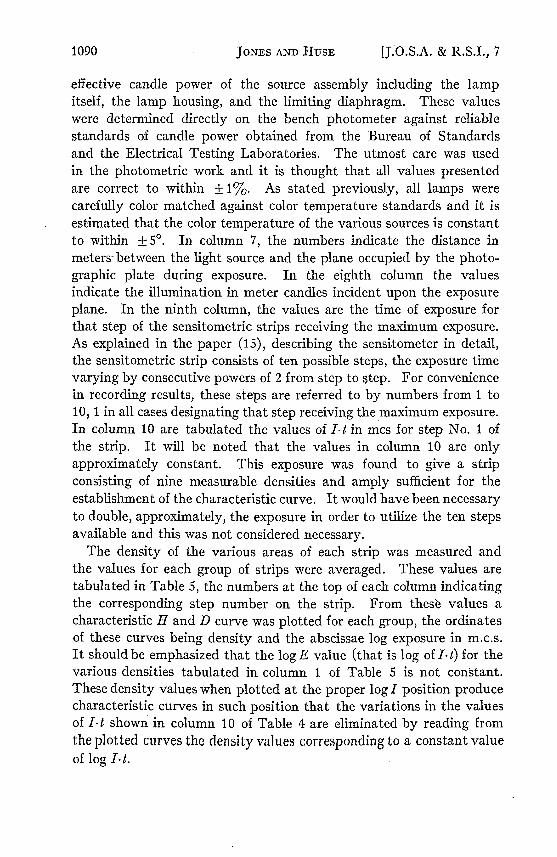
Before passing on to the method for making these corrections,it may be of interest to consider briefly Figure 3. In this figure theobserved y values are plotted as a function of log intensity. Thenumber adjacent to each point is that of the group to which the valueapplies. It will be noted that the y values of groups 51 to 58 inclusiveare practically equal. These numbers indicate the chronological orderin which the exposure was made and also indicate roughly the orderof development. These groups were probably all developed in thesame mixing of developer and show no indication of any systematic
1092 JONES AND HuSE
PHOTOGRAPHIc ExPOSURE
dependence of y upon the intensity. Groups 65 and 66 show relativelylow y but as indicated by their number they were made at anothertime and probably show the effect of inconstancy in developer. Like-wise groups Nos. 97 to 103 show relatively low -y, but they againprobably represent different mixings of developer.
SEED 23
24 _
12
° 51 ! B 100 7 e 5 96 9o
_Z __.6 _ _ _ _ _ _ _ _ _ _ _ _ _
'Ss 2.2 26 4 0.6 LOG INTENSITY
FIG. 3. Variation of gamma with intensity.
While the points, if considered entirely apart from other information,would indicate a slight decrease of y for the very low and very highintensities, the authors consider that in view of other informationand other tests there is no indication whatever of a dependency of-y upon intensity. The most probable y-intensity curve is thereforea straight line parallel to the intensity axis and having a -y value of .95.
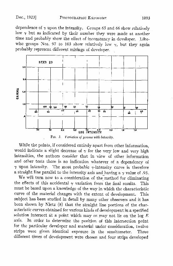
We will turn now to a consideration of the method for eliminatingthe effects of this accidental y variation from the final results. Thismust be based upon a knowledge of the way in which the characteristiccurve of the material changes with the extent of development. Thissubject has been studied in detail by many other observers and it hasbeen shown by Nietz (8) that the straight line portions of the char-acteristic curves obtained for various kinds of development in a specifiedsolution intersect at a point which may or. may not lie on the log Eaxis. In order to determine the position of this intersection pointfor the particular developer and material under consideration, twelvestrips were given identical exposure in the sensitometer. Threedifferent times of development were chosen and four strips developed
Dec., 1923] 1093
[J.O.S.A. & R.S.I., 7
for each of these times. The density values were read and averagedfor each development time. The curves obtained are shown in Figure
4. This group of curves gives an intersection point at D = -. 30.
This result was checked by several other independent sets of observa-tions.
a
I-vsz1w1a
SEED 23
:.0
.6I
.2 /
.8 ~
4
.c 1 0~6 I2 18 24 0LOG E
FIG. 4. Position of intersection point.
Having established the position of this intersection point for thematerial, we are now in position to correct the slope of each of the
characteristic curves plotted from the data tabulated in Table 5.
Referring to Figure 1, if the straight line portion be extended below
the axis and on this extension a point be located at D= -. 30 and
through this point a straight line drawn having a slope of .95 (mean
value of y from Table 5), the line so drawn will be the straight line
portion of the desired corrected characteristic curve. Using this
straight line then as a basis, the corrected curve can be reconstructed.
By proper averaging, it is possible to determine the mean shape of
the characteristic curve as established by all of the data in Table 5.
The shape and position of the toe and shoulder of the characteristiccurve were determined in this way and drawn in proper relation to thestraight line established as previously described. In Figure 5 thecurve indicated by the dotted line (A) is that plotted from the originalobservations of set 56 and the solid line curve (B) is the corrected
The corrected characteristic curve for each group of strips wasdrawn and from them the density values tabulated in Table 6 were read.The numbers at the top of each column are the values of I-t to whichthe indicated densities apply. The step number on the strip has nowbeen eliminated, and in this way the variations in the I-t value for a
[J.O.S.A. & R.S.I., 7
given step number as shown in Column 10 of Table 5 have been elimi-
nated. It will be noted that the first column in Table 6 is for an tvalue of 64; this is greater than any exposure actually given and isobtained by extending the corrected characteristic curve a shortdistance beyond the last observed point. The shape of the character-istic curve is so well established that this procedure is consideredallowable.
e --t*SEED2W~~~~~~~~~~~~~
FIG. 6. Variation of density with itensity. Each curve for a
I 0.0 1.5
constant value of I- t.
TABLE 7
Curve 1-t
A 64B 32C 16D 8E 4F 2G 1H .5I .25J .125
From the data of Table 6, the curves shown in Figure 6 were plotted.These curves represent density as a function of log I for various con-stant values of I-t. The values of the product It for the variouscurves indicated by the letters, A, B, C, etc. are shown in Table 7.In drawing these curves, a final smoothing out of the experimental
JONES AND HusE1096
Dec., 1923] PHOTOGRAPHIC EXPOSURE 1097
variations is obtained. In fact the actual points obtained from thedata in Table 6 give curves with few irregularities. However, someslight variations were observable and in drawing the curves in Figure6 the most probable position and shape was chosen. It is now possibleto read back from the curves in Figure 6 the data tabulated in Table 8.
TABLE 8(Seed 23)
Log t
Log I
mc
2.11.81.51.20.90.60.30.01.71.4
1.1
2.82. 52.23.93.63.33.04.7
Imc
27
26
26
242322
2'202-12-2
2-3
2-42-62-6
2-72-82-92-102-11
3.0
2-10
.07
2.242.091.881.681.441.17
.88
.60
.34
0.0
20
.12
2.242.101.881.651.381.06
.74
.40
3.0
_ 210
3.3
2-9
.24
.08
2.252.101.911.701.441.18
.88
.60
0.3
21
.33
.12
2.242.081.871.641.351.03
.70
3.3
211
3.6
2-8
.49
.28'.09
2.262.111.911.701.451.17.88
0.6
22
.59
.33.12
2.232.071.851.621.32
.99
3.6
212
3.9
2-7
.79
.53
.30
.to
2.262.111.921.701.451.17
0.9
23
.88
.59
.32
.11
2.222.061.831.591.28
3.9
213
2.2
2-s
1.06.81.55.31.10
2.262.121.921.701.44
1.2
24
1.16.87.58.30.10
2.212.041.811.56
4.2
214
2.5 2.8
2-5 2-4
1.34 1.601.10 1.36.83 1.12.56 .86.32 .58.10 .32
2.26 -112.12 2.261.92 2.121.70 1.92
1.5 1.8
25 26
1.44 1.701.16 1.43
.86 1.15
.56 .85.28 .54.09 .28
2-20 .08
2.02 2.181.80 2.01
4.5 4.8
215 216
1.1i
2-3
1.861.631.391.14
.87
.58.33.12
2.262.11
2.1
27
1.921.691.431.13
.83
.51
.23
.06
2.17
5.1
217
1.4
2-2
2.041.871.651.421.16
.87
.59
.34
.12
2.25
2.4
28
2.111.911.681.421.12.80.48.19.03
5.4
218
1.7
2-1
2.222.071.891.671.431.16.88.60.34.12
2.7
29
2.252.101.901.671.401.09
.78
.44
.15
5.7
219
Log t (sec.)
I (sec.)
Log I (sec.)
t (sec.)
Log I (sec.)
t (sec.)
Certain definite values of I were chosen spaced at uniform intervalsalong the log I axis, the highest being log I = 2.1 (I = 128 mc). Theinterval used was log I = 0.3 thus giving intensity values decreasingby consecutive powers of 2. These log I and I values are enteredin the first two columns of Table 8. At each log I value, densityvalues were read for each of the curves, A, B, C, etc. (Figure 6). Thedensities are tabulated in line horizontally with the correspondinglog I and I values. The values of log t and applying to each of the
[J.O.S.A. & R.S.I., 7
densities thus obtained are indicated by the figures in the columns thusdesignated. The values of log t and at the top of the table apply onlyto those densities down to and including the underscored value ineach column. Values of log and t in the middle of the table applyto those densities between the underscoring lines in each column;and those at the bottom to the densities below the underscored valuein each column. From these data now, it is possible by reading alonga horizontal line to obtain the characteristic curve determined withI constant and variable, while by reading the perpendicular columnsthe characteristic curve for t constant and I variable may be plotted.The data contained in Table 8 and the curves in Figure 6 representthe final reduction of the observations.
In case there were no failure of the reciprocity law,. the curves inFigure 6 would be horizontal lines parallel to the log intensity axis.It should be noted that there is a perceptible curvature to these lines,all being somewhat higher in the region of log I = 1.7 than at the higherand lower intensities. The departure from straight line form is not,however, very great considering the enormous range of intensityincluded. There also seems to be a distinct tendency for the curvesin the intermediate density region to show a more marked departurefrom the straight line condition than those in the low and high densityregions. While there is undoubtedly an intensity which gives a maxi-mum density for constant 1, the location of the position of thisso-called "optimal" intensity must in the case of this material at leastbe subject to great uncertainty.
DATA RELATIVE TO SEED 30
The method of reducing the data to final form for this materialis very similar to that used with the data on the Seed 23 plates. InTable No. 9 are given the original density values. Each group consistedof from 4 to 8 sensitometric strips and the values shown are the averagesfor each group. The illumination incident on the plate during ex-posure is given in the column marked log I. The mean gamma valuesfor each group are shown in the column thus designated, while in thelast column marked I t (max.) are the exposure values (in mcs) forstep No. 1 of each group. It will be noted that there is some variationin the value of gamma. There is no doubt in the author's mind thatthis variation is attributable to the developing solution. It will benoted that the groups designated by consecutive numbers show verylittle variation in the gamma values.
Specific tests were made to determine whether or not any gammavariation due to the intensity factor could be measured. In Figure 7are shown two characteristic curves, A, made with an illumination of4.3 mc and B, with an illumination of .0014 mc. Several strips were
t.
a
.
I.
SEED 30
A- I 43 M.C. A/B- I .0014M.C. _ _
.2
4 ~
. 0 0 a6 1 2 L6E1. 24 3 ,LOG E
FIG. 7. Characteristic curves for different intensities.
1100 JONES AND HUSE [J (.O.A. & 1 Y.S;.1., 7
exposed at each intensity and all strips of both groups developedsimultaneously, the densities when read and averaged gave the curvesshown. It will be noted that there is no detectable difference in theslope of the two curves. Several other direct tests of this point weremade and in no case could any definite evidence of the dependence ofgamma upon intensity be found.
It has therefore been considered allowable to average the values ofgamma shown in Table 9, and to correct all of the various group curvesto this gamma in order to smooth out density variations due to develop-ment differences.
I.-
zcloa
I.1 4.7
In Figure 8log intensity.to .83, the mea
By a metho
3.3 3.9 2.5 IT 1.7 0.3LOG INTENSITY
FIG. 8. Variation of gamma witlt intensity.
are shown the gamma values plottedThe straight horizontal line is drawn.n value from Table No. 9.d exactly similar to that used in the
0. 1.5 2.1
as a function ofat gamma equal
case of Seed 23material, the intersection point for the Seed 30 plate and the developingsolution used was determined and from a mean of five groups of stripswas found to lie at a value of D = -. 25. By extending the straightline portion of the characteristic curve below the axis of zero densityand locating on that line the point where D = -. 25 and drawingthrough the point thus established a straight line having a slope of.83, the straight line portion of the corrected characteristic curvewas established. By averaging values from the original curves themean shape of the toe and shoulder was determined and by applying
SEED3 0
'.9 ~
I.2 ~0 00
0 _ -_ _.6 ___ .
r _ rs . n Ts T A_
I
Dec., 19231 PHOTOGRAPHIC EXPOSURE 1101
these mean shapes to the established straight line portion the finalcorrected density-log E curve for each group was drawn. An exampleof this correction is shown in Figure 9.
From these corrected curves the density values tabulated in Table10 were read. Points on the log E axis were so chosen that for all thegroups density values apply to certain constant values of 1-t as indi-cated by the numbers at the top of the respective columns.
From the data in Table 10, the curves shown in Figure 10 wereplotted, these being similar in type to those shown for Seed 23 materialin Figure 7. The curvature in the case of this material is somewhatgreater than for Seed 23 but again the departure from the straightline'relationisnot great except for very low intensities. Here alsothe7locationofthe most probable value of the optimal intensity issubject touncertainty. Each curve shown represents the density fora constant value of It. The l1I value for Curve A is 64 (mcs) thevalues forthe others in the series decreasing by consecutive powersof 2. Itwill be noted that these curves fit fairly well with the pointsdetermined and this represents the final graphical smoothing out of thedata. From these curves the values tabulated in Table 11 were read andthese values represent the final conclusion relative to this material.The method of tabulating is identical with that used in Table 8 whichwas described in detail.
SEED 30
2.4
~La
LZ
U a .7 al 39 s tc 1.7 0 0.9 tus 2.1LOG INTENSITY
FIG. 10. Variation of density with ittentsity. Each; curve for a cotstant valte of I- t.
DATA RELATIVE TO MOTION PICTURE (CINE POSITIVE) FILM
The density values read from the sensitometric strips of this materialare given in Table 12 with the values of illumination, gamma, and
1 102 JONES AND HUSE
PHOTOGRAPHIC EXPOSURE
TABLE 11
(Seed 30)
Log I
mc
2.11.81.51.20.90.60.30.01.7
1.41.12.82.52.23.93.63.33.0
4.7
4.4
I
mc
27
26
25242322
21202-1
2-2
2-32-42-52-62-72-82-92-10
2-11
2-12
4.4
212
.16
2.011.821.641.411.16
.90
.65
.40
1.1
2-3
.18
2.031.821.591.331.04.76.44.17
1.8
26
05
1 .66
4.7
2-11
.38.18
2.021.831.641.411.17.90.65
1.4
2-2
.40
.17
2.021.801.561.291.00
.70
.38
2.1
2'
.13
.03
3.0
2-"0
.62
.39.18
2.031.841.641.421.16
.90
1.7
2-1
.64
.39
.16
2.001.771.521.24
.94
.64
2.4
28
.33
.09
3.3
2-9
.87
.63
.40
.18
2.041.841.651.421.16
0.0
20
.90.64.37.15
1.971.741.481.19
.89
2.7
2'
.58
.26
3.6
2-8
1.12.88.64.40.20
2.041.841.651.42
0.3
21
1.16.89.62.34.14
1.941.701.421.13
3.0
2"
.83
.51
3.9
2-7
1.361.14
.89
.64.40.21
2.041.841.65
0.6
22
1.421.15
.88
.60
.32
.12
1.901.641.36
3.3
211
1.06.77
2.2
2-
1.601.381.15
.90
.65
.41
.20
2.041.84
0.9
23
1.651.411.13
.85
.57
.28
.10
1.851.59
3.6
212
1.30.99
2.5
2-5
1.801.611.391.16
.90
.65
.41
.19
2.04
1.2
24
1.841.641.391.11
.82
.53
.25.08
1.80
3.9213
1 .531.23
2.8
2-4
2.001.811.621.401.16
.90
.65
.41
.18
1.5
25
2.041.841.611.361.08
.79.49.21.07
4.2
214
1.731.46
Log t (sec.)
(sec.)
Log t (sec.)
I (sec.)
Log t (sec.)
t (sec.)
I-t (max.) in the columns as indicated. An inspection of the gammavalues show that they are fairly constant with the exception of thevalue for Set No. 84 which was exposed at the lowest intensity. Carefultests were made to determine whether or not this decrease in gammawas due to the low intensity or to other causes. In Table 13 are giventhe results of some of these tests. Set No. 1 consisted of two groups ofstrips, one exposed at an intensity of 131 mc and the other at .35mc. These two groups were developed simultaneously, read andaveraged. The gamma values obtained were 1.05 and 1.04, thus beingequal to well within the limits of experimental error. However, whenthe intensity was reduced to .022 mc as in sets Nos. 2, 3, and 4, a
lower value of gamma was in every case obtained for the low intensity.
-
.
Dec., 19231 1103
JONES AND HUSE [J.O.S.A. & R.S.I., 7
Reducing the gamma value for the higher intensity to unity andexpressing the mean gamma value at the low intensity as a decimalof that value, a mean of .86 was obtained. This is based on some 48carefully developed sensitometric strips and considered very reliable.
Plotting the gamma values asshown in Figure 11 is obtained.log itensity axis for the great
a function of log intensity, the curveThis is a straight line parallel to the
part of its length but there appears
1104
Dec., 1923] -PHOTOGRAPHIC EXPOSURE 1105
to be no doubt that there is a definite decrease in gamma for the lowerintensities. In correcting the original curves plotted from the datashown in Table 12, it is necessary to take into consideration this
E1
CINE POSITIVE
2A I
1.2
.6
. I I I ,El .7- JJ 19 2.5 -. S 0.3 0.9 1.5 Z'
LOG INTENSITYFIG. 11. Variation of gamma with intensity.
variation of gamma with intensity. The point of intersection of thestraight line portions of curves for various times of development wasdetermined as in previous cases and the corrected curves reconstructedby drawing straight lines through the points thus located. In the case
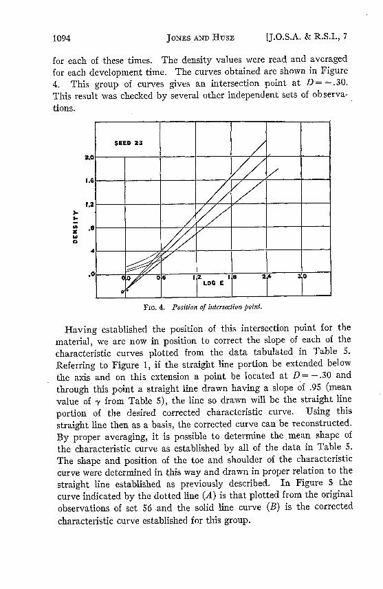
of this material, however, the slope of this straight line is not constantbut as indicated by the curve shown in Figure 11 for the variousintensities. From the corrected curves thus drawn, the values tabu-lated in Table 14 were read for certain selected values of It and fromthese values the curves in Figure 12 were plotted. The curve markedA is for I-t= 128 mcs.
From the smooth curves in Figure 12, the data tabulated in Table15 were read. These values represent to the final reduction of the datarelative to cine positive material.
The curves shown in Figure 6 (Seed 23), Figure 10 (Seed 20) andFigure 12 (cine positive) show graphically the extent of the failureof the reciprocity law for these three materials. From the data tabu-lated in Table 8, it is now possible to plot a series of H and D curves,one curve for each of the log I values shown in the column designatedas log I at the extreme left hand of Table 8. Each of these curves isfor the intensity indicated, the variation in exposure (I t) beingobtained by the variation in the value of the time factor (t). A carefulanalysis of our results shows that when one curve is plotted for each ofthe og I values shown in Table 8 a family of curves is obtained in whichthe value of gamma is constant. This particular point has receivedcareful consideration and the authors feel that there is no doubt inregard to the validity of this conclusion. This means that for thismaterial at least all characteristic curves based on a time scale willhave a constant value of gamma for designated conditions of develop-ment. If there is a failure in the reciprocity law, and the curvesshown in Figure 6 prove conclusively that there is, it follows that aseries of curves determined on the intensity scale basis must show avariation in the values of gamma, for fixed conditions of development.Since Schwarzschild's equation has been used so extensively, it seemedadvisable to determine from our data the value of the exponent pappearing in the Schwarzschild expression, E =ItP.
As pointed out by Renwick16 and Ross (c. cit.) the difference in thegamma obtained by using a time and intensity scale may be used as amethod of finding the value of the Schwarzschild constant p. Thelateral shift of the characteristic curves (plOtted for various values ofI and with t as the variable) relative to the log E scale may also beused as a means for computing p. The latter method seems to besomewhat more direct and less subject to errors arising from thegraphic determination of the gamma values. To determine the extentof the lateral shift, it was necessary to plot the characteristic curve
DeC., 1923] 1107
[J.O.S.A. & R.S.I., 7
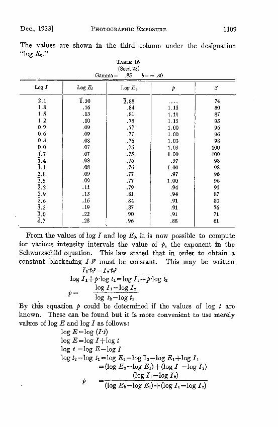
for each value of log I shown in Table 8, the density values necessaryfor this being obtained by reading the horizontal line of figures corre-sponding to the particular log I values. These curves were plottedand the straight line portion of each extended to cut the log E axis.The value of log E at the point where each curve intersects the logE axis was read and is tabulated in Table 16; in the column designatedby the heading "log Ej." In sensitometric work it is customary todesignate the value of exposure corresponding to these log E values,as the "inertia" and it is normally used as the number from which todetermine the speed or sensitivity of the material. If there were nofailure of the reciprocity law, the value of log Ei should be constant.It will be noted that this is not true. Since all of these curves havethe same gamma but different values of log E, it follows that thereciprocity failure manifests itself, when the data are treated in thisway, as a shift back and forth along the log E axis of a point at whichthe straight line extended cuts this axis. We may, therefore, use thevariation in the value of log Ei as one method of specifying the extentof the failure of the reciprocity law.
It is well known that the slope of the straight line portion of thecharacteristic curve depends upon the extent to which development iscarried. Hence the point of intersection of the straight line and thelog E axis may be dependent upon development conditions. It hasbeen shown definitely by Nietz (loc. cit.) that even in the presence ofsoluble bromides, the straight line portions of the characteristic curvesobtained with different times of development intersects in a pointwhich lies in general below the log E axis. The position of this pointof intersection is one of the most characteristic factors of the photo-graphic material and the particular developer used. A statement ofthe position of this intersection point may therefore be utilized as ameans of specifying definitely the sensitivity of an emulsion, and thevariation in the position of this point seems in this case to be the mostsatisfactory way of stating the failure of the reciprocity law.
For convenience, we will designate the point of intersection bystating the values of its co-ordinates, allowing b to represent theordinate value of the point and log E0 the abscissae value. It haspreviously been shown that for the Seed 23 plate and the developerused in this work b = -. 30. Since the gamma is constant for all of thecharacteristics curves, it is only necessary to subtract a constantvalue from the values of log E shown in Column 2 of Table 16, in6rder to obtain the desired log E values for the intersection point.
1108 JONES AND HuSE
Dec., 1923] PHOTOGRAPHIc EXPOSURE 1109
The values are shown in the third column under the designation"log Eo."
From the values of log I and log Eo, it is now possible to computefor various intensity intervals the value of p, the exponent in theSchwarzschild equation. This law stated that in order to obtain aconstant blackening I must be constant. This may be written
11-hp = I212"
log Il+p 1og tl=log I2+Plog t2log I-log 12
log 2 -log tlBy this equation p could be determined if the values of log t areknown. These can be found but it is more convenient to use merelyvalues of log E and log I as follows:
log E =log (I-t)log E=log I+log tlog t =log E-log Ilog t2-log t =log E 2-log 12-log El+log 11
Using this equation, the values of p for consecutive intervals betweenvalues of log I were computed and are shown in the column designatedas p, Table 16. It will be noted that these values range from 1.15at the high intensities down to .88 for the lowest intensities. Our data,therefore, indicate very definitely that p is not a constant as wasstated by Schwarzschild. In order to show in a different way themagnitude of the reciprocity failure, the values of sensitivity have beencomputed and tabulated in the column designated as S, Table 16.These values are obtained by taking the reciprocal of log Eo andreducing these reciprocals to relative values, assuming a sensitivity of100 at the position of optimal intensity.
TABLE 17(Seed 30)
Gamma = .83b= -.25
Log I Log Ei Log Eo P S
2.1 2.35 2.05 .... 89
1.8 .33 .03 1.07 93
1.5 .32 .02 1.03 96
1.2 .32 .02 1.00 96
0.9 .31 .01 1.03 98
0.6 .31 .01 1.00 98
0.3 .30 .00 1.03 100
0.0 .30 .00 1.00 100
1.7 .31 .01 .97 98
1.4 .31 .01 1.00 98
1.1 .32 .02 -.97 96
2.8 .34 .04 .94 91
2.5 .37 .07 .91 85
2.2 .41 .11 .88 78
3.9 .46 .16 .86 69
3.6 .51 .21 .86 62
3.3 .57 .27 .83 54
3.0 .64 .34 .81 44
4.7 .72 .42 .79 38
4.4 .80 .50 .63 32
This procedure for computing p and S was repeated with the datarelative to Seed 30 and the values obtained are shown in Table 17.Here it will be noted that the value of p is also variable, ranging from.63 at the lowest intensity up to 107 at the highest. It is of interest tonote that in the region from log I = -3.0 to -2.5 which are intensities
such as to require exposure times ranging from a few minutes to severalhours to obtain a density of unity, the mean value of p is approximately
1110
PHOTOGRAPHIc ExPOSURE
.85. These intensities represent approximately those commonly metin stellar photometry and for that particular range the value of .85 forp agrees fairly well with that found by astronomical workers. For thesame range of intensities for the Seed 23 plates, we find a somewhat
higher mean value for p. The values of sensitivity (S) show veryclearly that the failure of the reciprocity law for the Seed 30 materialis considerably greater than in the case of Seed 23 plates.
In Table 18, the values for the cine positive materials are tabulated.In this case the difference between log E, and log Eo is not constant.This follows from the variability of gamma found in the case of thismaterial. From the values of gamma shown in the last column of thetable and the value of b, it is possible to compute the difference betweenlog E; and log Eo for each particular intensity, and in this way thevalues of log Eo entered in the table were computed. From thesevalues p was computed from the equation previously given. Hereagain we find the value of p to be variable. No values greater thanunity were found but this is almost certainly because intensitiessufficiently high were not available in making exposures. The failureof the reciprocity law in the case of this material is much greater thanin the case of the other two. It will be noted that at the lowest intensitythe sensitivity is only 17% of that obtained for the optimal intensity.
Dec., 1923] 1111
[J.O.S.A. & R.S.I., 7
Had the values of log Ei (these being the values of log E where thedensity is equal to zero for each curve) been used in computing p, adifferent series of values for p would have been obtained. Likewise,had a series of log E values based on a comparison of exposuresrequired to give a constant density (for instance, D = unity) beenused, a still different series of values for p would have been obtained.Thus, if gamma is a function of intensity, p must depend upon thevalue of density chosen at which to evaluate this factor.
We have, therefore, in the case of cine positive a double variationin the value of p. All of our evidence, therefore, indicates that p cannot be constant and that the Schwarzschild expression does not expressadequately the relation between effective exposure, intensity, andtime.
Thus far, the application of other analytical expressions has notbeen made to the data in this paper.
CONCLUSIONS
From this very careful study of the failure of the reciprocity lawin the case of the three materials used, the following conclusions maybe drawn. There is a definite failure of the reciprocity law. In theSchwarzschild expression, the exponent p is not a constant. The ex-perimental determination of the value of optimal intensity must besubject to considerable uncertainty due to the extreme flatness of thecurves. For Seed 23 and 30 plates, all characteristic curves determinedon the basis of the time scale give equal gamma values when developedto the same extent, or, in other words, gamma is independent ofintensity. In the case of cine positive material, it appears to bedefinitely established that gamma is to a certain extent dependentupon intensity.
The work done thus far leaves many questions relative to thissubject unanswered and it is felt that a great deal more very carefulexperimental work is needed to solve the problem completely. Thequestion of the dependence of the failure upon the wave length of theexposing radiation is of particular interest. Further work is at thepresent time in progress at this laboratory on this subject, and it ishoped in the future to present further data which will be of useiinarriving at a satisfactory solution of this problem.
RESEARCH LABORATORY OF THE EASTMAN KODAK COMPANY,Rocms=TR, N. Y.
SEPTEMBER, 1923.
1112 JONES AND RuSE
Dec., 1923] PHOTOGRAPHIC EXPOSURE 1113
REFERENCES1. Bunsen and Roscoe. Pogg. Ann. 96. p. 96 to 373
100. p. 43 to 481" *' 101. p. 255"C " 108. p. 193
2. Scheiner, J. Application de la Photographie a la Determination des Grandeurs Stel-laires. Bull. du Comite 1, p. 227: 1889. Ast. Machr. Nr. 2889.
3. Abney, W. de W. Phot. Jour. 18 p. 302; 1893-4.4. Schwarzschild, K. Phot. Corr. 1899, p. 171. Astro. Phys. 11, p. 89, 1900. Beitrag.
zur. Phot. Photen. d Gestirne.5. Eder. Handbuch, 2, Jahrbuch, p. 457; 1899.6. Schellen, A. Inaug. Dissert Rostock, 1898.7. Englisch, E. Das Schwarzungs-gesets. Published by W. Knapp, Halle. 1901.8. Sheppard and Mees, Phot. Jour. 43, p. 48; 1903. Phot. Jour. 54; p. 282, 1914.9. Kron, Eder's Jahrbuch, p. 6; 1914.
10. Halm, J. Roy. Astronomical Soc. Monthly Notices, p. 472; June, 1922.11. Helmick, P. S., Phys. Rev. 11, p. 372; 1918.
Phys. Rev. 17, p. 135; 1921.Opt. Soc. Amer. 5, p. 336; 1921.
12. Ross, F. E., Jour. Opt. Soc., 4, p. 255; 1920.13. Jones, L. A., J. 0. S. A. & R. S. I. 7, p. 305; 1923.14. Forsythe, W. E., J. 0. S. A. & R. S. I. 6, p. 476; 1922.15. Jones, L. A. (loc. cit).16. Renwick, F. F., Phot. Jour. 40, p. 11; 1916.17. Nietz, A. H., Phot. Jour. 60, p. 280; 1920.
The Theory of Development, Eastman Kodak Co., Rochester, N. Y.
Seriengesetze der Linienspektren.-By F. Paschen and R. Gtze.ii+154 pages. Springer, Berlin, 1922.This book is indispensable to workers in atomic physics. It begins
with an account of spectral series and series formulae, treated from astrictly empirical viewpoint. Practical methods for finding series andfor calculating their limits are then discussed, and the nature of termmultiplicities is described. The next section states the main resultsof the quantum theory of spectroscopy, with applications of innerquantum numbers to the explanation of doublet and triplet con-figurations. All this material is clearly written, but is so terse as to becontained in 21 pages.
The series tables follow. The numeration of spectral terms followsthe Paschen system; this is praiseworthy because this system is sofirmly intrenched in current usage. It would be well if future editionsof Paschen-Gotze and of Fowler's Report on series were to follow anexample set in the latter author's paper on triply ionized silicon;both the principal quantum number and the usual term number weregiven in that paper.
In Paschen's tables the series run in horizontal rows. This is not soconvenient to the eye as Fowler's arrangement in columns. Fowler