IEEE TRANSACTIONS ON SYSTEMS, MAN, AND CYBERNETICS, VOL. 24.

On the Representation of Uncertain Information by Multidimensional Arrays

Prabir Bhattacharya and N. P. Mukherjee

Abstract-A multidimensional approach is introduced to the repre- sentation of uncertain information in conjunction with the Dempster- Schafer theory. A multidimensional array, called a transition array, is defined, which stores the joint probabilities of the occurrences of a set of variables taking values in different sets. Using this array, it is shown how to compute the information regarding the probability of occur- rences of the variables as certain matrix products.

I. INTRODUCTION

Representation of data by higher dimensional arrays is of signif- icant practical importance. In a large number of scientific areas we need to store data (e.g., signals, images, or statistical samples) in the form of arrays. In the classical approach, we consider two- dimensional arrays only, which are usually referred to as the con- tingency tables or simply as matrices. A number of properties of the data could be investigated in terms of the structure of the linear algebra generated by these matrices. However, we could also store data instead, in the form of multidimensional arrays. One reason for doing this lies in storing large data in a compact way (the details are explained in the Appendix). This kind of representation has been found to be useful in many applications especially in the pro- cessing of data in satellite reconnaissance photographs, medical imagery, including X-ray images, image reconstruction, seismic records, and electron micrographs [I] , [2], [4], [5]. There are ap- plications of multidimensional arrays in other areas such as the de- sign of experiments, transportation planning, and defense strategic planning [lo]. In the design of VLSI structures and architectures for parallel computers (e.g., a “Hypercube”), multidimensional arrays play a significant role (see, e.g., [7]).

The Dempster-Shafer theory [ l l ] , for belief and plausibility measures, is a well-known area in knowledge engineering which has found many practical applications, e.g., in decision estimation, evaluation of software prototypes, medical diagnosis, to name just a few. There have been significant further developments to this theory, and its relationship with the theory of approximate reason- ing and fuzzy logic, e.g., [121, [14], [15], [21], [221, [231. The applications to medical diagnostics have been investigated in a number of works, e.g., [3], [13]. It was shown that the Dempster- Shafer theory of belief can be extended to include uncertain infor- mation [ 161. Arithmetic and other operations on Dempster-Shafer structures were developed in [18]. The theory of possibilistic rea- soning was introduced in [17] to represent default knowledge based on the theory of approximate reasoning ([22]), and it was further developed in a number of papers (see e.g., [19]). The possibility- probability (P-P) granule (see a review in [ 161 ) amalgamates the Dempster-Shafer theory, the theory of approximate reasoning and probabilistic information. A particular situation which is of special interest is when the relationship between the variables is captured

Manuscript received April 10, 1992; revised February 17, 1993. This work supported in part by Grant F49626-92-JC286 of the Air Force Office of Scientific Research, and matching funds from the Center of Computer and Information Sciences, University of Nebraska-Lincoln.

P. Bhattacharya is with the Department of Computer Science and Engi- neering, and the Center for Communication and Information Sciences, University of Nebraska-Lincoln, Lincoln, NE 68588.

N. P. Mukhejee is with the School of Computer and Systems Sciences, Jawaharlal Nehru University, New Delhi 110067, India.

IEEE Log Number 9212943.

NO. 1 , JANUARY 1994 I07

by a transition array and it is shown [16] that various kinds of in- formation about the variables can be obtained by computing certain products involving the transition matrix.

The aim of this correspondence is to extend [16] to a multidi- mensional setting. A multidimensional array, called a transition array is defined, which stores the joint probabilities of the occur- rences of a set of variables taking their values in different sets. Using the transition array it is possible to compute the information regarding the probabilities of occurrences of the variables in terms of certain matrix products. The multidimensional approach thus, provides a framework to represent and analyze uncertain data in a compact way. The potential applications of our multidimensional extension would include the estimation of uncertain information in a multidimensional environment, the fuzzy relational databases, and the design of medical expert systems involving vast amounts of information with several variables.

The programming language APL (“A Programming Lan- guage”) has certain basic commands to handle multidimensional arrays which makes it a good computational environment for pro- cessing multidimensional arrays. APL compilers are commercially available running on a variety of platforms (for a background on APL, see, e.g., [9]). Codes written in APL are elegant and com- pact although sometimes difficult to read. Our notation for repre- senting multidimensional arrays has been partially motivated by the APL, but the results presented here have no other overlap with APL. Three-dimensional arrays have also been considered in [SI as incidence arrays for a combinatorial structure called “associa- tion schemes on triples.”

In Section 11, we review some background material from possi- bility theory. In Section 111, we define the transition array for mul- tidimensional arrays containing uncertain information and show how to obtain information using the transition array. The main re- sult is presented for the case of three-dimensional arrays and an Appendix provides further details on multidimensional arrays.

11. PRELIMINARIES

To make this paper self-contained, we review briefly some back- ground material (for further details see [6], [ l l ] , [16], [18], [19]). L e t X b e a f i n i t e s e t a n d l e t A : X + [0, l ] a n d B : X + [0, 11,and let E - (x) : = 1 - B ( x ) for all x in X. If Vis a variable which takes values on X, we say that

V is A

to indicate that the value of Vis known to be a member of A. Two measures have been developed to examine if V is also in B; these are called the possibility measure poss [B/A], and the certainty measure cert[B/A] which are defined as follows:

poss[B/A] = max [B(x ) A A(x)]

cert[B/A] = 1 - poss[B-/A].

x s x

We remark that poss [B/A] measures the degree of overlap of A, B , and cert [B/A] measures the degree to which B contains A. Fur- ther, if A and B are crisp sets (i.e., correspond to actual subsets of X indicated by characteristic functions), then

1 i f A n B # O

0 otherwise poss[B/A] =

1 i f A G B

cert[B/A] = 0 otherwise.

0018-9472/94$04.00 0 1994 IEEE

I08 IEEE TRANSACTIONS ON SYSTEMS, MAN, AND CYBERNETICS, VOL. 24, NO. 1. JANUARY 1994

A more general structure is the possibility-probability (P-P) granule which is defined as follows. Let 6 (X) denote the set of all subsets of a finite set X . Let m : 6(X) -+ [0, 11 such that

c m(A) = 1.

The map m is called the basic probability assignment function (bpa). If A E 6 ( X ) and m ( A ) # 0, then A is called a focal element of m . Let B : X --* [0, 11. Then Pl (B), the plausibility of B is defined as

A E B ( X )

PI (B) =

and B e l @ ) , the belief of B , is defined as

@om ( B / A i ) * m (A,)) 1

Bel(B) = ( cer t (B /Ai ) * m(A, ) ) .

If m is a basic probability assignment function (bpa) from 6 (X), then we say that

Vis m.

Such a proposition is called a possibility-probability granule (P- P-granule). A P-P-granule is a means of representing uncertain information in a convenient way and this has been studied exten- sively in [ 191, where a methodology has been developed to perform various operations on the P-P granules and implement inferential reasoning.

I

111. MULTIDIMENSIONAL REPRESENTATION

In [18], two-dimensional arrays have been used to represent the relationships between variables. We now extend this approach to multidimensional arrays. We first introduce multidimensional ar- rays but we shall present the main results for three-dimensional arrays, and it is not difficult to extend the results to higher (> 3) dimensions. The Appendix provides further material towards this direction and we leave the details to the interested reader. The ex- tension from two dimension to three dimension offers some sur- prises (see the remark at the end of this section) which are not evident in the two-dimensional case. For this reason, we think it is worthwhile to investigate, in detail, the three-dimensional case from where the main idea of the generalization to higher dimensions would follow in a natural way.

* . X nk is a structure whose entries take values which are real (or complex) numbers, the ( i l , -

Dejnition: A multidimensional array A of size n, X n2 X

* , i k ) entry of A is denoted by

for all 1 5 i , 5 n,, ( r = 1, . . . , k) . We call k the “dimension” of the array (k L 1).

In the above definition, the case k = 2 corresponds to the two- dimensional arrays, Le., matrices. The case k = 3 is of special interest as it is different from the usual matrices and we can also easily visualize the three-dimensional arrays. For k > 3, no visu- alization is possible but the mathematical representation of the en- tries given by (1) remains valid.

Definition: Given an nl X * * * X nk array A and any permuta- tion u of the set { 1, . . . , k}, let A” denote the X * * * X no(k) array whose ( i , , * * , i k ) entry is given by

(A)i6!] . i o (k )

The array A‘ is called a transpose of A . The array A is called sym- metric if A“ = A for all permutations u of { 1, * . . , k} .

(For example, if u is the permutation of (1, 2, 3) which inter- changes 1 and 2 and keeps 3 fixed and A is a 3 X 3 X 3 array, then

A“ is the 3 X 3 x 3 array such that, (A‘)123 = (A)213, etc.) When k = 2, there is only one (nontrivial) transpose possible which is obtained by the interchange of the rows and columns of the matrix, and for a general k there are (k! - 1) nontrivial transposes of A . We now introduce the notation for the subarrays of a three-dimen- sional array (the corresponding notation for a higher dimensional array is given in the Appendix).

Notation: Given an arbitrary m X n X q array A , if s , t , r are fixed integers, 1 I s I m , 1 5 t I n , 1 I r I q, let A, . denote the n X q matrix whose any ( j , k) entry is and let A denote the m X n matrix whose any ( i , j ) entry is (A),,,. Then X q matrices A, , 1 I s I m represent the m vertical plane sections of the three-dimensional array A . (This also gives a convenient method to list the elements of the three-dimensional array.)

To illustrate our notation, consider the following straightforward example.

Example 1 : Let A be a 3 x 3 X 3 array whose entries are listed completely by specifying the three vertical sections given by

0.2 0.3 0.6

0.5 0.3 0.4

0.6 0.7 0.1

0.2 0.3 0.9

0.1 0.2 0.4

0.4 0.2 0.7

Then, we have, for example, the top vertical layer of A is given by

Definition. Transition Array. Let U, be certain variables taking values in the sets

x, = {Xy, . L . , x i?} (1 5 i I k)

where the n,’s are positive integers. Let T be an n l X . . * nk array such that

(T) , , lk = p r [ U I is x!:), * . . , U, is x::)] (2)

where p r denotes the probability (in the usual sense). The array T is called the transition array of the variables U, (1 I i I k ) .

The above definition is a generalization to higher dimensions of the transition matrix which was investigated extensively in [ 161. Our objective is to show that the transition array of any set of var- iables can be conveniently used to extract various kinds of expres- sions of uncertainties regarding the given variables. Since for any permutation u of { 1, . . . , k } ,

p r [ U l is xl,k), ~2 is x:,k,”, - * , uk is xIt)l

= p r [ U 2 is x!:-!’), U, is xQ’, * * , U, is XI?]. Proposition: The transition array of a set of variables is sym-

metric. We now consider some further properties of the transition ma-

trix. The treatment in the rest of this section will be restricted to three-dimensional arrays.

Notation: For the three-dimensional case, we shall use the fol-

IEEE TRANSACTIONS ON SYSTEMS, MAN. AND CYBERNETICS, VOL. 24, NO. I , JANUARY 1994 109

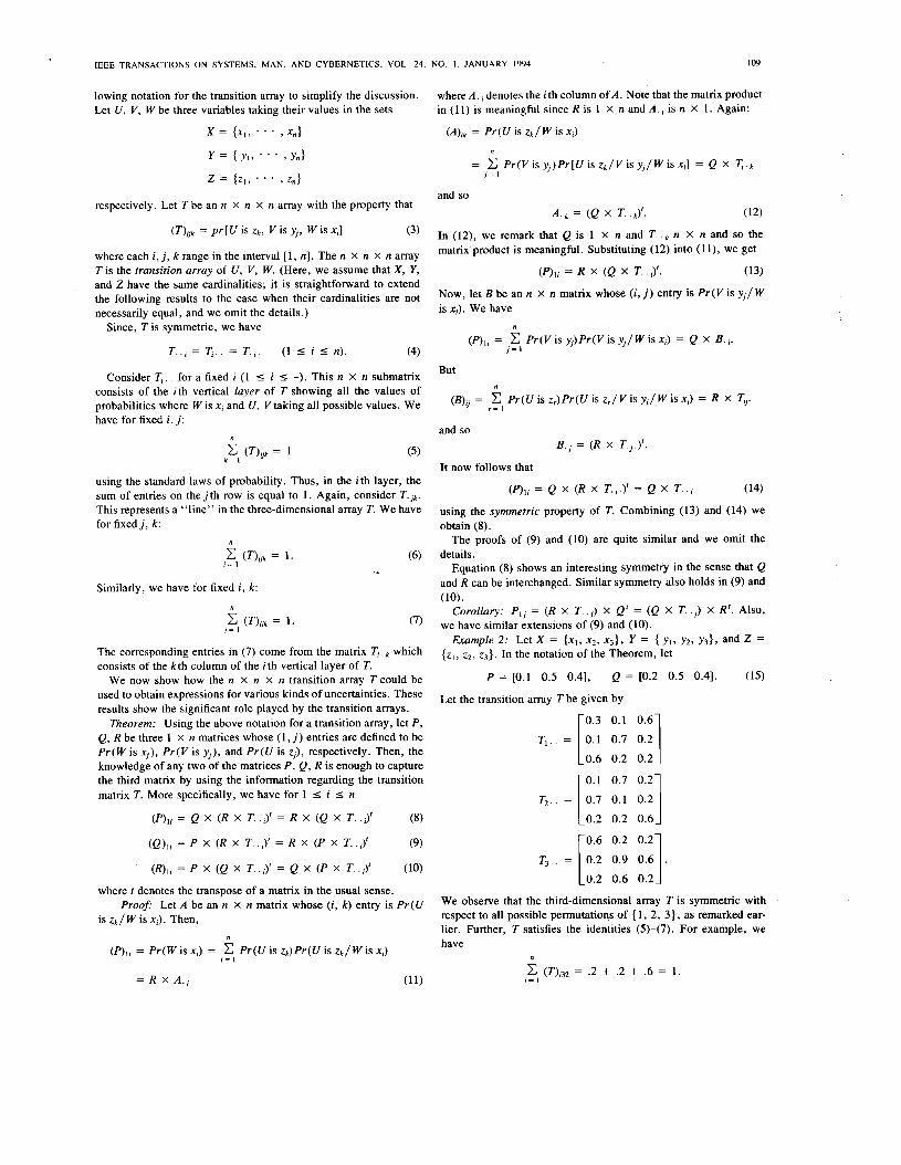
lowing notation for the transition array to simplify the discussion. Let U , V , W be three variables taking their values in the sets

where A , , denotes the i th column of A. Note that the matrix product in (11) is meaningful since R is 1 x n and A . , is n X 1 . Again:

x = {XI , * . . , X J (A)rk = Pr(U is z k / W is x,)

respectively. Let T be an n x n x n array with the property that

(T)jjk = p r [ U is Zk, Vis yj, W is xi] (3)

where each i, j, k range in the interval [ l , n]. The n X n X n array T is the transition array of U , V, W. (Here, we assume that X, Y, and Z have the same cardinalities; it is straightforward to extend the following results to the case when their cardinalities are not necessarily equal, and we omit the details.)

Since, T i s symmetric, we have

T . . ; = T i . . = T . ; . (1 I i I n). (4)

n

= P r ( V i ~ y ~ ) P r [ U i s ~ ~ / V i s y ~ / W i s x ; ] = Q x q . k j = I

and so A.k = (Q X T. .k)'. (12)

In (12), we remark that Q is 1 x n and T. .k n X n and so the matrix product is meaningful. Substituting (12) into ( l l ) , we get

(P),; = R X (Q X T . . J'. (13)

Now, let B be an n x n matrix whose (i, j ) entry is P r (V is y j / W is xi). We have

" (P),; = J = ,e I P r ( V i s y j ) P r ( V i s y j / W i s x i ) = Q x B. i .

But Consider T i . , for a fixed i (1 I i I -). This n X n submatrix consists of the ith vertical layer of T showing all the values of probabilities where W is xi and U , V taking all possible values. We have for fixed i , j :

n c (T)Uk = 1 k = I

using the standard laws of probability. Thus, in the ith layer, the sum of entries on the j t h row is equal to 1 . Again, consider T.Jk. This represents a "line" in the three-dimensional array T. We have for fixed j , k:

n

(T)jjk = 1 . (6) ;= 1 -

Similarly, we have for fixed i , k:

c (T)jjk = 1 . (7) j = 1

The corresponding entries in (7) come from the matrix T i . k which consists of the kth column of the i th vertical layer of T.

We now show how the n X n x n transition array T could be used to obtain expressions for various kinds of uncertainties. These results show the significant role played by the transition arrays.

Theorem: Using the above notation for a transition array, let P, Q, R be three 1 X n matrices whose (1, j ) entries are defined to be Pr(W is xj), Pr(V is y j ) , and Pr(U is zj), respectively. Then, the knowledge of any two of the matrices P, Q, R is enough to capture the third matrix by using the information regarding the transition matrix T. More specifically, we have for 1 5 i I n

(P) , ; = Q x (R X T. . J' = R X (Q X T . .J'

(e),; = P X ( R X T. .;)' = R X ( P X T.

(8)

(9)

(R),; = P X (Q X T. .;)' = Q X ( P X T. .J' (10)

and so = (R x T.j.)r.

It now follows that

(P),; = Q X ( R X T,; . ) ' = Q X T..j (14)

using the symmetric property of T. Combining (13) and (14) we obtain (8).

The proofs of (9) and (10) are quite similar and we omit the details.

Equation (8) shows an interesting symmetry in the sense that Q and R can be interchanged. Similar symmetry also holds in (9) and

Corollary: P l j = (R x T. . j ) X Q' = (Q X T. . j ) X R'. Also,

Example 2: Let X = {xl, x2, x3}, Y = { y , , y 2 , y 3 } . and 2 =

(10).

we have similar extensions of (9) and (10).

{z1, z2 , ~ 3 } . In the notation of the Theorem, let

P = [0.1 0.5 0.41, Q = [0.2 0.5 0.41. (15)

Let the transition array T be given by

0.3 0.1 0.6

0.6 0.2 0 .2

0.1 0.7 0.2

0.2 0.2 0.6

0.6 0 .2 0.2 I 1 0.2 0.6 0.2

T 3 , . = 0.2 0.9 0.6 . L -

where t denotes the transpose of a matrix in the usual sense.

is Zk/W is x,). Then, proofi Let A be an matrix whose (i, k ) entry is pr(u We observe that the third-dimensional array T is symmetric with

respect to all possible permutations of { 1, 2, 3}, as remarked ear- lier. Further, T satisfies the identities (5)-(7). For example, we have

n

( P ) ~ , = Pr(W is x,) = Pr(U is Zk)Pr(U is zk /w is x,) I = I n . .

= R X A , ; (T)i32 = .2 + .2 + .6 = 1 .

; = I

IEEE TRANSACTIONS ON SYSTEMS, MAN, AND CYBERNETICS, VOL. 24, NO. I , JANUARY 1994 I10

We now compute the matrix R from P , Q , and Tusing (IO). We have

@ ) I ! = P X (Q X T‘ I )

0 .3 0.1 0.6

= [ . I .5 .4] X [[O.l 0.7 0 . 2 1 )

= 0.376.

0.6 0 .2 0 .2

By computing (R)22, (R)33 in a similar manner using (IO), we get

R = [.376 0.28 0.3441. (16)

Notice that in (16), the sum of the entries of R is equal to 1, as

We observe that if we had used the second of the identities in is expected, since they represent probabilities.

( IO), namely,

@ ) i f = Q X ( P X T J‘ then the value of R which we get, is the same as the one obtained in (16). Now, we use the value of R obtained in (16), together with the given values of P and T to calculate the matrix Q , using (9). We get (after some calculations) that

Q = [0.32608 0.34528 0.328641. (17)

Notice that in (17), the sum of all the entries is, as expected, equal to 1. Comparing the value of Q given by (17) with the value of Q given by (15), we observe that they are not equal. Thus, the above analysis shows an interesting phenomenon, namely, that the rela- tionship between thematrices P , Q , R is nonlinear.

Remark: Given P and R , the value of Q, which can be computed from (9) and the transition array T, is not necessarily such that it together with P (respectively R ) would yield again the given value of R (respectively P ) when we use the corresponding equation in the statement of the Theorem.

IV. CONCLUSION

Multidimensional arrays have extensive practical applications in a large number of other areas. However, to our knowledge, no work has been done so far to develop the Dempster-Shafer theory in a multidimensional setting. Here, we have initiated such a study and shown how to manipulate uncertain information using a mul- tidimensional array, called the transition array. It is hoped that this paper will stimulate further research on multidimensional process- ing of uncertain information.

APPENDIX

In this Appendix, we give some further details for multidimen- sional arrays. The notation may appear at first to be complicated, but the generalization is conceptually not difficult. In this setting, it is possible to extend the Theorem and the Corollary proved ear- lier and we leave the details to the interested reader.

For the subarrays of a multidimensional array, we use a notation which is different when reduced to dimension 3, from the notation used in Section 11; our previous notation is not suitable for a gen- eral value of k (but fork = 3 it is very convenient). The idea behind the definition of a subarray of a multidimensional array is to “freeze” certain “coordinates” and assign them prescribed val- ues-the “dimension” of the resulting structure is equal to the number of remaining coordinates. The formal definition is some-

what complicated and so, we first describe a special case in order that the reader can see the main idea more easily.

Definition: Let A be an nl X . . . X nk array. Choose any in- tegers r a n d s, such that 1 < r < k and 1 < s, < n,. Then As, is the nl X * * - X n, - l X n,,, X . . . X nk (sub)array whose ( i l , . . . , 1,- z,+ . , i k ) entry is

. .

(A)il . . i , - Is,ir+ I . . . it

forall 1 I i , I n,, ( r = 1, In the above Definition, notice that only one coordinate of the

array A was “frozen,” and now we give a general definition where more than one coordinate may be “frozen” to generate a subarray.

Definition: Let A be an n1 X * * . X nk array. Choose a disjoint union of subsets of { 1, . . . , k } , denoted by

. * , r - 1, r + 1, * * , k ) .

where r l < * * < r, and u I I . . * I up (here, the r ’ s (and u’s ) are not necessarily consecutive elements of { I , . . . , k } ) . For each rx E R , select an integer s, such that 1 I s, < n,. Then,

As,I ’ ’ ’ s,,

is the nul X . . . X nup (sub)array whose entries are defined as follows.

Any (jl , . . * , j , ) entry where 1 I j, I nu,, (1 < p I p , up E U ) , is, (A) i , . . . ik [as defined in (I)] where each i l ( l I 1 < k ) is given by :

if 1 E R , say, 1 = rx

if 1 E U, say, 1 = up.

Notice that in the above Definition, we “freeze” those coordinates which lie in R and we let these assume the preselected values s,’s. Further, in (18) the values of the “frozen” coordinates are being displayed by the suffixes. Clearly, the “dimension” of the (sub)array given by (18) is equal to the cardinality of the set U.

Example 3: If A is an nl X . * . X nk array, then we have that A,, is an n2 X - x nk array for all 1 I s1 < nl such that [using the notation of ( I ) ]

. ’ Ik = (A)Sl . . ’ It’

Again, A,,, is an n3 X *

that * X nk array for all 1 I s2 < n2 such

( A S 1 S 2 ) 1 3 . ’ ’ Ik = ( A ) S ~ S 2 1 3 ’ ’ ’ ik.

Proceeding in this way, we get the array A,, . . . , s k - 2 which is an nk - I

x nk array (i.e., a matrix) for all 1 I s k - 2 < n k - 2 . Finally, we have the array A,, . , . s t - , which is a one-dimensional array such that

’ . ‘ S k - I), = ( A ) S l . ’ . S t - I J

for all 1 < j < nk. Using this definition of a subarray of a multidimensional array,

it is straightforward to generalize (5)-(7), which were given for the case of three-dimensional arrays. Further, the Theorem and its Corollary can be extended to arbitrary dimensions. We omit the details.

Embedding Process: From Example 3, it is easy to see that a multidimensional array can be used to “pack” families of arrays of lower dimensions in a convenient manner. For example, by ranging sk - in 1 5 sk - < nk - 2, we get a family of nk - arrays, each denoted by A s l , , . , , s k - 2 for different values of S k - 2 , each of size nk- I X nk; this entire family is embedded in the subarray

IEEE TRANSACTIONS ON SYSTEMS, MAN, AND CYBERNETICS, VOL. 24, NO. I , JANUARY 1994 I l l

As,*. . . , s k - 3 which has dimension one higher that the dimension of each member of the family. Again, by ranging S k - 3 in 1 5 s k - 3

5 nk-3, we get a family of subarrays which are embedded in As,,. . . , S t - 4 , and so on. Thus, if 5 denotes the relation of embed- ding, we have

for any choice of s,, * . , sk in the appropriate range. For the case k = 3, this embedding process can be visualized more easily (see Example I).

REFERENCES

[l] R. E. Blahut, Fast Algorithms for Digital Signal Processing. Read- ing, MA: Addison-Wesley, 1985.

[2] D. F. Elliott and K. R. Rao, Fast Transforms: Algorithms, Analyses, Applications. Orlando, FL: Academic, 1982.

[3] A. M. van Ginneken and A. W. M. Smeulders, “An analysis of five strategies for reasoning in uncertainties and their suitability for pa- thology,” in Pattern Recognition and Artificial Intelligence, E. S . Gelsema and L. N. Kanal, Ed. Amsterdam, The Netherlands: El- sevier, pp. 367-379. A. C. Kak and M. Slaney, Principles of Computerized Imaging. New York: IEEE Press, 1988. S. C. Kak, “Multilayered array computing,” Info. Sci., vol. 45, pp.

G. I. Klir and T. A. Folger, Fuzzy Sets, Uncertainty and Information. Englewood Cliffs: Prentice Hall, 1988. F. T. Leighton, Introduction to Parallel Algorithms and Architec- tures: Arrays, Trees, Hypercubes. San Mateo, CA: Morgan Kauf- man, 1992. D. M. Mesner and P. Bhattacharya, “Association schemes on triples and a temary algebra,” J. Combinat. Theory, vol. 55, pp. 204-234, 1990. R. P. Polvika and S. Pakin, APL: The Language and Its Usage. En- glewood Cliffs, NJ: Prentice-Hall, 1975. T. E. S . Raghavan, “On pairs of multidimensional matrices and their applications,” in Linear Algebra and Its Role in System Theory, R. A. Brualdi et a l . , Eds., Amer. Math. SOC., pp. 339-354, 1984. G. Shafer, A Mathematical Theory of Evidence. Princeton, Nl: Princeton University Press, 1976. - , “Belief functions and parametric models,” J. Roy. Statist. Soc.,

E. H. Shortliffe and B. G. Buchanan, “A model of inexact reasoning in medicine,” Math. Biosci., vol. 23, pp. 351-379, 1975. P. Smets, “The degree of belief in fuzzy event,” Inform. Sci., vol.

- , “The combination of evidence in the transferable belief models,” IEEE Trans. Pattern Anal. Machine Intell., vol. 12, pp.

R. Y. Yager, “Arithmetic and other operations on Dempster-Shafer structures,” Internat. J . Man-Machine Studies, vol. 25, pp. 357-366, 1986. - , “Using approximate reasoning to represent default knowl- edge,” Arti. Intell., vol. 31, pp. 99-112, 1987. - , “On the representation of transition matrices by possibility- probability granules,” IEEE Trans. Syst . , Man, Cybern., vol. SMC-

- , “On the representation of common sense knowledge by possi- bilistic reasoning,” Internat. J. Man-Machine Studies, vol. 31, pp.

347-365, 1988.

VOI. B44, pp. 332-352, 1982.

25, pp. 1-19, 1981.

447-458, 1990.

17, pp. 851-857, 1987.

587-610, 1989. [20] -, “On a generalization of variable precision logic,” IEEE Trans.

Syst. Man Cybern., vol. 20, pp. 248-252, 1990. [21] L. A. Zadeh, “Fuzzy sets as a basis for a theory of possibility,”

Fuzzy Sets & Syst., vol. 1, pp. 3-78, 1978. [22] -, “A theory of approximate reasoning,” in Selecred Papers of L.

A. Zadeh on Fuzzy Sets and Related Topics, R. Yager, S . Ovchinni- kov, R. Tong, and H. Nguyen, Eds. New York: Wiley, 1987.

[23] -, “Fuzzy logic,” Computer Mag., vol. 21, pp. 83-93, 1988.

The Fringe Distance Measure: An Easily Calculated Image Distance Measure with Recognition Results

Comparable to Gaussian Blurring

R. L. Brown

Abstract-A fast simple distance measure for calculating the degree of dissimilarity between binary images is presented. The new distance measure, called the fringe distance, gives the same degree of distortion tolerance as optimized Gaussian blurring, but can be calculated much more rapidly. Template matching using the fringe distance executes about six times as fast as Gaussian blurring template matching on an IBM AT with coprocessor, and more than three times as fast on a SUN SPARCStation I with floating point accelerator. The greater speed means more templates can be used in process time limited applications, increasing recognition accuracy.

I. INTRODUCTION

When identifying images using template matching, one com- pares the image to each of a large set of templates. The template most similar to the image is considered the correct identification. The method used to calculate the dissimilarity, or distance, be- tween the image and each template is of crucial importance. The calculated dissimilarity, or distance, between an image and a tem- plate which are identical except for small differences in size, po- sition, or proportion should be small. The image distance measure must be tolerant of small distortions or displacements of one image relative to the other [ 11, [2].

It is also crucial that the distance measure can be calculated rap- idly. For most applications, each image will have to be compared to a large number of templates, and each comparison will involve a large number of pixels. In many applications, the number of tem- plates that can be used is limited by the time needed for the com- parisons. The faster the image distance can be calculated, the more templates can be used. Using a larger number of templates will generally result in more reliable identifications.

One of the most successful methods of calculating the distance between two images has been to blur both images and then compare the blurred images pixel by pixel, calculating the sum of the squares of the differences of the blurred images at all pixels [l]. The pre- liminary blurring hides the effects of small changes in position, size, or proportion. The image may be blurred by convolving it with a Gaussian [I], [3]-[5]. It has been argued that convolution with a Gaussian is the optimal method of blumng [ 13, [6], [71.

Gaussian blurring has at least two weaknesses as a tool for tem- plate matching. First, resolution is lost by blurring. One must blur the images enough to cover small distortions and displacements without blurring them so much that there is no longer adequate resolution for making needed distinctions. The blurring parameter must be carefully chosen as a compromise between these two re- quirements. Second, calculating image distance by Gaussian blur- ring is computationally expensive. The blurring requires a convo- lution, and uses either floating point or large integer arithmetic. The subsequent distance calculation requires a subtraction, a table look up or squaring, and an addition for each pixel; all with floating point or larger integer arithmetic.

Manuscript received February 7, 1992; revised March 5, 1993. The author is with the Department of Electrical Engineering, University

IEEE Log Number 92 12942. of Arkansas, Fayetteville, AR 72701.

0018-9472/94$04.00 0 1994 IEEE