On the Sharp Stability of Critical Points of the Sobolev ...

ON THE SHARP STABILITY OF CRITICAL POINTS

OF THE SOBOLEV INEQUALITY

A. FIGALLI AND F. GLAUDO

Abstract. Given n ≥ 3, consider the critical elliptic equation ∆u + u2∗−1 = 0 in Rn with u > 0.This equation corresponds to the Euler-Lagrange equation induced by the Sobolev embedding H1(Rn) ↪→L2∗(Rn), and it is well-known that the solutions are uniquely characterized and are given by the so-called“Talenti bubbles”. In addition, thanks to a fundamental result by Struwe [Str84], this statement is “stable

up to bubbling”: if u : Rn → (0, ∞) almost solves ∆u + u2∗−1 = 0 then u is (nonquantitatively) closein the H1(Rn)-norm to a sum of weakly-interacting Talenti bubbles. More precisely, if δ(u) denotes theH1(Rn)-distance of u from the manifold of sums of Talenti bubbles, Struwe proved that δ(u) → 0 as

‖∆u+ u2∗−1‖H−1 → 0.In this paper we investigate the validity of a sharp quantitative version of the stability for critical points:

more precisely, we ask whether under a bound on the energy ‖∇u‖L2 (that controls the number of bubbles)it holds

δ(u) . ‖∆u+ u2∗−1‖H−1 .

A recent paper by the first author together with Ciraolo and Maggi [CFM17] shows that the above resultis true if u is close to only one bubble. Here we prove, to our surprise, that whenever there are at leasttwo bubbles then the estimate above is true for 3 ≤ n ≤ 5 while it is false for n ≥ 6. To our knowledge,this is the first situation where quantitative stability estimates depend so strikingly on the dimension ofthe space, changing completely behavior for some particular value of the dimension n.

Contents

1. Introduction 21.1. Main results 31.2. Comments and remarks 41.3. Analogies with the isoperimetric inequality and Alexandrov’s Theorem 41.4. Structure of the paper 52. Notation and preliminaries 62.1. Symmetries of the problem 7

2.2. Properties and spectrum of(−∆w

)−17

3. Sharp stability in dimension 3 ≤ n ≤ 5 73.1. Main Theorem 83.2. Consequences of the main theorem 113.3. The two missing estimates 123.4. Localization of a family of bubbles 123.5. Spectral Inequality 143.6. Interaction integral estimate 164. Counterexample in dimension n ≥ 6 184.1. Notation and definitions for the counterexample 204.2. First observations 214.3. The subspaces E and F are very close 224.4. The norm of ρ is asymptotically larger than ||∆u+ u|u|p−1||L(2∗)′ 244.5. The function u is a real counterexample 264.6. Construction of a nonnegative counterexample 285. Application to convergence to equilibrium for a fast diffusion equation 29Appendix A. Spectral properties of the weighted Laplacian 33A.1. Results valid for any w ∈ L

n2 (Rn) 33

A.2. Further results when w ≈ (1 + |x|)−4 35Appendix B. Integrals involving two Talenti bubbles 37References 41

1

A. Figalli and F. Glaudo

1. Introduction

The Sobolev inequality with exponent 2 states that, for any n ≥ 3 and any u ∈ H1(Rn), it holds

S‖u‖L2∗ ≤ ‖∇u‖L2 , (1.1)

where 2∗ = 2nn−2 and S = S(n) is a dimensional constant. In this paper we denote by H1(Rn) the closure

of C∞c (Rn) with respect to the norm ‖∇u‖L2 . Also, whenever a norm is computed on the whole Rn, wedo not specify the domain (so, for instance, ‖·‖L2 = ‖·‖L2(Rn)).

The optimal value of the constant S is known and so are the optimizers of the Sobolev inequality (see[Aub76; Tal76]): the functions that satisfy the equality in (1.1) have the form

c

(1 + λ2|x− z|2)n−22

,

where c ∈ R, λ ∈ (0, ∞), and z ∈ Rn can be chosen arbitrarily. Let us define a subclass of all theoptimizers, that is the parametrized family of functions U [z, λ], with z ∈ Rn and λ > 0, defined as

U [z, λ](x) := (n(n− 2))n−24 λ

n−22

1

(1 + λ2|x− z|2)n−22

. (1.2)

We will call such functions Talenti bubbles. Later it will be clear why we want to put a specific dimensionalconstant in the definition of Talenti bubbles.

Once (1.1) is established, it is natural to look for a quantitative version. Informally, we wonder if almostsatisfying the equality in (1.1) implies being almost a Talenti bubble up to scaling.

One of the most natural ways to state this question is to ask if the discrepancy ‖∇u‖2L2−S2‖u‖2L2∗ of afunction u ∈ H1(Rn) can bound the distance of u from a rescaled Talenti bubble. The answer is positiveas shown in [BE91], where the authors prove that for any u ∈ H1(Rn) it holds

infz∈Rn,λ>0

c∈R

‖∇(u− cU [z, λ])‖2L2 ≤ C(n)(‖∇u‖2L2 − S2‖u‖2L2∗

),

where C(n) is a dimensional constant.A different (and more challenging) way to approach the question is to consider the Euler-Lagrange

equation associated to the inequality (1.1). It is well-known that the Euler-Lagrange equation is, up to asuitable scaling, given by

∆u+ u|u|2∗−2 = 0 . (1.3)

Notice that our definition of Talenti bubbles (1.2) is such that every Talenti bubble solves exactly (1.3).Passing from the inequality to the Euler-Lagrange equation is analogous to passing from minimizers togeneral critical points.

In naıve terms, the topic of the current paper is to investigate whether a function u that almost solves(1.3) must be quantitatively close to a Talenti bubble (scaling is not necessary since the equation isnonlinear). There is a number of fundamental obstructions to consider.

First and foremost, Talenti bubbles do not constitute all the solutions of (1.3). Indeed, as was shownin [Din86], there are many other sign-changing solutions on Rn. However, if we restrict to nonnegativefunctions, then, according to [GNN79], the family of Talenti bubbles are the only solutions.

There is another major obstruction to take care of. If we set u := U1 + U2, where U1 and U2 are twoweakly-interacting Talenti bubbles (for instance U1 = U [−Re1, 1] and U2 = U [Re1, 1] with R≫ 1), thenu will approximately solve (1.3) in any reasonable sense. At the same time u is not close to a singleTalenti bubble. Hence we have to accept that even if u almost solves (1.3) it might be close to a sum ofweakly-interacting bubbles.

In fact this is always the case, as proven in the seminal work [Str84]. Let us recall the mentionedtheorem in the form we will need:

Theorem 1.1 (Struwe, 1984). Let n ≥ 3 and ν ≥ 1 be positive integers. Let (uk)k∈N ⊆ H1(Rn) be a

sequence of nonnegative functions such that (ν − 12)Sn ≤

´Rn |∇uk|

2 ≤ (ν + 12)Sn with S = S(n) as in

(1.1), and assume that

‖∆uk + u2∗−1k ‖

H−1 → 0 as k →∞ .

2

STABILITY OF SOBOLEV INEQUALITY WITH BUBBLING

Then there exist a sequence (z(k)1 , . . . , z

(k)ν )k∈N of ν-tuples of points in Rn and a sequence (λ

(k)1 , . . . , λ

(k)ν )k∈N

of ν-tuples of positive real numbers such that∥∥∥∥∥∇(uk −

ν∑i=1

U [z(k)i , λ

(k)i ]

)∥∥∥∥∥L2

→ 0 as k →∞ .

Let us remark that the assumptions on the sequence (uk)k∈N required in Theorem 1.1 are equivalentto saying that (uk)k∈N is a Palais-Smale sequence for the functional

J(u) :=1

2

ˆRn|∇u|2 − 1

2∗

ˆRnu2∗ .

Hence, a different way to see the mentioned result is: all critical points at infinity of the functional J areinduced by limits of sums of Talenti bubbles (at least if we consider only nonnegative functions).

1.1. Main results. It is now natural (and useful for applications) to look for a quantitative versionof Theorem 1.1. Considering J as an energy, in analogy with the finite-dimensional setting, we expect

that ‖ dJ(u)‖H−1 = ‖∆u+ u|u|2∗−2‖H−1 bounds the distance between u and the manifold of approximate

critical points (namely the sums of weakly-interacting Talenti bubbles). In addition, a series of results bothon this problem and to analogous stability questions for critical points (see for instance [CFM17; Cir+18])suggests that the control should be linear. Let us state clearly the problem we want to investigate.

Problem 1.2. Let n ≥ 3 and ν ≥ 1 be positive integers. Let (zi, λi)1≤i≤ν ⊆ Rn× (0, ∞) be a ν-tuple suchthat for any i 6= j it holds

min

(λiλj,λjλi,

1

λiλj |zi − zj |2

)≤ δ . (1.4)

Setting σ :=∑ν

i=1 U [zi, λi], let u ∈ H1(Rn) satisfy ‖∇u−∇σ‖L2 ≤ δ for some δ = δ(n, ν) > 0 smallenough. Does it exist a constant C = C(n, ν) > 0 such that the bound

inf(z′i)1≤i≤ν⊆Rn

(λ′i)1≤i≤ν⊆(0,∞)

∥∥∥∥∥∇(u−

ν∑i=1

U [z′i, λ′i]

)∥∥∥∥∥L2

≤ C‖∆u+ u|u|2∗−2‖H−1 (1.5)

holds true?

Let us remark that the condition (1.4) has to be understood as a requirement of weak-interactionbetween the Talenti bubbles (U [zi, λi])1≤i≤ν .

We have shifted our attention from the set of nonnegative functions (recall that nonnegativity is neces-sary to classify exact solutions) to the set of functions in the neighborhood of a sum of weakly-interactingTalenti bubbles. The latter is more in line with the spirit of the problem. In fact our investigation is

mainly local, as we want to understand if the quantity ‖∆u+ u|u|2∗−2‖H−1 grows linearly in the distance

from the manifold of sums of weakly-interacting Talenti bubbles. Moreover it is easy to recover the resultfor nonnegative functions from the local result (as we will do in the proof of Corollary 3.4) and to constructa nonnegative counterexample from a local one (as we will do in the proof of Theorem 4.3).

As shown in the recent paper [CFM17], Problem 1.2 has a positive answer in any dimension when ν = 1(i.e. only one bubble is present). Hence, it is natural to conjecture that a positive answer should holdalso in the general case ν ≥ 2.

The main results of the paper show that Problem 1.2 has a positive answer if the dimension satisfies3 ≤ n ≤ 5 (this is Theorem 3.3 and Corollary 3.4), whereas it is false if ν ≥ 2 and n ≥ 6 (as shown inTheorem 4.1 and Theorem 4.3).

To show an application of our stability result, in Section 5 we obtain a quantitative rate of convergence toequilibrium for a critical fast diffusion equation related to the Yamabe flow. This result already appearedin [CFM17] but the proof there contains a gap that we fix here.

3


1.2. Comments and remarks. We postpone a thorough description of the strategy of the proofs to theintroductions of Sections 3 and 4. Here we gather a handful of general comments and remarks.

• In order to show that Problem 1.2 is false in high dimension, we build a family of functions uRthat satisfy the assumption for an arbitrary small δ but do not satisfy the inequality (1.5) forany fixed C. The functions in the family are constructed starting from the solutions of a partial

differential equation that is a linearization of ∆u+ u|u|2∗−2 = 0 near a sum of weakly-interacting

Talenti bubbles. It is remarkable how counterintuitive and implicit this family of counterexamplesis. It is counterintuitive, since one would expect that if the function u is incredibly close to asum of incredibly weakly-interacting bubbles, then inequality (1.5) might be recovered from thesame inequality when only one bubble is involved (as a consequence of the “independence” amongthe bubbles). It is implicit, as the mentioned partial differential equation (that is (4.3)) cannot

be solved explicitly and moreover the datum of the equation (that is f in (4.3)) is itself definedimplicitly.• We are not in a position to claim why Problem 1.2 fails in high dimension. Our proofs seems to

indicate that the numerological reason of the failure is the fact that in dimension n ≤ 5 it holds2∗ − 2 > 1, whereas in dimension n ≥ 6 it holds 2∗ − 2 ≤ 1.• As a consequence of the strategy we employed for building the counterexample, we needed to

establish a number of properties on eigenfunctions of operators of the form −∆w , where w ∈ L

n2 (Rn)

is a positive weight. These results are stated and proven in Appendix A. The theory developed inthe appendix contains several new results that might be of independent interest.• Although the techniques developed in this paper do not provide any positive result in dimensionn ≥ 6, we believe that in dimension n = 6 a weaker version of Problem 1.2 might hold, where theright-hand side of (1.5) is replaced by

‖∆u+ u|u|2∗−2‖H−1

∣∣∣log(‖∆u+ u|u|2

∗−2‖H−1

)∣∣∣ ,while for n ≥ 7 one may replace it with

‖∆u+ u|u|2∗−2‖

γ

H−1 for some γ = γ(n) < 1 .

However, we do not address this question here.• There is a more geometrical perspective on Problem 1.2 described in the introduction of [CFM17].

We give only a sketch of this point of view. Let (Sn, g0) be the n-dimensional sphere endowed withits standard Riemannian structure. Let v : Sn → (0, ∞) be a conformal factor and let g = v2∗−2g0

be the induced metric. The equation satisfied by the scalar curvature R : Sn → R of the metric gis

−∆g0v +n(n− 2)

4v =

n− 2

n− 1Rv2∗−1 . (1.6)

Let us consider u : Rn → (0, ∞) defined as

u(x) =

(2

1 + |x|2

)n−22

v(F (x)) ,

where F (x) :=(

2x1+|x|2 ,

|x|2−1

1+|x|2

)is the stereographic projection. In this new coordinates, (1.6)

becomes∆u+R(F (x))u2∗−1 = 0 .

Hence Problem 1.2 can be interpreted also as a statement on the metrics on the sphere, conformalto the standard one, that have almost constant scalar curvature.

1.3. Analogies with the isoperimetric inequality and Alexandrov’s Theorem. The Euclideanisoperimetric inequality states that for any E ⊆ Rn in a suitable family of sets (i.e. open sets with smoothboundary or finite perimeter sets) it holds

|E|n−1n ≤ Cn Per(E) ,

where Cn is a dimensional constant. There is a strong parallel between the Sobolev inequality and theisoperimetric inequality, as the latter is an instance of the former with exponent 1. It makes perfect

4


sense, and in fact there is a rich literature on the topic, to study quantitative versions of the isoperimetricinequality analogous to the ones we described for the Sobolev inequality. Let us briefly recall some of theknown results.

It was first proven by De Giorgi in [De 58] that all minimizers of the isoperimetric inequality are balls(analogous to the fact that Talenti bubbles are the only minimizers for the Sobolev inequality). The nextstep is of course to understand whether a set E with rescaled isoperimetric ratio

|E|n−1n

Per(E)·

(|B(0, 1)|

n−1n

Per(B(0, 1))

)−1

very close to 1 must be close to a ball (analogous to the result by [BE91] for the Sobolev inequality). Thisquantitative stability of the isoperimetric inequality in a sharp form and in arbitrary dimension has beenfirst established in [FMP08], and then obtained again in [FMP10] with optimal transportation methodsand by [CL12] with a penalization approach. See the survey [Mag08] for a more detailed history of theproblem.

Then we move to the Euler-Lagrange equation induced by the isoperimetric inequality: the mean-curvature of the boundary of E must be constant. As in the functional setting we asked whether the Talenti

bubbles are the only solutions of ∆u+u|u|2∗−2 = 0, in the geometrical setting we ask whether the spheres

are the only (closed, compact, connected) hypersurfaces with constant mean-curvature. Remarkably theanswer is negative in both cases without further assumptions. In the functional setting we require thenonnegativity of u, whereas in the geometrical setting we need to ask that the hypersurface is embedded(otherwise Wente’s torus is a counterexample [Wen86]). With this additional assumption the desiredstatement is the celebrated Alexandrov’s Theorem (see [Ale62] for the original proof, and [DM19] for thestatement in the class of finite perimeter sets).

With all these results in our toolbox, we can now approach the stability problem: if the boundary ofE has almost constant mean curvature, is E close to a ball? Exactly as in the functional setting, thisis not the case (on the contrary, the answer is positive for the analogue of this problem for the nonlocalperimeter [Cir+18]). In fact, it is possible to build a chain of balls (see for example [But11]) such thatthe mean curvature is uniformly close to a constant. This fact is absolutely analogous to the fact that if

∆u + u|u|2∗−2 is very small, it might be that u is close to a sum of multiple Talenti bubbles. As shown

recently in [CM17, Theorem 1.1], this is the only case: if E ⊆ Rn has isoperimetric ratio bounded by

L ∈ N, then there exists a union G of at most L balls such that |E4G||E| is bounded by a power of the

L∞-oscillation of the mean curvature of ∂E. Let us emphasize that the spirit of this statement is exactlythe same of Problem 1.2. The only shortcoming of this result is its lack of sharpness:

• The norms considered are not the most natural ones, as the natural norm would be the L2-oscillation of the mean curvature. Let us remark that in [Del+18, Theorem 1.1] the authorsobtain a stability estimate with the L2-oscillation, but the result is nonquantitative (in analogywith Struwe’s result [Str84]).

• The power of the oscillation of the mean curvature that controls |E4G||E| is arguably not the sharpone.

Our results (i.e. the positive answer to Problem 1.2 for n ≤ 5, and the negative answer for n ≥ 6 andν ≥ 2) makes one wonder whether a sharp version of [CM17, Theorem 1.1] with the natural exponent (i.e.1) and the natural norm (i.e. the L2-oscillation) might fail in high dimension.

1.4. Structure of the paper. After a section of notation and preliminaries, in Section 3 we give apositive answer to Problem 1.2 in low dimensions 3 ≤ n ≤ 5, and we obtain a couple of easy corollaries inSection 3.2. Then, in Section 4 we show that the conjecture cannot hold if n ≥ 6 and ν ≥ 2. Finally, inSection 5 we prove the result concerning the fast diffusion equation.

This work contains also two appendices. The first one, Appendix A, is devoted to the investigation of

the spectral properties of the operator(−∆w

)−1where w ∈ L

n2 (Rn) is a positive weight. The properties

shown are of fundamental importance in the construction of the counterexample, and we believe thatseveral of the results have their own interest. Finally, in Appendix B we collect a couple of statementsuseful to estimate and approximate various type of integrals involving the Talenti bubbles.

5


2. Notation and preliminaries

We begin by setting the notation and the definitions that we will use throughout the paper.We denote by n ∈ N the dimension of the ambient space. Since we are interested in the Sobolev

embedding with exponent 2, we will always assume n ≥ 3.We recall that the Sobolev exponent is given by 2∗ = 2n

n−2 , and we define p := 2∗ − 1 = n+2n−2 . Given

q ∈ [1,∞], we denote by q′ = qq−1 the Holder conjugate of q. The following identities will be useful:

(2∗)′ =2n

n+ 2=

2∗

p, p′ =

n+ 2

4.

For any z ∈ Rn and λ > 0, the Talenti bubble U [z, λ] is defined as in (1.2). Let us recall that, according to[Aub76; Tal76], this family of functions constitutes (up to scaling) the set of all minimizers of the Sobolevinequality.

Let S > 0 be the sharp Sobolev constant in Rn, that is

S := inf

{‖∇u‖L2

‖u‖L2∗: u ∈ H1(Rn) \ {0}

}.

Setting U = U [z, λ], as a consequence of the dimensional constant we have chosen in the definition of theTalenti bubbles, it holds ˆ

RnU2∗ =

ˆRn|∇U |2 = Sn .

Moreover, the Talenti bubble and its derivatives satisfy

−∆U = Up , −∆(∂λU) = pUp−1∂λU , −∆(∇zU) = pUp−1∇zU . (2.1)

Finally, we have the following expression for the λ-derivative of the Talenti bubble:

∂λU(x) =n− 2

2λU(x)

(1− λ2|x− z|2

1 + λ2|x− z|2

). (2.2)

Let us recall the definitions of homogeneous Sobolev space and of weighted Lebesgue space.

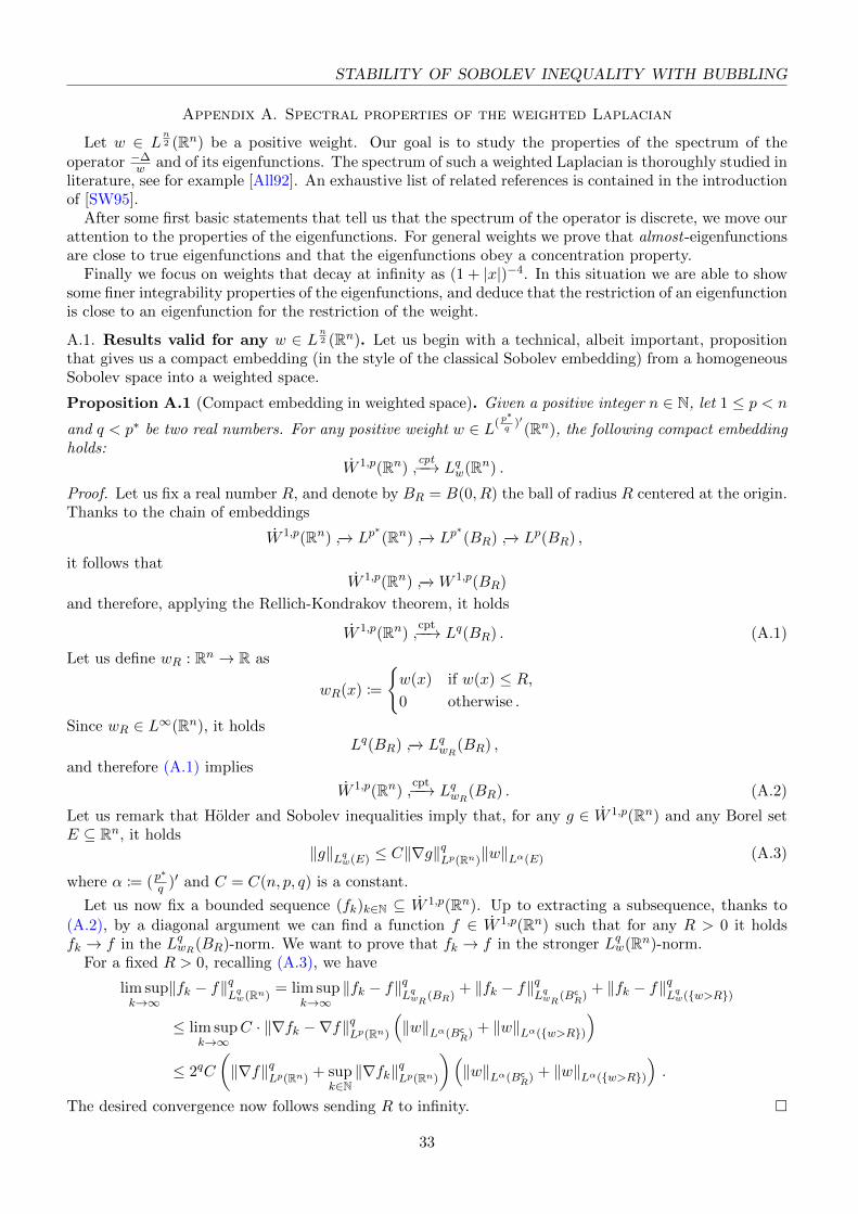
Definition 2.1 (Homogeneous Sobolev space). For any 1 ≤ p < ∞, the homogeneous Sobolev space

W 1,p(Rn) is the closure of C∞c (Rn) with respect to the norm

‖u‖W 1,p := ‖∇u‖Lp .

The space W 1,2(Rn) will be called H1(Rn).

Usually the notation H1(Rn) is adopted to denote W 1,2, we decided to drop the dot as we will neveruse the standard W 1,2.

Definition 2.2 (Weighted Lebesgue space). Let E ⊆ Rn be a Borel set and let w ∈ L1loc(E) be a positive

function. For any 1 ≤ p < ∞, the weighted Lebesgue space Lpw(E) is the space of measurable functionsf : E → R such that ˆ

E|f |pw <∞ .

The norm on Lpw(E) is

f 7→ ‖f‖Lpw(E) =

(Êfpw

) 1p

.

The reason why weighted spaces happen to play a role in our treatment will be evident in Section 2.2.

6


2.1. Symmetries of the problem. Given λ > 0 and z ∈ Rn, let Tz,λ : C∞c (Rn) → C∞c (Rn) be theoperator defined as

Tz,λ(ϕ)(x) := λn−22 ϕ(λ(x− z)) .

The operator Tz,λ satisfies a multitude of properties.

• For any couple of functions ϕ,ψ ∈ C∞c (Rn), it holds

Tz,λ(ϕ · ψ)(x) = Tz,λ(ϕ)(x) · ψ(λ(x− z)) .

• Given k ∈ N, for any choice of positive exponents (ei)1≤i≤k with e1 + · · · + ek = 2∗, and for anychoice of nonnegative functions ϕ1, . . . , ϕk ∈ C∞c (Rn), it holdsˆ

RnTz,λ(ϕ1)e1 · · ·Tz,λ(ϕk)

ek =

ˆRnϕe11 · · ·ϕ

ekk

and in particular ˆRnTz,λ(ϕ)2∗ =

ˆRnϕ2∗

for any ϕ ∈ C∞c (Rn).• For any pair of functions ϕ,ψ ∈ C∞c (Rn) it holdsˆ

Rn∇Tz,λ(ϕ) · ∇Tz,λ(ψ) =

ˆRn∇ϕ · ∇ψ

and in particular ˆRn|∇Tz,λ(ϕ)|2 =

ˆRn|∇ϕ|2 .

• As a consequence of their definition, the Talenti bubbles satisfy

U [z, λ] = Tz,λ(U [0, 1]) and ∂λU [z, λ] =1

λTz,λ(∂λU [0, 1]) .

Obviously all the mentioned properties hold also if the functions are not smooth with compact support,provided that the involved integrals are finite.

The transformations Tz,λ play a central role in the study of the Sobolev inequality as they do notchange the two quantities ‖ϕ‖L2∗ and ‖∇ϕ‖L2 . In particular we will often use this symmetries to reduceourselves to the situation where, instead of considering a generic Talenti bubble, we can take the bubbleU [0, 1].

2.2. Properties and spectrum of(−∆w

)−1. Both in Section 3 and in the construction of the counterex-

ample (Section 4), a fundamental role will be played by the spectrum of( −∆Up−1

)−1where U is a Talenti

bubble, and more in general by the spectrum of the operator(−∆w

)−1where w ∈ L

n2 (Rn) is a suitable

positive weight.

We note that operator(−∆w

)−1is well-defined, compact, and self-adjoint from L2

w(Rn) into L2w(Rn),

therefore it has a discrete spectrum. This fundamental fact, together with many more properties of thespectrum, is contained in Appendix A. We will always consider the the eigenvalues of −∆

w instead of thoseof the inverse operator. We adopt this convention as it is more natural to write −∆ψ = λwψ comparedto −λ∆ψ = wψ.

The properties of the spectrum of( −∆Up−1

)−1, where U is a Talenti bubble, have already been investigated

in [BE91, Appendix].

3. Sharp stability in dimension 3 ≤ n ≤ 5

In this whole section we consider the dimension n and the number of bubbles ν as fixed. Thereforeconstants that depend only on n and ν can be hidden in the notation . and ≈. More precisely, we writethat a . b (resp. a & b) if a ≤ Cb (resp. Ca ≥ b) where C is a constant depending only on the dimensionn and on the number of bubbles ν. Also, we say that a ≈ b if a . b and a & b.

We will deal with weakly-interacting family of Talenti bubbles. A family {U [zi, λi]}1≤i≤ν is weakly-interacting if either the centers zi of the Talenti bubbles are very far one from the other, or their scaling

7


factors λi have different magnitude. It is useful to give a quantitative definition of the amount of interactionthat a certain family of Talenti bubbles has.

Definition 3.1 (Interaction of Talenti bubbles). Let U1 = U [z1, λ1], . . . , Uν = U [zν , λν ] be a family ofTalenti bubbles. We say that the family is δ-interacting for some δ > 0 if

min

(λiλj,λjλi,

1

λiλj |zi − zj |2

)≤ δ . (3.1)

If together with the family we have also some positive coefficients α1, . . . , αν ∈ R, we say that the familytogether with the coefficients is δ-interacting if (3.1) holds and moreover

max1≤i≤ν

|αi − 1| ≤ δ .

Remark 3.2. Our definition of δ-interaction between bubbles is tightly linked to the H1-interaction. In-deed, if U1 = U [z1, λ1], U2 = U [z2, λ2] are two bubbles, thanks to Proposition B.2 it holds (recall that−∆U1 = Up1 )

ˆRn∇U1 · ∇U2 =

ˆRnUp1U2 ≈ min

(λ1

λ2,λ2

λ1,

1

λ1λ2|z1 − z2|2

)n−22

.

In particular, if U1 and U2 belong to a δ-interacting family then their H1-scalar product is bounded by

δn−22 .

3.1. Main Theorem. We are ready to state and prove our main theorem in low dimension (3 ≤ n ≤ 5).We want to show that, in a neighborhood of a weakly-interacting family of Talenti bubbles, the quantity‖∆u+ u|u|p−1‖H1 controls the H1-distance of u from the manifold of sums of Talenti bubbles.

Let us briefly describe the structure of the proof. First we consider the sum of Talenti bubbles σ thatminimizes the distance from u. Then, setting u = σ + ρ, we test ∆u + u|u|p−1 against ρ. Doing so weobtain an estimate on ‖∇ρ‖L2 (namely (3.9)). From there, we estimate the right-hand side of (3.9) with(3.15) to reduce the statement to the validity of the two nontrivial inequalities (3.16) and (3.17). Theproofs of the two mentioned inequalities are postponed to the subsequent sections.

We note that first part of the strategy follows the approach used in [CFM17] to deal with the simplercase of a single bubble (ν = 1).

Theorem 3.3. For any dimension 3 ≤ n ≤ 5 and ν ∈ N, there exist a small constant δ = δ(n, ν) > 0 anda large constant C = C(n, ν) > 0 such that the following statement holds. Let u ∈ H1(Rn) be a functionsuch that ∥∥∥∥∥∇u−

ν∑i=1

∇Ui

∥∥∥∥∥L2

≤ δ ,

where (Ui)1≤i≤ν is a δ-interacting family of Talenti bubbles. Then there exist ν Talenti bubbles U1, U2, . . . , Uνsuch that ∥∥∥∥∥∇u−

ν∑i=1

∇Ui

∥∥∥∥∥L2

≤ C‖∆u+ u|u|p−1‖H−1 .

Furthermore, for any i 6= j, the interaction between the bubbles can be estimated asˆRnUpi Uj ≤ C‖∆u+ u|u|p−1‖H−1 . (3.2)

Proof. In our approach, first we approximate u not only with sums of Talenti bubbles, but even with linearcombinations of them. A posteriori we show that we can recover the result for sums. Adding the degree offreedom of choosing the coefficients of the linear combination gives us the fundamental information (3.6),but at the same time it compels us to prove that in the optimal choice the coefficients are (approximately)1 (see Proposition 3.11).

8


Let σ =∑ν

i=1 αiU [zi, λi] be the linear combination of Talenti bubbles that is closest to u in the H1-norm, that is

‖∇u−∇σ‖L2 = minα1,...,αν∈R

z1,...,...,zν∈Rnλ1,...,λν

∥∥∥∥∥∇u−∇(

ν∑i=1

αiU [zi, λi]

)∥∥∥∥∥L2

.

Let ρ := u− σ be the difference between the original function and the best approximation. Moreover, letus denote Ui := U [zi, λi].

From the fact that the H1-distance of u from∑ν

i=1 Ui is less than δ, it follows directly that ‖∇ρ‖L2 ≤ δ.Furthermore, since the bubbles Ui are δ-interacting, the family (αi, Ui)1≤i≤ν is δ′-interacting for some δ′

that goes to zero as δ goes to 0.Summing up, we can say qualitatively that σ is a sum of weakly-interacting Talenti bubbles and that

‖∇ρ‖L2 is small.Since σ minimizes the H1-distance from u, ρ is H1-orthogonal to the manifold composed of linear

combinations of ν Talenti bubbles. Hence, for any 1 ≤ i ≤ ν, the following n+ 2 orthogonality conditionshold: ˆ

Rn∇ρ · ∇Ui = 0 , (3.3)

ˆRn∇ρ · ∇∂λUi = 0 , (3.4)

ˆRn∇ρ · ∇∂zjUi = 0 for any 1 ≤ j ≤ n. (3.5)

Since the functions Ui, ∂λUi, ∂zjUi are eigenfunctions for −∆

Up−1i

, the mentioned orthogonality conditions are

equivalent to ˆRnρUpi = 0 , (3.6)

ˆRnρ ∂λUi U

p−1i = 0 , (3.7)

ˆRnρ ∂zjUi U

p−1i = 0 for any 1 ≤ j ≤ n. (3.8)

Our goal is to show that ‖∇ρ‖L2 is controlled by ‖∆u+ u|u|p−1‖H−1 . To achieve this, let us start by

testing ∆u+ u|u|p−1 against ρ: exploiting the orthogonality condition (3.3) yieldsˆRn|∇ρ|2 =

ˆRn∇u · ∇ρ =

ˆRnu|u|p−1ρ−

ˆρ(∆u+ u|u|p−1)

≤ˆRnu|u|p−1ρ+ ‖∇ρ‖L2‖∆u+ u|u|p−1‖H−1 .

(3.9)

To control the first term, we use the elementary estimates∣∣∣(a+ b)|a+ b|p−1 − a|a|p−1∣∣∣ ≤ p|a|p−1|b|+ Cn

(|a|p−2|b|2 + |b|p

), (3.10)∣∣∣∣∣∣

(ν∑i=1

ai

)∣∣∣∣∣ν∑i=1

ai

∣∣∣∣∣p−1

−ν∑i=1

ai|ai|p−1

∣∣∣∣∣∣ .∑

1≤i 6=j≤ν|ai|p−1|aj | , (3.11)

that hold for any a, b ∈ R and for any a1, . . . , aν ∈ R. Applying (3.10) with a = σ and b = ρ, and (3.11)with ai = αiUi, we deduce∣∣∣∣∣u|u|p−1 −

ν∑i=1

αi|αi|p−1Upi

∣∣∣∣∣ ≤ pσp−1|ρ|+ Cn,ν

(σp−2|ρ|2 + |ρ|p +

∑1≤i 6=j≤ν

Up−1i Uj

)

9


and therefore, recalling (3.6), we find

ˆRnu|u|p−1ρ ≤ p

ˆRnσp−1ρ2 + Cn,ν

(ˆRnσp−2|ρ|3 +

ˆRn|ρ|2

∗+

∑1≤i 6=j≤ν

ˆRn|ρ|Up−1

i Uj

). (3.12)

Some of the terms in the right-hand side can be controlled easily. Applying Holder and Sobolev inequalitieswe get ˆ

Rnσp−2|ρ|3 ≤ ‖σ‖p−2

L2∗ ‖ρ‖3L2∗ . ‖∇ρ‖3L2 ,

ˆRn|ρ|2

∗. ‖∇ρ‖2

∗

L2 ,

ˆRn|ρ|Up−1

i Uj ≤ ‖ρ‖L2∗‖Up−1i Uj‖L(2∗)′ . ‖∇ρ‖L2‖Up−1

i Uj‖L(2∗)′ .

Substituting these estimates into (3.12) gives us



(‖∇ρ‖3L2 + ‖∇ρ‖2

∗

L2 +∑

1≤i 6=j≤ν‖∇ρ‖L2‖Up−1

i Uj‖L(2∗)′

). (3.13)

In order to proceed further let us notice that, thanks to Proposition B.2, for any i 6= j it holds1

‖Up−1i Uj‖L(2∗)′ =

(ˆRnU

(p−1)(2∗)′

i U(2∗)′

j

) 1(2∗)′

≈(ˆ

RnUpi Uj

) (2∗)′(2∗)′

=

ˆRnUpi Uj . (3.14)

Hence (3.13) becomes



(‖∇ρ‖3L2 + ‖∇ρ‖2

∗

L2 +∑

1≤i 6=j≤ν‖∇ρ‖L2

ˆRnUpi Uj

). (3.15)

It remains to estimate´Rn σ

p−1ρ2 and´Rn U

pi Uj . While the control on the first one is by now rather

standard, some new ideas are needed to control the second term. We state here the two inequalities thatwe need to conclude, and we postpone their proofs to Sections 3.3, 3.4, 3.5 and 3.6:

• Provided δ′ is sufficiently small, it holdsˆRnσp−1ρ2 ≤ c(n, ν)

p

ˆRn|∇ρ|2 (3.16)

for some constant c(n, ν) < 1.• Given ε > 0, if δ′ is sufficiently small thenˆ

RnUpi Uj . ε‖∇ρ‖L2 + ‖∆u+ u|u|p−1‖H−1 + ‖∇ρ‖2L2 (3.17)

for any i 6= j.

With these inequalities at our disposal, we can easily conclude the proof. Indeed, choose ε > 0 such thatν2εCn,νC + c(n, ν) < 1, where Cn,ν is the constant that appears in (3.15) and C is the constant hidden in

1This is the only point of the whole proof where the condition on the dimension plays a crucial role. Indeed, when n ≥ 7only the weaker estimate

‖Up−1i Uj‖L(2∗)′ ≈

(ˆRn

Upi Uj

)p−1

�ˆRn

Upi Uj

holds, while for n = 6 we have

‖Up−1i Uj‖L(2∗)′ ≈

(ˆRn

Upi Uj

) ∣∣∣∣log

(ˆRn

Upi Uj

)∣∣∣∣2/3 � ˆRn

Upi Uj ,

and none of these estimates suffices to conclude the proof.

10


the .-notation in the inequality (3.17). Combining (3.16) and (3.17) into (3.15) yieldsˆRnu|u|p−1ρ ≤

(c(n, ν) + ν2εCn,νC

)‖∇ρ‖2L2

+ C ′n,ν

(‖∇ρ‖3L2 + ‖∇ρ‖2

∗

L2 + ‖∇ρ‖L2‖∆u+ u|u|p−1‖H−1

).

Hence, recalling (3.9), we deduce(1− c(n, ν)− ν2εCn,νC

)‖∇ρ‖2L2 . ‖∇ρ‖L2‖∆u+ u|u|p−1‖H−1 + ‖∇ρ‖3L2 + ‖∇ρ‖2

∗

L2 .

Since we can assume that ‖∇ρ‖L2 � 1, it is easy to see that this last inequality implies the desiredestimate

‖∇ρ‖L2 . ‖∆u+ u|u|p−1‖H−1 . (3.18)

Hence, apart from proving the two inequalities (3.16) and (3.17) (that for now we have taken for granted),in order to finish the proof we have to check:

• that the value of all the αi can be replaced with 1;• that (3.2) holds.

Note that, thanks to (3.18), both facts are direct byproducts either of (3.17) or of the full statement ofthe proposition that proves (3.17) (that is Proposition 3.11). Indeed, by the latter proposition and (3.18)

we know |αi − 1| . ‖∆u+ u|u|p−1‖H−1 , so it suffices to consider σ′ =∑ν

i=1 Ui to get that σ′ satisfies allthe desired conditions. �

3.2. Consequences of the main theorem. As a direct consequence of Theorem 3.3 (and of well-knownresults in literature) we can show the following corollary:

Corollary 3.4. For any dimension 3 ≤ n ≤ 5 and ν ∈ N, there exists a constant C = C(n, ν) such thatthe following statement holds. For any nonnegative function u ∈ H1(Rn) such that(

ν − 1

2

)Sn ≤

ˆRn|∇u|2 ≤

(ν +

1

2

)Sn ,

there exist ν Talenti bubbles U1, U2, . . . , Uν such that∥∥∥∥∥∇u−ν∑i=1

∇Ui

∥∥∥∥∥L2

≤ C‖∆u+ up‖H−1 .

Furthermore, for any i 6= j, the interaction between the bubbles can be estimated asˆRnUpi Uj ≤ C‖∆u+ up‖H−1 .

Proof. Our strategy is to apply Theorem 3.3.Up to enlarging the constant C in the statement, we can assume that ‖∆u+ u|u|p−1‖H−1 is smaller

than a fixed ε > 0. Applying [Str08, Chapter III, Theorem 3.1 and Remarks 3.2] (or directly the originalpapers [Str84; GNN79; BC88; Oba62]), we know that for any δ > 0 we can find an ε > 0 such that if

‖∆u+ u|u|p−1‖H−1 ≤ ε then ∥∥∥∥∥∇u−ν∑i=1

∇Ui

∥∥∥∥∥L2

≤ δ ,

where (Ui)1≤i≤ν is a δ-interacting family. This is exactly the hypothesis necessary to apply Theorem 3.3and conclude. �

Remark 3.5. Let us emphasize that Corollary 3.4 would become false if we drop the assumption ofnonnegativity of the function u. Indeed, as shown in [Din86], there exist sign-changing solutions of

−∆u+ u|u|p−1 = 0 with finite energy on Rn that are not Talenti bubbles.

Remark 3.6. Our proof works in any dimension if ν = 1. Indeed, there are only two points in the proofwhere the assumption n ≤ 5 is used:

11


(1) For n > 6 the exponent p is less than 2, and therefore the inequalityˆRnσp−2|ρ|3 ≤ ‖σ‖p−2

L2∗ ‖ρ‖3L2∗

is false. However, one can note that for p < 2 the inequality (3.10) holds also without the term

|a|p−2|b|2, so for n > 6 the term´Rn σ

p−2|ρ|3 is not present.(2) As observed in the footnote before (3.14), the assumption n ≤ 5 is crucial for estimating the

interaction integrals between bubbles. However, if ν = 1 then there are no interaction integralsand thus everything works also in higher dimension.

Thence, we can prove the result for nonnegative functions in arbitrary dimension when only one bubbleis allowed. The following statement, with some minor differences, is the main result of [CFM17]. We stateit here in this slightly different form since it will be convenient later in Section 5.

Corollary 3.7. For any dimension n ≥ 3, there exists a constant C = C(n) such that the followingstatement holds. For any nonnegative function u ∈ H1(Rn) such that

1

2Sn ≤

ˆRn|∇u|2 ≤ 3

2Sn ,

there exists a Talenti bubble U such that

‖∇u−∇U‖L2 ≤ C‖∆u+ up‖H−1 .

Proof. The proof of the statement is identical to the proof of Corollary 3.4, with the only difference that(thanks to Remark 3.6) we can apply Theorem 3.3 for any dimension n ≥ 3 since only one bubble ispresent. �

3.3. The two missing estimates. It remains to prove (3.16) and (3.17). Before proving them, let usshed some light on the reasons why these two inequalities should hold.

The first of the two inequalities is a strengthened Poincare whose validity follows from the spectralproperties of ρ. Indeed, in the simple setting with a single bubble σ = U [0, 1], (3.16) is equivalent toˆ

RnU [0, 1]p−1ρ2 ≤ c

p

ˆRn|∇ρ|2 .

This latter inequality follows from the orthogonality conditions (3.6), (3.7) and (3.8) since U, ∂λU, ∂ziU arethe eigenfunctions of −∆

Up−1 with eigenvalue greater or equal to 1p . For a justification of the last statement,

see for instance [BE91, Appendix]. To handle the fact that in our setting σ can be a linear combinationof multiple bubbles, we make use of a localization argument via partitions of unity that allows us to treateach bubble independently. Although this argument is rather standard and (3.16) is already known (seefor instance [Bah89, Proposition 3.1]), we prefer to write the proof both for the convenience of the readerand also because some of the localization arguments will be useful later.

The estimate (3.17) is of course empty (and thus trivial) if there is a single bubble, hence also thedifficulty of this estimate depends heavily on the presence of multiple bubbles. Exploiting the localizationargument used to prove (3.16), we manage to prove (3.17) by testing −∆u + u|u|p−1 against suitablylocalized versions of U and ∂λU .

Showing (3.17) is the less intuitive and most involved part of the whole proof.

3.4. Localization of a family of bubbles. Given a family of Talenti bubbles σ =∑ν

i=1 αiUi, we wantto build some bump functions Φ1, . . . ,Φν in such a way that, in some appropriate sense, σΦi

∼= αiUi. Theexistence of these bump functions is tightly linked to the fact that the family is δ-interacting for a smallδ. Indeed if, for example, σ = U1 + U2 and U1 = U2 it is clearly impossible to find any region where, inany meaningful sense, σ ∼= U1.

A similar localization argument is present in [Bah89, Proposition 3.1 and Lemma 3.2], where theauthor proves Proposition 3.10. However, as mentioned before, since in any case we need some furtherproperties of the localization in order to prove Proposition 3.11, we decided to include full proofs both ofthe localization argument and of Proposition 3.10.

12


Lemma 3.8. Let n ≥ 1. Given a point x ∈ Rn and two radii 0 < r < R, there exists a Lipschitz bumpfunction ϕ = ϕx,r,R : Rn → [0, 1] such that ϕ ≡ 1 in B(x, r), ϕ ≡ 0 in B(x, R)c, and

ˆRn|∇ϕ|n . log

(R

r

)1−n.

Proof. Without loss of generality we can assume x = 0. We define ϕ as

ϕ(x) :=

1 if |x| ≤ r,log(R)−log(|x|)log(R)−log(r) if r < |x| < R,

0 if R < |x|.

By definition ϕ ≡ 1 in B(0, r) and ϕ ≡ 0 in B(0, R)c. The norm of the gradient of ϕ is 0 outsideB(0, R) \B(0, r), whereas inside that annulus it satisfies

|∇ϕ|(x) = log

(R

r

)−1 1

|x|.

Thus, it holds ˆRn|∇ϕ|n = log

(R

r

)−n ˆB(0,R)\B(0,r)

1

|x|ndx ≈ log

(R

r

)1−n

as desired. �

Lemma 3.9. For any n ≥ 3, ν ∈ N, and ε > 0, there exists δ = δ(n, ν, ε) > 0 such that if U1 =U [z1, λ1], . . . , Uν = U [zν , λν ] is a δ-interacting family of ν Talenti bubbles, then for any 1 ≤ i ≤ ν thereexists a Lipschitz bump function Φi : Rn → [0, 1] such that the following hold:

(1) Almost all mass of U2∗i is in the region {Φi = 1}, that isˆ

{Φi=1}U2∗i ≥ (1− ε)Sn .

(2) In the region {Φi > 0} it holds εUi > Uj for any j 6= i.(3) The Ln-norm of the gradient is small, that is

‖∇Φi‖Ln ≤ ε .

(4) For any j 6= i such that λj ≤ λi, it holds

sup{Φi>0} Uj

inf{Φi>0} Uj≤ 1 + ε .

Proof. Without loss of generality we can show the statement only for one of the indices, say i = ν, andwe can also assume that Uν = U [0, 1]. This second assumption is justified by the observations containedin Section 2.1, since the Ln-norm of the gradient of a function is invariant under scaling. For notationalsimplicity we denote U := Uν .

We fix a small number ε > 0 (that will be fixed at the end of the proof, depending on the parameter εappearing in the statement) and a large parameter R > 1 (R will be fixed later, depending on ε).

If δ is sufficiently small (depending on ε and R), it follows that εU > Uj in B(0, R) for any 1 ≤ j < νsuch that λj < 1 or |zj | > 2R. In other words we are saying that, if the bubbles are sufficiently weakly-interacting, in an arbitrarily large ball U is much larger than every other bubble which is either lessconcentrated or sufficiently far. Moreover, if δ is sufficiently small, since Uj(x) ∼ (λ−1

j + |x− zj |)2−n italso holds

supB(0,R) Uj

infB(0,R) Uj≤ 1 + ε

for any 1 ≤ j < ν such that λj ≤ 1. Hence, it remains to control the bubbles that are not far and thatare more concentrated than U .

13


Let I ⊂ {1, . . . , ν − 1} be the set of indices j such that λj > 1 and |zj | < 2R. For any j ∈ I, letRj ∈ (0, ∞) be the only positive real number such that

ε

(1

1 +R2

)n−22

=

(λj

1 + λ2j |Rj |

2

)n−22

.

Note that if δ is sufficiently small then Rj ≤ ε2 for any j ∈ I. Thus, as a consequence of the definition ofRj , for any j ∈ I it holds εU ≥ Uj in B(0, R) \B(zj , Rj).

We are now in position to define the function Φ = Φν . With the notation ϕx,r,R introduced inLemma 3.8, we define Φ as

Φ := ϕ0,εR,R

∏j∈I

(1− ϕzj ,Rj ,ε−1Rj ) .

Let us check that if R is chosen sufficiently large, then all requirements are satisfied.Since Rj ≤ ε2, it holdsˆ

{Φ<1}U2∗ ≤

ˆB(0,εR)c

U2∗ +∑j∈I

ˆB(zj ,ε−1Rj)

U2∗ ≤ˆB(0,εR)c

U2∗ +∑j∈I

Cn(ε−1Rj

)n≤ˆB(0,εR)c

U2∗ + Cnνεn .

Hence, if ε is sufficiently small, choosing R = R(ε) large enough we obtainˆ{Φ<1}

U2∗ ≤ εSn

and therefore (1) holds.Noticing that {Φ > 0} is contained inside

B(0, R) \⋃j∈I

B(zj , Rj) ,

since inside such region εU ≥ Uj for any 1 ≤ j < ν (by the observations above), also (2) holds.Similarly, since {Φ > 0} is contained into B(0, R), also property (4) is satisfied.Finally, since ϕx,r1,r2(x) ∈ [0, 1] for any choice of the parameters x, x, r1, r2,

|∇Φ(x)| ≤ |∇ϕ0,εR,R(x)|+∑j∈I|∇ϕ0,Rj ,ε−1Rj (x)| for any x ∈ Rn .

Thus, taking into account Lemma 3.8, we deduce

‖∇Φ(x)‖Ln ≤ ‖∇ϕ0,εR,R(x)‖Ln +∑j∈I‖∇ϕ0,Rj ,ε−1Rj (x)‖

Ln≤ C(n)ν log(ε−1)

1n−1 ,

for some dimensional constant C(n). Hence, given ε > 0, it suffices to choose ε small enough to ensure

that C(n)ν log(ε−1)1n−1 ≤ ε and (3). In this way, since ε � ε, also all the other properties hold with ε

replaced by ε. �

3.5. Spectral Inequality. Using the localization devised in Lemma 3.9, the proof of Proposition 3.10follows a very natural path: we localize, apply the spectral inequality for a single bubble, and then sumall the terms to obtain the full estimate.

Proposition 3.10. Let n ≥ 3 and ν ∈ N. There exists a positive constant δ = δ(n, ν) > 0 such thatif σ =

∑νi=1 αiU [zi, λi] is a linear combination of δ-interacting Talenti bubbles and ρ ∈ H1(Rn) satisfies

(3.6), (3.7) and (3.8) with Ui = U [zi, λi], thenˆRnσp−1ρ2 ≤ c

p

ˆRn|∇ρ|2

where c = c(n, ν) is a constant strictly less than 1.

14


Proof. In this proof we will denote with o(1) any quantity that goes to zero when δ goes to zero. LetΦ1, . . . ,Φν be the localization functions built in Lemma 3.9 for a certain ε that depends on δ. It is clearthat we can choose ε = o(1).

Thanks to Lemma 3.9-(2), it holds

ˆRnσp−1ρ2 ≤ (1 + o(1))

ν∑i=1

ˆRn

Φ2i ρ

2Up−1i +

ˆ{∑

Φi<1}σp−1ρ2 . (3.19)

Then, by Lemma 3.9-(1), using Holder and Sobolev inequalities we find

ˆ{∑

Φi<1}σp−1ρ2 ≤

(ˆ{∑

Φi<1}σ2∗) p−1

2∗

‖ρ‖2L2∗ ≤ o(1)‖∇ρ‖2L2 . (3.20)

We now claim that ˆRn

(ρΦi)2Up−1

i ≤ 1

Λ

ˆRn|∇(ρΦi)|2 + o(1)‖∇ρ‖2L2 , (3.21)

where 1Λ is the largest eigenvalue of −∆

Up−1i

that is strictly smaller than 1p . Let us remark that the value of

Λ does not depend on i.This inequality is crucial and is the only one that exploits the orthogonality conditions we are assuming

on ρ. Its proof relies on the fact that ρΦi almost satisfies the orthogonality conditions, and hence thespectral properties of the operator −∆

Up−1i

will give us (3.21).

Let ψ : Rn → R be, up to scaling, one of the functions Ui, ∂λUi, ∂zjUi, with the scaling chosen so that´Rn ψ

2Up−1i = 1. Hence, thanks to the orthogonality conditions (3.6), (3.7) and (3.8), it holds

〈ρΦi, ψ〉L2

Up−1i

=

∣∣∣∣ˆRn

(ρΦi)ψUp−1i

∣∣∣∣ =

∣∣∣∣ˆRnρψUp−1

i (1− Φi)

∣∣∣∣ ≤ ∣∣∣∣ˆ{Φi<1}

ρψUp−1i

∣∣∣∣≤ ‖ρ‖L2∗

(ˆRnψ2Up−1

i

) 12(ˆ{Φi<1}

U2∗i

) 1n

≤ o(1)‖∇ρ‖L2 .

where in the last inequality we applied Lemma 3.9-(1).This proves that ρΦi is almost orthogonal to ψ. Hence, since the functions Ui, ∂λUi, ∂zjUi form an

orthogonal basis for the space of eigenfunctions of −∆

Up−1i

with eigenvalue greater or equal than 1p (see

[BE91, Appendix]), it holdsˆRn

(ρΦi)2Up−1

i ≤ 1

Λ

ˆRn|∇(ρΦi)|2 + o(1)

ˆRn|∇ρ|2

that is exactly (3.21).We now estimate the right-hand side of (3.21). Note thatˆ

Rn|∇(ρΦi)|2 =

ˆRn|∇ρ|2Φ2

i +

ˆRnρ2|∇Φi|2 + 2

ˆRnρΦi∇ρ · ∇Φi , (3.22)

and that the last two terms above can be bounded as follows: for the first one, using Holder and Sobolevinequalities, we have the estimateˆ

Rnρ2|∇Φi|2 ≤ ‖ρ‖2L2∗‖∇Φi‖2Ln ≤ o(1)‖∇ρ‖2L2

while for the second one, since 12∗ + 1

∞ + 12 + 1

n = 1, we findˆRnρΦi∇ρ · ∇Φi ≤ ‖ρ‖L2∗‖Φi‖L∞‖∇ρ‖L2‖∇Φi‖Ln ≤ o(1)‖∇ρ‖2L2 .

Hence (3.22) becomes ˆRn|∇(ρΦi)|2 ≤

ˆRn|∇ρ|2Φ2

i + o(1)‖∇ρ‖2L2 . (3.23)

15


Note that, as a consequence of Lemma 3.9-(2), we know that the various bump functions Φi have disjointsupports, therefore

ν∑i=1

ˆRn|∇ρ|2Φ2

i ≤ˆRn|∇ρ|2 . (3.24)

Thus, combining (3.19), (3.20), (3.21), (3.23) and (3.24) we achieveˆRnσp−1ρ2 ≤ (1 + o(1))

ν∑i=1

ˆRn

Φ2i ρ

2Up−1i + o(1)‖∇ρ‖2L2

≤(

1

Λ+ o(1)

) ν∑i=1

ˆRn|∇(ρΦi)|2 + o(1)‖∇ρ‖2L2 ≤

(1

Λ+ o(1)

) ˆRn|∇ρ|2

that implies the statement because Λ > p. �

3.6. Interaction integral estimate.

Proposition 3.11. Let n ≥ 3 and ν ∈ N. For any ε > 0 there exists δ = δ(n, ν, ε) > 0 such that thefollowing statement holds. Let u =

∑νi=1 αiUi + ρ, where the family (αi, Ui)1≤i≤ν is δ-interacting, and ρ

satisfies both the orthogonality conditions (3.6), (3.7) and (3.8) and the bound ‖∇ρ‖L2 ≤ 1. Then, for any1 ≤ i ≤ ν, it holds

|αi − 1| . ε‖∇ρ‖L2 + ‖∆u+ u|u|p−1‖H−1 + ‖∇ρ‖min(2,p)L2 , (3.25)

and for any pair of indices i 6= j it holdsˆRnUpi Uj . ε‖∇ρ‖L2 + ‖∆u+ u|u|p−1‖H−1 + ‖∇ρ‖min(2,p)

L2 . (3.26)

Proof. In order to handle the cases n ≤ 6 and n > 6 at the same time, in this proof we will highlight as{E}n≤6 the terms E that appear in our estimates only when n ≤ 6 (that is when p ≥ 2).

We consider δ as a parameter and we denote with o(1) any expression that goes to zero when theparameter δ goes to zero. Similarly o(E) denotes any expression that, when divided by E, is o(1).

Let λ1, . . . , λν > 0 and z1, . . . zν ∈ Rn be the parameters such that Ui = U [zi, λi] for any 1 ≤ i ≤ ν.Without loss of generality we can assume λi to be decreasing (i.e. U1 is the most concentrated bubble).We prove the statement by induction on the index i = 1, . . . , ν (starting from the most concentratedbubble).

Let us fix 1 ≤ i ≤ ν and let us assume to know the result for all smaller values of the index. Fornotational simplicity we denote U = Ui, α = αi, and V =

∑j 6=i αjUj . Let Φ = Φi be the bump function

built in Lemma 3.9 for a fixed ε > 0 that depends on δ (and is o(1) by definition).Without loss of generality we can assume Ui = U = U [0, 1]. Indeed, all the quantities involved (α− 1,´

Rn Upi Uj , ‖∇ρ‖L2 , ‖∆u+ u|u|p−1‖H−1) are invariant under the action of the symmetries described in

Section 2.1.We begin from the identity

(α−αp)Up−pαp−1Up−1V = ∆ρ+ (−∆u− u|u|p−1)−∑

αiUpi +p(αU)p−1ρ

+[(σ + ρ)|σ + ρ|p−1−σp−pσp−1ρ

]+[pσp−1ρ−p(αU)p−1ρ

]+[(αU + V )p−(αU)p−p(αU)p−1V

].

(3.27)

Exploiting Lemma 3.9-(2) we can show that, in the region {Φ > 0}, it holds∑j 6=i

αjUpj = o

(Up−1V

),∣∣∣(σ + ρ)|σ + ρ|p−1 − σp − pσp−1ρ

∣∣∣ . |ρ|p +{Up−2|ρ|2

}n≤6

,∣∣pσp−1ρ− p(αU)p−1ρ∣∣ = o(Up−1|ρ|) ,∣∣(αU + V )p − (αU)p − p(αU)p−1V

∣∣ = o(Up−1V

).

16


Thus, applying these estimates in (3.27), we deduce that inside the region {Φ > 0} one has∣∣∣(α− αp)Up − (pαp−1 + o(1))Up−1V −∆ρ− (−∆u− u|u|p−1)− p(αU)p−1ρ∣∣∣

. |ρ|p +{Up−2|ρ|2

}n≤6

+ o(Up−1|ρ|) .(3.28)

In the remaining part of this proof, all integrals are computed on the whole Rn and therefore, fornotational convenience, we do not write explicitly the domain of integration.

Let ξ be either U or ∂λU . What follows holds for both choices.First of all, thanks to the orthogonality conditions (3.3), (3.4), (3.6) and (3.7), recalling (2.1), we know

that Ûp−1ξρ =

ˆ∇ξ · ∇ρ = 0 . (3.29)

Let us test (3.28) against ξΦ. We get∣∣∣∣ˆ [(α− αp)Up − (pαp−1 + o(1))Up−1V]ξΦ

∣∣∣∣.

∣∣∣∣ˆ ∇ρ · ∇(ξΦ)

∣∣∣∣+

∣∣∣∣ˆ (−∆u− u|u|p−1)ξΦ

∣∣∣∣+

∣∣∣∣ˆ Up−1ξρΦ

∣∣∣∣+

ˆ|ρ|p|ξ|Φ +

{Ûp−2|ξ||ρ|2Φ

}n≤6

+ o

(Ûp−1|ξ||ρ|Φ

).

(3.30)

We now exploit (3.29) to bound all the terms appearing in the right-hand side of (3.30):∣∣∣∣ˆ ∇ρ · ∇(ξΦ)

∣∣∣∣ =

∣∣∣∣ˆ ∇ρ · ∇(ξ(Φ− 1))

∣∣∣∣ ≤ ‖∇ρ‖L2‖∇(ξ(Φ− 1))‖L2 ,∣∣∣∣ˆ (−∆u− u|u|p−1)ξΦ

∣∣∣∣ ≤ ‖∆u+ u|u|p−1‖H−1‖∇(ξΦ)‖L2 ,∣∣∣∣ˆ Up−1ξρΦ

∣∣∣∣ =

∣∣∣∣ˆ Up−1ξρ(Φ− 1)

∣∣∣∣ . ‖∇ρ‖L2

(ˆ{Φ<1}

(Up−1|ξ|

) 2∗p

) p2∗

,

ˆ|ρ|p|ξ|Φ ≤

ˆ|ρ|p|ξ| . ‖∇ρ‖p

L2‖ξ‖L2∗ ,{Ûp−2|ξ||ρ|2Φ ≤

Ûp−2|ξ||ρ|2 . ‖∇ρ‖2L2‖Up−2ξ‖

L2∗p−1

}n≤6

,

Ûp−1|ξ||ρ|Φ ≤

Ûp−1|ξ||ρ| . ‖∇ρ‖L2‖Up−1ξ‖

L2∗p

.

(3.31)

Moreover, since ξ is equal either to U or to ∂λU , we have that |ξ| . U pointwise (see (2.2)). Hence,recalling Lemma 3.9-(1) and Lemma 3.9-(3) we obtain

‖∇(ξ(Φ− 1))‖L2 = o(1) , ‖∇(ξΦ)‖L2 . 1 ,

ˆ{Φ<1}

(Up−1|ξ|

) 2∗p = o(1) ,

‖ξ‖L2∗ . 1 , ‖Up−2ξ‖L

2∗p−1. 1 , ‖Up−1ξ‖

L2∗p. 1 .

(3.32)

Using the set of inequalities (3.31) and (3.32), it follows by (3.30) that∣∣∣∣ˆ [(α− αp)Up − (pαp−1 + o(1))Up−1V]ξΦ

∣∣∣∣. o(1)‖∇ρ‖L2 + ‖∆u+ u|u|p−1‖H−1 + ‖∇ρ‖min(2,p)

L2 .

(3.33)

Let us now split V = V1 + V2 where V1 :=∑

j<i αjUj and V2 :=∑

j>i αjUj . Since by induction we can

assume that the statement of the proposition holds for all j < i, and recalling thatÚpi Uj =

´∇Ui ·∇Uj =´

Upj Ui and |ξ| . U , we seeÛp−1V1|ξ|Φ .

ÛpV1 . o(1)‖∇ρ‖L2 + ‖∆u+ u|u|p−1‖H−1 + ‖∇ρ‖min(2,p)

L2 . (3.34)

17


On the other hand, thanks to Lemma 3.9-(4), we know that

V2(x)Φ(x) = (1 + o(1))V2(0)Φ(x) (3.35)

for any x ∈ Rn.We now prove (3.25). If α = 1 there is nothing to prove, so we can assume that α 6= 1 and we define

θ := pαp−1V2(0)α−αp . Recalling (3.34) and (3.35), it follows by (3.33) that

|α− αp|∣∣∣∣ˆ (Up − (1 + o(1))θUp−1)ξΦ

∣∣∣∣ . o(1)‖∇ρ‖L2 + ‖∆u+ u|u|p−1‖H−1 + ‖∇ρ‖min(2,p)L2 . (3.36)

This latter inequality is very strong since it holds both with ξ = U and ξ = ∂λU , with the constant θindependent of this choice. Since Φ is identically 1 on a large ball centered at 0 where U has almost allthe mass (see Lemma 3.9-(1)), we haveˆ (

Up − (1 + o(1))θUp−1)ξΦ =

Ûpξ − θ

Ûp−1ξ + o(1) . (3.37)

Our goal is to show that the right-hand side cannot be very small both when ξ = U and when ξ = ∂λU .In order to achieve this, it suffices to check that´

U2∗Úp6=Úp∂λUÚp−1∂λU

. (3.38)

Note that the left-hand side is clearly positive, while the right-hand side is equal to zero. IndeedÚp∂λU

is the derivative with respect to λ of 12∗

Ú [0, λ]2

∗which is independent of λ (see Section 2.1), hence´

Up∂λU = 0, while

p

Ûp−1∂λU =

d

dλ

∣∣∣λ=1

Û [0, λ]p =

d

dλ

∣∣∣λ=1

(λ

2−n2

Û [0, 1]p

)=

2− n2

Ûp 6= 0 .

Thus, as a consequence of (3.37) and (3.38) we deduce that

maxξ∈{U,∂λU}

(∣∣∣∣ˆ (Up − (1 + o(1))θUp−1)ξΦ

∣∣∣∣) & 1

and therefore, choosing ξ so that the maximum above is attained, (3.36) implies (3.25).Now that we have proven (3.25), choosing ξ = U in (3.33) we obtain∣∣∣∣ˆ UpV Φ

∣∣∣∣ . o(1)‖∇ρ‖L2 + ‖∆u+ u|u|p−1‖H−1 + ‖∇ρ‖min(2,p)L2

and in particular ∣∣∣∣∣ˆB(0,1)

UpUj

∣∣∣∣∣ . o(1)‖∇ρ‖L2 + ‖∆u+ u|u|p−1‖H−1 + ‖∇ρ‖min(2,p)L2

for any j 6= i. Thanks to Corollary B.4, we deduce (3.26) for all j > i. Since for j < i we already knowthe validity of (3.26) by the induction (recall that

ÚpUj =

Úpj U), this concludes the proof. �

4. Counterexample in dimension n ≥ 6

In this section we show that Theorem 3.3 does not hold when the dimension n is strictly above 5. Theexact statement we want to prove is the following.

Theorem 4.1. For any dimension n ≥ 6, there exists a family of functions uR ∈ H1(Rn) parametrizedby a positive real number R > 1 such that the following statement holds.

For any choice of the parameters α, β, λ1, λ2 > 0 and z1, z2 ∈ Rn, if we denote σ′ := αU [z1, λ1] +βU [z2, λ2], then

‖∆uR + uR|uR|p−1‖L(2∗)′ . ζn(∥∥∇uR −∇σ′∥∥L2) ,

18


where ζn : (0, ∞)→ (0, ∞) is defined as

ζn(t) :=

t

|log(t)| if n = 6,

t109 if n = 7,

t65 |log(t)| if n = 8,

tn+4n+2 if n > 8.

Furthermore, when we let R→∞, the family uR satisfies

‖∇uR −∇U [−Re1, 1]−∇U [Re1, 1]‖L2 → 0 ,

where e1 = (1, 0, . . . , 0) is the first vector of the canonical basis of Rn.In particular, Theorem 3.3 cannot hold when n ≥ 6.

Remark 4.2. As can be seen from the statement, we prove more than the failure of Theorem 3.3. Indeedthe counterexample is stronger than needed for the following reasons:

• The H−1-norm is replaced with the stronger L(2∗)′-norm.• When n ≥ 7, we show the existence of an exponent γ > 1 such that Theorem 3.3 remains false

even if ‖∆u+ u|u|p−1‖H−1 is raised to the power 1γ′ with γ′ < γ. This shows that the infimum of

the exponents that make Theorem 3.3 true, if it exists, is greater than 1 when n ≥ 7.• We allow the freedom to choose the coefficients in front of the Talenti bubbles.

Moreover, the counterexample is “as simple as it can be”. In fact, in the neighborhood of a single bubbleTheorem 3.3 holds in every dimension, as observed in the paragraph before Corollary 3.7. Therefore atleast two bubbles are required for a counterexample, and indeed our construction uses exactly two bubbles(that is ν = 2 in the statement of Theorem 3.3).

Nonetheless, Theorem 4.1 is not entirely satisfying. In fact, as mentioned in the introduction, Struwe’sTheorem 1.1 (and then Corollary 3.4) deals with nonnegative functions. This shortcoming is solved bythe following theorem that shows the existence of a nonnegative counterexample, which negates also thevalidity of Corollary 3.4 when the dimension is strictly larger than 5.

Theorem 4.3. For any dimension n ≥ 6, there exists a family of nonnegative functions u+R ∈ H1(Rn)

parametrized by a positive real number R > 1 such that the following statement holds.For any choice of the parameters α, β, λ1, λ2 > 0 and z1, z2 ∈ Rn, if we denote σ′ := αU [z1, λ1] +

βU [z2, λ2], it holds‖∆u+

R + (u+R)p‖H−1 . ξn(

∥∥∇u+R −∇σ

′∥∥L2) ,

where ξn(t) :=√tζn(t), and ζn is the function defined in Theorem 4.1. Furthermore, when we let R→∞,

the family satisfies‖∇u+

R −∇U [−Re1, 1]−∇U [Re1, 1]‖L2 → 0 , (4.1)

where e1 = (1, 0, . . . , 0) is the first vector of the canonical basis of Rn.In particular, Corollary 3.4 cannot hold when n ≥ 6.

Remark 4.4. Note that in Theorem 4.3 we use again the H−1-norm (instead of the L(2∗)′-norm used inTheorem 3.3). Moreover the dependence given by ξn is slightly worse than the dependence given by ζn(that, most likely, was already non-optimal).

The notation u+R is significative not only of the nonnegativity of the counterexample, but also of the

way it is constructed: it is exactly the positive part of the counterexample uR built in Theorem 4.1.Let us remark that, perturbing suitably a family of nonnegative functions that satisfies Theorem 4.3,

we can easily obtain a family of positive functions that still satisfies Theorem 4.3. Hence Theorem 4.3holds even if the functions are required to be strictly positive.

Let us sketch briefly how the counterexample is built. From now on we will not show explicitly thedependence of our construction from the real parameter R > 0 (so we will write u in place of uR).Moreover, unless stated otherwise, the dimension n will always be greater or equal than 6.

Let us fix two Talenti bubbles U = U [−Re1, 1] and V = [Re1, 1]. The idea is to linearize the equation

∆u+u|u|p−1 = 0 when u is close to U +V . Hence, let u = U +V +ρ. We shall ask ρ to be H1-orthogonalto the manifold of linear combinations of two Talenti bubbles (see (3.3), (3.4) and (3.5)). Indeed, under

19


this assumption we shall have that ‖∇ρ‖L2 ≈ d(u), where d(u) is the H1-distance between u and themanifold of all linear combinations of two Talenti bubbles.

Thanks to the estimate (see (4.7) below)

‖∆u+ u|u|p−1‖L(2∗)′ = ‖∆ρ+ ((U + V )p − Up − V p) + p(U + V )p−1ρ‖L(2∗)′ +O(‖∇ρ‖pL2) ,

if we were able to solve ∆ρ + ((U + V )p − Up − V p) + p(U + V )p−1ρ = 0, we would have finished. Un-fortunately this is not possible because there are some nontrivial obstructions (that are a consequence ofthe orthogonality conditions we are imposing on ρ) related to the spectrum of −∆

(U+V )p−1 .

For this reason, we consider instead a perturbation f of f := (U + V )p − Up − V p such that ∆ρ +

f + p(U + V )p−1ρ = 0 becomes solvable. We build f as a suitable projection of f onto a subspace ofeigenfunctions of −∆

(U+V )p−1 . This will allow us to prove the desired controls on ρ, from which we will

deduce that u = U + V + ρ is the sought counterexample.To be precise, we should say that the function ρ that we are going to construct does not satisfy exactly

the orthogonality conditions mentioned above. Nonetheless, we will be able to show (through a series ofdelicate properties of eigenspaces of close-by operators) that it almost satisfies these conditions, and thiswill be enough to show that the distance of u from the manifold of linear combinations of two Talentibubbles cannot be much less than ‖∇ρ‖L2 .

Let us remark that our construction is not explicit, as it depends on the solution of a partial differentialequation.

4.1. Notation and definitions for the counterexample. The dimension n ≥ 6 will be consideredfixed, and all constants are implicitly allowed to depend on the dimension. Let us fix ε = ε(n) such that

(1− ε)2 = pΛ , where Λ−1 is the largest eigenvalue of

(−∆

U [0,1]p−1

)−1below 1

p . Our choice of ε ensures that

p

p(1− ε)−1= 1− ε and

p(1− ε)−1

Λ= 1− ε . (4.2)

Let U = U [−Re1, 1] and V = [Re1, 1] be two Talenti bubbles. Our constructions and definitions dependon a real parameter R � 1. The dependence from R will not be explicit in our notation (that is, wewill not add an index R everywhere). Given two expressions A and B (that depend on R), the notationA = o(B) means that there exists a function ω : (0, ∞)→ (0, ∞) such that ω(R)→ 0 when R→∞ andA ≤ ω(R)B.

Let us now introduce two subspaces of L2(U+V )p−1(Rn).

Let E be the subspace generated by all eigenfunctions of(

−∆(U+V )p−1

)−1with eigenvalue larger than 1−ε

p ,

and fix an orthonormal basis BE of E made of eigenfunctions of(

−∆(U+V )p−1

)−1. Note that, since this basis

is made of eigenfunctions, the functions in BE are orthogonal also with respect to the H1-scalar product.

Let F be the subspace generated by all eigenfunctions of( −∆Up−1

)−1and

( −∆V p−1

)−1with eigenvalue larger

than 1−εp . Let us recall (see [BE91, Appendix]) that the set BF composed of the 2(1 + 1 + n) functions

BF :=

{U, ∂λU, ∂ziU, V, ∂λV, ∂ziV

}is a basis of F . Such a basis is not orthonormal (or orthogonal) with respect to neither the L2

(U+V )p−1-

scalar product nor the H1-scalar product. Nonetheless, if we let R go to infinity, the L2(U+V )p−1-scalar

product between two functions in BF converges to 0 and the L2(U+V )p−1-norms of all those functions

converge to some positive values. The same properties hold also for the H1-norm. We will refer to theseproperties saying that BF is asymptotically quasi-orthonormal with respect to both the L2

(U+V )p−1-scalar

product and the H1-scalar product.

20


Let π : L2(U+V )p−1(Rn) → L2

(U+V )p−1(Rn) be the projection on the subspace orthogonal to E (with

respect to the L2(U+V )p−1-scalar product), set f := (U + V )p − Up − V p, and define

f := (U + V )p−1 · π(

f

(U + V )p−1

).

Remark 4.5. Our choice of f ensures (by construction) that f is orthogonal, in the L2-scalar product, to

E . Since this is fundamentally the only property that we need on f , one could also be tempted to definef as the projection, with respect to the L2-scalar product, onto the subspace L2-orthogonal to E . Thesetwo definitions are not the same and we have chosen ours because it allows us to prove Lemma 4.11 (whileit is not clear to us how to prove Lemma 4.11 with the other definition).

Let us define the function ρ ∈ L2(U+V )p−1(Rn) as the unique solution of

∆ρ+ p(U + V )p−1ρ+ f = 0 (4.3)

such that π(ρ) = ρ (namely ρ is orthogonal, in the L2(U+V )p−1-scalar product, to E). The existence of ρ

can be justified as follows. If we denote T =(

−∆(U+V )p−1

)−1, then (4.3) is equivalent to

(1− pT )ρ = T

(π

(f

(U + V )p−1

)).

Since π is the projection into E⊥ and E is an eigenspace for the self-adjoint operator T , the right-handside belongs to E⊥. Let T |E⊥ denote the restriction of the operator T on the subspace E⊥. Since (bydefinition of E) T |E⊥ has eigenvalues strictly smaller than 1−ε

p , it follows that 1− pT |E⊥ : E⊥ → E⊥ is an

isomorphism. Thus there exists a unique solution ρ ∈ E⊥ given by

ρ := (1− pT |E⊥)−1 T |E⊥(π

(f

(U + V )p−1

)).

With this definition, we set u := U + V + ρ.

4.2. First observations. Before going into the technical details of the proof, let us remark some prop-erties that will be crucial later on.

First of all, thanks to Lemma A.5, since π(ρ) = ρ it holds

‖∇ρ‖L2 ≈ ‖f‖H−1 . (4.4)

Also, recalling (4.3), the identity

∆u+ u|u|p−1 =[f − f

]+[(U + V + ρ)|U + V + ρ|p−1 − (U + V )p − p(U + V )p−1ρ

](4.5)

holds. Moreover, since 1 < p ≤ 2, we have the pointwise elementary estimate∣∣∣(U + V + ρ)|U + V + ρ|p−1 − (U + V )p − p(U + V )p−1ρ∣∣∣ . |ρ|p . (4.6)

In particular, combining (4.5) and (4.6) and applying the Sobolev inequality, we deduce

‖∆u+ u|u|p−1‖L(2∗)′ ≤ ‖f − f‖L(2∗)′ + ‖ρp‖L(2∗)′ . ‖f − f‖L(2∗)′ + ‖∇ρ‖pL2 . (4.7)

Hence, the main challenge is to estimate ‖f − f‖L(2∗)′ . This is done in the next sections, where we provethe crucial estimate in Lemma 4.12.

Finally, as already mentioned before, let us emphasize that our choice of ρ does not satisfy the or-thogonality conditions we would desire (namely ρ is not orthogonal to F with respect to the H1-scalarproduct). Nonetheless, we will show that it is almost orthogonal and this will suffice to deduce that thefunction u provides the desired family of counterexamples. For this the first important step is to estimatethe distance between the subspaces E and F . This is the purpose of the next subsection.

21


4.3. The subspaces E and F are very close. When R > 0 is large, since Up−1 and V p−1 are concen-trated in regions distant one from the other, it is natural to expect that the lowest section of the spectrumof −∆

(U+V )p−1 is approximately the sum of the lowest parts of the spectra of −∆Up−1 and −∆

V p−1 . Thus the two

subspaces E and F should have the same dimension and be, in some appropriate sense, very close one tothe other. This subsection is devoted exactly to this: formalizing and proving the mentioned ansatz.

Let us begin introducing a distance between subspaces of a Hilbert space. This definition is classical,see [Mor10, Equation (3)] and the references therein for the proofs of the properties we are going to state.

Definition 4.6. Let E,F be two finite subspaces of a Hilbert space X. The distance d(E,F ) betweenthem is defined as

d(E,F ) := dH({|x| ≤ 1} ∩ E, {|x| ≤ 1} ∩ F

),

where dH denotes the Hausdorff distance.

This notion of distance enjoys a number of nice properties. We list some of them:

• For any two subspaces E and F it holds d(E,F ) ≤ 1.• If two subspaces E and F have different dimensions, then d(E,F ) = 1.• There are several equivalent definitions of such distance involving orthogonal projections. More

precisely, given two subspaces E and F , let πE : X → E and πF : X → F be the orthogonalprojections onto E and F , respectively. Then the following identity holds:

d(E,F ) = ‖πE − πF ‖op ,

where ‖ · ‖op is the operator norm. Moreover, it also holds

d(E,F ) = max

(sup

e∈E\{0}

|e− πF (e)||e|

, supf∈F\{0}

|f − πE(f)||f |

).

If dimE = dimF , then the two suprema in the last formula are equal and it holds

d(E,F ) = supe∈E\{0}

|e− πF (e)||e|

= supf∈F\{0}

|f − πE(f)||f |

.

• The distance does not change if we replace E,F with E⊥ and F⊥, that is

d(E,F ) = d(E⊥, F⊥) .

We are ready to prove that E and F are close with respect to the distance defined above. The proof isbased on a series of technical tools that are postponed to Appendix A.

Proposition 4.7. For any sufficiently large R we have dim E = dimF = 2n+ 4 and

d(E ,F) = o(1) ,

where the distance on the subspaces is induced by the L2(U+V )p−1-norm.

Proof. Let us notice that the subspace F is the direct sum of the two subspaces FU and FV that are

generated by the eigenfunctions of( −∆Up−1

)−1and

( −∆V p−1

)−1with eigenvalue larger than 1−ε

p . The two

bases BE and BF are respectively orthonormal and asymptotically quasi-orthonormal with respect to theL2

(U+V )p−1-scalar product (see Section 4.1), hence the statement is equivalent to showing the following two

facts:

(1) For any ψ ∈ BE there exists ψ′ ∈ F such that ‖ψ − ψ′‖L2(U+V )p−1

= o(1).

(2) For any ψ ∈ BF there exists ψ′ ∈ E such that ‖ψ − ψ′‖L2(U+V )p−1

= o(1).

We begin by proving (2). Without loss of generality we can assume ψ ∈ BF ∩ FU . Therefore it holds−∆ψ = λUp−1ψ with λ ∈ {1, p}, and rearranging the terms we get

−∆ψ − λ(U + V )p−1ψ = λ(Up−1 − (U + V )p−1

)ψ .

We can now apply Lemma A.4 in conjunction with Corollary A.8 to obtain∑k

α2k

(1− λ

λk

)2

. ‖(Up−1 − (U + V )p−1

)ψ‖

L2 = o(1) ,

22


where ψ =∑αkψk and (λ−1

k , ψk) is the sequence of eigenvalues and normalized eigenfunctions of the

operator(

−∆(U+V )p−1

)−1. Choosing ψ′ := πE(ψ) as the projection of ψ onto E we have

ψ′ =∑

λk<p(1−ε)−1

αkψk ,

and thus

‖ψ − ψ′‖2L2(U+V )p−1

=∑

λk≥p(1−ε)−1

α2k ≤

1

ε2

∑λk≥p(1−ε)−1

α2k

(1− λ

λk

)2

= o(1) ,

that is exactly the statement of (2).The proof of (1) is similar to the one of (2); the main difference being that, instead of Lemma A.4, we will

use Proposition A.10. Let us consider ψ ∈ BE that solves −∆ψ = λ(U +V )p−1ψ with 0 < λ < p(1− ε)−1.Define two functions ϕU and ϕV as

ϕU (x) := ψ(x) η

(x+Re1

R/2

), ϕV (x) := ψ(x) η

(x−Re1

R/2

),

where η is a smooth bump function as described in the statement of Proposition A.10. If we applyProposition A.10 and we follow the same reasoning we have used to prove (2) (recalling (4.2)), we findtwo functions ψU ∈ FU and ψV ∈ FV such that

‖ψU − ϕU‖L2Up−1

= o(1) , ‖ψV − ϕV ‖L2V p−1

= o(1) .

Since ϕU is supported inside the set {U ≥ V } and ϕV is supported inside {V ≥ U}, the previous estimatescan be upgraded to

‖ψU − ϕU‖L2(U+V )p−1

. ‖ψU − ϕU‖L2Up−1

+ ‖ψU‖L2V p−1

= o(1) ,

‖ψV − ϕV ‖L2(U+V )p−1

. ‖ψV − ϕV ‖L2V p−1

+ ‖ψV ‖L2Up−1

= o(1) .(4.8)

Let us define ψ′ := ψU + ψV . Of course it holds ψ′ ∈ F . Then, by the triangle inequality and (4.8), weobtain

‖ψ − ψ′‖L2(U+V )p−1

≤ o(1) + ‖ψ − ϕU − ϕV ‖L2(U+V )p−1

≤ o(1) +

ˆRn\[B(−Re1,R/2)∪B(Re1,R/2)]

ψ2(U + V )p−1 .

The proof is finished since also the last integral is o(1) thanks to Lemma A.6. �

Remark 4.8. The statement of Proposition 4.7 can be generalized to cover much more general situations.Even if we will not need it, let us give a possible generalization.

For a fixed n ≥ 5, let (wk)k∈N ⊆ Ln2 (Rn) be a sequence of positive weights of the form wk =∑ν

i=1 U [x(k)i , λi]

p−1, where (λi)1≤i≤ν are fixed and (x(k)i )1≤i≤ν,k∈N is a sequence of ν-tuples of points

in Rn such that |x(k)i − x

(k)j | → ∞ for any i 6= j. For a fixed µ > 0, let E(k)

µ be the subspace of the

eigenfunctions of(−∆wk

)−1with eigenvalue greater or equal than µ−1, and let F (k)

µ,i be the subspace of

the eigenfunctions of

(−∆

U [x(k)i ,λi]p−1

)−1

with eigenvalue greater or equal than µ−1. Then, if µ−1 is not an

eigenvalue for(

−∆U [0,1]p−1

)−1, it holds

d(E(k)µ ,F (k)

µ,1 ⊕ · · · ⊕ F(k)µ,ν

)→ 0 ,

where the distance between subspaces is induced by the L2wk

-norm.With some care it would be possible to obtain a similar result also for weights much more general than

finite sums of Talenti bubbles (in the spirit of Proposition A.10). We will not do that, as it is out of thescope of this note.

23


4.4. The norm of ρ is asymptotically larger than ||∆u+ u|u|p−1||L(2∗)′ . Our intuition tells us that

‖∇ρ‖L2 gives a good approximation of the H1-distance of u from the manifold of linear combinations oftwo Talenti bubbles. Thus, since our final goal is proving that such a distance is asymptotically largerthan ‖∆u+ u|u|p−1‖L(2∗)′ , we devote this section to the proof that ‖∇ρ‖L2 is asymptotically larger than

‖∆u+ u|u|p−1‖L(2∗)′ .Our approach is very direct: we compute all the involved quantities and, in the end, compare them.Let us emphasize that the elementary and explicit estimate

‖f‖L2 = o(‖f‖H−1) ,

where f = (U +V )p−Up−V p, is fundamentally equivalent to what we want to prove. The validity of thementioned estimate (that follows from Lemmas 4.9 and 4.10 below) depends heavily on the dimensionalcondition n ≥ 6.

Lemma 4.9. It holds

‖f‖H−1 &

{R−4 log(R)

12 if n = 6,

R−n+22 if n ≥ 7.

Proof. First we deal with the easier case n ≥ 7. Let us fix a smooth bump function η ∈ C∞c (Rn) suchthat 0 ≤ η ≤ 1 everywhere, η ≡ 1 in B(1, 1

4), and η ≡ 0 in B(1, 12)c. In B(4Re1, R) the function f is

comparable to R−n−2 (that coincides with the decay of U [0, 1]p), hence it holds

R−2 = Rn ·R−n−2 .ˆRnf(x) η

( x

4R

)dx ≤ ‖f‖H−1

∥∥∥∇(η ( ·4R

))∥∥∥L2. R

n−22 ‖f‖H−1

that gives

R−n+22 . ‖f‖H−1 ,

as desired.When n = 6, we prove the result testing f against the function f

12 . Let us remark that, since n = 6, it

holds 2∗ = 3, p = 2, and thus in particular f = 2UV .We have ˆ

R6

U32V

32 . ‖f‖H−1

(ˆR6

|∇(f12 )|

2) 1

2

. (4.9)

We estimate independently the left-hand side and the right-hand side.Applying Proposition B.2 with parameters α = β = 3

2 yieldsˆR6

U32V

32 ≈ R−6 log(R) . (4.10)

On the other hand it holds

|∇(f12 )|

2≈ |∇U |2U−1V + |∇V |2V −1U

and, since |∇U | ≈ Un−1n−2 = U

54 , we obtain

|∇(f12 )|

2≈ U

32V + UV

32 .

Thus, applying Proposition B.5 with a = c = 32 and b = d = 1, we deduce(ˆ

R6

|∇(f12 )|

2) 1

2

≈(ˆ

R6

U32V

) 12

≈(R−4 log(R)

) 12 ≈ R−2 log(R)

12 . (4.11)

Finally, combining (4.9), (4.10) and (4.11) we get

R−6 log(R) . ‖f‖H−1 ·R−2 log(R)12 ,

that implies the desired estimate. �

24


Lemma 4.10. It holds

‖f‖L2 ≈

R−4 if n = 6,

R−5 if n = 7,

R−6 log(R)12 if n = 8,

R−n+42 if n > 8.

Proof. We note that ‖f‖2L2 =´Rn ϕ(U, V ) where

ϕ(x, y) = ((x+ y)p − xp − yp)2 .

The mentioned function ϕ satisfies the hypotheses of Proposition B.5 with a = 2p − 2, b = 2, c = 2, d =

2p− 2. Hence ‖f‖2L2 ≈ ΦR(2p− 2, 2, 2, 2p− 2), and computing the value of ΦR(2p− 2, 2, 2, 2p− 2)12 yields

the desired result. �

Lemma 4.11. It holds‖f − f‖L(2∗)′ . ‖f‖L2 .

Proof. By definition of f , we have

f − f = (U + V )p−1

(f

(U + V )p−1− π

(f

(U + V )p−1

))= (U + V )p−1

∑ψE∈BE

〈 f

(U + V )p−1, ψE〉L2

(U+V )p−1ψE

= (U + V )p−1∑

ψE∈BE

〈f, ψE〉L2 ψE .

Thus, taking the L(2∗)′-norm and applying Holder’s inequality with exponents 12 + 1

n = 1(2∗)′ , we obtain

‖f − f‖L(2∗)′ ≤∑

ψE∈BE

|〈f, ψE〉L2 | · ‖(U + V )p−1ψE‖L(2∗)′

.∑

ψE∈BE

‖f‖L2 · ‖ψE‖L2 · ‖(U + V )p−12 ψE‖L2 · ‖(U + V )

p−12 ‖Ln

. ‖f‖L2

∑ψE∈BE

‖ψE‖L2 · ‖ψE‖L2(U+V )p−1

and the conclusion follows applying Lemma A.9. �

Lemma 4.12. It holds‖f − f‖L(2∗)′ . ζn(‖∇ρ‖L2) ,

where ζn is the same function considered in Theorem 4.1.

Proof. The estimates contained in Lemmas 4.9 and 4.10 tell us that

‖f‖L2 . ζn(‖f‖H−1) , (4.12)

in particular ‖f‖L2 = o(‖f‖H−1). Hence, thanks to Lemma 4.11 and Sobolev inequality (that by duality

implies the embedding L(2∗)′ ↪−→ H−1), we have

‖f − f‖H−1 . ‖f − f‖L(2∗)′ . ‖f‖L2 = o(‖f‖H−1) ,

therefore, recalling (4.4), we obtain

‖∇ρ‖L2 ≈ ‖f‖H−1 ≈ ‖f‖H−1 . (4.13)

Then the statement follows from (4.12) and (4.13). �

Thanks to all the previous results, we can now prove the main proposition of this section.

Proposition 4.13. It holds‖∆u+ u|u|p−1‖L(2∗)′ . ζn(‖∇ρ‖L2) ,

where ζn is the same function considered in Theorem 4.1.

25


Proof. Thanks to (4.7) and Lemma 4.12 we have

‖∆u+ u|u|p−1‖L(2∗)′ . ‖∇ρ‖pL2 + ζn(‖∇ρ‖L2), (4.14)

and this concludes the proof since ‖∇ρ‖pL2 � ζn(‖∇ρ‖L2). �

4.5. The function u is a real counterexample. It is now time to prove that the function u is thedesired counterexample. The only thing that is still missing is the fact that ‖∇ρ‖L2 is comparable to theH1-distance of u from the manifold of linear combinations of two Talenti bubbles. The rough idea is thatthis must be true since, thanks to Proposition 4.7, ρ is almost orthogonal to the mentioned manifold inU + V . However, transforming this intuition into a proof requires some care.

Let us begin with three technical lemmas. All of them are somehow related to the fact that manydifferent norms are involved in our computations (i.e. H1, H−1, L2

(U+V )p−1) and it is crucial to control

adequately one with the other.

Lemma 4.14. On the subspace F the two norms ‖ · ‖L2(U+V )p−1

and ‖ · ‖H1 are comparable, uniformly as

R→∞. Equivalently, there exist constants C and R0 such that, for any R ≥ R0,

C−1‖ϕ‖L2(U+V )p−1

≤ ‖∇ϕ‖L2 ≤ C‖ϕ‖L2(U+V )p−1

for any ϕ ∈ F .

Proof. Let us recall that BF is a basis for F which is asymptotically quasi-orthonormal (as R → ∞)with respect to both the L2

(U+V )p−1-scalar product and the H1-scalar product (see Section 4.1). This fact

implies that, for R� 1, the two norms are comparable on F independently of R. �

Lemma 4.15. Let F⊥ be the orthogonal complement of F with respect to the L2(U+V )p−1-scalar product.

For any ϕ ∈ H1(Rn) ∩ F⊥ it holds

|〈∇ψF ,∇ϕ〉| ≤ o(‖∇ϕ‖L2)

for any ψF ∈ BF .

Proof. Without loss of generality we can assume that −∆ψF = λψFUp−1 with λ ∈ {1, p}. Hence, by the

assumption ϕ ∈ F⊥, applying Cauchy-Schwarz inequality we obtain

〈∇ψF ,∇ϕ〉 = λ

ˆRnψFU

p−1ϕ = λ

ˆRnψF(Up−1 − (U + V )p−1

)ϕ

.

(ˆRnψ2F

((U + V )p−1 − Up−1

)2(U + V )p−1

) 12

‖ϕ‖L2(U+V )p−1

.

The statement now follows from the fact that the first term goes to 0 when R → ∞, while the secondfactor is bounded by ‖∇ϕ‖L2 thanks to Proposition A.1. �

Lemma 4.16. Let U : R×Rn× (0, ∞)→ H1(Rn) be the function that maps (α, z, λ) onto αU [z, λ]. Thefunction U is differentiable (as a function with values in H1(Rn)) and its gradient at (α, z, λ) is given by

∇U(α, z, λ) = (U [z, λ], α∇zU [z, λ], α∂λU [z, λ]) .

Proof. The statement follows from the fact that the gradients of the partial derivatives U [z, λ], α∇zU [z, λ],α∂λU [z, λ] are (locally with respect to the parameters (α, z, λ)) dominated by an L2(Rn)-function (inparticular by a multiple of (1 + |x|)1−n), so the result follows by dominated convergence. �

Proposition 4.17. The H1-norm of ρ approximates the H1-distance of u from the manifold of linearcombinations of two Talenti bubbles. More precisely, if we denote σ′ := αU [z1, λ1] + βU [z2, λ2], it holds

infσ′‖∇u−∇σ′‖L2 & ‖∇ρ‖L2 ,

where the infimum is taken over all choices of the parameters α, β, λ1, λ2 > 0 and z1, z2 ∈ Rn.

26


Proof. Given σ′ = αU [z1, λ1] +βU [z2, λ2], we notice that u−σ′ = ρ+ (σ−σ′). The core idea of the proofis to show that there cannot be extreme cancellation when computing the H1-norm of ρ + (σ − σ′). Forthis, we first show that there is not extreme cancellation when computing the norm of σ−σ′, and we thenexploit that ρ is almost orthogonal to σ − σ′ to obtain the result.

Let us define U ′ := U [z1, λ1] and V ′ := U [z2, λ2].If ‖σ − σ′‖H1 ≥ 2‖∇ρ‖L2 then the statement trivially holds, so we can assume that ‖σ − σ′‖H1 .

‖∇ρ‖L2 . Thus, since ‖∇ρ‖L2 = o(1), the quantity δ = δ(α, λ1, z1, β, λ2, z2) defined as

δ := |α− 1|+ |λ1 − 1|+ |z1 +Re1|+ |β − 1|+ |λ2 − 1|+ |z2 −Re1|is also o(1) (note that, without loss of generality, we have assumed that U ′ is close to U and V ′ is closeto V ).

Our first goal is estimating ‖σ − σ′‖H1 . We note that

‖σ − σ′‖2H1 = ‖U − αU ′‖2H1 + ‖V − βV ′‖2H1 + 2〈U − αU ′, V − βV ′〉H1 . (4.15)

As stated in Lemma 4.16, the map U is differentiable and the components of its gradient at the point(1, 0, 1) are nonzero andH1-orthogonal. Hence, given that the involved quantities are translation invariant,we get

‖U − αU ′‖H1 = ‖U [−Re1, 1]− αU [z1, λ1]‖H1 ≈ |α− 1|+ |λ1 − 1|+ |z1 +Re1| ,‖V − βV ′‖H1 = ‖U [Re1, 1]− βU [z2, λ2]]‖H1 ≈ |β − 1|+ |λ2 − 1|+ |z2 −Re1| .

Using again the differentiability of U , we also obtain∣∣〈U − αU ′, V − βV ′〉H1

∣∣ = |〈U [−Re1, 1]− αU [z1, λ1], U [Re1, 1]− βU [z2, λ2]〉H1 |. o(δ2) + δ2|〈∇U(1,−Re1, 1),∇U(1, Re1, 1)〉H1 | = o(δ2) .

The last three estimates, together with (4.15), imply that

‖σ − σ′‖H1 ≈ δ . (4.16)

We now show that|〈σ − σ′, ρ〉H1 | = o

(‖σ − σ′‖H1 · ‖∇ρ‖L2

). (4.17)

Let ρ ∈ F⊥ be the orthogonal projection of ρ onto F⊥, with respect to the L2(U+V )p−1-scalar product.

Since ρ ∈ E⊥, thanks to Proposition 4.7 we know that

‖ρ− ρ‖L2(U+V )p−1

= o(‖ρ‖L2(U+V )p−1

) = o(‖∇ρ‖L2) ,

and given that ρ− ρ ∈ F we can apply Lemma 4.14 and deduce that

‖∇ρ−∇ρ‖L2 = o(‖∇ρ‖L2) . (4.18)

Thus, thanks to (4.18) and Cauchy-Schwarz inequality, we get

|〈σ − σ′, ρ〉H1 | ≤ |〈σ − σ′, ρ〉H1 |+ ‖σ − σ′‖H1‖∇ρ−∇ρ‖L2

= |〈σ − σ′, ρ〉H1 |+ o(‖σ − σ′‖H1‖∇ρ‖L2) .

In order to estimate |〈σ − σ′, ρ〉H1 |, we split it as

|〈σ − σ′, ρ〉H1 | ≤ |〈U − αU ′, ρ〉H1 |+ |〈V − βV ′, ρ〉H1 | .We will focus on 〈U − αU ′, ρ〉H1 , as the other term can be handled analogously. It holds

〈U − αU ′, ρ〉H1 = 〈(1− α)U − α(λ1 − 1)∂λU − α(z1 +Re1) · ∇zU, ρ〉H1

+ α〈U + (λ1 − 1)∂λU + (z1 +Re1)∇zU − U ′, ρ〉H1 .

Recalling Lemma 4.15, the first of the two terms can be controlled as

|〈(1− α)U − α(λ1 − 1)∂λU − (z1 +Re1) · ∇zU, ρ〉H1 |. (|1− α|+ |α||λ1 − 1|+ |α||z1 +Re1|) · o(‖∇ρ‖L2)

. δ · o(‖∇ρ‖L2) = o(‖σ − σ′‖H1 · ‖∇ρ‖L2) ,

where in the last estimate we have applied (4.16) and (4.18).

27


To bound the second term, we apply Cauchy-Schwarz inequality:∣∣〈U + (λ1 − 1)∂λU + (z1 +Re1)∇zU − U ′, ρ〉H1

∣∣≤ ‖U + (λ1 − 1)∂λU + (z1 +Re1)∇zU − U ′‖H1‖∇ρ‖L2

. ‖U + (λ1 − 1)∂λU + (z1 +Re1)∇zU − U ′‖H1‖∇ρ‖L2 .

Recalling (4.16), the proof of (4.17) is finished once we note that

‖U + (λ1 − 1)∂λU + (z1 +Re1)∇zU − U ′‖H1 = o(|λ1 − 1|+ |z1 +Re1|) ,

which is a direct consequence of Lemma 4.16.Thanks to (4.17), we obtain that

‖u− σ′‖H1 = ‖ρ+ (σ − σ′)‖H1 ≈ ‖ρ‖H1 + ‖σ − σ′‖H1 ≥ ‖ρ‖H1 ,

concluding the proof. �

Thanks to Proposition 4.17, we are ready to show that our family of functions constitutes a counterex-ample.

Proof of Theorem 4.1. We prove that the parametrized family u = uR that we have built satisfies all therequirements.

Since u = U + V + ρ, it follows by (4.4) and Lemma 4.9 that

‖∇u−∇U [−Re1, 1]−∇U [Re1, 1]‖L2 = ‖∇ρ‖L2 → 0

when R→∞. Hence, applying Propositions 4.13 and 4.17 we obtain

‖∆u+ u|u|p−1‖H−1 . ζn(‖∇ρ‖L2) . ζn(‖∇u−∇σ′‖L2)

and this concludes the proof. �

4.6. Construction of a nonnegative counterexample. As anticipated, we show that the positivepart of the counterexample u = uR constructed in the previous sections satisfies all the requirements ofTheorem 4.3.

Lemma 4.18. It holds

‖∇u−‖L2 . ξn(‖∇ρ‖L2) ,

where ξn is the function considered in Theorem 4.3.

Proof. Applying the divergence theorem to the vector field u−∇u, we getˆRn|∇u−|2 =

ˆ{u<0}

u(−∆u) . (4.19)

In order to proceed let us recall that u = U + V + ρ and thus, if u < 0, then U + V < |ρ|. Hence in theregion {u < 0} it holds |u| ≤ |ρ| and f . |ρ|p (recall that f = (U + V )p − Up − V p). By definition of ρ(see (4.3)), we have

−∆u = Up + V p + p(U + V )p−1ρ+ f ,

so

|∆u| . |ρ|p + |f − f | in the region {u < 0} .

Hence, using this inequality in (4.19), we obtainˆRn|∇u−|2 .

ˆRn|ρ|2

∗+

ˆRn|ρ||f − f | ≤ ‖ρ‖2

∗

L2∗ + ‖ρ‖L2∗‖f − f‖L(2∗)′

. ‖∇ρ‖2∗

L2 + ‖∇ρ‖L2‖f − f‖L(2∗)′ ,

where we have applied Holder and Sobolev inequalities. The statement now follows thanks to Lemma 4.12.�

28


Proof of Theorem 4.3. We prove that u+ = (uR)+ satisfies the requirements.Thanks to Lemma 4.18, it holds∣∣‖∇u+ −∇U −∇V ‖L2 − ‖∇u−∇U −∇V ‖L2

∣∣ ≤ ‖∇u−‖L2 . ξn(‖∇ρ‖L2)

= o(‖∇u−∇U −∇V ‖L2) .

Hence (4.1) follows directly from Theorem 4.1.We now show the validity of the following two key estimates:

‖∇u+ −∇σ′‖L2 ≈ ‖∇u−∇σ′‖L2 , (4.20)

‖∆u+ + (u+)p‖H−1 . ‖∆u+ u|u|p−1‖H−1 + ξn(‖∇ρ‖L2) . (4.21)

Note that, combining these two estimates with Proposition 4.17 and Theorem 4.1, we have

‖∆u+ + (u+)p‖H−1 . ‖∆u+ u|u|p−1‖H−1 + ξn(‖∇ρ‖L2)

. ζn(‖∇u−∇σ′‖L2) + ξn(‖∇u−∇σ′‖L2)

. ξn(‖∇u+ −∇σ′‖L2) ,

that concludes the proof of Theorem 4.3.Let us begin by proving (4.20). Combining the triangle inequality with Lemma 4.18 and Proposi-

tion 4.17, we obtain∣∣‖∇u+ −∇σ′‖L2 − ‖∇u−∇σ′‖L2

∣∣ ≤ ‖∇u+ −∇u‖L2 = ‖∇u−‖L2 . ξn(‖∇ρ‖L2)

. ξn(‖∇u−∇σ′‖L2)

and (4.20) follows since ξn(t)/t→ 0 when t→ 0.Now we focus on (4.21). The triangle and Sobolev inequalities yield∣∣∣‖∆u+ + (u+)p‖H−1 − ‖∆u+ u|u|p−1‖H−1

∣∣∣ ≤ ‖∇u+ −∇u‖L2 + ‖(u+)p − u|u|p−1‖H−1

. ‖∇u−‖L2 + ‖(u−)p‖L(2∗)′

. ‖∇u−‖L2 + ‖∇u−‖pL2 . ‖∇u−‖L2 .

Thanks to Lemma 4.18, also (4.21) follows, concluding the proof. �

5. Application to convergence to equilibrium for a fast diffusion equation

The goal of this section is to prove a quantitative convergence to the equilibrium for the fast diffusionequation {

u(0, · ) = u0

ddtu = ∆(u

1p )

, (FDI)

where u0 : Rn → [0, ∞) is a nonnegative initial datum.Given T > 0, z ∈ Rn and λ > 0, let us define the function uT,z,λ : [0, T )× Rn → (0, ∞) as

uT,z,λ(t, x) :=

(p− 1

p

) pp−1

(T − t)pp−1U [z, λ](x)p . (5.1)

One can note that, for any choice of the parameters, the function uT,z,λ, extended to 0 for t ≥ T , solves(FDI).

It is well-known [PS01] that for a large class of initial data u(0, · ) = u0, the solution u of the fastdiffusion equation vanishes in finite time and the profile of u at the vanishing time coincides with theprofile of one of the special solutions (5.1). More precisely, if T > 0 is the vanishing time of a solutionu : (0, ∞)× Rn → [0, ∞) of (FDI), there exist z ∈ Rn and λ > 0 such that∥∥∥∥u(t, · )

uT,z,λ− 1

∥∥∥∥L∞→ 0 as t→ T− .

29


We prove a quantitative version of the convergence. The proof partially overlaps with the proof of[CFM17, Theorem 1.3]. However, since the latter contains an error2, and for the sake completeness, wereport the full proof.

Theorem 5.1. For any n ≥ 3, let u : [0, ∞) × Rn → [0, ∞) be a solution of (FDI) with nonnegative

initial datum u0 ∈ L(2∗)′(Rn). Then the solution u vanishes in finite time and, if 0 < T = T (u0) <∞ isthe vanishing time, there exist z ∈ Rn and λ > 0 such that∥∥∥∥ u(t, · )

uT,z,λ(t, · )− 1

∥∥∥∥L∞≤ A · (T − t)κ(n) ∀ 0 < t < T ,

where κ = κ(n) > 0 is a dimensional constant, and A = A(n, u0) is a constant that depends on n and theinitial datum.

Proof. With C(n) we will denote any constant that depends only on the dimension n. The value of C(n)can change from line to line. On the contrary, the constants A1, A2, . . . are allowed to depend also on theinitial datum u0.

Applying [Vaz06, Chapter 7, Theorem 7.10], we can assume without loss of generality that

u(t, · )uT,0,1(t, · )

L∞(Rn)−→ 1 as t→ T− . (5.2)

Following [PS01], let us define w : [0, ∞)× Rn → [0, ∞) as

w(s, x) :=

u(t, x)(p−1p

) pp−1

(T − t)pp−1

1p

,

where t = T(

1− exp(− (p−1)s

p

)). By definition, it holds

w(s, x) =

(u(t, x)

uT,0,1(t, x)

) 1p

U [0, 1](x)

and thus (5.2) implies

w(s)L2∗ (Rn)−→ U [0, 1] as s→∞ . (5.3)

Moreover, it can be shown that (FDI) implies that w satisfies the equation

d

ds(wp) = ∆w + wp . (5.4)

Let us compute the time-derivative of the L2∗-norm and H1-norm of w:

d

ds

ˆRnw2∗ =

2∗

p

ˆRn

(w2∗ − |∇w|2

), (5.5)

d

ds

ˆRn|∇w|2 =

2

p

ˆRn

(|∇w|2 − (∆w)2

wp−1

)=

2

p

ˆRn

(w2∗ − |∇w|2 − (∆w + wp)2

wp−1

). (5.6)

Hence, defining the functional J as

J(w) :=1

2

ˆRn|∇w|2 − 1

2∗

ˆRnw2∗ ,

(5.5) and (5.6) give

d

dsJ(w) = −1

p

ˆRn

(∆w + wp)2

wp−1.

2The first identity of [CFM17, Equation (3.14)] does not hold. That identity is then used to establish [CFM17, Equation(3.15)] and this generates the error.

30


In particular, the quantity s 7→ J(w(s)) is decreasing. Let us remark that, for any choice of the parametersz ∈ Rn and λ > 0, the Talenti bubble U [z, λ] is a critical point for J and it holds

J(U [z, λ]) = Sn(

1

2− 1

2∗

).

We now estimate ddsJ(w). Applying Holder’s inequality we getˆ

Rn

(∆w + wp)2∗p

w2∗(p−1)

2p

2p2∗

2∗2p (ˆ

Rn

(w

2∗(p−1)2p

) 2pp−1

) p−12p

≥ˆRn

(∆w + wp)2∗p ,

that is equivalent to ˆRn

(∆w + wp)2

wp−1≥ ‖∆w + wp‖2

L(2∗)′

(ˆRnw2∗)− 2

n

.

Hence we deduce that

d

dsJ(w) ≤ −1

p‖∆w + wp‖2

L(2∗)′

(ˆRnw2∗)− 2

n

.

Recalling (5.3) and defining δ(w) := ‖∆w + wp‖L(2∗)′ , the latter inequality can be simplified to

d

dsJ(w) ≤ −C(n)δ(w)2 (5.7)

for any large enough time s.We want to show that, for any sufficiently large time s > 0, the function w(s) satisfies the bound on

the energy necessary to apply Corollary 3.7.Thanks to (5.3), the quantity J(w) is bounded from below at all times. Therefore (5.7) implies the

existence of a sequence of times (si)i∈N ⊆ [0, ∞) such that si ↗∞ and δ(w(si))→ 0 as i→∞. Moreover‖∇w(si)‖L2 is uniformly bounded because J(w(si)) is decreasing. Thus we can apply [Str84, Prop. 2.1]to deduce that the convergence (5.3) can be upgraded to the H1-convergence

w(si)H1(Rn)−→ U [0, 1] as i→∞ .

Since J(w(s)) is decreasing, we have

lims→∞

J(w(s)) = limi→∞

J(w(si)) = J(U [0, 1]) , (5.8)

that together with (5.3) implies thatˆRn|∇w(s, x)|2 dx→

ˆRn|∇U [0, 1]|2 = Sn as s→∞ . (5.9)

Our next goal is showing that J(w) − J(U [0, 1]) is bounded from above by δ(w)2. Thanks to (5.9),we can apply Corollary 3.7 to deduce that, for any sufficiently large s > 0, there is a decompositionw = W + ρ, where W is a Talenti bubble (that depends on the time s) and ρ satisfiesˆ

Rn|∇ρ|2 ≤ C(n)δ(w)2 . (5.10)

Substituting w = W + ρ in J(w) and noticing that (W + ρ)2∗ −W 2∗ − 2∗W pρ ≥ 0 (as a consequence ofthe positivity of w and Bernoulli’s inequality)3, using (5.10) we get

J(w) = J(W ) +1

2

ˆRn|∇ρ|2 +

ˆRn∇ρ · ∇W − 1

2∗

ˆRn

((W + ρ)2∗ −W 2∗

)= J(U [0, 1]) +

1

2

ˆRn|∇ρ|2 − 1

2∗

ˆRn

((W + ρ)2∗ −W 2∗ − 2∗W pρ

)≤ J(U [0, 1]) + C(n)δ(w)2 .

(5.11)

3The fact that´

[(W + ρ)2∗−W 2∗ − 2∗W pρ] ≥ 0 is crucial to fix the issue in the proof of [CFM17, Theorem 1.3].

31


Let us emphasize that this latter inequality is the central point of the whole proof, as it encodes thecriticality of Talenti bubbles for the functional J . Joining the inequalities (5.7) and (5.11), we obtain

d

ds(J(w)− J(U [0, 1])) ≤ −C(n)δ(w)2 ≤ −C(n) (J(w)− J(U [0, 1])) (5.12)

for any sufficiently large s.Since J(w(s)) is decreasing in s, (5.8) tells us that J(w(s))− J(U [0, 1]) ≥ 0 for all s ≥ 0. Hence, (5.12)

implies the existence of a constant A1 > 0 such that, for any s > 0,

0 ≤ J(w(s))− J(U [0, 1]) ≤ A1e−C(n)s .

This exponential decay together with (5.12) implies the fundamental boundˆ ∞s

δ(w)2 ≤ A2e−C(n)s

and from this, splitting the integral on fixed-length intervals and applying Cauchy-Schwarz inequality, wecan deduce

ˆ ∞s

δ(w) =∞∑k=0

ˆ s+k+1

s+kδ(w) ≤

∞∑k=0

(ˆ s+k+1

s+kδ(w)2

)1/2

≤∞∑k=0

(A2e

−C(n)[s+k])1/2

≤ A3e−C(n)s .

Recalling (5.4), for any t > s > 0 we can write pointwise

w(t)p − w(s)p =

ˆ t

s(∆w + wp) ,

and taking the L(2∗)′-norm of both sides we get

‖w(t)− w(s)‖L2∗ ≤ A4‖w(t)p − w(s)p‖L(2∗)′ ≤ A4

ˆ t

s‖∆w + wp‖L(2∗)′ ≤ A4

ˆ ∞s

δ(w) ≤ A5e−C(n)s .

Letting t→∞, this implies that the convergence stated in (5.3) is exponential:

‖w(s)− U [0, 1]‖L2∗ ≤ A6e−C(n)s . (5.13)

Finally, let F : Rn → Sn be the stereographic projection F (x) :=(

2x1+|x|2 ,

|x|2−1

1+|x|2

)and let v : [0, ∞)×Sn →

[0, ∞) be the function defined as

v(s, F (x)) :=w(s, x)

U [0, 1](x).

Since the Jacobian of F satisfies

det( dF )(x) =

(2

1 + x2

)n= C(n) · U [0, 1](x)2∗ ,

the estimates (5.13) becomes

‖v(s)− 1‖L2∗ (Sn) ≤ A7e−C(n)s . (5.14)

Noticing that

v(s, F (x)) =

(u(t, x)

uT,0,1(t, x)

) 1p

,

thanks to (5.14) the proof would be concluded if we were able to show that

‖v(s)− 1‖L∞(Sn) ≤ A8‖v(s)− 1‖C(n)

L2∗ (Sn)

for any sufficiently large s. This latter inequality follows directly from interpolation inequalities, noticingthat v(s) is uniformly Lipschitz for s� 1 as a consequence of [PS01, (4.2) and Proposition 5.1]. �

32


Appendix A. Spectral properties of the weighted Laplacian

Let w ∈ Ln2 (Rn) be a positive weight. Our goal is to study the properties of the spectrum of the

operator −∆w and of its eigenfunctions. The spectrum of such a weighted Laplacian is thoroughly studied in

literature, see for example [All92]. An exhaustive list of related references is contained in the introductionof [SW95].

After some first basic statements that tell us that the spectrum of the operator is discrete, we move ourattention to the properties of the eigenfunctions. For general weights we prove that almost-eigenfunctionsare close to true eigenfunctions and that the eigenfunctions obey a concentration property.

Finally we focus on weights that decay at infinity as (1 + |x|)−4. In this situation we are able to showsome finer integrability properties of the eigenfunctions, and deduce that the restriction of an eigenfunctionis close to an eigenfunction for the restriction of the weight.

A.1. Results valid for any w ∈ Ln2 (Rn). Let us begin with a technical, albeit important, proposition

that gives us a compact embedding (in the style of the classical Sobolev embedding) from a homogeneousSobolev space into a weighted space.

Proposition A.1 (Compact embedding in weighted space). Given a positive integer n ∈ N, let 1 ≤ p < n

and q < p∗ be two real numbers. For any positive weight w ∈ L( p∗q

)′(Rn), the following compact embedding

holds:

W 1,p(Rn) ↪cpt−−→ Lqw(Rn) .

Proof. Let us fix a real number R, and denote by BR = B(0, R) the ball of radius R centered at the origin.Thanks to the chain of embeddings

W 1,p(Rn) ↪−→ Lp∗(Rn) ↪−→ Lp

∗(BR) ↪−→ Lp(BR) ,

it follows thatW 1,p(Rn) ↪−→W 1,p(BR)

and therefore, applying the Rellich-Kondrakov theorem, it holds

W 1,p(Rn) ↪cpt−−→ Lq(BR) . (A.1)

Let us define wR : Rn → R as

wR(x) :=

{w(x) if w(x) ≤ R,

0 otherwise .

Since wR ∈ L∞(Rn), it holdsLq(BR) ↪−→ LqwR(BR) ,

and therefore (A.1) implies

W 1,p(Rn) ↪cpt−−→ LqwR(BR) . (A.2)

Let us remark that Holder and Sobolev inequalities imply that, for any g ∈ W 1,p(Rn) and any Borel setE ⊆ Rn, it holds

‖g‖Lqw(E) ≤ C‖∇g‖qLp(Rn)‖w‖Lα(E) (A.3)

where α := (p∗

q )′ and C = C(n, p, q) is a constant.

Let us now fix a bounded sequence (fk)k∈N ⊆ W 1,p(Rn). Up to extracting a subsequence, thanks to

(A.2), by a diagonal argument we can find a function f ∈ W 1,p(Rn) such that for any R > 0 it holdsfk → f in the LqwR(BR)-norm. We want to prove that fk → f in the stronger Lqw(Rn)-norm.

For a fixed R > 0, recalling (A.3), we have

lim supk→∞

‖fk − f‖qLqw(Rn)= lim sup

k→∞‖fk − f‖qLqwR (BR)

+ ‖fk − f‖qLqwR (BcR)

+ ‖fk − f‖qLqw({w>R})

≤ lim supk→∞

C · ‖∇fk −∇f‖qLp(Rn)

(‖w‖Lα(Bc

R) + ‖w‖Lα({w>R})

)≤ 2qC

(‖∇f‖qLp(Rn) + sup

k∈N‖∇fk‖qLp(Rn)

)(‖w‖Lα(Bc

R) + ‖w‖Lα({w>R})

).

The desired convergence now follows sending R to infinity. �

33


We can now state and prove the main theorem of this section.

Theorem A.2. For any n ≥ 3 and any positive weight w ∈ Ln2 (Rn), the inverse operator

(−∆w

)−1is

well-defined and continuous from L2w(Rn) into H1(Rn). Hence, thanks to Proposition A.1, it is a compact

self-adjoint operator from L2w(Rn) into itself.

Proof. Let ϕ ∈ H1(Rn) and f ∈ L2w(Rn). Applying Holder and Sobolev inequalities, we obtain

〈f, ϕ〉L2w

=

ˆRnfϕw ≤

(ˆRnf2w

) 12(ˆ

Rnwn2

) 1n(ˆ

Rn|ϕ|2

∗) 1

2∗

. ‖f‖L2w‖w‖

12

Ln2‖ϕ‖H1 .

As a consequence, the map

L2w(Rn) 3 f 7→ 〈f, · 〉L2

w∈ (H1)′

is continuous and injective. Applying Riesz Theorem, it follows that there exists a unique continuouslinear map T : L2

w(Rn)→ H1(Rn) such that for any f ∈ L2w(Rn) and any g ∈ H1(Rn) it holdsˆ

Rnfg w =

ˆRn∇T (f) · ∇g =

ˆRn−∆T (f) g =⇒ −∆T (f) = fw .

Thus T =(−∆w

)−1and the statement is proven. �

Remark A.3. From now on we will use implicitly the following useful identity:(−∆

w

)−1 ( fw

)= (−∆)−1f .

Since we have shown that(−∆w

)−1is compact and self-adjoint, we know that its spectrum is discrete.

From now on we move our attention to the structure of its eigenfunctions. We begin by showing that if afunction is almost an eigenfunction, than it close to a true eigenfunction.

Lemma A.4 (Approximate eigenfunction). Let us fix n ≥ 3 and a positive weight w ∈ Ln2 (Rn). Let

ψ ∈ L2w(Rn) be such that −∆ψ − λwψ = f for some λ > 0 and f : Rn → R. If ψ =

∑αkψk where

(λ−1k , ψk)k∈N is the sequence of eigenvalues and normalized eigenfunctions for

(−∆w

)−1, then it holds∑

k

α2k

(1− λ

λk

)2

= ‖∆−1f‖2L2w

.

Proof. Substituting ψ =∑αkψk into −∆ψ − λwψ = f yields∑

k

αk(λk − λ)ψk =f

w.

Applying(−∆w

)−1to both sides yields∑

k

αk

(1− λ

λk

)ψk = (−∆)−1f .

and the desired inequality follows taking the L2w-norm. �

The following lemma ensures that, as soon as we assume natural conditions on the spectral decompo-sition of f , if −∆u− λwu = f then we can control the H1-norm of u with the H−1-norm of f .

Lemma A.5. Let us fix n ≥ 3 and a positive weight w ∈ Ln2 (Rn). Let u ∈ L2

w(Rn) and f ∈ H−1(Rn) besuch that −∆u−λwu = f for some λ > 0. Let u =

∑αkψk, where (λ−1

k , ψk) is the sequence of eigenvalues

and normalized eigenfunctions of(−∆w

)−1, and assume that whenever αk 6= 0 it holds λk ≥ λ(1− ε)−1 for

some ε ∈ (0, 1). Then

ε‖∇u‖L2 ≤ ‖f‖H−1 ≤ ‖∇u‖L2 .

34


Proof. First of all, let us check that the family of functions λ− 1

2k ψk is a complete orthonormal basis of

H1(Rn). For any i, j ∈ N, it holds

〈ψi, ψj〉H1 =

ˆRn∇ψi · ∇ψj =

ˆRn−∆ψi ψj = λi

ˆRnψiψj w = 〈ψi, ψj〉L2

w,

and thus the desired H1-orthonormality follows from the orthonormality of (ψk) with respect to theL2w-scalar product. A similar computation shows that this basis is also complete in H1(Rn).As shown in the proof of Lemma A.4, it holds

(−∆)−1f =∑k

αk

(1− λ

λk

)ψk

and thus, since λ− 1

2k ψk is an orthonormal basis of H1(Rn), we deduce that

‖f‖2H−1 = ‖∇∆−1f‖2L2 =∑k

α2k

(1− λ

λk

)2

λk .

Similarly, it holds

‖∇u‖2L2 =∑k

α2kλk

and thus the desired two-sided estimate follows directly from the assumption that λk ≥ λ(1−ε)−1 wheneverαk 6= 0. �

It is natural to expect that the eigenfunctions are concentrated in the zone where the weight itself isconcentrated. The following lemma shows exactly this.

Lemma A.6 (Concentration of eigenfunctions). Let us fix n ≥ 3 and a positive weight w ∈ Ln2 (Rn). Let

λ > 0 and ψ ∈ L2w(Rn) be such that −∆ψ = λwψ. For any measurable set E ⊆ Rn it holdsˆ

Eψ2w ≤ C(n)λ‖w‖

Ln2 (E)

ˆRnψ2w .

Proof. Holder’s inequality gives us Êψ2w ≤ ‖ψ‖2L2∗ (E)‖w‖Ln2 (E)

.

Also, the fact that ψ is an eigenfunction relative to λ together with the Sobolev inequality tell us

‖ψ‖2L2∗ (E) ≤ CˆRn|∇ψ|2 = λC

ˆRnψ2w ,

where C = C(n) is a constant that depends only on the dimension.Joining the two inequalities yields the desired estimate. �

A.2. Further results when w ≈ (1 + |x|)−4. If we assume more on the weight, namely that w ≈(1 + |x|)−4, we can obtain some better integrability of the eigenfunctions and we can prove that, in acertain sense, the restriction of eigenfunctions for the weight w are eigenfunctions for the restriction ofthe weight.

In this section it is crucial that w ≈ (1 + |x|)−4, as we rely on Theorem A.7. This result is known inliterature as Rellich’s inequality (see [BEL15, Chapter 6]). A short proof of the mentioned inequality withthe sharp constant can be found for example in [MOW17].

Theorem A.7 (Rellich’s Inequality). If n ≥ 5 it holdsˆRnf2|x|−4 dx ≤ Cn

ˆRn|∆u|2 dx

for any f ∈ H2(Rn), where H2(Rn) is the space of functions with Laplacian in L2(Rn).

35


Corollary A.8. Let w ∈ Ln2 (Rn) be a positive weight such that w ≤ c

∑(1 + |x− xi|)−4 for a constant

c > 0 and some points x1, . . . , xk ∈ Rn. If n ≥ 5, it holds

‖∆−1f‖L2w.√ck‖f‖L2

for any function f ∈ L2(Rn).

Proof. The statement is a direct consequence of Theorem A.7. �

We can now prove that the eigenfunctions of −∆w are in L2(Rn). A priori we know only that they belong

to L2w(Rn). The proof is achieved by duality applying Corollary A.8.

Lemma A.9. Let w ∈ Ln2 (Rn) be a positive weight such that w ≤ c

∑(1+ |x− xi|)−4 for a constant c > 0

and some points x1, . . . , xk ∈ Rn. If n ≥ 5 and ψ ∈ L2w(Rn) is such that −∆ψ = λwψ for some λ > 0,

then

‖ψ‖L2 ≤ λ√ck‖ψ‖L2

w.

Proof. Let us fix a test function ϕ ∈ C∞c (Rn). It holdsˆRnψϕ =

ˆRn

(−∆ψ)((−∆)−1ϕ) = λ

ˆRnψw(−∆)−1ϕ ≤ λ‖ψ‖L2

w‖(−∆)−1ϕ‖L2

w. λ‖ψ‖L2

w

√ck‖ϕ‖L2 ,

where in the last step we applied Corollary A.8. The statement follows by taking the supremum over allfunctions ϕ with ‖ϕ‖L2 ≤ 1. �

Let us conclude our study of the spectral properties of(−∆w

)−1with the following intuitive proposition.

It states that, under suitable assumptions, if we restrict an eigenfunction relative to the weight w to azone where w is almost the same as w1, then the restriction is almost an eigenfunction for the weight w1.

Proposition A.10. For a fixed n ≥ 5, let w1, w ∈ Ln2 (Rn) be two positive weights such that c−1(1 +

|x− x|−4) ≤ w and w1 ≤ c|x− x|−4 for some constant c > 0 and x ∈ Rn. Let ψ ∈ L2w(Rn) and λ > 0 be

such that −∆ψ − λwψ = 0 and´Rn ψ

2w = 1.Let us fix an arbitrary smooth function η : R→ [0, 1] such that η(t) = 1 if t ≤ 1 and η(t) = 0 if t ≥ 2.

We will consider |η′|∞, |η′′|∞ universal constants (in particular they can be hidden in the . notation).

For a fixed radius R > 1, denote ϕ(x) := ψ(x) η(|x−x|R

), and write ϕ =

∑αkϕk where (λ−1

k , ϕk) is the

sequence of eigenvalues for(−∆w1

)−1. Then it holds

∑k

α2k

(λ

λk− 1

)2

. cλ

(R−2 + c‖w‖

Ln2 (B2R(x)\BR(x))

+ λ supB2R(x)

|w1 − w|2

w

).

Proof. Without loss of generality we can assume x = 0. For notational simplicity, we denote ηR(x) :=

η(|x|R

).

Applying Lemma A.4 and Corollary A.8 we deduce∑k

α2k

(λ

λk− 1

)2

. c‖−∆ϕ− λw1ϕ‖2L2 . (A.4)

Let us expand −∆ϕ− λw1ϕ as follows:

−∆ϕ− λw1ϕ = (−∆ψ − λwψ)ηR − 2∇ψ · ∇ηR − ψ∆ηR − λ(w1 − w)ψηR

= −2∇ψ · ∇ηR − ψ∆ηR − λ(w1 − w)ψηR .(A.5)

Since |η′|∞ . R−1 and |η′′|∞ . R−2, (A.4) and (A.5) imply

∑k

α2k

(λ

λk− 1

)2

. c

(R−2

ˆRn|∇ψ|2 +R−4

ˆB2R\BR

ψ2 + λ2

ˆB2R

|w1 − w|2ψ2

). (A.6)

36


Given that ψ is an eigenfunction with unit L2w-norm, it holds

´Rn |∇ψ|

2 = λ. Recalling that c−1(1+|x|)−4 ≤w, a direct application of Lemma A.6 yields

R−4

ˆB2R\BR

ψ2 . cˆB2R\BR

ψ2w . cλ‖w‖Ln2 (B2R\BR)

.

Finally the last term is estimated asˆB2R

|w1 − w|2ψ2 ≤ supB2R

|w1 − w|2

w

ˆB2R

ψ2w ≤ supB2R

|w1 − w|2

w.

Substituting all the mentioned estimates into (A.6) finishes the proof. �

Appendix B. Integrals involving two Talenti bubbles

This appendix is devoted to the computations of integral quantities involving two Talenti bubbles. Firstwe deal with the case of two general Talenti bubbles U and V , and integrals of the form

´Rn U

αV β withα + β = 2∗. Then we consider the special case of two bubbles U = U [−Re1, 1] and V = U [Re1, 1] for alarge R > 1 and we obtain a simple formula to compute very general integrals of functions that dependonly on U and V .

Even though the estimate Proposition B.2 shares the same spirit of the estimates [Bah89, F7–F21], ourestimate is, as far as we can tell, not implied by the inequalities stated in [Bah89].

All the proofs in this appendix exploit the same simple strategy: splitting the involved integrals inregions where the integrand has a power-like behavior and then computing the integrals explicitly.

Lemma B.1. Given n ≥ 3, let us fix α+ β = 2∗ with α, β ≥ 0, λ ∈ (0, 1], and z ∈ Rn. Set D := |z|.If |α− β| ≥ ε for some ε > 0, then

ˆRnU [0, 1]αU [z, λ]β ≈n,ε

(

1λD2

) (n−2)min(α,β)2 if Dλ ≥ 1 ,

λ(n−2)min(α,β)

2 if Dλ ≤ 1 .

If instead α = β = 2∗

2 , then

ˆRnU [0, 1]αU [z, λ]β ≈n

{(1

λD2

)n2 log(λ2D) if Dλ ≥ 1 ,

λn2 log(λ−1) if Dλ ≤ 1 .

Proof. We split the proof in two cases.

The case D ≤ λ−1. In B(0, 2λ−1) it holds U [z, λ] ≈ U [z, λ](z) ≈ λn−22 , while in B(0, 2λ−1)c it holds

0

z2λ−1

1 λ−1

D ≤ λ−1

Figure 1. The balls B(0, 1), B(z, λ−1), and B(0, 2λ−1), involved in the proof of the caseD ≤ λ−1.

37


U [0, 1] ≈ |x|−(n−2) and U [z, λ] ≈ λ−n−22 |x|−(n−2). Thus, recalling that α+ β = 2∗, we getˆ

RnU [0, 1]αU [z, λ]β =

ˆB(0,2λ−1)

U [0, 1]αU [z, λ]β +

ˆB(0,2λ−1)c

U [0, 1]αU [z, λ]β

≈ˆ 2λ−1

0(1 + t2)−α

n−22 λβ

n−22 tn−1 dt+

ˆ ∞2λ−1

t−α(n−2)λ−βn−22 t−β(n−2)tn−1 dt

≈ λβn−22

ˆ 2λ−1

1tn−1−α(n−2) dt+ λα

n−22 .

Let us approximate the value of such expression under a further assumption on the relation between αand β.

• If α ≥ β + ε, the expression becomes comparable to λn−22β.

• If β ≥ α+ ε, the expression becomes comparable to λn−22α.

• If α = β, the expression becomes comparable to λn2 log(λ−1).

The case D ≥ λ−1. Since we know a priori that λ ≤ 1, in this case we have also D ≥ 1. Then, in B(0, D2 )

0

z2D

1

λ−1

D ≥ λ−1

D2

Figure 2. The balls B(0, 1), B(0, D2 ), B(z, λ−1), B(z, D2 ), and B(0, 2D), involved in the

proof of the case D ≥ λ−1.

we have

U [z, λ] ≈ U [z, λ](0) ≈(

1

λD2

)n−22

,

and similarly in B(z, D2 ) we have

U [0, 1] ≈ U [0, 1](z) ≈ 1

Dn−2.

We note that actually both approximations still hold inside B(0, 2D) \(B(0, D2 ) ∪B(z, D2 )

), whereas in

B(0, 2D)c we have

U [0, 1] ≈ |x|−(n−2) and U [z, λ] ≈ λ−n−22 D−(n−2) .

Thanks to these approximations, we can computeˆRnU [0, 1]αU [z, λ]β =

ˆB(0,D

2)U [0, 1]αU [z, λ]β +

ˆB(z,D

2)U [0, 1]αU [z, λ]β

+

ˆB(0,2D)\(B(0,D

2)∪B(z,D

2))U [0, 1]αU [z, λ]β +

ˆB(0,2D)c

U [0, 1]αU [z, λ]β

38


≈ˆ D

2

0

(1

(1 + t2)n−22

)α(1

λn−22 Dn−2

)βtn−1 dt

+

ˆ D2

0

(1

Dn−2

)α( λ

1 + λ2t2

)n−22β

tn−1 dt

+Dn

(1

Dn−2

)α( 1

λn−22 Dn−2

)β+

ˆ ∞2D

(1

tn−2

)α( 1

λn−22 tn−2

)βtn−1 dt

= λ−βn−22 D−β(n−2)

ˆ D2

0

tn−1

(1 + t2)αn−22

dt

+ λ−αn−22 D−α(n−2)

ˆ Dλ2

0

sn−1

(1 + s2)βn−22

ds

+D−nλ−βn−22 + λ−β

n−22

ˆ ∞2D

1

tn+1dt

≈ λ−βn−22 D−β(n−2)

ˆ D2

14

tn−1−α(n−2) dt

+ λ−αn−22 D−α(n−2)

ˆ Dλ2

14

sn−1−β(n−2) ds

+D−nλ−βn−22 .

Once again, we approximate the value of such expression under a further assumption on the relationbetween α and β.

• If α ≥ β + ε, the expression becomes comparable to (λD2)−(n−2)β

2 .

• If β ≥ α+ ε, the expression becomes comparable to (λD2)−(n−2)α

2 .

• If α = β, since Dλ ≥ 1 and λ ≤ 1 the expression becomes comparable to log(D) (λD2)−n2 ≈

log(λD2) (λD2)−n2 .

As we have covered all possible cases, the statement is proven. �

Proposition B.2. Given n ≥ 3, let U = U [z1, λ1] and V = U [z2, λ2] be two bubbles such that λ1 ≥ λ2.Let us define the quantity Q = Q(U, V ) = Q(z1, λ1, z2, λ2) as

Q := min

(λ2

λ1,

1

λ1λ2|z1 − z2|2

).

Then, for any fixed ε > 0 and any nonnegative exponents such that α+ β = 2∗, it holds

ˆRnUαV β ≈n,ε

{Q

(n−2)min(α,β)2 if |α− β| ≥ ε ,

Qn2 log( 1

Q) if α = β .

Proof. Since the integral´Rn U

αV β is invariant under the transformations described in Section 2.1, thisresult follows directly from Lemma B.1. �

Remark B.3. The behavior of´Rn U

αV β when α is close, but not equal, to β cannot be captured by simpleformulas as the ones in the statement of Proposition B.2. Indeed in such a range of exponents there isthe transition between a pure power behavior and a power+logarithm behavior.

Corollary B.4. Given n ≥ 3 and two bubbles U1 = U [z1, λ1] and U2 = U [z2, λ2] with λ1 ≥ λ2, it holdsˆRnUp1U2 ≈

ˆB(z1,λ

−11 )

Up1U2 .

Proof. Thanks to the symmetries described in Section 2.1, without loss of generality we can assume z1 = 0,λ1 = 1. For clarity, let us denote λ := λ2 and z := z2.

39


Since λ ≤ 1, it holds U2(0) ≈ U2(x) for any x ∈ B(0, 1). Hence we haveˆB(0,1)

Up1U2 ≈ U2(0) ≈(

λ

1 + λ2|z|2

)n−22

.

Thanks to Proposition B.2 we know thatˆRnUp1U2 ≈ min

(λ,

1

λ|z|2

)n−22

so the statement is proven since

min

(λ,

1

λ|z|2

)n−22

≈(

λ

1 + λ2|z|2

)n−22

.

�

Proposition B.5. Given n ≥ 3, let ϕ : (0, ∞)2 → (0, ∞) be a function such that

• ϕ(x, y) ≈ xayb if y ≤ 2x,• ϕ(x, y) ≈ xcyd if x ≤ 2y,

where a, b, c, d ≥ 0 are nonnegative exponents satisfying a+b = c+d > nn−2 . If we denote U := U [−Re1, 1]

and V := U [Re1, 1] for some R� 1, then it holdsˆRnϕ(U, V ) ≈ ΦR(a, b, c, d) := R−b(n−2)

ˆ R

1tn−1−a(n−2) dt

+R−c(n−2)

ˆ R

1tn−1−d(n−2) dt

+Rn−(a+b)(n−2) ,

where the hidden constants do not depend on R (but are allowed to depend on the dimension n and thefunction ϕ). As a consequence, it holds

ΦR(a, b, c, d) ≈

R−min(b,c)(n−2) if max(a, d) > n

n−2 ,

R−min(b,c)(n−2) log(R) if max(a, d) = nn−2 ,

Rn−(a+b)(n−2) if max(a, d) < nn−2 .

Proof. The only properties of U [0, 1] we are going to use are that U [0, 1] ≈ 1 in B(0, 1) and U [0, 1] ≈ |x|2−nelsewhere.

We split the desired integral in four zonesˆRnϕ(U, V ) =

ˆBU

ϕ(U, V ) +

ˆBV

ϕ(U, V ) +

ˆB(0,2R)\(BU∪BV )

ϕ(U, V ) +

ˆB(0,2R)c

ϕ(U, V ) ,

where BU = B(−Re1,R2 ) and BV = B(Re1,

R2 ). Let us compute the four terms separately.

We start with the integral on BU :ˆBU

ϕ(U, V ) ≈ˆBU

UaV b ≈ R−b(n−2)

ˆB(0,R

2)U [0, 1]a

≈ R−b(n−2)

(1 +

ˆ R

1

tn−1

ta(n−2)dt

)≈ R−b(n−2)

ˆ R

1tn−1−a(n−2) dt .

Of course, we can perform an analogous computation also on the ball BV .In B(0, 2R) \ (BU ∪BV ) it holds U ≈ V ≈ R−(n−2) and thus φ(U, V ) ≈ R−(a+b)(n−2). Thereforeˆ

B(0,2R)\(BU∪BV )ϕ(U, V ) ≈ Rn−(a+b)(n−2) .

Finally, outside B(0, 2R) it holdsˆB(0,2R)c

ϕ(U, V ) ≈ˆB(0,2R)c

|x|−(a+b)(n−2) dx ≈ Rn−(a+b)(n−2) .

40

References

Combining all these estimates, the result follows. �

Acknowledgments: both authors are funded by the European Research Council under the Grant AgreementNo. 721675 “Regularity and Stability in Partial Differential Equations (RSPDE)”.

References

[Ale62] AD Alexandrov. “A characteristic property of spheres”. In: Annali di Matematica Pura edApplicata 58.1 (1962), pp. 303–315.

[All92] Walter Allegretto. “Principal eigenvalues for indefinite-weight elliptic problems in Rn”. In:Proceedings of the American Mathematical Society 116.3 (1992), pp. 701–706.

[Aub76] Thierry Aubin. “Problemes isoperimetriques et espaces de Sobolev”. In: Journal of differentialgeometry 11.4 (1976), pp. 573–598.

[Bah89] Abbas Bahri. Critical points at infinity in some variational problems. Vol. 182. LongmanScientific and Technical, 1989.

[BC88] Abbas Bahri and Jean-Michel Coron. “On a nonlinear elliptic equation involving the criticalSobolev exponent: the effect of the topology of the domain”. In: Communications on pure andapplied mathematics 41.3 (1988), pp. 253–294.

[BE91] Gabriele Bianchi and Henrik Egnell. “A note on the Sobolev inequality”. In: Journal of func-tional analysis 100.1 (1991), pp. 18–24.

[BEL15] Alexander A Balinsky, W Desmond Evans, and Roger T Lewis. The Analysis and Geometryof Hardy’s Inequality. Springer, 2015.

[But11] Adrian Butscher. “A gluing construction for prescribed mean curvature”. In: Pacific journalof mathematics 249.2 (2011), pp. 257–269.

[CFM17] Giulio Ciraolo, Alessio Figalli, and Francesco Maggi. “A Quantitative Analysis of Metrics onwith Almost Constant Positive Scalar Curvature, with Applications to Fast Diffusion Flows”.In: International Mathematics Research Notices 2018.21 (2017), pp. 6780–6797.

[Cir+18] Giulio Ciraolo, Alessio Figalli, Francesco Maggi, and Matteo Novaga. “Rigidity and sharpstability estimates for hypersurfaces with constant and almost-constant nonlocal mean cur-vature”. In: Journal fur die reine und angewandte Mathematik (Crelles Journal) 2018.741(2018), pp. 275–294.

[CL12] Marco Cicalese and Gian Paolo Leonardi. “A selection principle for the sharp quantitativeisoperimetric inequality”. In: Arch. Ration. Mech. Anal. 206.2 (2012), pp. 617–643. issn: 0003-9527. doi: 10.1007/s00205-012-0544-1. url: https://doi.org/10.1007/s00205-012-0544-1.

[CM17] Giulio Ciraolo and Francesco Maggi. “On the Shape of Compact Hypersurfaces with Almost-Constant Mean Curvature”. In: Communications on Pure and Applied Mathematics 70.4(2017), pp. 665–716.

[De 58] Ennio De Giorgi. “Sulla proprieta isoperimetrica dell’ipersfera, nella classe degli insiemi aventifrontiera orientata di misura finita”. In: Memoria di Ennio De Giorgi (1958), p. 198.

[Del+18] Matias Gonzalo Delgadino, Francesco Maggi, Cornelia Mihaila, and Robin Neumayer. “Bub-bling with L2-Almost Constant Mean Curvature and an Alexandrov-Type Theorem for Crys-tals”. In: Archive for Rational Mechanics and Analysis 230.3 (2018), pp. 1131–1177.

[Din86] Wei Yue Ding. “On a conformally invariant elliptic equation on Rn”. In: Communications inMathematical Physics 107.2 (1986), pp. 331–335.

[DM19] Matias Gonzalo Delgadino and Francesco Maggi. “Alexandrov’s theorem revisited”. In: Anal-ysis & PDE 12.6 (2019), pp. 1613–1642.

[FMP08] Nicola Fusco, Francesco Maggi, and Aldo Pratelli. “The sharp quantitative isoperimetric in-equality”. In: Annals of mathematics (2008), pp. 941–980.

[FMP10] Alessio Figalli, Francesco Maggi, and Aldo Pratelli. “A mass transportation approach to quan-titative isoperimetric inequalities”. In: Inventiones mathematicae 182.1 (2010), pp. 167–211.

[GNN79] Basilis Gidas, Wei-Ming Ni, and Louis Nirenberg. “Symmetry and related properties via themaximum principle”. In: Communications in Mathematical Physics 68.3 (1979), pp. 209–243.

41

https://doi.org/10.1007/s00205-012-0544-1

https://doi.org/10.1007/s00205-012-0544-1

https://doi.org/10.1007/s00205-012-0544-1

References

[Mag08] F Maggi. “Some methods for studying stability in isoperimetric type problems”. In: Bulletinof the American Mathematical Society 45.3 (2008), pp. 367–408.

[Mor10] Ian D Morris. “A rapidly-converging lower bound for the joint spectral radius via multiplicativeergodic theory”. In: Advances in Mathematics 225.6 (2010), pp. 3425–3445.

[MOW17] Shuji Machihara, Tohru Ozawa, and Hidemitsu Wadade. “Remarks on the Rellich inequality”.In: Mathematische Zeitschrift 286.3-4 (2017), pp. 1367–1373.

[Oba62] Morio Obata. “Certain conditions for a Riemannian manifold to be isometric with a sphere”.In: Journal of the Mathematical Society of Japan 14.3 (1962), pp. 333–340.

[PS01] Manuel del Pino and Mariel Saez. “On the Extinction Profile for Solutions of ut = ∆u(N−2)/(N+2)”.In: Indiana University Mathematics Journal (2001), pp. 611–628.

[Str08] Michael Struwe. Variational Methods: Applications to Nonlinear Partial Differential Equationsand Hamiltonian Systems. Vol. 34. Springer Science & Business Media, 2008.

[Str84] Michael Struwe. “A global compactness result for elliptic boundary value problems involvinglimiting nonlinearities”. In: Mathematische Zeitschrift 187.4 (1984), pp. 511–517.

[SW95] Andrzej Szulkin and Michel Willem. “Eigenvalue problems with indefinite weight”. In: StudiaMathematica 135 (1995), pp. 191–201.

[Tal76] Giorgio Talenti. “Best constant in Sobolev inequality”. In: Annali di Matematica pura edApplicata 110.1 (1976), pp. 353–372.

[Vaz06] Juan Luis Vazquez. Smoothing and decay estimates for nonlinear diffusion equations: equationsof porous medium type. Vol. 33. Oxford University Press, 2006.

[Wen86] Henry Wente. “Counterexample to a conjecture of H. Hopf”. In: Pacific Journal of Mathe-matics 121.1 (1986), pp. 193–243.

ETH, Ramistrasse 101, 8092 Zurich, SwitzerlandEmail address: [email protected]

ETH, Ramistrasse 101, 8092 Zurich, SwitzerlandEmail address: [email protected]

42

Date post:	28-Nov-2021
Category:	Documents
Upload:	others
View:	1 times
Download:	0 times

On the Sharp Stability of Critical Points of the Sobolev ...

Documents