On the Stationary BBGKY Hierarchy for Equilibrium States

J Stat Phys (2012) 148:89–112DOI 10.1007/s10955-012-0525-7

On the Stationary BBGKY Hierarchy for EquilibriumStates

Giuseppe Genovese · Sergio Simonella

Received: 23 May 2012 / Accepted: 12 June 2012 / Published online: 21 June 2012© Springer Science+Business Media, LLC 2012

Abstract We consider infinite classical systems of particles interacting via a smooth, stableand regular two-body potential. We establish a new direct integration method to constructthe solutions of the stationary BBGKY hierarchy, assuming the usual Gaussian distributionof momenta. We prove equivalence between the corresponding infinite hierarchy and theKirkwood–Salsburg equations. A problem of existence and uniqueness of the solutions ofthe hierarchy with appropriate boundary conditions is thus solved for low densities. Theresult is extended in a milder sense to systems with a hard core interaction.

Keywords BBGKY hierarchy · Classical particle system · Kirkwood–Salsburg equations

1 Introduction

The BBGKY hierarchy is the fundamental system of equations for the evolution of corre-lation functions of a state in Statistical Mechanics, [2]. It provides the first bridge betweenthe Newtonian description of motion and the statistical description of macroscopic systems.For a very large system of particles obeying the Newton laws, the set of infinite coupledintegro-differential equations is generally used for the time evolution at least in case ofsufficiently smooth correlations [4]. The 70-years-old history of the hierarchy has broughtenormous progress in the investigation of the transition from the microscopic to the macro-scopic world: great advance has come by suitable methods of truncation, approximation andscaling limits, giving a justification of the kinetic equations that describe particle systemson the mesoscopic (intermediate) scales.

We know that the non truncated BBGKY may contain informations of great relevancethat are eventually lost in the mesoscopic limits. On the other hand, the complex mathemat-ical structure of the hierarchy makes quite hard to use the system of equations in its entirety.For this, despite the importance and the long standing history of the problem, it is still neces-sary to develop new techniques. In this paper we focus on the problem of the solution of the

G. Genovese · S. Simonella (�)Dipartimento di Matematica, Sapienza Università di Roma, Piazzale Aldo Moro, 2, 00185 Rome, Italye-mail: [email protected]

mailto:[email protected]

90 G. Genovese, S. Simonella

complete hierarchy in simple cases. Namely the integration of the equations for an infiniteclassical system of particles at equilibrium. This means that we investigate the form that thehierarchy assumes when one seeks stationary solutions with a Maxwellian distribution ofmomenta: an infinite system relating the positional correlation functions.

A first attempt in this direction is in the pioneering and remarkable paper by Morrey [17].In that work, a long and yet involved proof leads directly from the BBGKY to some nontrivial series expansion, which is then shown to be convergent for small densities. Later on,Gallavotti and Verboven [8] try to give a more transparent proof of the theorem of Morrey,dealing with the case of smooth, bounded and short range potentials. By direct integrationand iteration they derive the Kirkwood–Salsburg equations, a set of integral relations whichis well known to be one of the several characterizations of an equilibrium state. To do so, theyneed assumptions of small density, exponential strong cluster properties, and rotation andtranslation symmetry of the state. Finally, in a series of four papers [10–13], Gurevich andSuhov, with different methods, establish that any Gibbs states (not necessarily Maxwellian)with potential belonging to a certain general class and satisfying the stationary BBGKY, isan equilibrium DLR state associated with the interaction appearing in the hierarchy. Thisis done for infinite systems of particles over all space with a smoothed hard core and shortrange interaction. Their analysis is focused on the dual hierarchy satisfied by the generatingfunctions of the Gibbs state and on the study of first integrals of the corresponding Hamil-tonian.

Our main aim in this paper is to provide, following the program of [17] and [8], a sim-ple, short and self-contained method of direct integration of the infinite system of BBGKYequations (assuming Maxwellian distribution of momenta) with boundary conditions, suit-able to be applied to situations more general than those treated in [8]. In particular, we wantto extend the results to any stable, long range, possibly singular potential, with some weakdecrease property assuring the usual regularity required for thermodynamic stability. More-over, we shall work out a direct iterative procedure that does not require small density androtation invariance assumptions. Also, we decouple the problem of integration from that ofimposing boundary conditions. This last feature allows to weaken the hypotheses of cluster-ing and is the key point to extend the results to different kinds of boundary condition. As anexample of this, we apply the method to the case of non symmetric states, for which transla-tion invariance is assumed only at infinity, such as equilibrium states of particles in contain-ers with walls extending to infinity. In the cases treated here, together with the equivalencewith the KS equations, the method gives uniqueness of the solution in the small density-hightemperature region (resorted to the uniqueness of the solution of the Kirkwood–Salsburgequations). We hope that the methods developed may help in understanding the structure ofnonequilibrium stationary states, along the line of research originally introduced in [15], inwhich substantial progress has not been reached yet.

The only relevant case left open in the Maxwellian framework of this paper, is that ofthe hard core interactions, for which the proof presented here does not directly apply. Theadditional difficulty is due to the presence of “holes” in the phase space. However, we willpoint out that the procedure established in the proof is uniform in the hard core approxi-mation. Thus, the classical equilibrium solution of the hard core BBGKY (defined by thecorresponding KS equations) can be uniquely determined as a limit of solutions of smoothhierarchies in a fixed space of states, with few restrictions on the form of the approximatingpotentials.

The paper is organized as follows: in Sect. 2 we introduce the infinite system of parti-cles and the infinite system of equations we will deal with; in Sect. 3 we state our resultson the integration of the stationary hierarchy, and discuss the proof; in Sect. 4 we analyse

On the Stationary BBGKY Hierarchy for Equilibrium States 91

the solutions of the hard core equilibrium hierarchy. Some additional notes are deferredto the Appendices. In particular, in Appendix B the integration problem is solved for theone-dimensional hard core system. Finally, we dedicate Appendix C to revise the argumentof [8]: we point out an error in the procedure, explain how to correct it and make compar-isons with the new method.

2 Setup

We will consider an infinite classical system of particles with unitary mass, interactingthrough a smooth stable pair potential, possibly diverging at the origin and with some weakdecrease property at infinity. We will introduce a class of measures over the phase space ofthe system, with features that assure the existence of correlations. Then we will write theinfinite hierarchy of equations satisfied by them, assuming a Maxwellian distribution for thevelocities, as well as smoothness of the correlations. We list below the definitions required:

(1) The phase space H is given by the infinite countable sets X = {xi}∞i=1 ≡ {(qi,pi)}∞

i=1,xi ∈ R

ν × Rν , ν = 1,2,3, which are locally finite: Λ ∩ (

⋃∞i=1 qi) is finite for any bounded

region Λ ⊂ Rν .

(2) The Hamiltonian of the system is defined by the formal function on H

H(X) =∞∑

i=1

p2i

2+

1,∞∑

i<j

ϕ(qi − qj ), (1)

where ϕ : Rν \ {0} → R is assumed to be radial and such that, for some B > 0 and every

c > 0,

1,n∑

i<j

ϕ(qi − qj ) ≥ −nB ∀n ≥ 0, q1, . . . , qn ∈ Rν (stability); (2)

∫

Rν

dq∣∣1 − e−cϕ(q)

∣∣ +

∫

Rν

dq∣∣∇(

1 − e−cϕ(q))∣∣ < +∞ (decrease); (3)

e−cϕ ∈ C1(R

ν)

(smoothness). (4)

Condition (2) implies that ϕ is bounded from below by −2B , while the stated decrease prop-erty is equivalent to absolute integrability of ϕ and |∇ϕ| outside any ball centered in theorigin. The smoothness condition ensures that ϕ is C1 outside the origin, and that the singu-larity at the origin (if any) is approached not too slowly (for instance logarithmic divergencesare excluded); see the Remark on page 94 for a discussion on the regularity conditions.

(3) A state is a probability measure μ on the Borel sets of H: see [21, 22]. Following [21],we may define it as a collection {μΛ} of probability measures on HΛ := ⊕∞

n=0(Λ × Rν)n,

Λ ⊂ Rν bounded open, satisfying the following properties:

(a) the restriction μΛ to the space (Λ × Rν)n is absolutely continuous with respect to

Lebesgue measure, with a density of the form 1n!μ

(n)Λ (x1, . . . , xn), symmetric for ex-

change of particles;(b) μ0

∅(R0 × R

0) = 1;(c) if Λ ⊂ Λ′, then

μ(n)Λ (x1, . . . , xn) =

∞∑

p=0

1

p!∫

((Λ′\Λ)×Rν )pdxn+1 · · ·dxn+pμ

(n+p)

Λ′ (x1, . . . , xn+p); (5)


(d) μ(n)Λ ≤ Cn

Λ

∏n

i=1 ηΛ(|pi |) for some constant CΛ and ηΛ(|p|) ∈ L1(Rν), so that the ex-pression in the right hand side of the following equation is well defined:

ρn(x1, . . . , xn) :=∞∑

p=0

1

p!∫

(Λ×Rν )pdxn+1 · · ·dxn+pμ

(n+p)

Λ (x1, . . . , xn+p), (6)

where we assume q1, . . . , qn ∈ Λ;(e) there exist ξ > 0, η(|p|) ∈ L1(Rν), such that

ρn(x1, . . . , xn) ≤ ξn

n∏

i=1

η(|pi |

). (7)

Equation (6) defines the correlation functions of the state.The state is said to be invariant if

μ(n)Λ (x1, . . . , xn) = μ

(n)Λ+a(q1 + a,p1, . . . , qn + a,pn) (8)

for all a ∈ Rν and Λ.

Remarks (i) Condition (b), together with the compatibility condition (c), imply the normal-ization of the measures μΛ, i.e.

∑

n≥0

1

n!∫

(Λ×Rν )ndx1 · · ·dxnμ

(n)Λ (x1, . . . , xn) = 1. (9)

(ii) Condition (e) guarantees convergence of the inverse formula

μ(n)Λ (x1, . . . , xn) =

∞∑

p=0

(−1)p

p!∫

(Λ×Rν )pdxn+1 · · ·dxn+pρn+p(x1, . . . , xn+p); (10)

hence the definition of correlation functions of the state is well posed.(iii) The definition (6) implies that an invariant state has also translation invariant corre-

lation functions.

Finally, we say that a state is smooth Maxwellian (with parameter β and Hamiltonian H )when there exist gn : R

νn → R+, β > 0 and ξ > 0,Cn > 0 such that the correlation functions

have the form

ρn(x1, . . . , xn) =n∏

i=1

(e−βp2

i/2

(2π/β)ν

)

ρn(q1, . . . , qn),

ρn(q1, . . . , qn) = e−β

∑1,ni<j

ϕ(qi−qj )gn(q1, . . . , qn), gn ∈ C1

(R

νn),

(11)

with the following explicit bounds:

ρn(q1, . . . , qn) ≤ ξne−βWqi(q1,...,qi−1,qi+1,...,qn), (12)

∣∣∇qi

ρn(q1, . . . , qn)∣∣ ≤ Cnξ

ne−βWqi(q1,...,qi−1,qi+1,...,qn), i = 1, . . . , n, (13)


where

Wq(q1, . . . , qm) =m∑

i=1

ϕ(q − qi). (14)

Equations (12) and (13) imply also |∇qi(e+βWqi

(q1,...,qi−1,qi+1,...,qn)ρn(q1, . . . , qn))| ≤ C ′nξ

n forsome C ′

n > 0. Notice that this definition of smooth Maxwellian state is equivalent to the onewithout the exponentials in formulas (11)–(13) in the case ϕ is a C1 function over all R

ν

(i.e. a bounded function: hence in that case we recover the definition used in [8]).(4) A smooth Maxwellian state with parameter β is a stationary solution of the BBGKY

hierarchy of equations with Hamiltonian H if

∇q1ρn(q1, . . . , qn) = −β

[

∇q1Wq1(q2, . . . , qn)ρn(q1, . . . , qn)

+∫

Rν

dy∇q1ϕ(q1 − y)ρn+1(q1, . . . , qn, y)

]

, n ≥ 1, (15)

for any q1, . . . , qn ∈ Rν . For smooth Maxwellian states, this is equivalent to say that the ρn

solve the complete form of the stationary Bogoliubov equations

n∑

i=1

[pi · ∇qi

ρn(x1, . . . , xn) − ∇qiWqi

(q1, . . . , qi−1, qi+1, . . . , qn) · ∇piρn(x1, . . . , xn)

]

=n∑

i=1

∫

Rν×Rν

dξdπ∇qiϕ(qi − ξ) · ∇pi

ρn+1(x1, . . . , xn, ξ,π), n ≥ 1, (16)

for all x1, . . . , xn ∈ R2ν , as it can be immediately verified using the arbitrariness of

p1, . . . , pn.

3 Main Results

Our first task is to solve Eq. (16), provided the assumption that the state is transla-tion invariant and smooth Maxwellian with parameter β > 0, [17]. Thus, as pointed outabove, the problem is equivalent to consider the infinite system (15) and find a solutionρn ∈ C1(Rνn) symmetric in the exchange of particle labels, translation invariant and boundedas in (12)–(13). The equations are then parametrized by the two strictly positive constantsρ ≡ ρ1(q1), and β > 0 (Eq. (15) for n = 1 will be useless in our assumptions). Once dis-cussed this problem (Theorem 1 below), we will give a generalization of our result to thecase in which the system of particles is contained in certain unbounded subsets of R

ν andtranslation invariance holds only at infinity (Theorem 2).

To achieve the integration of Eq. (15) we need to add some boundary condition. Wechoose the cluster property defined as follows. Denote An and Bm any two disjoint clus-ters of n and m points respectively in R

ν , such that An ∪ Bm = (q1, . . . , qn+m). Indicatedist(An,Bm) = inf{|qi − qj |; qi ∈ An, qj ∈ Bm}. Then there exists a constant C > 0 and amonotonous decreasing function u vanishing at infinity such that

∣∣ρn+m(An,Bm) − ρn(An)ρm(Bm)

∣∣ ≤ Cn+mu

(dist(An,Bm)

). (17)


This is known to be satisfied by every equilibrium state for the considered class of poten-tials, at least for sufficiently small density (small ρ) and high temperature (small β): see forinstance [22].

Our main result is the following

Theorem 1 If a smooth Maxwellian invariant state is a stationary solution of the BBGKYhierarchy with cluster boundary conditions, then there exists a constant z such that thecorrelation functions of the state satisfy

ρn(q1, . . . , qn) = ze−βWq1 (q2,...,qn)

[

ρn−1(q2, . . . , qn) +∞∑

m=1

(−1)m

m!∫

Rmν

dy1 · · ·dym

·m∏

j=1

(1 − e−βϕ(q1−yj )

)ρn−1+m(q2, . . . , qn, y1, . . . , ym)

]

. (18)

Conversely, a smooth Maxwellian state with parameter β and satisfying (18) is a stationarysolution of the BBGKY hierarchy.

The integral relations (18) are called the Kirkwood–Salsburg equations. The series in theright hand side is absolutely convergent uniformly in q1, . . . , qn since ϕ satisfies (3) andρn ≤ (ξe2βB)n. We shall point out that, for n = 1, the first term in the right hand side has tobe interpreted as z; the equation is in this case independent of q1 by translation invariance:it provides a definition of z in terms of integrals of all the correlation functions. Formula(18) is one of the several characterizations of an equilibrium state for small density and hightemperature, and z is identified with the activity of the system, e.g. [7].

Remark (Regularity) The regularity assumptions on the state and the potential made in

Sect. 2 can be somewhat relaxed. For instance, we could require that gn = e+β

∑1,ni<j

ϕ(qi−qj )ρn

(or even just e+βWqi(q1,...,qi−1,qi+1,...,qn)ρn, i = 1, . . . , n) has the same regularity as the func-

tion e−βϕ , and piecewise continuity and boundedness of the derivative of ϕ outside the origin(instead of C1 regularity). What is strictly necessary in order to work out the proof below, is acombined condition on ϕ and ρ; namely, that Eq. (21) below holds for all values of the firstvariable (so that the integration over straight lines can be performed, as in formula (22)).This feature prevents us to apply the method to the case of potentials having a hard core(both pure hard core and smoothed versions of it), unless we specify the correct boundaryconditions for the functions gn. But this seems to be not trivial. For instance, one might thinkto set gn = 0 (or gn equal to a fixed constant value) inside the cores and on the boundaries.In this case, the proof of our theorem can be applied to show that, if there were such a solu-tion, it would have to satisfy the Kirkwood–Salsburg equations, which in turn have a uniquesolution for small density and high temperature. But the latter does not satisfy the aboveprescription on gn, as it can be easily checked by direct calculation of the coefficients of theMayer expansion. Hence a solution with such a prescription cannot exist. The problem offinding minimal boundary conditions for the gn that ensure existence and uniqueness (andequivalence with the Kirkwood–Salsburg equations) in presence of hard cores is open.

Proof of Theorem 1 We prove here the direct statement. The proof of the converse statement(which has been given also in [6]) is analogous to the one of Lemma 1, which will bediscussed in Sect. 4.


First, we rewrite (15) as

eβWq1 (q2,...,qn)(∇q1ρn(q1, . . . , qn) + βρn(q1, . . . , qn)∇q1Wq1(q2, . . . , qn)

)

= −β

∫

R3dy∇q1ϕ(q1 − y)eβWq1 (q2,...,qn)ρn+1(q1, . . . , qn, y), (19)

so that the left hand side is equal to ∇q1(ρneβWq1 ). For the sake of clearness, hereafter we

will put

ρn(q1;q2, . . . , qn) := eβWq1 (q2,...,qn)ρn(q1, . . . , qn);Kq0q1(q, y) := (

1 − e−βϕ(q−y)) − (

1 − e−βϕ(q1−y)) − (

1 − e−βϕ(q0−y)).

(20)

As functions of the variable q1, the ρn are of class C1(Rν) for any choice of q2, . . . , qn ∈ Rν .

They satisfy

∇q1 ρn(q1;q2, . . . , qn) = −∫

Rν

dy1∇q1

(1 − e−βϕ(q1−y1)

)ρn+1(q1;q2, . . . , qn, y1) (21)

for any q1, . . . , qn ∈ Rν .

Fix q0 ∈ Rν arbitrarily. We shall integrate the previous equation along a straight line −−→

q0q1

connecting q0 to q1. Using (20) we deduce

ρn(q1;q2, . . . , qn) − ρn(q0;q2, . . . , qn)

= −∫ q1

q0

dq1

∫

Rd

dy1∂Kq0q1

∂q1(q1, y1)ρn+1(q1;q2, . . . , qn, y1), (22)

where∫ q1

q0dq1 and ∂

∂q1denote respectively integration and differentiation along the straight

line. Interchanging the integrations in the right hand side and integrating by parts we find

ρn(q1;q2, . . . , qn) − ρn(q0;q2, . . . , qn)

= −∫

dy1

[−(1 − e−βϕ(q0−y1)

)ρn+1(q1;q2, . . . , qn, y1)

+ (1 − e−βϕ(q1−y1)

)ρn+1(q0;q2, . . . , qn, y1)

]

+∫

Rd

dy1

∫ q1

q0

dq1Kq0q1(q1, y1)∂ρn+1

∂q1(q1;q2, . . . , qn, y1). (23)

All the above integrals are absolutely convergent thanks to (3), (12) and (13).In the last term of the above equation we may iterate the projection of (21) along −−→

q0q1,that can be written as

∂ρn(q1;q2, . . . , qn)

∂q1= −

∫

Rd

dy1∂Kq0q1

∂q1(q1, y1)ρn+1(q1;q2, . . . , qn, y1). (24)

The last term of (23) then becomes, proceeding as after (22),


−∫

Rd

dy1

∫

Rd

dy2

∫ q1

q0

dq1Kq0q1(q1, y1)∂Kq0q1

∂q1(q1, y2)ρn+2(q1;q2, . . . , qn, y1, y2)

= −1

2

∫

Rd

dy1

∫

Rd

dy2

[ ∏

j=1,2

(1 − e−βϕ(q0−yj )

)ρn+2(q1;q2, . . . , qn, y1, y2)

−∏

j=1,2

(1 − e−βϕ(q1−yj )

)ρn+2(q0;q2, . . . , qn, y1, y2)

]

+ 1

2

∫

Rd

dy1

∫

Rd

dy2

∫ q1

q0

dq1

∏

j=1,2

Kq0q1(q1, yj )∂ρn+2

∂q1(q1;q2, . . . , qn, y1, y2), (25)

having used also the symmetry for exchange of particles to perform the integration by parts.We may iterate again (24) in the last term of this formula. After N integrations by parts (Niterations) we have

ρn(q1;q2, . . . , qn) − ρn(q0;q2, . . . , qn)

= −N∑

k=1

(−1)k

k!∫

Rνk

dy1 · · ·dyk

[k∏

j=1

(1 − e−βϕ(q0−yj )

)ρn+k(q1;q2, . . . , qn, y1, . . . , yk)

−k∏

j=1

(1 − e−βϕ(q1−yj )

)ρn+k(q0;q2, . . . , qn, y1, . . . , yk)

]

− 1

N !∫

Rν(N+1)

dy1 · · ·dyN+1

∫ q1

q0

dq1

N∏

j=1

Kq0q1(q1, yj )

· ∂Kq0q1

∂q1(q1, yN+1)ρn+N+1(q1;q2, . . . , qn, y1, . . . , yN+1). (26)

Assumption (12) allows to bound explicitly the last term with

1

N ! |q1 − q0|(

3∫

Rν

dy(1 − e−βϕ(y)

))N(∫

Rν

dy∣∣∇(

1 − e−βϕ(y))∣∣)

ξn+1+N . (27)

Thus by taking N → ∞, it follows that, for any arbitrary q0 ∈ Rν , the correlation functions

satisfy the set of integral equations

e−βWq0 (q2,...,qn)

∞∑

k=0

(−1)k

k!∫

Rνk

dy1 · · ·dyk

k∏

j=1

(1 − e−βϕ(q0−yj )

)

· eβWq1 (y1,...,yk)ρn+k(q1, q2, . . . , qn, y1, . . . , yk)

= e−βWq1 (q2,...,qn)

∞∑

k=0

(−1)k

k!∫

Rνk

dy1 · · ·dyk

k∏

j=1

(1 − e−βϕ(q1−yj )

)

· eβWq0 (y1,...,yk)ρn+k(q0, q2, . . . , qn, y1, . . . , yk), (28)

where the series in both sides are absolutely convergent uniformly in q0, q1, . . . , qn.


What is left in order to complete the proof is just taking the limit as |q0| → ∞ of (28).Using the translation invariance of the correlation functions we have

ρn(q1, . . . , qn)

∞∑

k=0

(−1)k

k!∫

Rνk

dy1 · · ·dyk

k∏

j=1

(1 − e−βϕ(yj )

)ρk(y1, . . . , yk)

= ρe−βWq1 (q2,...,qn)

∞∑

k=0

(−1)k

k!∫

Rνk

dy1 · · ·dyk

·k∏

j=1

(1 − e−βϕ(q1−yj )

)ρn−1+k(q2, . . . , qn, y1, . . . , yk) + En,q0(q1, . . . , qn), (29)

where the term k = 0 in the first sum has to be interpreted as 1, and the error term is givenby

En,q0(q1, . . . , qn) = e−βWq0 (q2,...,qn)

∞∑

k=0

(−1)k

k!∫

Rνk

dy1 · · ·dyk

k∏

j=1

(1 − e−βϕ(yj )

)

· [ρn(q1, q2, . . . , qn)ρk(q0 + y1, . . . , q0 + yk)

− eβWq1 (q0+y1,...,q0+yk)ρn+k(q1, q2, . . . , qn, q0 + y1, . . . , q0 + yk)]

+ ρn(q1, . . . , qn)(1 − e−βWq0 (q2,...,qn)

)

·∞∑

k=0

(−1)k

k!∫

Rνk

dy1 · · ·dyk

k∏

j=1

(1 − e−βϕ(yj )

)ρk(y1, . . . , yk)

+ e−βWq1 (q2,...,qn)

∞∑

k=0

(−1)k

k!∫

Rνk

dy1 · · ·dyk

k∏

j=1

(1 − e−βϕ(q1−yj )

)

· [eβWq0 (y1,...,yk)ρn+k(q0, q2, . . . , qn, y1, . . . , yk)

− ρρn−1+k(q2, . . . , qn, y1, . . . , yk)]. (30)

The cluster property (17) and the Dominated Convergence Theorem (which can be appliedby assumption (12)) imply that En,q0 → 0 as |q0| → 0.

The sum in the left hand side of (29) is a strictly positive constant depending on β andρk , k ≥ 1; this follows by using that ρk are correlation functions of a probability measure,and it is checked for completeness in Appendix A. The direct statement of the Theorem isthus proved by calling

z = ρ

[1 + ∑∞k=1

(−1)k

k!∫

Rνk dy1 · · ·dyk

∏k

j=1(1 − e−βϕ(yj ))ρk(y1, . . . , yk)]. (31)

�

Clearly, the direct statement of Theorem 1 has no meaning for all values of the parametersρ, β , since it could happen that, for given values of those parameters, there are no solutionsto the Kirkwood–Salsburg equations obeying the hypotheses of the Theorem. In particular,


we refer to translation invariance and cluster properties, which are only proved to be validinside the “gas phase region” (small ρ and small β). We want to stress also that, outsidethat region, there could be multiple-valued solutions to Eq. (18), including both gaseousand liquid states. Existence and uniqueness are assured by the Theorem just for ξ small, asexplained by the next

Corollary 1 In the hypotheses of Theorem 1, for ξ sufficiently small the state is uniquelydetermined by ρ, β , and it coincides with the (unique) solution of (18).

Proof The result follows from the well known theory of convergence of the Mayer expan-sion for z small [18, 20], after noting from Eq. (31) that z = O(ξ) for ξ small. We sketchthe proof for completeness.

By iteration of (18) we get the formal expansions

ρ = z

∞∑

p=0

c1,pzp,

ρn(q1, . . . , qn) = z

∞∑

p=0

cn,p(q1, . . . , qn)zp, n > 1,

(32)

where the coefficients are defined in terms of β and ϕ by the explicit recursive relation

cn,0 = δn,1

cn,p+1(q1, . . . , qn) = e−βWq1 (q2,...,qn)

[

δn>1cn−1,p(q2, . . . , qn)

+∞∑

k=1

(−1)k

k!∫

Rνk

dy1 · · ·dyk

·k∏

j=1

(1 − e−βϕ(q1−yj )

)cn−1+k,p(q2, . . . , qn, y1, . . . , yk)

]

,

(33)

for p ≥ 0. In particular, it follows that cn,n−1(q1, . . . , qn) = e−β

∑0,ni<j

ϕ(qi−qj ) andcn,p(q1, . . . , qn) = 0 for p < n − 1.

Defining

Iβ =∫

Rν

∣∣1 − e−βϕ(x)

∣∣dx, (34)

by induction on p and using the stability of the potential (which implies, for any configura-tion of n particles, the existence of i ∈ (1, . . . , n) such that Wqi

(q1, . . . , qi−1, qi+1, . . . , qn) ≥−2B) one finds the following estimate uniform in q1, . . . , qn ∈ R

ν :∣∣cn,p(q1, . . . , qn)

∣∣ ≤ I

−(n−1)β

(Iβe1+2βB

)p. (35)

Hence the expansions (32) are absolutely convergent uniformly in the coordinates, as soonas

|z| < (Iβe1+2βB

)−1. (36)


The first equation (n = 1) is, in this case, the expansion of ρ in powers of z, and it is of theform ρ = z + O(z2): thus it can be inverted for z small, to determine z as a function of ρ

and β .Therefore, to obtain the corollary it is sufficient to take

ξ <(2Iβe1+2βB

)−1. (37)

In fact, with this choice the denominator in (31) is bounded from below by 1 −Iβξe2βBeIβξ > 1/2, so that |z| ≤ 2ξ and Eq. (36) is satisfied. �

The proof of Theorem 1 can be easily adapted to cover the more general case of a noninvariant state for which translation invariance holds just as a boundary condition at infinity:that is the case of a system of particles in an infinite container. Consider an open unboundedset Λ∞ ⊂ R

ν with a smooth boundary ∂Λ∞ and satisfying the following properties:

(a) Λ∞ is polygonally connected;(b) for any q ∈ Λ∞, there exists a polygonal path Γ (q) connecting q to ∞ such that

dist(∂Λ∞,

{y ∈ Γ (q) s.t. |y| > n

}) → +∞ (38)

as n → +∞ (here dist is the usual distance between sets in Rν ). That describes a class

of reasonable geometries for infinite containers of particles.

In the following we shall assume, for simplicity, reflecting boundaries. Notice that theMaxwellian assumption ensures that the correlation functions take the same value on config-urations that correspond to the incoming and outcoming state of an elastic collision particle-wall. Moreover, as we will see, the value of the correlation functions on the boundary ∂Λ∞does not play any role in the proof below: different kinds of boundary condition could bealso treated, such as walls modeled by a smooth external potential.

The phase space associated to the system, denoted HΛ∞ , is defined as in point (1) ofSect. 2 with the qi restricted to Λ∞. All the other definitions of Sect. 2 are extended as wellto the system on Λ∞, just by restricting the coordinates qi ∈ Λ∞. In particular, a smoothMaxwellian state on HΛ∞ is a collection of probability measures on HΛ with Λ ⊂ Λ∞bounded open, satisfying properties (a)–(e) of Sect. 2, having correlation functions of theform (11) with gn ∈ C1(Λn∞) ∩ C(Λ

n

∞) (the bar indicates closure in the usual topology) andsatisfying the estimates (12) and (13) over Λn∞.

The stationary BBGKY hierarchy of equations for such a state reduces to

∇q1ρn(q1, . . . , qn) = −β

[

∇q1Wq1(q2, . . . , qn)ρn(q1, . . . , qn)

+∫

Λ∞dy∇q1ϕ(q1 − y)ρn+1(q1, . . . , qn, y)

]

, n ≥ 1, (39)

for q1, . . . , qn ∈ Λ∞, which we shall integrate with the boundary conditions:

(i) ρn satisfy the cluster property (17) on Λ∞ as soon as dist(Bm, ∂Λ∞) → +∞;(ii) ρn satisfy the following property which we call invariance at infinity: there exists a

sequence of translation invariant functions {fn}∞n=1, fn : R

νn → R+ (being the correla-

tion functions of some state on H), a constant C > 0, and two monotonous decreasingfunctions u(·), ε(·) vanishing at infinity, such that


∣∣ρn(q0 + q1, q0 + q2, . . . , q0 + qn) − fn(q1, q2, . . . , qn)

∣∣

≤ Cn[u(|q0|

) + ε(dist

(∂Λ∞, {q0 + q1, . . . , q0 + qn}

))](40)

for all q0, q1, . . . , qn with q0 + q1, . . . , q0 + qn ∈ Λ∞.

We will name ρ ≡ f1(q1). The following extension of Theorem 1 holds:

Theorem 2 If a smooth Maxwellian state on HΛ∞ is a stationary solution of the BBGKYhierarchy satisfying cluster boundary conditions and invariance at infinity, then there existsa constant z such that the correlation functions of the state satisfy

ρn(q1, . . . , qn) = ze−βWq1 (q2,...,qn)

[

ρn−1(q2, . . . , qn) +∞∑

m=1

(−1)m

m!∫

Λm∞dy1 · · ·dym

·m∏

j=1

(1 − e−βϕ(q1−yj )

)ρn−1+m(q2, . . . , qn, y1, . . . , ym)

]

. (41)

Conversely, a smooth Maxwellian state on HΛ∞ with parameter β and satisfying (41) is astationary solution of the BBGKY hierarchy.

These are the Kirkwood–Salsburg equations in the infinite container. For n = 1 the firstterm in the right hand side has to be interpreted as z. In this case the equation is not indepen-dent on q1: a definition of z in terms of explicitly constant functions follows using (40), bysending q1 to infinity in such a way that dist(q1, ∂Λ∞) → +∞, which is certainly possiblein our assumption (b) on the geometry of the container (see Eq. (43) below).

Proof of Theorem 2 All that is said in the proof of Theorem 1 up to the formula (28) canbe repeated here by restricting the coordinates to Λ∞, substituting the integration regionR

ν with Λ∞, and the straight line −−→q0q1 with a polygonal path entirely contained in Λ∞

connecting q0 to q1. We obtain that Eq. (28) is valid with q0 ∈ Λ∞ and the integrals restrictedto Λk∞. Take the limit of this expression as |q0| → ∞ with q0 moving along a path Γ (q1)

defined as in point (b) above: properties (i) and (ii) then imply

ρn(q1, . . . , qn)

[

1 +∞∑

k=1

(−1)k

k!∫

Rνk

dy1 · · ·dyk

k∏

j=1

(1 − e−βϕ(yj )

)fk(y1, . . . , yk)

]

= ρe−βWq1 (q2,...,qn)

∞∑

k=0

(−1)k

k!∫

Λk∞dy1 · · ·dyk

·k∏

j=1

(1 − e−βϕ(q1−yj )

)ρn−1+k(q2, . . . , qn, y1, . . . , yk); (42)

this can be shown via a dominated convergence argument as after formula (28) in Theo-rem 1. The factor in the square brackets on the left hand side is a strictly positive constantdepending on β and fk , k ≥ 1 (apply the discussion in Appendix A). The direct statement


of the Theorem is thus proved by calling

z = ρ

[1 + ∑∞k=1

(−1)k

k!∫

Rνk dy1 · · ·dyk

∏k

j=1(1 − e−βϕ(yj ))fk(y1, . . . , yk)]. (43)

�

The proof of Corollary 1 can be also adapted to the present case in a straightforward way.Relations (32)–(33) with the constants ρ, c1,p replaced by functions ρ1(q1), c1,p(q1) and allthe involved coordinates restricted to Λ∞, show that if ξ is taken as in (37), Eqs. (41) have aunique solution determined by ρ = f1 and β . Notice that this solution is actually coincidentwith that of the infinite space Kirkwood–Salsburg equations (18), in the limit of infinitedistance of the coordinates from ∂Λ∞. The activity z in Λ∞ is given by the inversion of thepower series

ρ = z

∞∑

p=0

(lim|q|→∞

dist(∂Λ∞,q)→∞c1,p(q)

)zp, (44)

where the coefficients of the expansion are independent on the way the limit is taken.

Corollary 2 In the hypotheses of Theorem 2, for ξ sufficiently small the state is uniquelydetermined by ρ, β , and it coincides with the (unique) solution of (41).

4 The Hard Core Limit

In this section we deal with the infinite system of hard core particles with diameter d > 0.The Hamiltonian H(X) is defined by (1) with

ϕ = ϕd(q) ={∞, |q| < d,

0, |q| ≥ d.(45)

Definitions of Sect. 2 can be easily extended: see [1]. In particular, the phase space is Hd ={X = {xi}∞

i=1 = {(qi,pi)}∞i=1, xi ∈ R

ν × Rν | |qi − qj | ≥ d for i �= j},1 while a state μ is a

probability measure on the Borel sets of Hd having correlation functions

ρn : H(n)d → R

+, (46)

where

H(n)d = {{xi}n

i=0 = {(qi,pi)

}n

i=0, xi ∈ R

ν × Rν∣∣ |qi − qj | > d for i �= j

}. (47)

The state μ is called smooth Maxwellian if its correlation functions are as in the first lineof Eq. (11), they are C(H(n)

d ) and piecewise C1(H(n)d ), and satisfy bounds as in (12), (13)

(without the exponentials).

1Here we are considering for simplicity pure hard core systems in infinite space; an additional potential of theclass introduced in Sect. 2 (but also possibly singular in |q| = d) can be added in the discussion of the presentsection in an obvious way, and more general geometries can be considered along the lines of Theorem 2 andthe discussion thereof.


From now on we abbreviate

Rnνd = {

(q1, . . . , qn) ∈ Rνn

∣∣ |qi − qj | > d for i �= j

}. (48)

Moreover, we let

Ωi(q1, . . . , qn) = {ω ∈ Sν−1

∣∣ |qi + dw − qj | > d for every j ∈ (1, . . . , n), j �= i

}. (49)

Following [3] (see also [14] for a more rigorous treatment), we say that the smoothMaxwellian state is a stationary solution of the hard core BBGKY hierarchy if, for n ≥ 1, itsspatial correlation functions ρn : R

νnd → R

+, ρn ∈ C(Rνn

d ) and piecewise C1(Rνnd ), satisfy

∇q1ρn(q1, . . . , qn) = −dν−1∫

Ω1(q1,...,qn)

dωωρn+1(q1, . . . , qn, q1 + dω), (50)

where dω denotes the surface element on the unit sphere (for ν = 1 the integral reduces to∑ω=±1). This is equivalent to say that, for n ≥ 1,

n∑

i=1

pi · ∇qiρn(x1, . . . , xn)

= −dν−1n∑

i=1

∫

Ωi(q1,...,qn)×Rν

dωdπω · (pi − π)ρn+1(x1, . . . , xn, qi + dω,π) (51)

for any (x1, . . . , xn) ∈ H(n)d , where ω varies over Ωi(q1, . . . , qn) and π varies in R

ν .2 Ob-serve that in the hard core case, if the state is also invariant, the equations are parametrizedby only one positive (potential-independent) constant, ρ ≡ ρ1(q1); i.e. β does not appear. Fi-nally, notice that the cluster property can be formulated as in (17) for the functions definedon R

ν(n+m)d .

The direct integration procedure established in the previous section cannot be applied tosolve the hierarchy (50), as already stressed in the Remark on page 94, the difficulty comingfrom the presence of “holes” in the phase space. However, from the results stated in Sect. 3it follows that the solution of (50) describing the equilibrium correlation functions of thehard core system, defined (uniquely for ρ small) via its corresponding Kirkwood–Salsburgequations, can be approximated with solutions of the smooth hierarchies (15), with fewrestrictions on the form of the regular potentials that can be used.

More precisely, let ϕ(ε) ∈ C1(Rν), ε > 0, be any family of radial, positive potentials withcompact support, converging pointwise to the hard core potential:

ϕ(ε)(q) −−→ε→0

ϕd(q), for |q| �= d. (52)

Denote M(β,ξ), β, ξ > 0, the set of all smooth Maxwellian and invariant states on H withparameter β , and spatial correlation functions of class C1 in its variables, obeying estimatesof the form ρn ≤ ξn, |∇qi

ρn| ≤ Cnξn (with possibly different constants Cn) and satisfying

the cluster property (17). Indicate Bd(q) the ball with radius d and center q ∈ Rν , and

Rmνd (q1, . . . , qn) = {

(y1, . . . , ym) ∈ Rνmd

∣∣ (q1, . . . , qn, y1, . . . , ym) ∈ R

ν(n+m)d

}. (53)

2These equations, as derived in [3], should be complemented with the boundary conditions imposing that thecorrelation functions take the same value on configurations that correspond to the incoming and outcomingstate of a collision; which of course is guaranteed by the Maxwellian assumption.


Then the following holds:

Theorem 3 Fix β > 0, and sufficiently small ρ > 0. Then there exists a (small) constantξ > ρ such that:

(i) for any ε > 0 there is a unique state in M(β,ξ) with spatial correlation functions{ρ(ε)

n }∞n=1 solving the hierarchy (15) with potential ϕ(ε), and ρ

(ε)

1 (q1) ≡ ρ;

(ii) it is |ρ(ε)n (q1, . . . , qn)| ≤ (2ξ)ne−β

∑i �=j ϕ(ε)(qi−qj ) uniformly in ε, n ≥ 1 and (q1, . . . ,

qn) ∈ Rνn; moreover,

ρ(ε)n (q1, . . . , qn) −−→

ε→0ρn(q1, . . . , qn) (54)

uniformly in every compact subset of Rνnd , where the functions ρn : R

νnd → R

+ are givenby the hard core Kirkwood–Salsburg equations:

ρn(q1, . . . , qn) = z

[

ρn−1(q2, . . . , qn) +∞∑

m=1

(−1)m

m!∫

Rmνd

(q2,...,qn)⋂

(Bd (q1))mdy1 · · ·dym

· ρn−1+m(q2, . . . , qn, y1, . . . , ym)

]

; (55)

(iii) the limit functions ρn satisfy the hard core hierarchy (50).

Notice that the sum in the right hand side of (55) is finite, because of the hard coreexclusion. From points (ii) and (iii) of the theorem, and the known theory of Eqs. (55) forsmall densities, it follows that the limit functions ρn provide a smooth Maxwellian invariantstate on Hd which is a solution of the stationary hard core BBGKY hierarchy with clusterboundary conditions.

It would be interesting to understand if it is possible to work out an iterative procedurethat integrates Eq. (50) directly (without assuming boundary conditions), as we are able todo in the smooth case. This is, as far as we know, an open problem. A direct integration canbe carried out for ρ small in the case ν = 1: we discuss it in Appendix B.

Proof of Theorem 3 Applying the direct statement of Theorem 1, we have that any statein M(β,ξ) with fixed density ρ < ξ , solving the stationary BBGKY hierarchy with interac-tion ϕ(ε), satisfies also Eq. (18) with the same interaction, for some value of the activity zε .By the proof of Corollary 1, this last set of equations has a unique solution if ξ is taken asin (37). Thus point (i) follows by choosing ξ (hence ρ) in such a way that

ξ <1

2e supε>0

∫Rν (1 − e−βϕ(ε)(x))dx

. (56)

The solution ρ(ε)n for given ε can be expanded in absolutely convergent power series of

the activity, so that we have formula (32) with z replaced by zε , a superscript (ε) addedto ρn and coefficients of the expansions c

(ε)

1,p , c(ε)n,p defined by Eq. (33) with potential ϕ(ε).

Since ϕ(ε) is positive, it follows (see [9]) that the coefficients of the series expansions havealternating signs, and that the same expansions have the alternating bound property [19],which means in particular that, for zε > 0 (which is certainly true if ρ is small enough for


all ε > 0), they can be bounded with their leading terms as:

ρ(ε)n < zn

ε cn,n−1 = znε e

−β∑0,n

i<jϕ(ε)(qi−qj )

. (57)

This, together with (56) and (31), gives the estimate of point (ii) of the theorem.Assuming by induction on p that c(ε)

n,p → c(0)n,p as ε → 0, where c(0)

n,p are the coefficientsof the formal expansion obtained by iteration of Eq. (55), we obtain from (33) that for|qi − qj | > d :

limε→0

c(ε)

n,p+1(q1, . . . , qn)

=[

δn>1c(0)

n−1,p(q2, . . . , qn)

+∞∑

k=1

(−1)k

k!∫

Rkνd

(q2,...,qn)⋂

(Bd (q1))mdy1 · · ·dykc

(0)

n−1+k,p(q2, . . . , qn, y1, . . . , yk)

]

≡ c(0)

n,p+1(q1, . . . , qn). (58)

This ends the proof of point (ii).Point (iii) is now a particular case of the following Lemma, which is the analogous of the

converse statement of Theorem 1: �

Lemma 1 If a smooth Maxwellian state on Hd satisfies (55), then it is a stationary solutionof the hard core BBGKY.

Proof We compute the gradient with respect to q1 of expression (55), in a configuration(q1, . . . , qn) ∈ R

νnd . Remind that the series in the right hand side is actually a finite sum. We

have

∇q1ρn(q1, . . . , qn)

= z

∞∑

k=1

(−1)k

k! ∇q1

∫

Rkνd

(q2,...,qn)⋂

(Bd (q1))kdy1 · · ·dykρn−1+k(q2, . . . , qn, y1, . . . , yk)

= z

∞∑

k=1

(−1)k

k! k

∫

R(k−1)νd

(q2,...,qn)⋂

(Bd (q1))k−1dy1 · · ·dyk−1

· ∇q1

∫

Rνd(q2,...,qn,y1,...,yk−1)

⋂Bd(q1)

dy∗ρn−1+k

(q2, . . . , qn, y

∗, y1, . . . , yk−1

), (59)

where the second equivalence holds by symmetry in the exchange of particle labels andby uniform convergence of the integrals. The integral in the last line of the formula isextended on a region which has positive volume for sufficiently small k, and piecewisesmooth boundary: the ball centered in q1 minus the union of the balls centered in the pointsq2, . . . , qn, y1, . . . , yk−1. Being the integrand function ρn−1+k(. . . , y

∗, . . . , ) continuous inthe closure of its domain, it is easy to see that the gradient with respect to q1 of such anintegral is given by the surface integral of the restriction of the function over the part of


the boundary of Bd(q1) that remains outside the other balls, i.e. using the notations of (49)and (50):

dν−1∫

Ω1(q1,...,qn,y1,...,yk−1)

dωωρn−1+k(q2, . . . , qn, q1 + dω,y1, . . . , yk−1). (60)

Interchanging the integrations we find

∇q1ρn(q1, . . . , qn) = dν−1∫

Ω1(q1,...,qn)

dωωz

∞∑

k=1

(−1)k

k! k

·∫

R(k−1)νd

(q2,...,qn,q1+dω)⋂

(Bd (q1))k−1dy1 · · ·dyk−1

· ρn−1+k(q2, . . . , qn, q1 + dω,y1, . . . , yk−1). (61)

Using that (55) holds also, by continuity, over the boundary of Rνnd , we recognize the func-

tion

−ρn+1(q1, q2, . . . , qn, q1 + dω) (62)

in the above expression, so obtaining Eq. (50). �

5 Conclusions

We have studied the stationary BBGKY hierarchy of equations for infinite classical systemsof particles, assuming the usual Gaussian distribution of momenta. We proved equivalencewith the set of Kirkwood–Salsburg equations through a constructive iterative method ofintegration. We extended the result of [8] to a larger class of potentials and states. We havestated partial results on the hard core hierarchy: it would be interesting to understand if it ispossible to work out a method of integration that can be applied directly to this last case.

We hope that the methods developed in this paper can help to handle different typesof boundary condition and to understand different models of hierarchy of equations, suchas those that can be obtained replacing the Maxwellian assumption with a more generallocal equilibrium assumption in which β and z are position-dependent. Notice that the for-mula (28) in the proof of the main Theorem (derived without the use of properties of thestate at infinity) has the remarkable form of a symmetric generalization of the Kirkwood–Salsburg equations, in which a free parameter q0 is added. As already shown by Theorem 2,this degree of freedom may be used to impose different kinds of boundary condition. Forinstance, it would be of interest the study of the infinite hierarchy for a system of particlesin a finite box: in this case even the equilibrium problem has to be treated.

Acknowledgements The authors are grateful to Giovanni Gallavotti for suggesting the problem, for stim-ulating discussions and encouragement. They also thank Alessandro Giuliani and Mario Pulvirenti for manyuseful discussions.

Appendix A: Positivity of the Activity

In this appendix we check that the constant introduced by (31) in the proof of Theorem 1 iswell defined and positive. We put xj = (yj ,pj ). By assumption (11) the denominator in (31)


can be written as

1 +∞∑

k=1

(−1)k

k!∫

(BR×Rν )kdx1 · · ·dxk

k∏

j=1

(1 − e−βϕ(yj )

)ρk(x1, . . . , xk)

+∞∑

k=1

(−1)k

k!∫

(Rν\BR)kdy1 · · ·dyk

k∏

j=1

(1 − e−βϕ(yj )

)ρk(y1, . . . , yk), (63)

where BR is the ball centered in 0 and with radius R > 0. Using the definition of correlationfunctions, Eq. (6), we can easily rewrite the first line as

1 +∞∑

k=1

k∑

p=1

(−1)p

p!(k − p)!∫


p∏

j=1

(1 − e−βϕ(yj )

)μ

(k)BR

(x1, . . . , xk). (64)

Expanding the product, the integral in this expression is

p∑

n=0

(−1)n

∫


∑

1≤j1<···<jn≤p

(n∏

i=1

e−βϕ(yji)

)

μ(k)BR

(x1, . . . , xk)

=p∑

n=0

(−1)n

(p

n

)

C(k,n)BR

, (65)

where the equality holds by symmetry of μ(k)BR

, with

C(k,n)BR

:=∫


(n∏

i=1

e−βϕ(yi )

)

μ(k)BR

(x1, . . . , xk). (66)

Putting (65) into (64) and interchanging the sums, we have

1 +∞∑

k=1

1

k!k∑

n=0

(−1)n

n! C(k,n)BR

k∑

p=n

(−1)p(1 − δp,0)k!

(k − p)!(p − n)!

= 1 +∞∑

k=1

1

k!k∑

n=0

1

n!C(k,n)BR

k−n∑

p=0

(−1)p(1 − δp,0δn,0)k!

(k − n − p)!p!

= 1 +∞∑

k=1

1

k!k∑

n=1

1

n!C(k,n)BR

k(k − 1) · · · (k − n + 1)δn,k −∞∑

k=1

1

k!C(k,0)BR

= 1 +∞∑

k=1

1

k!C(k,k)BR

−∞∑

k=1

1

k!C(k,0)BR

=∞∑

k=0

1

k!C(k,k)BR

, (67)

having used the normalization condition, Eq. (9), in the last step. Condition (9) implies alsothat this quantity is bounded away from zero uniformly in R for R larger than some R0 > 0.Since the term in the second line of (63) is made arbitrarily small by taking R large enough,the proof is complete.


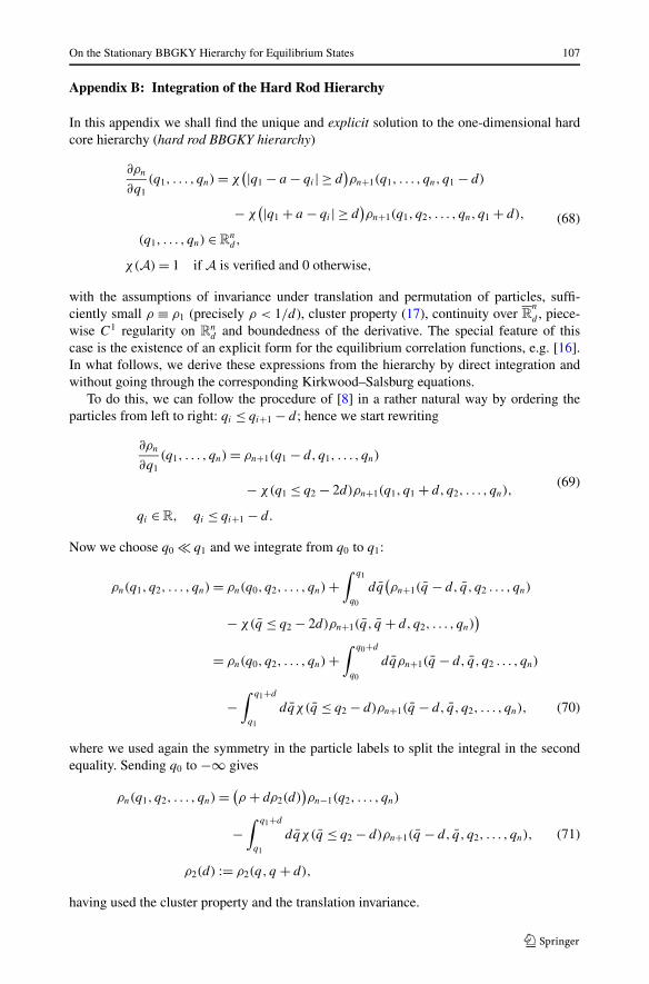
Appendix B: Integration of the Hard Rod Hierarchy

In this appendix we shall find the unique and explicit solution to the one-dimensional hardcore hierarchy (hard rod BBGKY hierarchy)

∂ρn

∂q1(q1, . . . , qn) = χ

(|q1 − a − qi | ≥ d)ρn+1(q1, . . . , qn, q1 − d)

− χ(|q1 + a − qi | ≥ d

)ρn+1(q1, q2, . . . , qn, q1 + d),

(q1, . . . , qn) ∈ Rnd,

χ(A) = 1 if A is verified and 0 otherwise,

(68)

with the assumptions of invariance under translation and permutation of particles, suffi-ciently small ρ ≡ ρ1 (precisely ρ < 1/d), cluster property (17), continuity over R

n

d , piece-wise C1 regularity on R

nd and boundedness of the derivative. The special feature of this

case is the existence of an explicit form for the equilibrium correlation functions, e.g. [16].In what follows, we derive these expressions from the hierarchy by direct integration andwithout going through the corresponding Kirkwood–Salsburg equations.

To do this, we can follow the procedure of [8] in a rather natural way by ordering theparticles from left to right: qi ≤ qi+1 − d ; hence we start rewriting

∂ρn

∂q1(q1, . . . , qn) = ρn+1(q1 − d, q1, . . . , qn)

− χ(q1 ≤ q2 − 2d)ρn+1(q1, q1 + d, q2, . . . , qn),

qi ∈ R, qi ≤ qi+1 − d.

(69)

Now we choose q0 � q1 and we integrate from q0 to q1:

ρn(q1, q2, . . . , qn) = ρn(q0, q2, . . . , qn) +∫ q1

q0

dq(ρn+1(q − d, q, q2 . . . , qn)

− χ(q ≤ q2 − 2d)ρn+1(q, q + d, q2, . . . , qn))

= ρn(q0, q2, . . . , qn) +∫ q0+d

q0

dqρn+1(q − d, q, q2 . . . , qn)

−∫ q1+d

q1

dqχ(q ≤ q2 − d)ρn+1(q − d, q, q2, . . . , qn), (70)

where we used again the symmetry in the particle labels to split the integral in the secondequality. Sending q0 to −∞ gives

ρn(q1, q2, . . . , qn) = (ρ + dρ2(d)

)ρn−1(q2, . . . , qn)

−∫ q1+d

q1

dqχ(q ≤ q2 − d)ρn+1(q − d, q, q2, . . . , qn),

ρ2(d) := ρ2(q, q + d),

(71)

having used the cluster property and the translation invariance.


Call R := ρ + dρ2(d). Iterating once the above equation we have

ρn(q1, q2, . . . , qn) = R

[

ρn−1(q2, . . . , qn) −∫ q1+d

q1

dqχ(q ≤ q2 − d)ρn(q, q2, . . . , qn)

]

.

(72)

We stress again that the above explained procedure does not lead directly to the Kirkwood–Salsburg equations. The extracted constant R is different from the activity of the hard rodgas (which is known to be given by z = ReRd , see for instance [16]). Nevertheless the set ofEq. (72) can be solved explicitly for every n, starting from n = 2 (the equation for n = 1 isof course useless in this model), as we show below. Actually, the simple structure of Eq. (72)allows to construct easily ρn from ρn−1: this structure is due to the strong symmetry used tosplit the integral in the second equality of (70), and it seems to have no analogue in higherdimensions.

We start with the n = 2 case. Call x = |q2 − q1|, x ≥ d . Formula (72) implies ρ2(d) =ρ2

1−ρd, R = ρ

1−ρdand

dρ2

dx(x) = −Rρ2(x), d < x < 2d,

dρ2

dx(x) = R

(−ρ2(x) + ρ2(x − a)), 2d < x.

(73)

Solving these set of equations iteratively in the intervals (kd, (k + 1)d), k = 1,2, . . . , usingthe continuity assumption, leads to

ρ2(x) = ρ

[x/d]∑

k=1

(ρ

1 − ρd

)k(x − kd)k−1

(k − 1)! e− (x−kd)ρ

1−ρd . (74)

In a similar way, using (72) and (74) and proceeding by induction on n, one finds that thesolution of (68) for n ≥ 2 is

ρn(q1, . . . , qn) = 1

ρn−2

n−1∏

j=1

ρ2(qj , qj+1). (75)

Appendix C: The Method of [8]

In this appendix we discuss the method established in [8] for the integration of the hierar-chy (15), pointing out an error in the formula for the activity and sketching how to correct it(we refer to [23] for details). At the end of the section we make comparisons between thismethod and the one established in the present paper.

We will need somewhat stronger assumptions than those of Theorem 1, namely the po-tential is a function ϕ ∈ C1(Rν) which is radial, stable and with compact support, whilethe smooth Maxwellian state has positional correlation functions ρn ∈ C1(Rνn)3 with thefollowing properties:

(a) ρn ≤ ξn, |∇qiρn| ≤ Cnξ

n, with ξ small enough;

3The assumptions on the smoothness of ϕ could be released as done in Sect. 2, by using Eqs. (11)–(13).


(b) ρn is translation and rotation invariant;(c) ρn satisfies an exponential strong cluster property, i.e.

∣∣ρT

n (q1, . . . , qn)∣∣ ≤ (Cξ)ne−κ|q1−qn|, C, κ > 0, (76)

where the truncated correlation functions ρTn can be defined by

{ρT

2 (q1, q2) = ρ2(q1, q2) − ρ(q1)ρ(q2),

ρT3 (q1, q2, q3) = ρ3(q1, q2, q3) − ρ2(q1, q2)ρ(q3) − ρ(q1)ρ2(q2, q3) + ρ(q1)ρ(q2)ρ(q3),

etc. (see [5] and [8, page 279]).Let us start by integrating Eq. (15) along a straight line connecting q0 (arbitrary) to q1:

using the same notations introduced for (22), we have

ρn(q1, . . . , qn) = e−β(Wq1 (q2,...,qn)−Wq0 (q2,...,qn))ρn(q0, q2, . . . , qn)

+∫ q1

q0

dq1

∫

Rν

dy1∂(−βϕ(q1 − y1))

∂q1

· e−β(Wq1 (q2,...,qn)−Wq1 (q2,...,qn))ρn+1(q1, q2, . . . , qn, y1), (77)

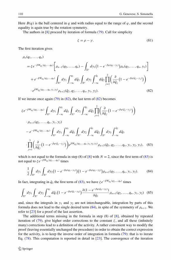
which is nothing but a rewriting of Eq. (22). In the assumption (b), the case n = 1 is a trivialidentity, hence we shall assume n ≥ 2 in the following.

The strategy consists in taking the limit as |q0| → +∞ right away, before iteration offormulas. This is also the essential difference with respect to the method discussed in Sect. 3,where such a limit is taken at the very end of the proof, after infinitely many iterations.Using (c), from (77) we get

ρn(q1, . . . , qn) = ρe−βWq1 (q2,...,qn)ρn−1(q2, . . . , qn)

+ e−βWq1 (q2,...,qn)

∫ q1

−∞dq1

∫

Rν

dy1∂(−βϕ(q1 − y1))

∂q1

· eβWq1 (q2,...,qn)ρn+1(q1, q2, . . . , qn, y1), (78)

where the double integral in the second term on the right hand side is well defined (by theexponential clustering (76) and the assumed rotation symmetry of the potential and of ρ2),though not absolutely convergent. Interchanging the integrations we find

ρn(q1, . . . , qn) = (ρ − γ )e−βWq1 (q2,...,qn)ρn−1(q2, . . . , qn)

+ e−βWq1 (q2,...,qn)

∫

Rν

dy1

∫ q1

−∞dq1

∂(−βϕ(q1 − y1))

∂q1

· eβWq1 (q2,...,qn)ρn+1(q1, q2, . . . , qn, y1), (79)

where we put

γ =∫

Rν

dy1

∫ q1

−∞dq1ρ2(q1, y1)

∂(−βϕ(q1 − y1))

∂q1

≡∫

B(q1)

dy1

∫ q1

−∞dq1ρ2(q1, y1)

∂(−βϕ(q1 − y1))

∂q1. (80)


Here B(q) is the ball centered in q and with radius equal to the range of ϕ, and the secondequality is again true by the rotation symmetry.

The authors in [8] proceed by iteration of formula (79). Call for simplicity

ζ = ρ − γ. (81)

The first iteration gives

ρn(q1, . . . , qn)

= ζe−βWq1 (q2,...,qn)

[

ρn−1(q2, . . . , qn) −∫

Rν

dy1

(1 − e−βϕ(q1−y1)

)ρn(q2, . . . , qn, y1)

]

+ e−βWq1 (q2,...,qn)

∫

Rν

dy1

∫ q1

−∞dq1

∫

Rν

dy2

∫ q1

−∞dq2

2∏

j=1

(∂

∂qj

(1 − e−βϕ(qj −yj )

))

· eβWq2 (q2,...,qn,y1,y2)ρn+2(q2, q2, . . . , qn, y1, y2). (82)

If we iterate once again (79) in (82), the last term of (82) becomes

ζe−βWq1 (q2,...,qn)

∫

Rν

dy1

∫ q1

−∞dq1

∫

Rν

dy2

∫ q1

−∞dq2

2∏

j=1

(∂

∂qj

(1 − e−βϕ(qj −yj )

))

· ρn+1(q2, . . . , qn, y1, y2)

− e−βWq1 (q2,...,qn)

∫

Rν

dy1

∫ q1

−∞dq1

∫

Rν

dy2

∫ q1

−∞dq2

∫

Rν

dy3

∫ q2

−∞dq3

·3∏

j=1

(∂

∂qj

(1 − e−βϕ(qj −yj )

))

eβWq3 (q2,...,qn,y1,y2,y3)ρn+3(q3, q2, . . . , qn, y1, y2, y3), (83)

which is not equal to the formula in step (8) of [8] with N = 2, since the first term of (83) isnot equal to ζe−βWq1 (q2,...,qn) times

1

2

∫

Rν

dy1

∫

Rν

dy2

(1 − e−βϕ(q1−y1)

)(1 − e−βϕ(q1−y2)

)ρn+1(q2, . . . , qn, y1, y2). (84)

In fact, integrating in q2 the first term of (83), we have ζe−βWq1 (q2,...,qn) times

∫

Rν

dy1

∫

Rν

dy2

∫ q1

−∞dq1

(1 − e−βϕ(q1−y2)

)∂(1 − e−βϕ(q1−y1))

∂q1ρn+1(q2, . . . , qn, y1, y2) (85)

and, since the integrals in y1 and y2 are not interchangeable, integration by parts of thisformula does not lead to the single desired term (84), in spite of the symmetry of ρn+1. Werefer to [23] for a proof of the last assertion.

The additional terms missing in the formula in step (8) of [8], obtained by repeatediteration of (79), give higher order corrections to the constant ζ , and all these (infinitelymany) corrections lead to a definition of the activity. A rather convenient way to modify theproof (leaving essentially unchanged the procedure) in order to obtain the correct expressionfor the activity, is to keep the inverse order of integration in formula (79): that is to iterateEq. (78). This computation is reported in detail in [23]. The convergence of the iteration


procedure is handled in assumptions (a), (b) and (c): after N iterations one gets a remainderRn,N that can be bounded as

∣∣Rn,N(q1, . . . , qn)

∣∣ ≤ (Aξ)n+N+1, (86)

where A is a suitable constant depending on β,C,κ,ϕ and the configuration q1, . . . , qn (butnot on ξ ), so that it goes to zero when N → ∞ if ξ is small enough. For these values of ξ , themethod provides convergence to the Kirkwood–Salsburg equations with exponential rate.

Comparisons We have the following differences with respect to the method presented inSect. 3:

1. The rate of convergence of the iteration is exponential, Eq. (86) (instead of factorial, seeEq. (27)): this implies convergence for sufficiently small values of ξ .

2. The radius of convergence of the procedure is at least 1/A, where A is not uniformlybounded in the maximum of the potential; a bound which is uniform in the hard corelimit could be obtained by assuming estimates for the smooth state as those in (12)–(13),instead of (a) of (76).

3. The exponential strong cluster property (76) (instead of the weak cluster (17)), as well asthe short range assumption on the potential (instead of the weak decrease (3)), are neededto control the convergence of the integrals over the unbounded domains of integration;

4. the same can be said for the assumption (b) in (76), that is for the rotation invariance ofthe state, which is not needed in Theorem 1. Furthermore we shall notice that, in the proofof Theorem 1, translation invariance is only used in the very last step, i.e. to perform thelimit |q0| → +∞ of expression (28), obtained after infinitely many iterations. This makesthe method suitable to extend the result to situations in which there is no symmetry anddifferent kinds of boundary condition are considered; an example of such a situation hasbeen given in Theorem 2.

References

1. Aizenman, M., Goldstein, S., Gruber, C., Lebowitz, J.L., Martin, P.: On the equivalence between KMS-states and equilibrium states for classical systems. Commun. Math. Phys. 53, 209–220 (1977)

2. Bogolyubov, N.N.: Problemy Dinamicheskoi Teorii ν Statisticheskoi Fizike, vol. 13, p. 196. Gostekhiz-dat, Moscow, Leningrad (1946)

3. Cercignani, C.: Theory and Application of the Boltzmann Equation. Scottish Academic, Edinburgh,London (1975)

4. Cohen, E.G.D.: The kinetic theory of dilute gases. In: Hanley, H.J.M. (ed.) Transport Phenomena inFluids, pp. 119–155 (1969)

5. Duneau, M., Iagolnitzer, D., Souillard, B.: Strong cluster properties for classical systems with finiterange interaction. Commun. Math. Phys. 35, 307–320 (1974)

6. Gallavotti, G.: On the mechanical equilibrium equations. Nuovo Cimento B 57, 208–211 (1968)7. Gallavotti, G.: Statistical Mechanics. A Short Treatise. Springer, Berlin (2000)8. Gallavotti, G., Verboven, E.: On the classical KMS boundary condition. Nuovo Cimento B 28, 274–286

(1975)9. Groeneveld, J.: Two theorems on classical many particles systems. Phys. Lett. 3, 50–51 (1962)

10. Gurevich, B.M., Suhov, Ju.M.: Stationary solutions of the Bogoliubov hierarchy equations in classicalstatistical mechanics. 1. Commun. Math. Phys. 49, 307–320 (1976)





14. Illner, R., Pulvirenti, M.: A derivation of the BBGKY-hierarchy for hard spheres particle systems. Transp.Theory Stat. Phys. 16, 997–1012 (1985)

15. Lebowitz, J.L.: Stationary nonequilibrium Gibbsian ensembles. Phys. Rev. 114, 5 (1959)16. Lieb, E.H., Mattis, D.C.: Mathematical Physics in One Dimension. Academic Press, New York (1966)17. Morrey, C.B.: On the derivation of the equation of hydrodynamics from statistical mechanics. Commun.

Pure Appl. Math. 8, 279–326 (1955)18. Penrose, O.: Convergence of fugacity expansions for fluids and lattice gases. J. Math. Phys. 4, 1312–1320

(1963)19. Penrose, O.: The remainder in Mayer’s fugacity series. J. Math. Phys. 4(12), 1488–1494 (1963)20. Ruelle, D.: Correlation functions of classical gases. Ann. Phys. 25, 109–120 (1963)21. Ruelle, D.: States of classical statistical mechanics. J. Math. Phys. 8, 1657–1668 (1962)22. Ruelle, D.: Statistical Mechanics. Rigorous Results. Benjamin, New York (1969)23. Simonella, S.: BBGKY hierarchy for hard sphere systems, Ph.D. dissertation. Sapienza University of

Rome (2011). Sect. 7.3 and Appendix D

Date post:	25-Aug-2016
Category:	Documents
Upload:	sergio
View:	214 times
Download:	2 times

On the Stationary BBGKY Hierarchy for Equilibrium States

Documents