UNIVERSIDAD AUTONOMA ´ FACULTAD DE CIENCIAS DEPARTAMENTO DE MATEM ´ ATICAS On the Theory and Practice of Variable Selection for Functional Data Jos´ e Luis Torrecilla Noguerales A dissertation submitted in partial fulfillment of the requirements for the Degree of Doctor of Mathematics Under the supervision of Jos´ e Ram ´ on Berrendero D´ ıaz and Antonio Cuevas Gonz´ alez Madrid, 2015
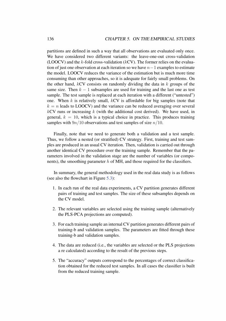
Transcript
UNIVERSIDAD AUTONOMA´
FACULTAD DE CIENCIASDEPARTAMENTO DE MATEMATICAS
On the Theory and Practice of VariableSelection for Functional Data
Jose Luis Torrecilla Noguerales
A dissertation submitted in partial fulfillment of the requirements for the Degreeof Doctor of Mathematics
Under the supervision of
Jose Ramon Berrendero Dıaz and Antonio Cuevas Gonzalez
Madrid, 2015
Agradecimientos
Este trabajo no serıa lo que es, y quiza ni siquiera serıa, sin la participacion demucha gente que ha contribuido de alguna manera, incluso sin saberlo, a que estatesis cobrase forma. A todas estas personas mi gratitud.
En primer lugar quiero expresar mi mas sincero agradecimiento a mis directo-res Jose Ramon y Antonio, sin los cuales esta tesis no existirıa. Gracias por darmela oportunidad de comenzar este proyecto y por haberme acompanado y apoyadoen cada etapa. Gracias tambien por vuestra confianza, motivacion y disponibi-lidad, sobre todo en los momentos complicados. Me siento muy afortunado dehaberos tenido como tutores, de vosotros he aprendido mucho mas que estadısti-ca.
Este agradecimiento es extensivo a Tati, Begona, Raimundo, Mari Paz, Emilio,Jose Ramon y a todos los profesores que tanto me han ensenado en mi paso porel C.P. Badiel, el I.E.S. Liceo Caracense y la Universidad Autonoma de Madrid.Y tambien a Luisfer y a Samuel que, aunque nunca me evaluaron, me ensenaronvaliosas lecciones y confiaron en mı para empezar a trabajar con chavales.
Mi agradecimiento a Ignasi Barba y David Garcıa-Dorado. Algunos de losresultados de esta tesis son fruto de la colaboracion con su grupo de investigacionen el Hospital Universitari Vall d’Hebron. Tambien quiero agradecerle a Jane-LingWang la oportunidad de trabajar con ella y su grupo en la UC Davis, y a Christinael hacer de Davis un lugar tan acogedor.
Durante todos estos anos en la UAM he tenido la suerte de contar con muchosbuenos companeros con los que discutir de matematicas, compartir las dificulta-des del doctorado, o simplemente pasar un buen rato y recobrar el animo paraenfrentarme a la tesis. Gracias a todos. En este punto me gustarıa agradecerlesexpresamente a Alberto, Alessandro y Bego el buen ambiente que ha habido en eldespacho y su ayuda, a Rocıo todas las conversaciones en esas largas horas de treny a Angela, Dani, Gema, Jaime, Jose, Mariaje, Raul, Sergio y Sofıa, el apoyo y elcompanerismo en distintos momentos. Y un agradecimiento especial para Carlos,que me aguanto durante toda la carrera con infinita paciencia, y para Carlos M.,
I
II AGRADECIMIENTOS
que le tomo el relevo en el master y que, junto con Angela, han sido importantesasesores sobre algunos aspectos de este trabajo.
No puedo olvidarme del Departamento de Matematicas, el Instituto de Inge-nierıa del Conocimiento y al programa FPI del MICINN, que pusieron los mediospara que pudiera llevar a cabo mi investigacion.
Tambien quiero dar las gracias a mis amigos de Guadalajara y a la gente delCentro Juvenil que han seguido la evolucion de esta tesis, aun no entendiendo lamayor parte de lo que les contaba, y han soportardo mis altibajos.
Gracias a Iris por apoyarme incondicionalmente y confiar tanto en mı, creyen-do muchas veces mas en mı que yo mismo. Gracias por conseguir sacarme unasonrisa incluso en los peores dıas y por escuchar una y mil veces todas esas cosasincomprensibles. Espero que la seleccion de variables o la clasificacion funcionalya no sean ideas tan extranas.
Quiero acabar dando las gracias a mi familia, a mis abuelos, a mi hermano Mi-guel Angel (corrector de estilo ocasional) y especialmente a mis padres Natividady Vıctor, a quienes esta tesis esta dedicada. Gracias por vuestro amor y sacrificios,sin vuestro apoyo nada de esto hubiera sido posible.
Abstract
Functional Data Analysis (FDA) might be seen as a partial aspect of the modern mainstreamparadigm generally known as Big Data Analysis. The study of functional data requires newmethodologies that take into account their special features (e.g. infinite dimension and highlevel of redundancy). Hence, the use of variable selection methods appears as a particularlyappealing choice in this context. Throughout this work, variable selection is considered in thesetting of supervised binary classification with functional data X(t), t ∈ [0, 1]. By variableselection we mean any dimension-reduction method which leads to replace the whole trajectoryX(t), t ∈ [0, 1], with a low-dimensional vector (X(t1), . . . , X(td)) still keeping a similar clas-sification error. In this thesis we have addressed the “functional variable selection” in classificationproblems from both theoretical and empirical perspectives.
We first restrict ourselves to the standard situation in which our functional data are gener-ated from Gaussian processes, with distributions P0 and P1 in both populations under study. Theclassical Hajek-Feldman dichotomy establishes that P0 and P1 are either mutually absolutely con-tinuous with respect to each other (so there is a Radon-Nikodym (RN) density for each measurewith respect to the other one) or mutually singular. Unlike the case of finite dimensional Gaus-sian measures, there are non-trivial examples of mutually singular distributions when dealing withGaussian stochastic processes. This work provides explicit expressions for the optimal (Bayes)rule in several relevant problems of supervised binary (functional) classification under the abso-lutely continuous case. Our approach relies on some classical results in the theory of stochasticprocesses where the so-called Reproducing Kernel Hilbert Spaces (RKHS) play a special role.This RKHS framework allows us also to give an interpretation, in terms of mutual singularity, forthe “near perfect classification” phenomenon described by Delaigle and Hall (2012a). We showthat the asymptotically optimal rule proposed by these authors can be identified with the sequenceof optimal rules for an approximating sequence of classification problems in the absolutely con-tinuous case.
The methodological contributions of this thesis are centred in three variable selection methods.The obvious general criterion for variable selection is to choose the “most representative” or “mostrelevant” variables. However, it is also clear that a purely relevance-oriented criterion could leadto select many redundant variables. First, we provide a new model-based method for variableselection in binary classification problems, which arises in a very natural way from the explicitknowledge of the RN-derivatives and the underlying RKHS structure. As a consequence, theoptimal classifier in a wide class of functional classification problems can be expressed in termsof a classical, linear finite-dimensional Fisher rule.
Our second proposal for variable selection is based on the idea of selecting the local maxima(t1, . . . , td) of the function V2
X(t) = V2(X(t), Y ), where V denotes the distance covariance
III
IV ABSTRACT
association measure for random variables due to Szekely et al. (2007). This method provides asimple natural way to deal with the relevance vs. redundancy trade-off which typically appearsin variable selection. This proposal is backed by a result of consistent estimation for the maximaof V2
X . We also show different models for the underlying process X(t) under which the relevantinformation is concentrated on the maxima of V2
X .
Our third proposal for variable selection consists of a new version of the minimum Redun-dancy Maximum Relevance (mRMR) procedure proposed by Ding and Peng (2005) and Penget al. (2005). It is an algorithm to systematically perform variable selection, achieving a reason-able trade-off between relevance and redundancy. In its original form, this procedure is based onthe use of the so-called mutual information criterion to assess relevance and redundancy. Keep-ing the focus on functional data problems, we propose here a modified version of the mRMRmethod, obtained by replacing the mutual information by the new distance correlation measure inthe general implementation of this method.
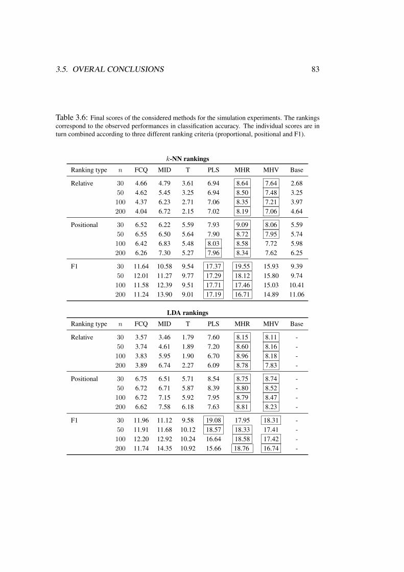
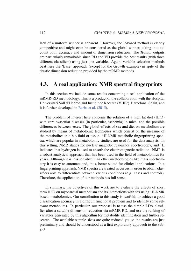
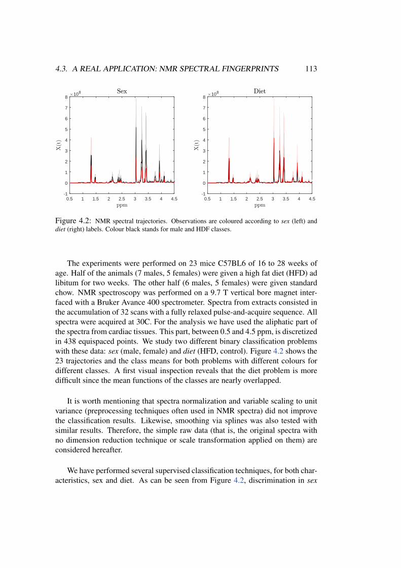
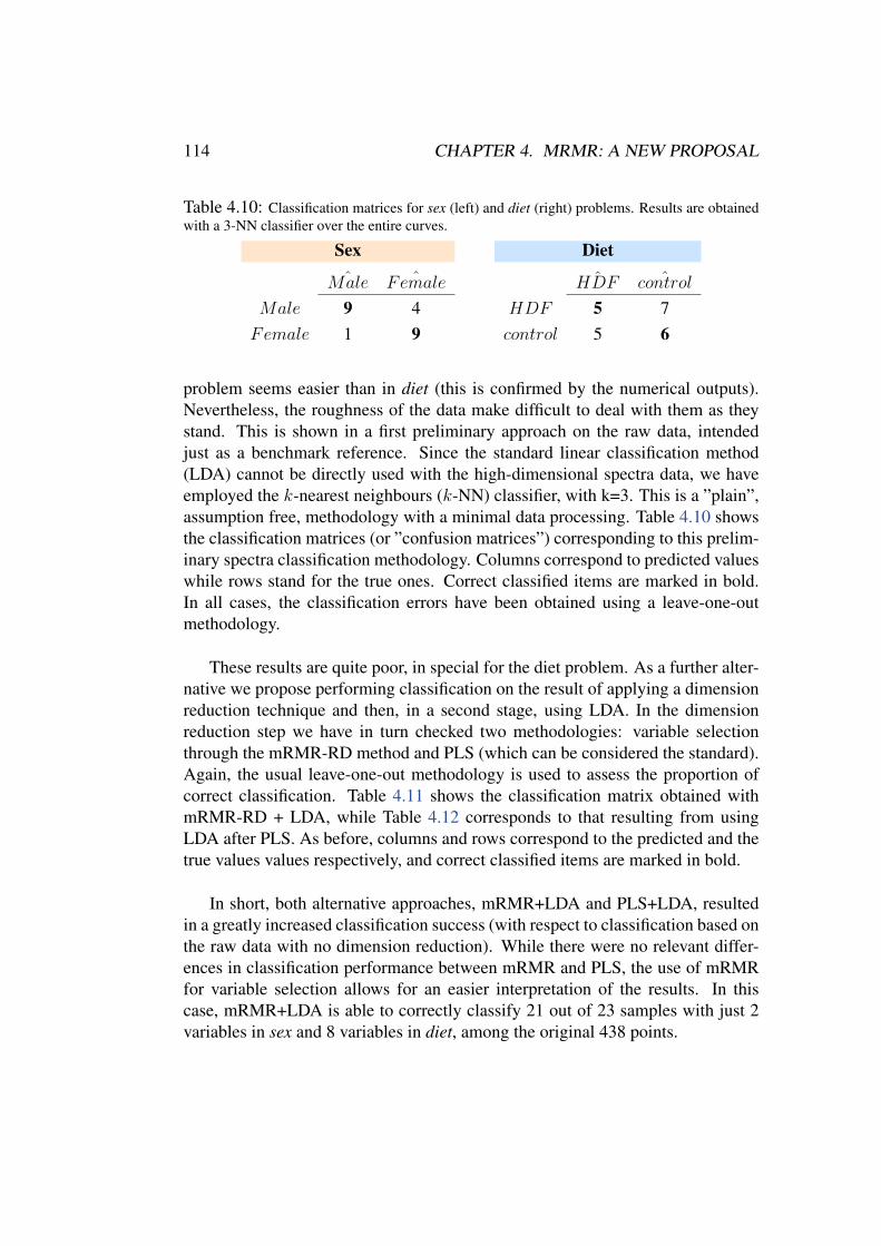
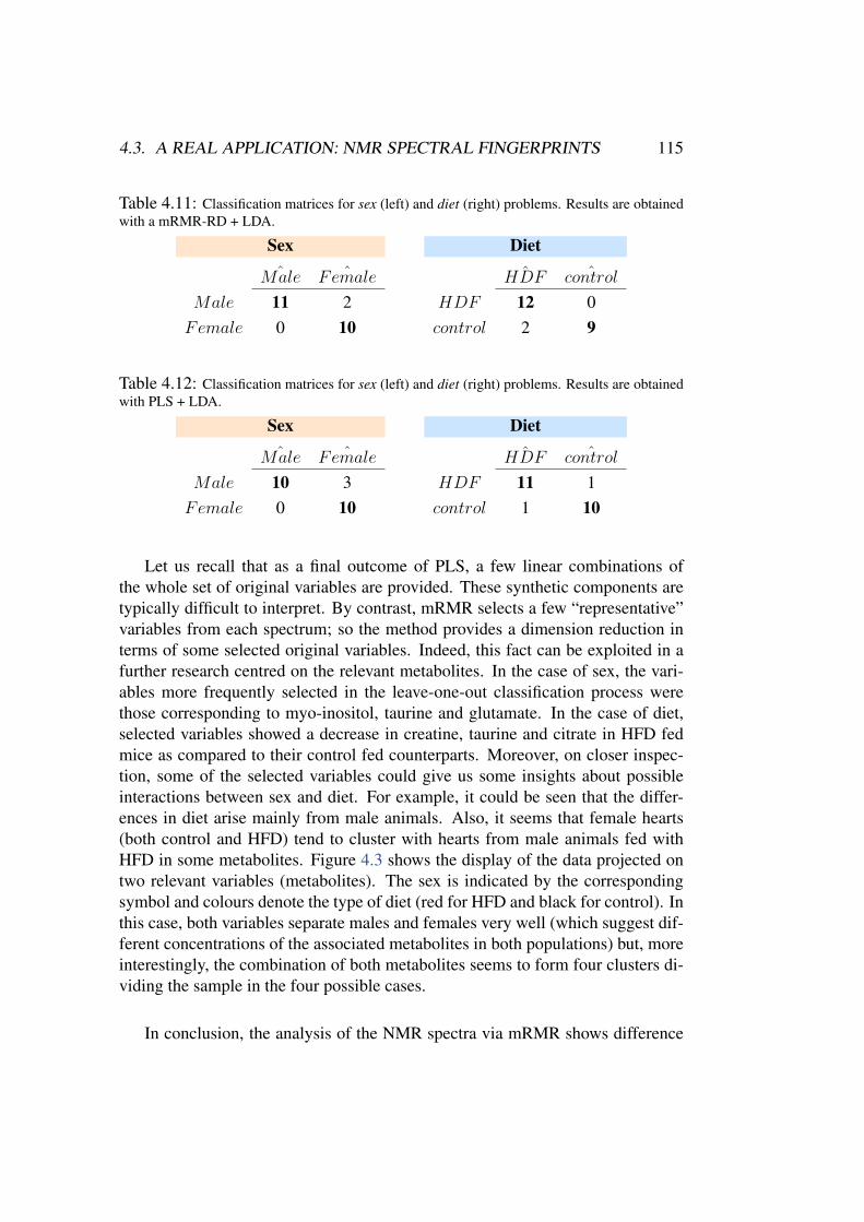
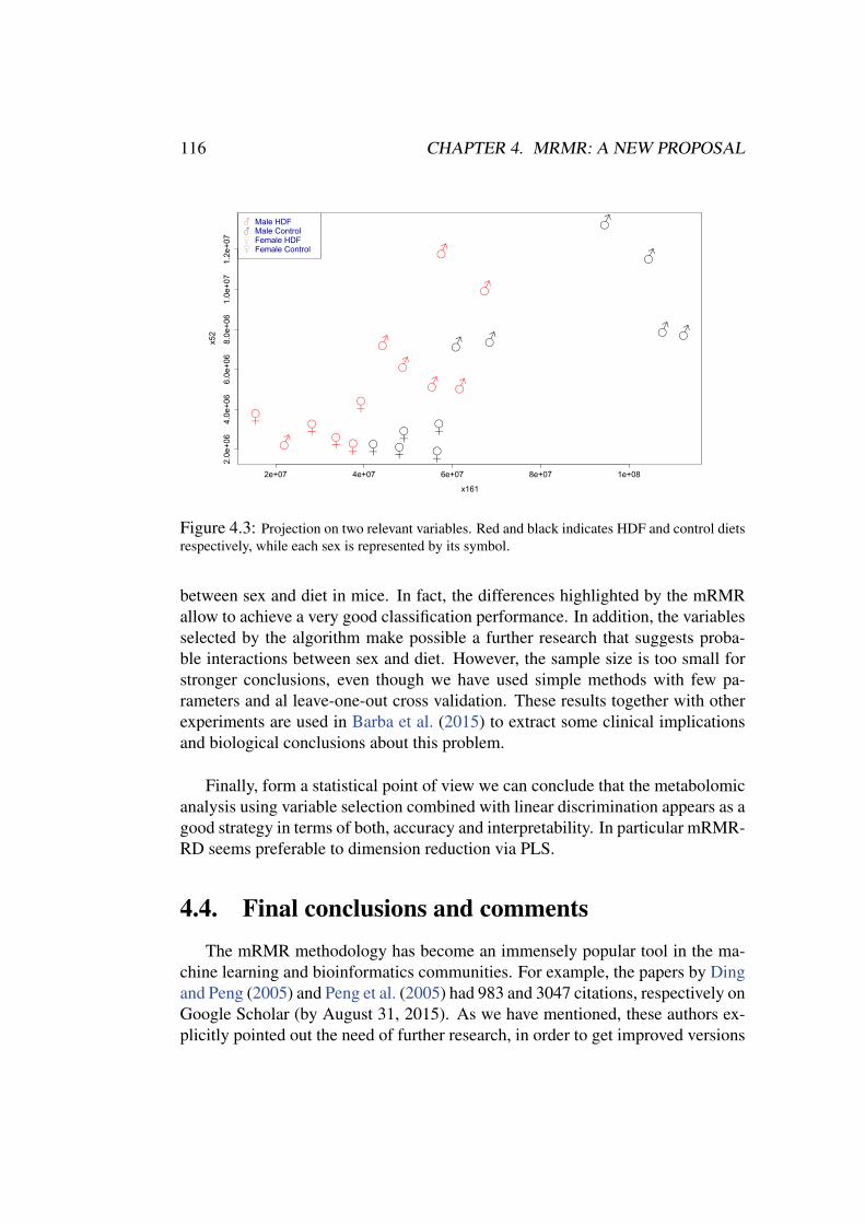
The performance of the new proposals is assessed through an extensive empirical study, in-cluding about 400 simulated models (100 functional models × 4 sample sizes) and real data ex-amples, aimed at comparing our variable selection methods with other standard procedures fordimension reduction. The comparison involves different classifiers. A real problem with biomed-ical data is also analysed in collaboration with researchers of Hospital Vall d’Hebron (Barcelona).The overall conclusions of the empirical experiments are quite positive in favour of the proposedmethodologies.
Resumen
El Analisis de Datos Funcionales (FDA por sus siglas en ingles) puede ser visto como unade las facetas del paradigma general conocido como Big Data Analysis. El estudio de los datosfuncionales requiere la utilizacion de nuevas metodologıas que tengan en cuenta las caracterısti-cas especiales de estos datos (por ejemplo, la dimension infinita y la elevada redundancia). Eneste contexto, las tecnicas de seleccion de variables parecen particularmente atractivas. A lo lar-go de este trabajo, estudiaremos la seleccion de variables dentro del marco de la clasificacionsupervisada binaria con datos funcionales X(t), t ∈ [0, 1]. Por seleccion de variables entende-mos cualquier metodo de reduccion de dimension enfocado a remplazar las trayectorias completasX(t), t ∈ [0, 1] por vectores de baja dimension (X(t1), . . . , X(td)) conservando la informa-cion discriminante. En esta tesis hemos abordado la “seleccion de variables funcional” en proble-mas de clasificacion tanto en su vertiente teorica como empırica.
Nos restringiremos esencialmente al caso general en que los datos funcionales estan generadospor procesos Gaussianos, con distribuciones P0 y P1 en las distintas poblaciones. La dicotomıade Hajek-Feldman establece que P0 y P1 solo pueden ser mutuamente absolutamente continuas(existiendo entonces una densidad de Radon-Nikodym (RN) de cada medida con respecto al aotra) o mutuamente singulares. A diferencia del caso finito dimensional, cuando trabajamos conprocesos Gaussianos aparecen ejemplos no triviales de distribuciones mutuamente singulares. Eneste trabajo se dan expresiones explıcitas de la regla de clasificacion optima (Bayes) para algunosproblemas funcionales binarios relevantes en el contexto absolutamente continuo. Nuestro enfoquese basa en algunos resultados clasicos de la teorıa de procesos estocasticos, entre los que losEspacios de Hilbert de Nucleos Reproductores (RKHS) desempenan un papel fundamental. Estemarco RKHS nos permite tambien dar una interpretacion del fenomeno de la “clasificacion casiperfecta” descrito por Delaigle and Hall (2012a), en terminos de la singularidad mutua de lasdistribuciones.
Las contribuciones metodologicas de esta tesis se centran en tres metodos de seleccion devariables. El criterio mas obvio para seleccionar las variables serıa elegir aquellas “mas represen-tativas” o “mas relevantes”. Sin embargo, un criterio basado unicamente en la relevancia probable-mente conducirıa a la seleccion de muchas variables redundantes. En primer lugar, proponemosun nuevo metodo de seleccion de variables basado en modelo, que surge de manera natural delconocimiento de las derivadas RN y de la estructura RKHS subyacente. Como consecuencia, elclasificador optimo para una amplia clase de problemas de clasificacion funcional puede expresar-se en terminos de la regla lineal de Fisher finito dimensional.
Nuestra segunda propuesta para seleccion de variables se basa en la idea de seleccionar losmaximos locales (t1, . . . , td) de la funcion V2
X(t) = V2(X(t), Y ), donde V denota la covarianza
V
VI RESUMEN
de distancias, medida de asociacion entre variables aleatorias propuesta por Szekely et al. (2007).Este procedimiento se ocupa de manera natural del equilibrio entre relevancia y redundancia tıpicode la seleccion de variables. Esta propuesta esta respaldada por un resultado de consistencia en laestimacion de los maximos de V2
X . Ademas, se muestran distintos modelos de procesos subyacen-tes X(t) para los que la informacion relevante se concentra en los maximos de V2
X .
La tercera propuesta para seleccionar variables es una nueva version del metodo mRMR(mınima Redundancia Maxima Relevancia), propuesto en Ding and Peng (2005) y Peng et al.(2005). Este algoritmo realiza una seleccion de variables sistematica, consiguiendo un equilibriorelevancia-redundancia razonable. El procedimiento mRMR original se basa en la utilizacion dela informacion mutual para medir la relevancia y la redundancia. Manteniendo el problema fun-cional como referencia, se propone una nueva version de mRMR en la que la informacion mutuaes remplazada por la nueva correlacion de distancias.
El rendimiento de las nuevas propuestas es evaluado mediante extensos estudios empıricoscon el objetivo de comparar nuestros metodos de seleccion de variables con otros procedimientosde reduccion de dimension ya establecidos. Los experimentos incluyen 400 modelos de simulacion(100 modelos funcionales × 4 tamanos muestrales) y ejemplos con datos reales. La comparativaincluye distintos clasificadores. Ademas se ha analizado un problema real con datos biomedicosen colaboracion con investigadores del Hospital Vall d’Hebron (Barcelona). Los resultados delestudio son, en general, bastante positivos para los nuevos metodos.
Throughout this thesis, we will denote the whole stochastic process by X .Provided that no confusion is possible, its value at a generic point twill be denotedby X(t) or, when convenient, by Xt. The trajectories drawn from X are denotedby x. Y stands for the class label associated with X .
As usual, transposition and inversion are denoted by the superscripts > and−1 respectively, and f ′ stands for the derivative of a real function f . Likewise,X ′ corresponds to an independent copy of the random variable X , and empiricalestimators are denoted by either a “hat” or the subscript n. Non-standard operatorsare defined on their first use.
For the sake of readability, we include here a relation of the main abbreviationsand symbols used in this dissertation.
AbbreviationsB Standard Brownian motion.BB Brownian bridge.BT Brownian motion with a trend.
FC Fisher-Correlation criterion.FDA Functional Data Analysis.fMRI Functional Magnetic Resonance Imaging.FPCA Functional Principal Components Analysis.
XV
XVI Symbols
kCV k-fold cross-validation.k-NN k Nearest Neighbours.
LDA Linear Discriminant Analysis.LOOCV Leave-one-out cross-validation.
MH Maxima Hunting.MI Mutual Information.mRMR minimum Redundancy Maximum Relevance.
NB Naıve Bayes classifier.NIR Near infrared.NMR Nuclear Magnetic Resonance.
OU Ornstein-Uhlembeck process.
PCA Principal Coponent Analysis.PLS Partial Least Squares.
RK-C Reproducing Kernel Classifier.RK-VS Reproducing Kernel Variable Selection.RKB-C RK-C under a Brownian assumption.RKB-VS RK-VS under a Brownian assumption.RKHS Reproducing Kernel Hilbert Spaces.RN Radon-Nikodym.
SLLN Strong Law of Large Numbers.SVM Support Vector Machine.
SymbolsP0 P1 The measure P0 is absolutely continuous with respect to
P1.P0 ∼ P1 P0 and P1 are equivalent (P0 P1 and P1 P0).P0⊥P1 Both measures are mutually singular.〈f, g〉K Inner product in the space H(K) if f, g ∈ H(K). Oth-
erwise, the congruence defined in Remark (a) of Theorem2.2.
‖ · ‖K Norm in the spaceH(K).
C[a, b] Space of real continuous functions on [a, b] endowed withthe supremum norm.
Cov Standard covariance.
d Number of selected variables.D Dirichlet space defined in Subsection 2.1.2.
Symbols XVII
Dn Training sample.dP1(x)/dP0 Radon-Nikodym derivative of P1 with respect to P0.
E Mathematical expectation.ε(t) Noise process.η(x) Regression function η(x) = E(Y |X = x).
h Tunning parameter in the estimation of the local maxima.H(K) Hilbert space associated with K.
I Set of indices.I Indicator function.I(·, ·) Asociation measure between two random variables.
K(·, ·) Covariance operator.
L∗ Bayes error.Ln Empirical error.
m(t) Mean function.
n Sample size.N Dimension of the discretization grid.
Ω Sample space.
p P(Y = 1).P Probability measure.P0, P1 Distributions of the stochastic processes defining the “pop-
ulations” denoted also P0, P1.Φ Cumulative distribution function of the standard normal.Φm,k Peak-type functions defined in Section 3.3.
R Distance correlation.R2
X R2(X(t), Y ).
V Distance covariance.V2X V2(X(t), Y ).
Var Variance.
In our lust for measurement, we frequently measurethat which we can rather than that which we wish to mea-sure... and forget that there is a difference.
George Udny Yule
Not everything that can be counted counts, and noteverything that counts can be counted.
William Bruce Cameron
Chapter 1
Introduction
1.1. Functional Data AnalysisFunctional Data Analysis (FDA) is a small part of that huge topic in contem-
porary science and technology known as Big Data. More specifically, FDA deals(using mathematical and computational tools) with those problems involving theuse of data which are ”big” in the sense that they are recorded ”in continuoustime” so that they are in fact real functions. Functional data appear in many sig-nificant areas from medicine to economics, taking the form of electrocardiograms,functional magnetic resonance imaging, spectroscopy, biometric signals, paths inspace, climate time series or economics indexes. Thus, it seems clear that theproper collection and treatment of these data in order to obtain the best informa-tion from them is a fundamental task. Nevertheless, the functional nature of thedata makes many classical statistical approaches inappropriate or directly useless,so new approximations and methods are needed.
Since term FDA was probably first coined by Ramsay (1982), the boom ofwhat we mean today by functional data analysis is relatively recent, with no morethan two decades of history (since the available techniques did not allow the ad-equate registration and process of functional data before that time). But despiteits novelty, the high research activity in this area has produced a big amount ofadvances and associated bibliography. A full review of all FDA developmentto this days exceeds the scope of this thesis by far. However, a comprehensiveapproximation to the topics which are more closely related to our work (data rep-resentation, supervised classification and variable selection) is given in the nextsections in order to provide a framework for our research as clear and completeas possible. But first let us comment some basic and general references in theFDA literature that readers interested in this theme might find helpful, as well as
1
2 CHAPTER 1. INTRODUCTION
point out some of the main differences between the functional and the multivariatesettings.
The former monograph by Ramsay and Silverman (2005, 1st ed. in 1997) pro-vided the first collection of ideas and techniques for functional data analysis andhas had a major influence in this field ever since. In this practical-oriented bookthe attention is centred in the L2 space, and both smoothing techniques and basisrepresentation play a central role (a functional data is assumed to be a realizationof a smooth process). Some of these ideas are applied to real-data problems ofdifferent areas in Ramsay and Silverman (2002) and the computational details (inboth R and MATLAB languages) can be found in Graves et al. (2009). The originalR code was distributed by the authors in the fda package contributing to the in-creasing popularity of the FDA. From another point of view, the reference book byFerraty and Vieu (2006) presents a comprehensive (theoretical and practical) treat-ment of the nonparametric approach to functional classification, prediction andforecasting in the wider setting of complete normed (and semi-normed) spaces.In this nonparametric setting, the monograph by Bosq and Blanke (2008) pro-vides new mathematical tools for prediction problems with functional data with amajor emphasis on the theoretical aspects. On the other hand, the book by Horvathand Kokoszka (2012) centres on inferential methods and their applications withspecial attention to dependent functional data. Finally, the recent book by Hs-ing and Eubank (2015) is a first attempt of collecting the mathematical conceptswhich are relevant to the theoretical foundations of FDA. The selected topics in-clude Reproducing Kernel Hilbert Spaces (RKHS), factor analysis, regression anddiscriminant analysis.
The increasing interest in FDA is also revealed by the number of special issuesand overview papers devoted to these topics that have been published in differentjournals. Some recent statistical surveys cover essential themes such as regres-sion, classification, clustering and dimension reduction. For example, Cuevas(2014) provides a comprehensive survey on FDA theory and methods, and Wanget al. (2015) pays special attention to the functional regression problem includinginverse regression and nonlinear models. It is also worth mentioning the collectivebook by Ferraty and Romain (2011) in which each chapter is a survey of a differ-ent topic by different authors, and the last two chapters of Goldfarb et al. (2011),by Delsol et al. (2011) and Gonzalez-Manteiga and Vieu (2011). Finally, the ap-plications of FDA in specific fields are also covered in thematic overviews such asBurfield et al. (2015), in chemometrics, or Ullah and Finch (2013) in biomedicine,with a singular systematic style.
Finally, it is noteworthy that in this booming field of statistics with functional
1.1. FUNCTIONAL DATA ANALYSIS 3
data, the computational and numerical aspects, as well as the real data applica-tions, have had (understandably) a major role so far. However, the underlyingprobabilistic theory, connecting the models (i.e., the stochastic processes) whichgenerate the data is far less developed. As pointed out by Biau et al. (2015), “Cu-riously, despite a huge research activity in the field, few attempts have been madeto connect the area of functional data analysis with the theory of stochastic pro-cesses”. The present thesis can be seen as a contribution to partially fill this gapregarding the relevant supervised (binary) classification setting and the associateddimension reduction problem via variable selection.
1.1.1. Some basic notions and difficulties in FDAThe references mentioned above and many other works place FDA as an area
of interest with many potential applications. So it is time to define what a func-tional data is. We have said that functional data can be curves, images, surfacesor more complex structures, i.e., any observation living in a functional (infinitedimensional) space. In this way, Ferraty and Vieu (2006) defines a functionaldata x as an observation of a random variable X which takes values in a func-tional space F . This thesis focuses on the most common case of real functionsdefined in a bounded interval, which arises in a wide variety of situations: spec-trometry, genetics, medicine, economics, biometrics, etc. Therefore, we precisethe definition of functional data in terms of stochastic processes (this approach iffollowed, e.g., in Hsing and Eubank (2015)). Let (Ω,F , P) be a probability spaceand I⊆ R an index set, an stochastic process is a collection of random variablesX(ω, t) : ω ∈ Ω, t ∈ I where X(·, t) is an F-measurable function on Ω. Thena functional data is just a realization (often called “trajectory”) of a stochasticprocess for all t ∈ I. Provided that no confusion is possible, we will denote thewhole process by X . Its value at a generic point t will be denoted by X(t) or,when convenient, by Xt.
In the functional setting stochastic processes play the role of random variablesin classical statistics. Continuing with this analogy, Gaussian processes occupythe place of the normal distribution in Rn. A stochastic process is said to beGaussian if and only if, for all t1, . . . , tk ∈ I the k-dimensional random vector(X(t1), . . . , X(tk)) has a normal distribution. Like their multivariate counter-parts, the distribution of Gaussian processes are fully determined by the meanfunction and the covariance operator, although in the functional case the family ofGaussian processes is not a parametric model. These processes have many otherwell-studied and valuable properties that can be found in any standard reference(see for example Doob (1953)). We will focus on this “central” type of processesseveral times throughout this work with special attention to the Standard Brown-
4 CHAPTER 1. INTRODUCTION
0.0 0.2 0.4 0.6 0.8 1.0
−2
−1
01
wiener process
t
X(t
)
0.0 0.2 0.4 0.6 0.8 1.0
−2
−1
01
OU process
t
X(t
)
0.0 0.2 0.4 0.6 0.8 1.0
−2
−1
01
wiener process
t
X(t
)
0.0 0.2 0.4 0.6 0.8 1.0
−3
−2
−1
01
2
vexponential process
t
X(t
)
0.0 0.2 0.4 0.6 0.8 1.0
−1
01
2wiener process
t
X(t
)
0.0 0.2 0.4 0.6 0.8 1.0
−2
−1
01
2
OU process
t
X(t
)
0.0 0.2 0.4 0.6 0.8 1.0
−1
01
2Brownian motion
t
X(t
)
0.0 0.2 0.4 0.6 0.8 1.0
−2
−1
01
2
OU process
t
X(t
)
0.0 0.5 1.0 1.5 2.0
−2
−1
01
2Brownian motion
t
X(t
)
0.0 0.5 1.0 1.5 2.0
−2.
0−
1.0
0.0
1.0
OU process
t
X(t
)
0.0 0.5 1.0 1.5 2.0
−2
−1
01
23
Brownian motion
t
X(t
)
0.0 0.5 1.0 1.5 2.0
−2
−1
01
OU process
t
X(t
)
0.0 0.5 1.0 1.5 2.0
−3
−2
−1
01
23
Brownian motion
t
X(t
)
0.0 0.5 1.0 1.5 2.0
−2
−1
01
2
OU process
t
X(t
)
0.0 0.5 1.0 1.5 2.0 2.5 3.0
−3
−2
−1
01
23
Brownian motion
t
X(t
)
0.0 0.5 1.0 1.5 2.0 2.5 3.0
−3
−2
−1
01
OU process
t
X(t
)
0.0 0.5 1.0 1.5 2.0
−2
−1
01
23
Brownian motion
t
X(t
)
0.0 0.5 1.0 1.5 2.0
−3
−2
−1
01
23
OU process
t
X(t
)
0.0 0.5 1.0 1.5 2.0
−3
−2
−1
01
2Brownian motion
t
X(t
)
0.0 0.5 1.0 1.5 2.0
−2
−1
01
2
OU process
t
X(t
)
0.0 0.5 1.0 1.5 2.0
−4
−2
02
Brownian motion
t
X(t
)
0.0 0.5 1.0 1.5 2.0
−3
−2
−1
01
2
OU process
t
X(t
)
0.0 0.5 1.0 1.5 2.0
−2
−1
01
2Brownian motion
t
X(t
)
0.0 0.5 1.0 1.5 2.0
−2
−1
01
23
OU process
t
X(t
)
0.0 0.5 1.0 1.5 2.0
−3
−2
−1
01
23
Brownian motion
t
X(t
)
0.0 0.5 1.0 1.5 2.0
−2
−1
01
2
OU process
t
X(t
)
0 2 4 6 8 10
−6
−4
−2
02
46
Brownian motion
t
X(t
)
0 2 4 6 8 10
−1.
5−
0.5
0.5
1.5
OU process
t
X(t
)
0.0 0.5 1.0 1.5 2.0
−2
−1
01
23
Brownian motion
t
X(t
)
0.0 0.5 1.0 1.5 2.0
−2
−1
01
2
OU process
t
X(t
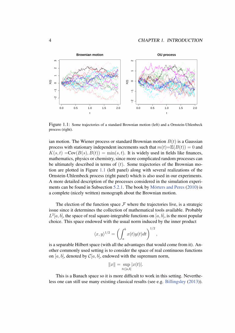
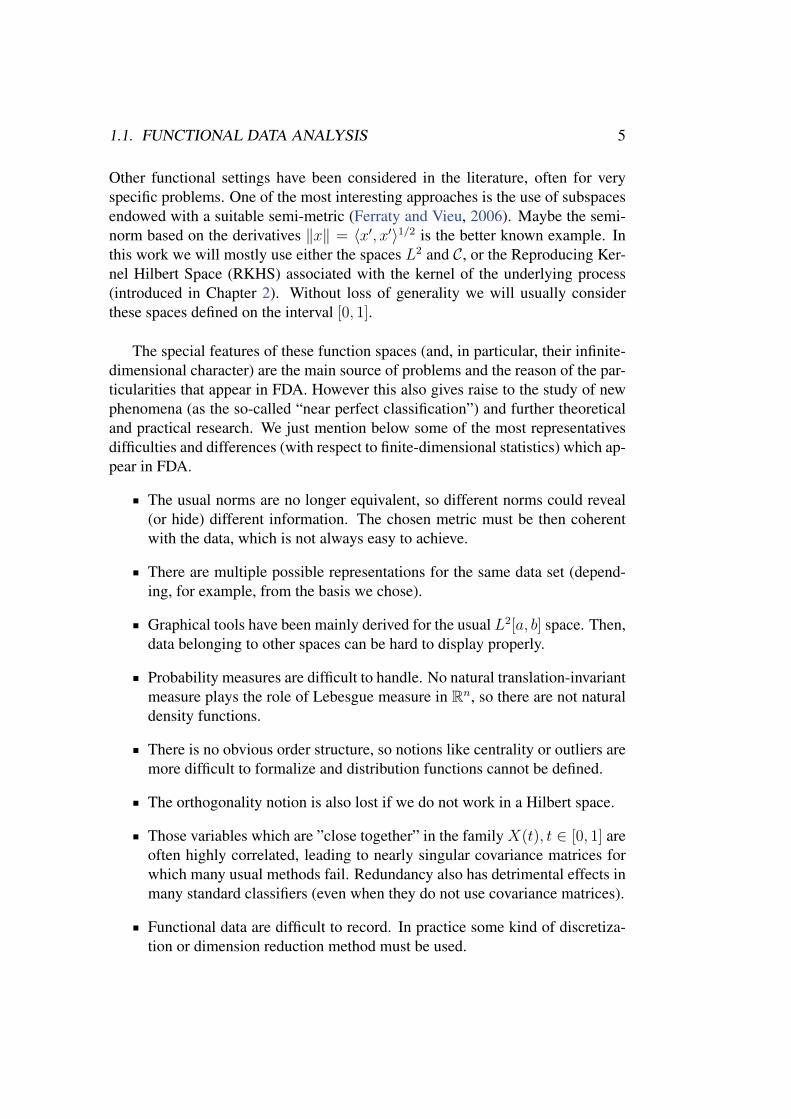
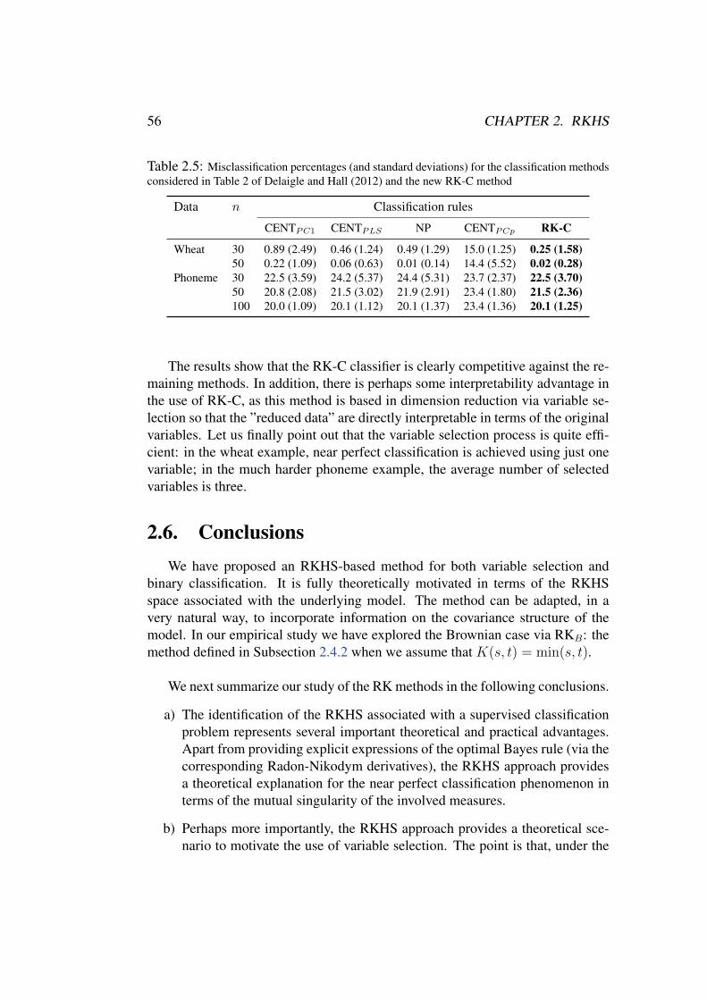
)Figure 1.1: Some trajectories of a standard Brownian motion (left) and a Ornstein-Uhlenbeckprocess (right).
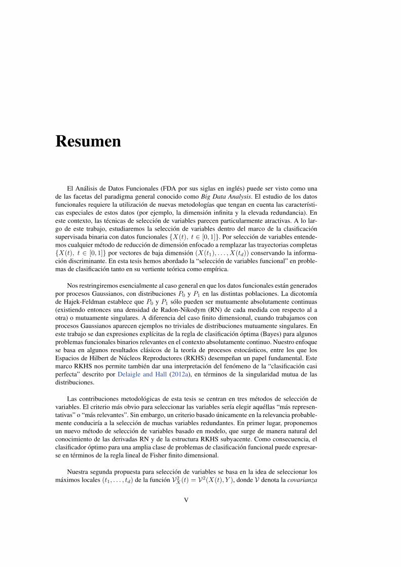
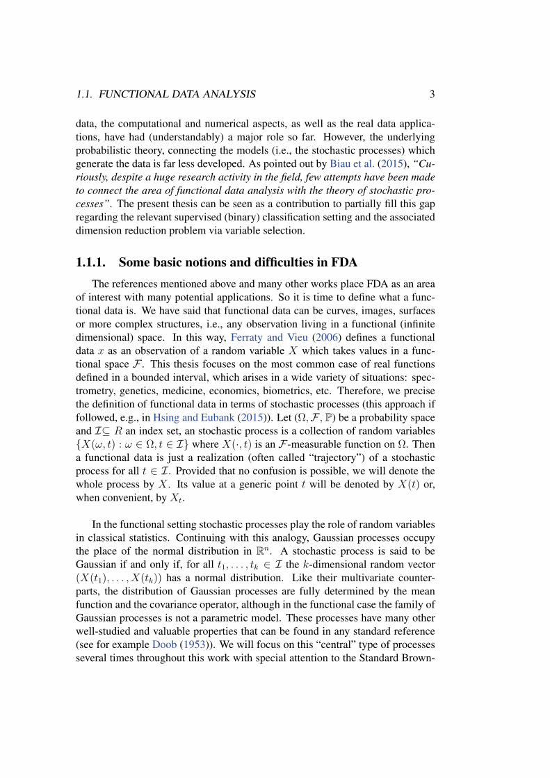
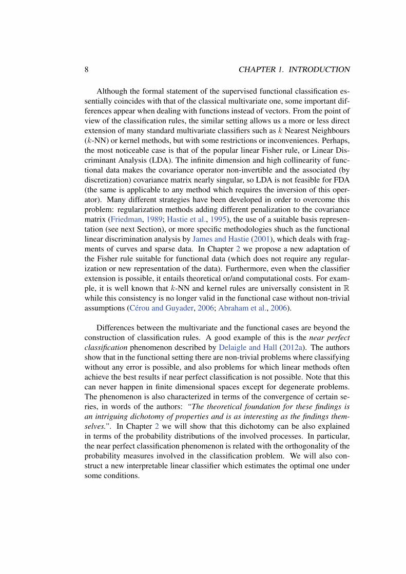
ian motion. The Wiener process or standard Brownian motion B(t) is a Gaussianprocess with stationary independent increments such that m(t)=E(B(t)) = 0 andK(s, t) =Cov(B(s), B(t)) = min(s, t). It is widely used in fields like finances,mathematics, physics or chemistry, since more complicated random processes canbe ultimately described in terms of (t). Some trajectories of the Brownian mo-tion are plotted in Figure 1.1 (left panel) along with several realizations of theOrnstein-Uhlembeck process (right panel) which is also used in our experiments.A more detailed description of the processes considered in the simulation experi-ments can be found in Subsection 5.2.1. The book by Morters and Peres (2010) isa complete (nicely written) monograph about the Brownian motion.
The election of the function space F where the trajectories live, is a strategicissue since it determines the collection of mathematical tools available. ProbablyL2[a, b], the space of real square-integrable functions on [a, b], is the most popularchoice. This space endowed with the usual norm induced by the inner product
〈x, y〉1/2 =
(∫ b
a
x(t)y(t)dt
)1/2
,
is a separable Hilbert space (with all the advantages that would come from it). An-other commonly used setting is to consider the space of real continuous functionson [a, b], denoted by C[a, b], endowed with the supremum norm,
‖x‖ = supt∈[a,b]
|x(t)|.
This is a Banach space so it is more difficult to work in this setting. Neverthe-less one can still use many existing classical results (see e.g. Billingsley (2013)).
1.1. FUNCTIONAL DATA ANALYSIS 5
Other functional settings have been considered in the literature, often for veryspecific problems. One of the most interesting approaches is the use of subspacesendowed with a suitable semi-metric (Ferraty and Vieu, 2006). Maybe the semi-norm based on the derivatives ‖x‖ = 〈x′, x′〉1/2 is the better known example. Inthis work we will mostly use either the spaces L2 and C, or the Reproducing Ker-nel Hilbert Space (RKHS) associated with the kernel of the underlying process(introduced in Chapter 2). Without loss of generality we will usually considerthese spaces defined on the interval [0, 1].
The special features of these function spaces (and, in particular, their infinite-dimensional character) are the main source of problems and the reason of the par-ticularities that appear in FDA. However this also gives raise to the study of newphenomena (as the so-called “near perfect classification”) and further theoreticaland practical research. We just mention below some of the most representativesdifficulties and differences (with respect to finite-dimensional statistics) which ap-pear in FDA.
The usual norms are no longer equivalent, so different norms could reveal(or hide) different information. The chosen metric must be then coherentwith the data, which is not always easy to achieve.
There are multiple possible representations for the same data set (depend-ing, for example, from the basis we chose).
Graphical tools have been mainly derived for the usual L2[a, b] space. Then,data belonging to other spaces can be hard to display properly.
Probability measures are difficult to handle. No natural translation-invariantmeasure plays the role of Lebesgue measure in Rn, so there are not naturaldensity functions.
There is no obvious order structure, so notions like centrality or outliers aremore difficult to formalize and distribution functions cannot be defined.
The orthogonality notion is also lost if we do not work in a Hilbert space.
Those variables which are ”close together” in the family X(t), t ∈ [0, 1] areoften highly correlated, leading to nearly singular covariance matrices forwhich many usual methods fail. Redundancy also has detrimental effects inmany standard classifiers (even when they do not use covariance matrices).
Functional data are difficult to record. In practice some kind of discretiza-tion or dimension reduction method must be used.
6 CHAPTER 1. INTRODUCTION
Function spaces are “difficult to fill”. This means that usually one needshuge sample sizes to get many functional data in a small neighbourhood ofa given function. As a consequence, non-parametric methods (which aretypically of “local” nature) have often slow convergence rates so that largesample sizes are needed.
Some of these points, specially those concerning the infinite dimensionality,redundancy between variables and representation issues, will be further developedin the next sections and chapters. We will also see the implications of choice ofthe space where the functional data are supposed to “live”.
1.2. Supervised ClassificationThe discrimination procedures (also called supervised classification methods
in modern terminology) are now a commonplace in the standard use of statistics.Their origins go back to the classical work by Fisher (1936), motivated by biolog-ical taxonomy problems. Today, biomedical sciences remain as a major field ofapplication of discrimination techniques but other areas, like engineering, providealso several important problems (signal theory, image analysis, speech recogni-tion...). The books by Devroye et al. (2013), Hastie et al. (2009) and Duda et al.(2012) offer insightful, complementary perspectives of this topic. In the rest ofthis thesis we will focus on the binary discrimination problem, even though manymethods and results can be immediately extended to the multiclass case.
While the statement and basic ideas behind the discrimination problem arewidely known, we need to briefly recall them for the sake of clarity. Supposethat an explanatory random variable X (say, e.g., the result of a medical analysis)taking values in a feature space F can be observed in the individuals of two pop-ulations P0 and P1 (e.g., P0 could be the population of healthy individuals and P1
that of people suffering from a certain illness). Let Y denote a binary random vari-able, with values in 0, 1, indicating the membership to P0 or P1. On the basisof a data set Dn= ((X1, Y1), . . . , (Xn, Yn)) of n independent observations drawnfrom (X, Y ), the discrimination problem aims at predicting the membership classY of a new observation for which only the variableX is known. In the medical ex-ample, the goal would be to classify a patient as healthy or ill from the observationof X , in view of the experience provided by the data base Dn of well-classifiedpatients (this accounts for the expression supervised classification).
A classifier or classification rule is just a measurable function g : F → 0, 1.It is natural to assess the performance of a classifier by the corresponding classi-
1.2. SUPERVISED CLASSIFICATION 7
fication error L = P(g(X) 6= Y ). It is well known that this classification error isminimized by the so-called Bayes classifier,
g∗(x) = Iη(x)>1/2, (1.1)
where η(x)= E(Y |X = x) = P(Y = 1|X = x). The corresponding minimal“classification error” (i.e., the misclassification probability) L∗= P(g∗(X) 6= Y )is called Bayes error. Since this optimal (Bayes) classifier is in general unknown,the purpose of (binary) supervised classification is just to construct data-drivenclassifiers gn: F → 0, 1, with gn(x;Dn) = gn(x), aimed at providing reason-able (in some sense) approximations of g∗. A common strategy is the so-calledplug–in approach, consisting in replacing η(x) with a suitable data-driven estima-tor. The goodness of these classifiers is assessed in relation with the Bayes error,in this sense a sequence of classifiers gn is weakly consistent if Ln→ L∗ inprobability as n→∞, and it is strong consistent if Ln → L∗ almost surely (a.s.)when n→∞.
Since the distribution of (X, Y ) is also unknown in general, the error associ-ated with a classifier gn is unknown too. However it can be easily estimated bythe empirical risk
Ln =1
n
n∑i=1
Ign(Xi)6=Yi.
This empirical risk (calculated over an independent test sample) is the usual crite-rion for comparison among different methods in our simulation experiments. Thiscan also be used to construct new classifiers with the only goal of minimizing thiserror. Similarly to wrapper methods described in Section 1.4, the idea lies in thegeneration of a range of classification rules and the election of that which mini-mizes the empirical risk. This methodology is supposed to produce, in general,more accurate but less general classifiers (in the sense that the minimization ofthis error is completely data-dependent) than the plug-in approach. Empirical-risk classifiers are also supposed to converge faster to the Bayes error, but it is acontroversial point (Audibert and Tsybakov, 2007).
1.2.1. Classification with functional dataThe general setup outlined before remains valid in the functional setting, but
here the feature space F will be an infinite-dimensional functional space. Typ-ical choices for F are F = L2[0, 1] and F = C[0, 1]. Thus, our data are oftype (X1, Y1), . . . , (Xn, Yn), where the Xi are iid trajectories in L2[0, 1] or C[0, 1],drawn from a stochastic process X = X(t) = X(ω, t).
8 CHAPTER 1. INTRODUCTION
Although the formal statement of the supervised functional classification es-sentially coincides with that of the classical multivariate one, some important dif-ferences appear when dealing with functions instead of vectors. From the point ofview of the classification rules, the similar setting allows us a more or less directextension of many standard multivariate classifiers such as k Nearest Neighbours(k-NN) or kernel methods, but with some restrictions or inconveniences. Perhaps,the most noticeable case is that of the popular linear Fisher rule, or Linear Dis-criminant Analysis (LDA). The infinite dimension and high collinearity of func-tional data makes the covariance operator non-invertible and the associated (bydiscretization) covariance matrix nearly singular, so LDA is not feasible for FDA(the same is applicable to any method which requires the inversion of this oper-ator). Many different strategies have been developed in order to overcome thisproblem: regularization methods adding different penalization to the covariancematrix (Friedman, 1989; Hastie et al., 1995), the use of a suitable basis represen-tation (see next Section), or more specific methodologies shuch as the functionallinear discrimination analysis by James and Hastie (2001), which deals with frag-ments of curves and sparse data. In Chapter 2 we propose a new adaptation ofthe Fisher rule suitable for functional data (which does not require any regular-ization or new representation of the data). Furthermore, even when the classifierextension is possible, it entails theoretical or/and computational costs. For exam-ple, it is well known that k-NN and kernel rules are universally consistent in Rwhile this consistency is no longer valid in the functional case without non-trivialassumptions (Cerou and Guyader, 2006; Abraham et al., 2006).
Differences between the multivariate and the functional cases are beyond theconstruction of classification rules. A good example of this is the near perfectclassification phenomenon described by Delaigle and Hall (2012a). The authorsshow that in the functional setting there are non-trivial problems where classifyingwithout any error is possible, and also problems for which linear methods oftenachieve the best results if near perfect classification is not possible. Note that thiscan never happen in finite dimensional spaces except for degenerate problems.The phenomenon is also characterized in terms of the convergence of certain se-ries, in words of the authors: “The theoretical foundation for these findings isan intriguing dichotomy of properties and is as interesting as the findings them-selves.”. In Chapter 2 we will show that this dichotomy can be also explainedin terms of the probability distributions of the involved processes. In particular,the near perfect classification phenomenon is related with the orthogonality of theprobability measures involved in the classification problem. We will also con-struct a new interpretable linear classifier which estimates the optimal one undersome conditions.
1.2. SUPERVISED CLASSIFICATION 9
Dozens of classifiers could be used according to the data under study, thegoals of the analysis, computational or time requirements, etc. Several functionalclassifiers have been considered in the literature; see, e.g., Baıllo et al. (2011) for asurvey. For other recent proposals see, for example,Cuesta-Albertos et al. (2015)and Martin-Barragan et al. (2014) . In addition, after a dimension reduction anymultivariate classifier is a valid choice (at least in principle). In this thesis, we areprimarily concerned with the comparison of several variable selection methodsunder the same conditions (on the more general possible way). Our goal is to getgood variable selection methods (working properly in a wide range of situations)rather than to get the best classification rate for a specific problem. For thesereasons, we have chosen a small number of popular and not too complex classifiersbut with good performance in practice, which are commonly used as benchmarksin the literature. In fact, we will see that some of these simple classifiers achievereally good results for different problems.
Maybe the simplest one is the so-called k nearest neighbours rule, accordingto which an observation x is assigned to P1 if and only if the majority amongthe k sample observations Xi nearest to x fulfil Yi = 1. In general, k-NN couldbe considered (from the limited experience so far available; see e.g., Baıllo et al.(2011); Dudoit et al. (2002)) a sort of benchmark, reference method for functionalsupervised classification. Simplicity, ease of motivation and general good per-formance (it typically does not lead to gross classification errors) are perhaps themost attractive features of this method.
Other, more recent, extremely popular classifier is the so-called Support VectorMachine (SVM); see Cortes and Vapnik (1995). These classifiers depend on aauxiliary function called “kernel”. The SVM classifier based on a linear kernelis particularly successful (see e.g. Dıaz-Uriarte and Alvarez de Andres (2006)or Gonen (2011)) and is probably the linear method of reference today. Thisreproducing kernel based methodology is often used for comparisons in referencewhere similar studies are carried out (Ding and Peng, 2005; Peng et al., 2005).
Finally, we will consider the popular Fisher’s linear classifier (LDA) usedoften in classical discriminant analysis. This is a well-known rule which is com-monly utilized as a reference because of its popularity, simplicity and good per-formance in many low-dimensional real problems (see, e.g. Hand (2006)). This isspecially recommended when distributions are Gaussian, which will be frequentin our context. However, note that LDA can be used only on the “reduced data”resulting from a dimension reduction method while k-NN and SVM can deal withthe entire data.
10 CHAPTER 1. INTRODUCTION
Other recurrent classifiers in similar studies were also considered but they arejust occasionally commented (or not included) in this dissertation for the sakeof clarity and concision. The results for these classifiers are nearly analogous tothose presented in this work and will be briefly commented in Chapter 5.
1.2.2. Supervised classification and absolute continuityAs we will comment below, the relationship between the probability measures
involved in the classification problem entails strong consequences regarding theoptimal rule and the optimal classification error. In fact, the absolute continuityor mutual singularity of these measures determine whether one can achieve a per-fect classification in some models or not, and Radon-Nikodym derivatives (in theabsolute continuous case) are related with the calculation of explicit expressionsfor the Bayes rules.
The expression P1P0 indicates that P1 is absolutely continuous with respectto P0 (i.e. P0(A) = 0 entails P1(A) = 0). Note that, from the Hajek-Feldman di-chotomy for Gaussian measures (Feldman, 1958), P1 P0 implies also P0 P1,so that both measures are in fact mutually absolutely continuous (or “equivalent”).This is often denoted by P0 ∼ P1.
When P0 and P1 are completely known in advance and P1 P0, the optimalclassification rule (often called Bayes rule) is
g∗(x) = Iη(x)>1/2 = I dP1(x)dP0
> 1−pp
, (1.2)
where I denotes the indicator function, η(x) = P(Y = 1|X = x) = E(Y |X =x), p= P(Y = 1) and dP1(x)/dP0 is the Radon-Nikodym derivative of P1 withrespect to P0; see (Baıllo et al., 2011, Thm. 1) for additional details.
If the Radon-Nikodym derivative dP1(x)/dP0 is explicitly known, there is notmuch else to be said. However, in practice, this is not usually the case. Even if thegeneral expression of dP1(x)/dP0 is known, it typically depends on the covarianceK(s, t) = Cov(X(s), X(t)) and mean functions mi(t) = E(X(t)|Y = i) of Pi,i = 1, 2.
As said above, the term “supervised” accounts for the fact that, in any case, adata set of “well-classified” independent observations Dn is assumed to be avail-able beforehand. Therefore, a common strategy is to use these data to estimatethe optimal rule (1.2). This plug–in approach is often implemented in a non-parametric way (e.g., estimating η(x) by a nearest-neighbour estimator) which
1.3. FUNCTIONAL DATA REPRESENTATION 11
does not require much information on the precise structure of η(x) or dP1(x)/dP0.However, in some other cases we have a quite precise information on the structureof dP1(x)/dP0, so that we can take advantage of this information to get betterplug-in estimators of g∗(x). This idea will be developed in Chapters 2 and 3.
1.3. Functional data representationIn this section we refer to the difficulties of FDA appearing during the data
preprocessing due to three principal causes: the choice of the functional spaceand representation of data, the infinite dimension of the observations and the datacollection procedure.
1.3.1. Smoothing and basis representationFrom a practical point of view, it is impossible to observe a complete func-
tional data. Nowadays, high-tech sensors allow for monitoring processes in finerand finer grids, but at the end some sort of discretization used. Therefore, whatwe have in practice is not the process X(t), t ∈ [0, T ] but a high-dimensionalvector (x(t1), . . . , x(tN)) in the discrete grid t1, . . . , tN . And this vector of highlycorrelated covariates represents the functional data. Indeed, we will often have acollection of n of these observations that is usually represented as a matrix with nfiles and N columns; this is the training sample or training set. A question to dis-cuss is whether these vectors are true functional data. In our opinion the answer isaffirmative: on the one hand, in some cases the grid can be as fine as desired so theprocess is virtually observable at any instant t. On the other hand, we can choosea functional model to approximate the data. So, the idea is that behind these vec-tors there are real functions with all the corresponding implications, or in wordsof Ramsay and Silverman (2005): “The term functional in reference to observeddata refers to the intrinsic structure of the data rather than to their explicit form”.
Furthermore, the presence of noise presents similar problems. In practice,most functional data are contaminated with random noise. This is also calledmeasurement error, although sometimes the source of noise will not be an errorin the measurement. Noise is usually modelled considering that we observe adata y(t) = X(t)+ε(t), where X(t) is a real function and ε(t) is random noiseindependent from X(t) such that E [ε(t)] = 0 and Varε(t) = σ2. These errors aresometimes insignificant, for example when recording the height of children alongtime, but in other cases noise is a critical point, as head movements when takingfMRI’s (functional magnetic resonance images).
12 CHAPTER 1. INTRODUCTION
The goal in both cases is obtaining the original function from the (noisy) ob-served vector, or sometimes, getting a smoother version for further actions, forexample to take derivatives. There are FDA tools that allow us to “recover” theoriginal function (or a very close approximation) from the observation or just geta smooth enough approximation. These methods are basically grouped in two bigfamilies: basis representation and smoothing.
The basis representation is a recurrent tool in functional data analysis. It playsthe double role of getting a continuous function and reducing the dimension bytruncating the expansion series. A full review of these topics can be found in(Ramsay and Silverman, 2005, ch. 3). Assuming that the data x(t) live in afunctional space F and let φi(t)N be a basis of that space, then x(t) can berepresented by the series x =
∑∞i=1 ciφi(t), where ci are the coefficients corre-
sponding to the basis. In practice, the infinite series is truncated at certain elementk and we approximate x(t) by x(t) =
∑ki=1 ciφi(t). This number k is a sort of
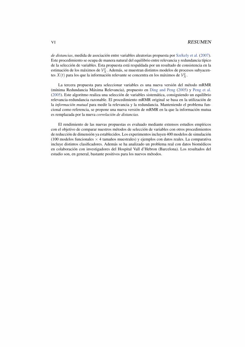
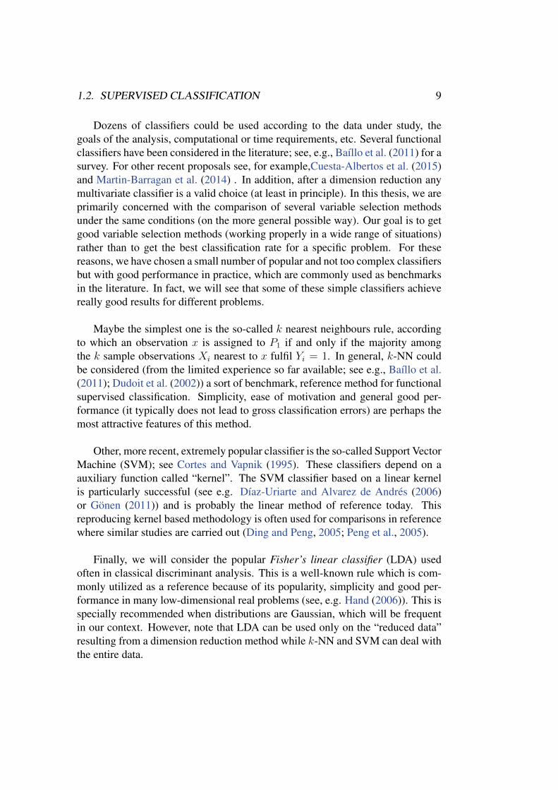
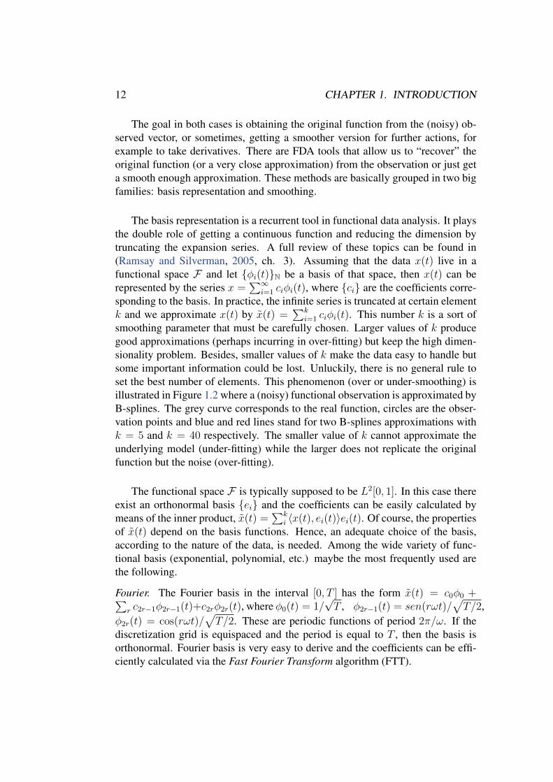
smoothing parameter that must be carefully chosen. Larger values of k producegood approximations (perhaps incurring in over-fitting) but keep the high dimen-sionality problem. Besides, smaller values of k make the data easy to handle butsome important information could be lost. Unluckily, there is no general rule toset the best number of elements. This phenomenon (over or under-smoothing) isillustrated in Figure 1.2 where a (noisy) functional observation is approximated byB-splines. The grey curve corresponds to the real function, circles are the obser-vation points and blue and red lines stand for two B-splines approximations withk = 5 and k = 40 respectively. The smaller value of k cannot approximate theunderlying model (under-fitting) while the larger does not replicate the originalfunction but the noise (over-fitting).
The functional space F is typically supposed to be L2[0, 1]. In this case thereexist an orthonormal basis ei and the coefficients can be easily calculated bymeans of the inner product, x(t) =
∑ki 〈x(t), ei(t)〉ei(t). Of course, the properties
of x(t) depend on the basis functions. Hence, an adequate choice of the basis,according to the nature of the data, is needed. Among the wide variety of func-tional basis (exponential, polynomial, etc.) maybe the most frequently used arethe following.
Fourier. The Fourier basis in the interval [0, T ] has the form x(t) = c0φ0 +∑r c2r−1φ2r−1(t)+c2rφ2r(t), where φ0(t) = 1/
√T , φ2r−1(t) = sen(rωt)/
√T/2,
φ2r(t) = cos(rωt)/√T/2. These are periodic functions of period 2π/ω. If the
discretization grid is equispaced and the period is equal to T , then the basis isorthonormal. Fourier basis is very easy to derive and the coefficients can be effi-ciently calculated via the Fast Fourier Transform algorithm (FTT).
1.3. FUNCTIONAL DATA REPRESENTATION 13
TrueObsv.k=5k=40k
Figure 1.2: Approximation of a functional data via B-splines. Grey: true data. Blue: under-fittedapproximation (k = 5). Red: over-fitted approximation (k = 40).
B-Splines. Splines basis might be the most popular basis nowadays (for non pe-riodical data). This basis combines the efficiency of polynomials (which are in-cluded in it) with a greater flexibility, so that it usually needs just a few elements.The technique basically lies on dividing the time interval and making a polynomialapproximation in each subinterval while taking care of the breakpoints. Manyvariants can be used for particular cases, see De Boor (1978) for some examples.We will use expansions of this type when taking derivatives in practice.
Wavelets. The idea behind this representation is that any function in L2 can beproperly approximated by suitable mother wavelet function ψ and its translationsand dilations of the form ψm,k(t) = 2m/2ψ(2mt− k), m, k ∈ N. The use of thesebasis is associated with treatment of signals since they can deal with discontinuousand nondifferentiable functions in a natural way, but now it is an extended practicealso in FDA (see e.g., Pigoli and Sangalli (2012); Antoniadis et al. (2013)). Insome examples of this thesis, the so-called Haar basis (formed by square pulses)will play a relevant role.
Empirical. Empirical bases are constructed from the data aiming at optimizingsome particular target. The most popular one is that obtained using FunctionalPrincipal Components Analysis. This is an extension of the multivariate func-tional data analysis through the Karhunen-Loeve expasion. This approach, whichtries to capture the variance of the data in the new representation, have beensuccessfully employed in many FDA techniques (Ramsay and Silverman, 2005).However, it does not consider possible relations with other variables (e.g. the classlabel), so other representations which take into account these relationships seem
14 CHAPTER 1. INTRODUCTION
0 50 100 150
510
1520
25Raw data
x
t(x[
["da
ta"]
])
0 50 100 150
1015
20
B−splines
t
X(t
)
0 50 100 15010
1520
Fourier basis
t
X(t
)0 50 100 150
510
1520
25Raw data
x
X(t
)
0 50 100 150
1015
20
B−splines
x
t(x[
["da
ta"]
])
0 50 100 15010
1520
Fourier basis
x
t(x[
["da
ta"]
])0 50 100 150
510
1520
25Raw data
x
X(t
)
0 50 100 150
1015
20
B−splines
t
X(t
)
0 50 100 15010
1520
Fourier basis
t
X(t
)11.0 12.0 13.0
1011
1213
1415
16
X1
X2
11.0 12.0 13.0
1011
1213
1415
16
X1
X2
0 50 100 150
510
1520
25Raw data
x
X(t
)
0 50 100 150
510
1520
25Raw data
X(t
)
0 50 100 150
1015
20
B−splines
0 50 100 15010
1520
Fourier basis
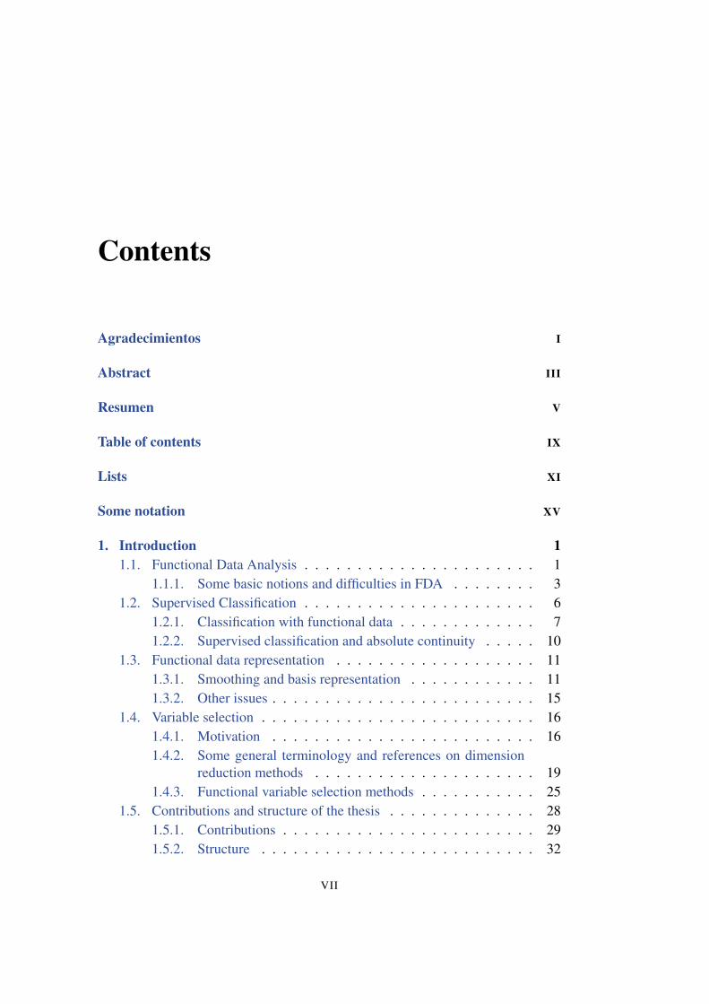
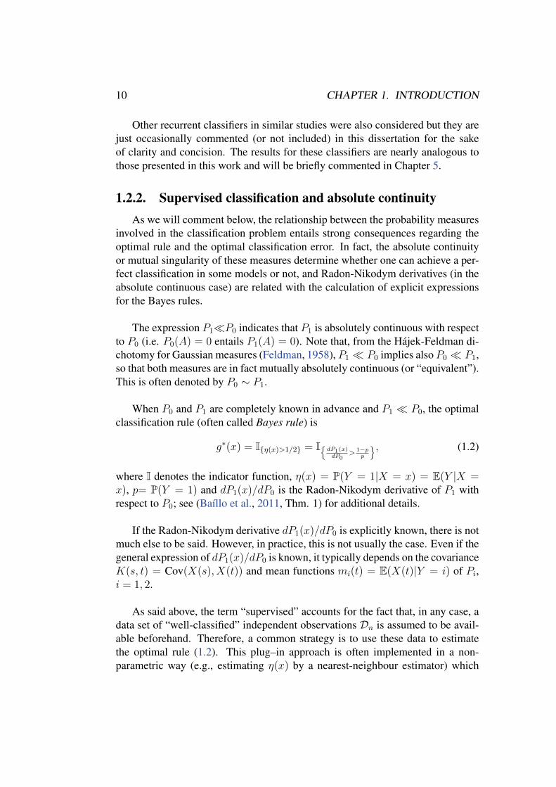
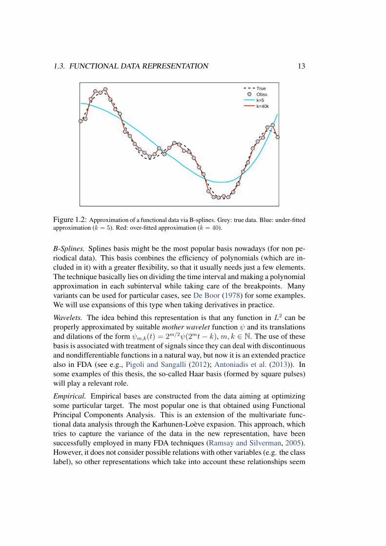
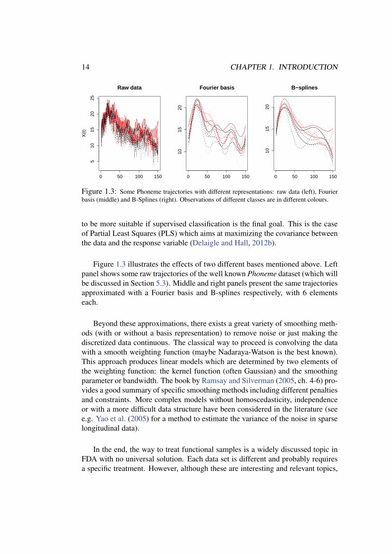
Figure 1.3: Some Phoneme trajectories with different representations: raw data (left), Fourierbasis (middle) and B-Splines (right). Observations of different classes are in different colours.
to be more suitable if supervised classification is the final goal. This is the caseof Partial Least Squares (PLS) which aims at maximizing the covariance betweenthe data and the response variable (Delaigle and Hall, 2012b).
Figure 1.3 illustrates the effects of two different bases mentioned above. Leftpanel shows some raw trajectories of the well known Phoneme dataset (which willbe discussed in Section 5.3). Middle and right panels present the same trajectoriesapproximated with a Fourier basis and B-splines respectively, with 6 elementseach.
Beyond these approximations, there exists a great variety of smoothing meth-ods (with or without a basis representation) to remove noise or just making thediscretized data continuous. The classical way to proceed is convolving the datawith a smooth weighting function (maybe Nadaraya-Watson is the best known).This approach produces linear models which are determined by two elements ofthe weighting function: the kernel function (often Gaussian) and the smoothingparameter or bandwidth. The book by Ramsay and Silverman (2005, ch. 4-6) pro-vides a good summary of specific smoothing methods including different penaltiesand constraints. More complex models without homoscedasticity, independenceor with a more difficult data structure have been considered in the literature (seee.g. Yao et al. (2005) for a method to estimate the variance of the noise in sparselongitudinal data).
In the end, the way to treat functional samples is a widely discussed topic inFDA with no universal solution. Each data set is different and probably requiresa specific treatment. However, although these are interesting and relevant topics,
1.3. FUNCTIONAL DATA REPRESENTATION 15
this thesis is not primarily concerned with this preprocessing steps but with thecomparison of different classifiers and dimension reduction techniques under thesame conditions. Then, with this criterion in mind and provided that there isno standard way to proceed, we have followed the next general practical rules(which are common in many classification and variable selection works). First,we will assume that the noise has been removed in a previous step. Second, wehave worked, when possible, with raw data. That is, we have worked preferablywith discretized data without any smoothing or basis representation. Although theelection of an adequate partition is not as trivial as it may appear at first glance(there are particular aspects of the data, such as the curvature, that have to be takeninto account) the major risk choosing a fine enough equispaced discretization gridis the increment in computing time, while the proper election of a basis or thebandwidth is much more delicate and can entail a loss of discriminant information.Moreover, it is far from clear whether smoothing would be a good practice whenclassifying functional data. The work by Carroll et al. (2013) shows that the usualsmoothing parameters (with good and even optimal performance in predictionand hypotheses testing) fail in this context, and undersmoothing is recommendedas a practical guideline. Indeed, the best results with two of the three evaluatedclassifiers are achieved with the raw data without any smoothing. Our experiencealso points to that direction, that is, smoothing is a critical issue that can entail aloss in classification accuracy. Nevertheless, in examples with extremely roughtrajectories, certain level of smoothing is frequently useful. Some examples alongboth lines will be given in this dissertation.
1.3.2. Other issuesOther common sources of problems when working with functional data are
the registration and display of the observations. Many practical concerns ariseduring the registration of the data which can frustrate even the simplest analysis.The range of registration problems includes missing or incomplete data, shift reg-istration, different scales, etc. The consideration of these issues is far beyond thescope of this work, but some reference can be found in the general bibliographyon FDA (Section 1.1). At a practical level, we will consider these problems to besolved in advance for our data.
The way of displaying functional data is more relevant for this thesis. Whatdo we mean by this? An appropriate display of functional data is not an easytask. Since we can obtain very different information looking at them in a way oranother. Usually, the standard plot of x(t) as a function of the time is less informa-tive than other possible choices. For example, important concepts in multivariatedata analysis, such as centrality or proximity, are no longer so easy to determine
16 CHAPTER 1. INTRODUCTION
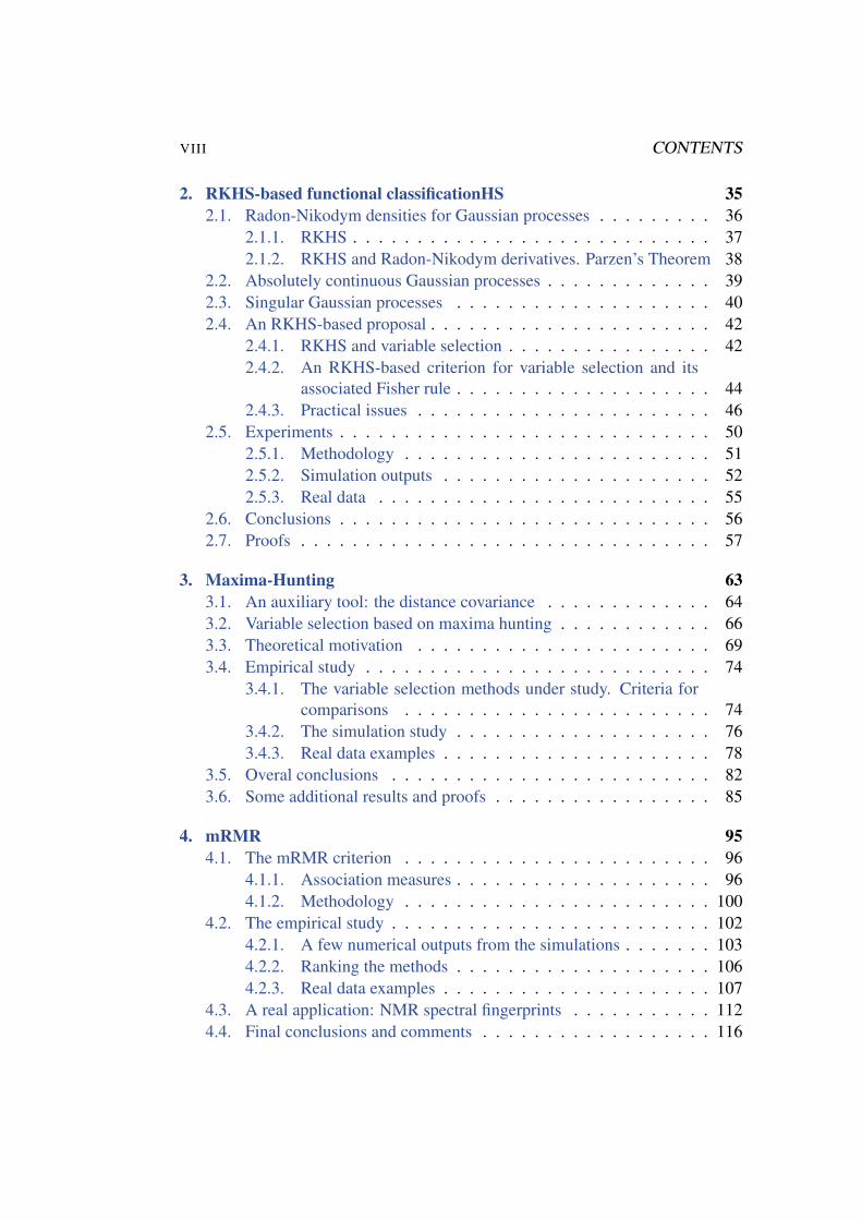
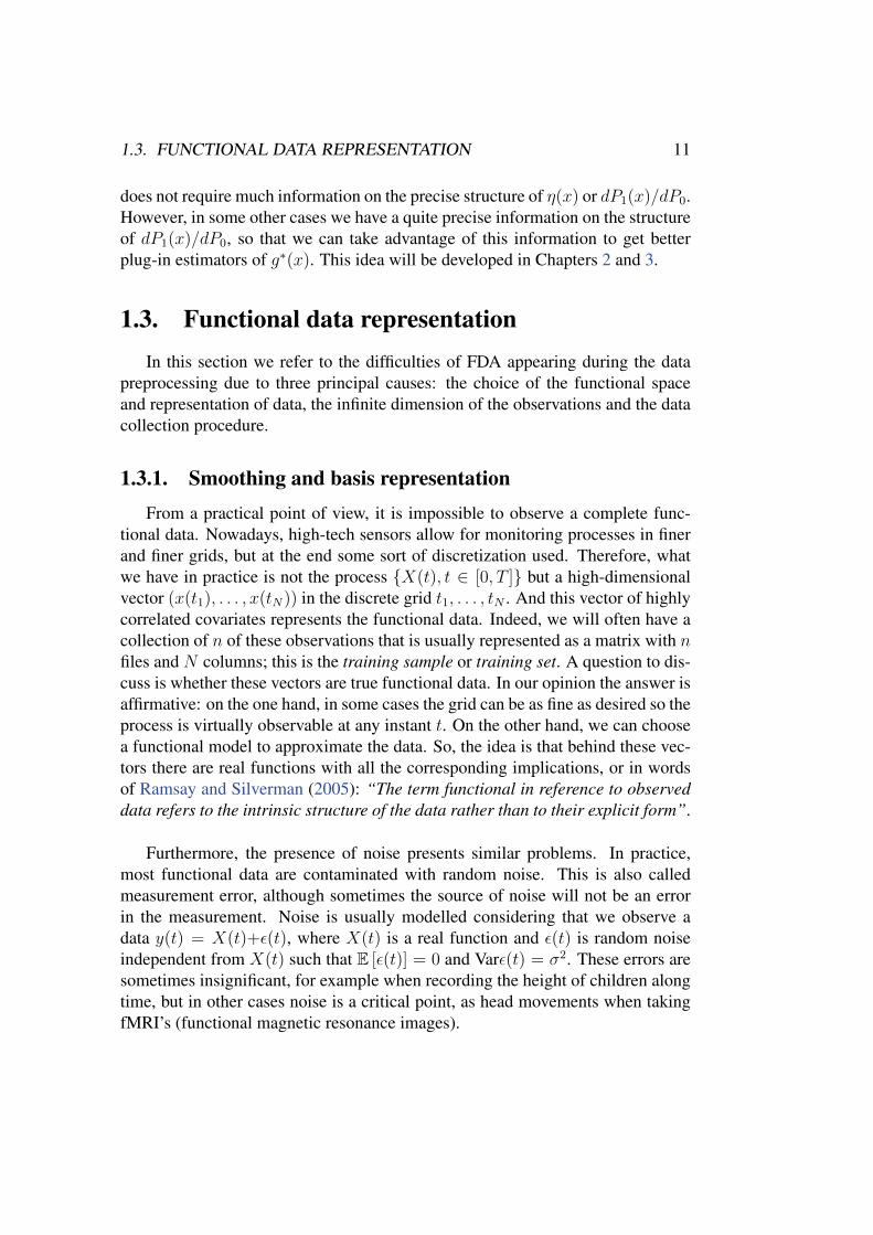
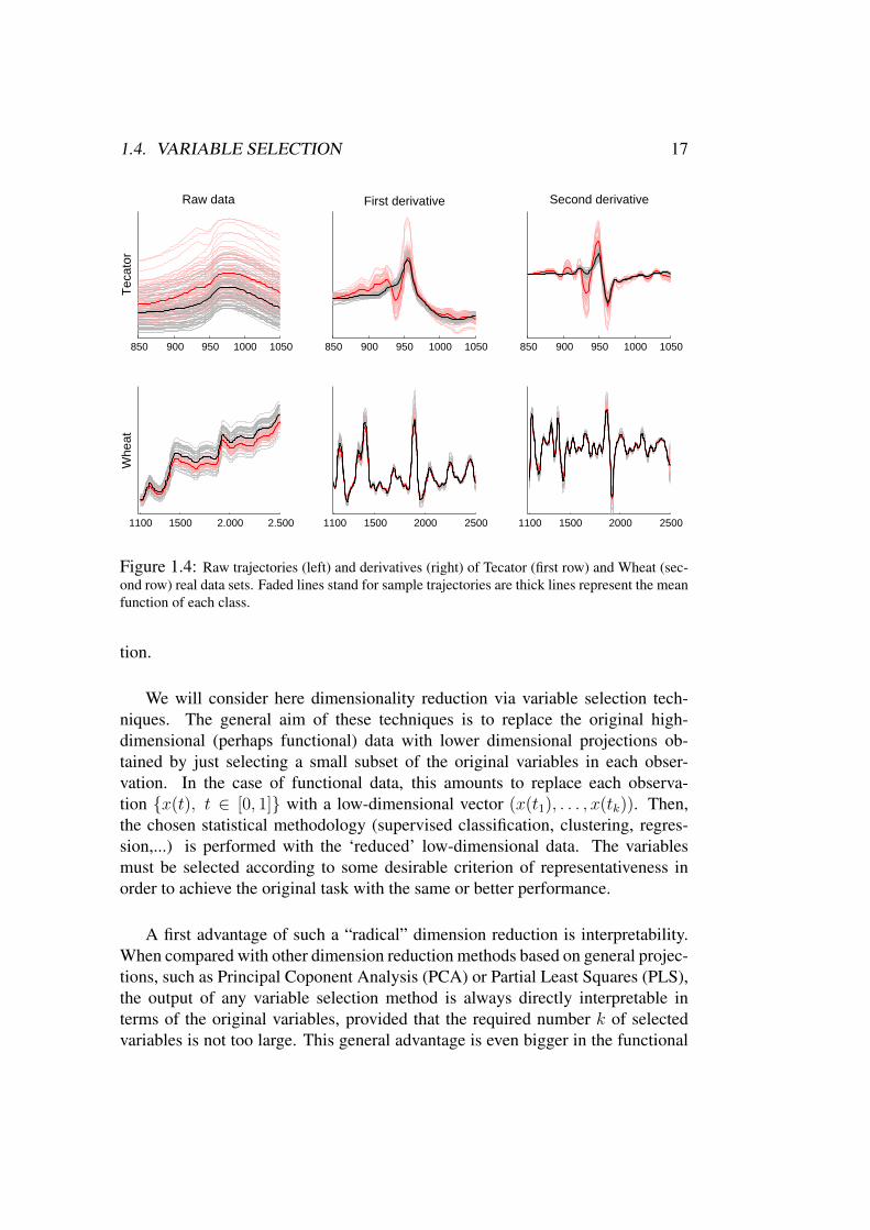
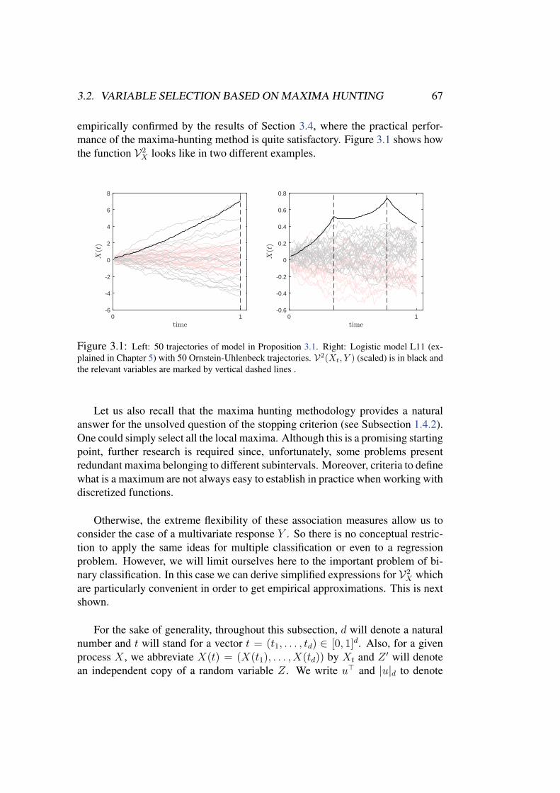
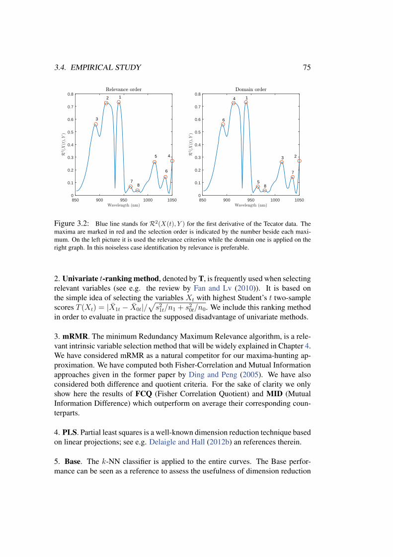
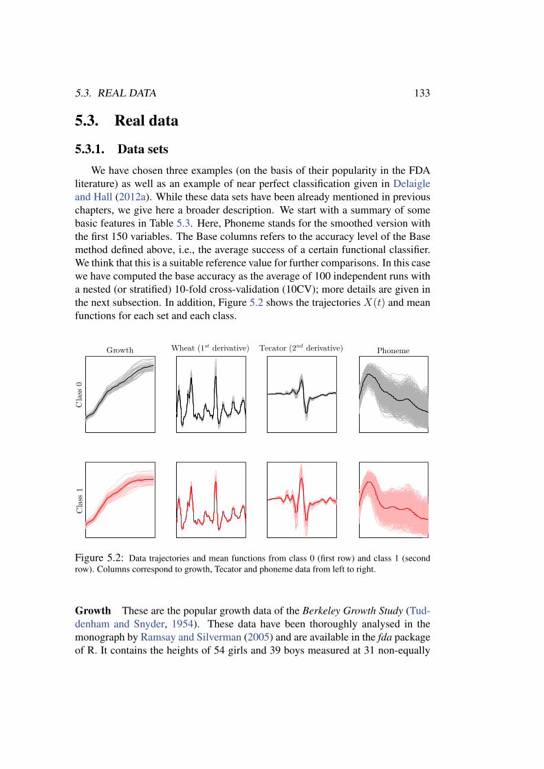
or visualize in FDA. That is a direct consequence of the functional nature com-mented in Section 1.1. Because of the non equivalence of the metrics in functionalspaces, the space in which we place the data plays a fundamental role in the infor-mation we can deduce from the data (including visual representations). Therefore,as pointed out before, a good choice of the space and an appropriate metric is a keypoint in FDA, and what might be considered as a disadvantage actually opens aworld of possibilities, which the multivariate setting lacks. Good examples of thisphenomenon are the use of different semi-metrics (see Ferraty and Vieu (2006))or the research about functional depth measures (see, e.g., Cuevas et al. (2007);Lopez-Pintado and Romo (2009)). Probably the best known examples are thoseconcerning derivatives. It is well known that, at times, derivatives are much moreinformative than the sample curves, providing new insights (many uses of thederivatives are well documented in Ramsay and Silverman (2005); Ferraty andVieu (2006)). This also happens in the supervised classification problems whenthe information provided by the derivatives turns out to be essential in some cases.A typical example which illustrates this phenomenon is given by the near infraredspectroscopy (NIR) problems. Usually, NIR data consist of very smooth and ho-mogeneous curves with small differences between the classes, so the classificationis hard. However, taking the derivatives, often reveals big differences and the clas-sification problem becomes much easier. Figure 1.4 shows this fact through tworeal NIR datasets: the classical Tecator data and a set of Wheat samples (both datasets are explained in Section 5.3). Trajectories of different classes are plotted indifferent colours. Faded lines stand for the sample trajectories while thick linesrepresent the mean function of each class. First row corresponds to Tecator andthe second one to Wheat samples. Left panel shows several trajectories of theoriginal data sets and right panels present the derivatives. The gain is quite obvi-ous and it is empirically confirmed: while raw data performance is quite modest,the derivatives achieve near perfect results (see Sections 2.5 and 3.4 for details).Finally, let us recall that in practice, taking the derivatives commonly requires aprevious smoothing step to make the data differentiable. Throughout this thesis,the derivatives have been estimated (when needed) using spline smoothing.
1.4. Variable selection
1.4.1. Motivation
The use of high-dimensional or functional data entails some important practi-cal issues. In addition to the inconveniences associated with increasing computa-tion time and storage costs, high-dimensionality introduces noise and redundancy.Thus, there is a strong case for using different techniques of dimensionality reduc-
1.4. VARIABLE SELECTION 17
850 900 950 1000 1050
Raw data
Tec
ator
850 900 950 1000 1050
First derivative
850 900 950 1000 1050
Second derivative
1100 1500 2.000 2.500
Whe
at
1100 1500 2000 2500 1100 1500 2000 2500
Figure 1.4: Raw trajectories (left) and derivatives (right) of Tecator (first row) and Wheat (sec-ond row) real data sets. Faded lines stand for sample trajectories are thick lines represent the meanfunction of each class.
tion.
We will consider here dimensionality reduction via variable selection tech-niques. The general aim of these techniques is to replace the original high-dimensional (perhaps functional) data with lower dimensional projections ob-tained by just selecting a small subset of the original variables in each obser-vation. In the case of functional data, this amounts to replace each observa-tion x(t), t ∈ [0, 1] with a low-dimensional vector (x(t1), . . . , x(tk)). Then,the chosen statistical methodology (supervised classification, clustering, regres-sion,...) is performed with the ‘reduced’ low-dimensional data. The variablesmust be selected according to some desirable criterion of representativeness inorder to achieve the original task with the same or better performance.
A first advantage of such a “radical” dimension reduction is interpretability.When compared with other dimension reduction methods based on general projec-tions, such as Principal Coponent Analysis (PCA) or Partial Least Squares (PLS),the output of any variable selection method is always directly interpretable interms of the original variables, provided that the required number k of selectedvariables is not too large. This general advantage is even bigger in the functional
18 CHAPTER 1. INTRODUCTION
setting where the interpretation of the synthetic components is still harder. In away, variable selection appears as the most natural dimension reduction proce-dure in order to keep in touch, as much as possible, with the original data. Thisis a very appreciated property in certain research areas, specially in biomedicinewhere the identification of relevant metabolites, genes, etc. for further researchis a fundamental task. For example, Dıaz-Uriarte and Alvarez de Andres (2006)point out that in microarray problems “probably a more challenging and relevantissue [than improving prediction rates] is to identify sets of genes with biologicalrelevance”. They argue that given a real data set, different classifiers often obtainanalogous results.
A second advantage is that variable selection makes sense in real problems.In most real situations, experts do not consider all the available variables sincethe relevant information is usually concentrated in some points of interest. Seefor instance Golub et al. (1999); Lindquist and McKeague (2009) among manyother examples in experimental sciences or engineering: in Golub et al. (1999)the authors note that 50 genes (among almost 7000) are enough for cancer sub-type classification. Likewise, Lindquist and McKeague (2009) point out that insome functional data regression (or classification) problems, as functional mag-netic resonance imaging or gene expression, “the influence is concentrated at sen-sitive time points”.
Third, variable selection entails classification benefits. Classifying high di-mensional and functional data involves some difficulties (curse of dimensionality,redundancy, noise, etc.) which result in a loss of classification accuracy. A suit-able variable selection method can overcome (at least partially) these problemsand lead to equivalent or even better discrimination performances with the re-duced data sets. This has been empirically shown many times in the multivariatecase, see for instance Guyon et al. (2002); Ding and Peng (2005); Dıaz-Uriarteand Alvarez de Andres (2006); Karabulut et al. (2012). This is also one of themain conclusions of the extensive experiments with functional data carried outin this thesis (see Chapters 2-5). In summary, variable selection has been empiri-cally proved to be a reliable dimension reduction methodology when the objectiveis discrimination of high dimensional and functional data.
Finally, variable selection with functional data can be also theoretically mo-tivated. Along this dissertation we will see that in several non-trivial functionalmodels, the optimal classification rule depends only on finitely many variables, sothe best we can do in these cases is finding them by means of a suitable selectionmethod.
1.4. VARIABLE SELECTION 19
1.4.2. Some general terminology and references on dimensionreduction methods
There are two main objectives that the variable selection methods should strivefor in a classification setting,
To identify relevant variables for a posterior investigation. As a matter offact, variable selection is sometimes the main target itself in many caseswhere the focus is on model simplification. Here, the most important thingis to detect all variables with significant information (in the sense of dis-crimination), no matter how big the resulting set is or how redundant theselected variables are.
To select small sets of variables that could be used for class prediction. Inthis case, we look for sets of non redundant variables that can achieve goodpredictive performances and are as small as possible.
In the present work we will focus on the second point, developing a theoreti-cal framework and providing new selection methods for that aim. Next, we willbriefly comment the principal approaches and methodologies of variable selectionto this day in order to give a context of our new contributions. Let us recall that,although only a small proportion of the existent variable selection procedures havebeen designed for functional data, the general ideas that apply in the multivariatecontext remain usually valid in the FDA setup.
There is a vast literature on variable selection published by researchers in ma-chine learning and mathematical statisticians. The approaches and the terminol-ogy used in these two communities are not always alike. Thus, in machine learn-ing language, variables are commonly called features or attributes and variableselection is often referred to as feature selection, though this term is sometimesused in a more general way to include the generation of new features. It is verycommon as well (especially in the setting of regression models) to use the terms“sparse” or “sparsity” to describe situations in which variable selection is the firstnatural aim; see e.g., Gertheiss and Tutz (2010) and Rosasco et al. (2013). It hasbeen also argued in Kneip and Sarda (2011) that the standard sparsity models aresometimes too restrictive, so that it is advisable to combine them with other di-mension reduction techniques. The “relevant” variables in a functional model aresometimes called “impact points” (McKeague and Sen, 2010) or “most predictivedesign points” (Ferraty et al., 2010). Also, the term “choice of components” hasbeen used by Delaigle et al. (2012) as a synonym of variable selection.
20 CHAPTER 1. INTRODUCTION
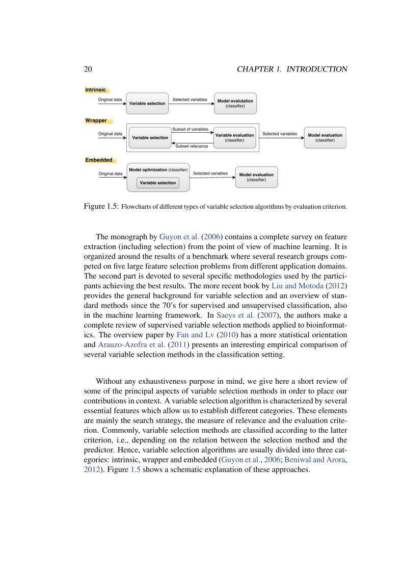
Figure 1.5: Flowcharts of different types of variable selection algorithms by evaluation criterion.
The monograph by Guyon et al. (2006) contains a complete survey on featureextraction (including selection) from the point of view of machine learning. It isorganized around the results of a benchmark where several research groups com-peted on five large feature selection problems from different application domains.The second part is devoted to several specific methodologies used by the partici-pants achieving the best results. The more recent book by Liu and Motoda (2012)provides the general background for variable selection and an overview of stan-dard methods since the 70’s for supervised and unsupervised classification, alsoin the machine learning framework. In Saeys et al. (2007), the authors make acomplete review of supervised variable selection methods applied to bioinformat-ics. The overview paper by Fan and Lv (2010) has a more statistical orientationand Arauzo-Azofra et al. (2011) presents an interesting empirical comparison ofseveral variable selection methods in the classification setting.
Without any exhaustiveness purpose in mind, we give here a short review ofsome of the principal aspects of variable selection methods in order to place ourcontributions in context. A variable selection algorithm is characterized by severalessential features which allow us to establish different categories. These elementsare mainly the search strategy, the measure of relevance and the evaluation crite-rion. Commonly, variable selection methods are classified according to the lattercriterion, i.e., depending on the relation between the selection method and thepredictor. Hence, variable selection algorithms are usually divided into three cat-egories: intrinsic, wrapper and embedded (Guyon et al., 2006; Beniwal and Arora,2012). Figure 1.5 shows a schematic explanation of these approaches.
1.4. VARIABLE SELECTION 21
Intrinsic The methods we have called “intrinsic” are often denoted as “filtermethods” in machine learning literature. In intuitive terms, the intrinsic methodsaim at extracting (via variable selection) the information present in the data, in-dependently of the use given to such data. Typically, variables are sorted by anyrelevance measure and those with lower score are removed. Thus, this approachis usually computationally simple, efficient and fast, so intrinsic methods read-ily scale high-dimensional problems. Since they are independent of the predictorthey are more generalizable, that is, different classifiers can be evaluated with thesame selected subset of variables. Also, the overfitting risk is smaller than in theother paradigms. However, this independence could be the main drawback of in-trinsic techniques since they ignore any possible interaction with the classificationrule. Besides the general references mentioned above, some intrinsic methods arereviewed in Lazar et al. (2012) for gene selection problems. A relevant exampleof intrinsic algorithms is the so called mRMR (minimum Redundancy MaximumRelevance) method, proposed by Ding and Peng (2005). See Chapter 4 for furtherdetails on this method along with a modified version and new applications.
Wrapper These are popular techniques since the publication of the paper byKohavi and John (1997). Wrapper methods receive this name because the selec-tion procedure “wraps” the predictor. The classification rule is used as a black boxto assign scores to the different subsets of variables according to their discriminantpower. In other words, the quality of a set of variables is directly measured by theperformance of a predictor that only uses these variables. The algorithm carriesout a double search, the first one considers all possible subsets of variables andthen the classifier is estimated from each set. Hence, wrapper methods are compu-tationally expensive and slow. In addition, they are not generalizable: the resultingselection is valid only for the considered classifier so, if different predictors mustbe studied, the whole process must be repeated for each predictor. The principaladvantages of wrapper methods are that they take into account relations amongvariables in a natural way, and the connection with the predictor, which leads tobetter classification accuracy. However, this connection also entails a higher riskof overfitting than that of intrinsic methodologies. Many wrapper methods havebeen developed because of their good performance. SVM is one of the classifiersmore utilized for these techniques methodology (Maldonado and Weber, 2009).
Embedded This third category is sometimes omitted or included as a specialcase of wrapper methods, but it represents a different approach. In this setup,variable selection and model estimation are performed simultaneously throughthe optimization of a target function. Then, embedded methods have closer con-nections between the selected variables and the predictor, so in this sense they
22 CHAPTER 1. INTRODUCTION
present same advantages and disadvantages as wrapper methods, but accentuated.Most interactions are taken into account, but embedded methods are totally de-pendent on the chosen model. However, mixing the selection process and themodel estimation is usually less computationally expensive than the wrapper ap-proach and can lead to a better use of the available data since it does not requireto split the training sample for validation (Saeys et al., 2007). Maybe the mostpopular embedded methods are LASSO (Tibshirani, 1996) and variable selectionvia Random-Forest (Dıaz-Uriarte and Alvarez de Andres, 2006); see Scornet et al.(2015) for a general reference on random-forest with mathematical theory. Manyother methodologies have been adapted to embedded variable selection, for exam-ple, SVM (Guyon et al., 2002).
Hybrid Finally, in the latest years there have appeared hybrid or two-stepsmethods which try to take advantage of the strengths of intrinsic and wrapper ap-proaches avoiding their weaknesses. The general idea is to combine intrinsic andwrapper methods in two-steps algorithms. First, an intrinsic procedure is used inorder to filter the informative variables by removing useless (and sometimes re-dundant) variables, and then a wrapper algorithm is applied to this reduced set;see for instance, Hua et al. (2009); Hsu et al. (2011).
We are especially interested in the “intrinsic” approaches to variable selection,in the sense that the final output should depend only on the data, not on any as-sumption on the underlying model (although the result should be interpretable interms of the model).
Another fundamental issue in variable selection is how to decide whether avariable (or a set of variables) is relevant or not. Remember that our aim is toremove redundant or irrelevant variables in order to get the best classification per-formance with the smallest possible number of variables. There is not an universaldefinition for the relevance or the importance of a variable since this depends oneach particular problem. However, some attempts to formalize these conceptshave been done, see e.g. Yu and Liu (2004); Guyon et al. (2006). Roughly speak-ing, a group of variables is relevant in the classification setting if they have a highdiscriminant power, and irrelevant otherwise. Algorithms use different associationmeasures I(·, ·) to estimate the amount of discriminant information of a variableX in terms of its relation with the class Y . Thus, the usual relevance indicatoris I(X, Y ). Standard correlation based measures were the first choice for I andthey are still commonly used as relevance indices (Hall, 1999). Other optionslike the gain ratio (Quinlan, 1996), the Gini index (used by Breiman (2001) inrandom forest) or Relief-F (an extension of Relief to deal with sets of continu-
1.4. VARIABLE SELECTION 23
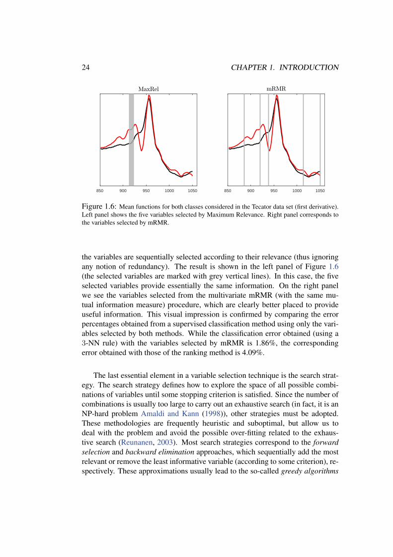
ous variables by Robnik-Sikonja and Kononenko (2003) ) are also popular amongpractitioners. A good summary of standard criteria of relevance can be found inGuyon et al. (2006, Chapter 3). Nowadays, the preferred relevance indices mightbe those based on distance between distributions. Two examples of this approachare considered in this thesis. The popular mutual information measure, which hasled to a wide range of procedures [see Vergara and Estevez (2014) for a compre-hensive survey], is commented in Chapter 4. Besides, we propose the use of therecent distance correlation measure (Szekely et al., 2007) in two different waysin Chapters 3 and 4.
Depending on the use of the relevance measure, variable selection methodscan be univariate or multivariate (in machine learning terminology). The for-mer are usually called ranking methods since the variables are simply rankedby the relevance score I(X, Y ). In this setting, variables are considered sepa-rately, regardless of the classifier and ignoring any kind of dependence amongthem. These methods have been extensively used due to their simplicity, speedand good performance in a variety of problems (Saeys et al., 2007; Fan and Lv,2010). However, ranking methods do not take into account relationships amongvariables. In particular, they do not remove the redundancy among them, whichis a critical point when dealing with functional data. On the other hand, the term“multivariate” stands for those methods which consider, in some sense, variabledependencies to overcome the redundancy problem. Also, some multivariate al-gorithms can take advantage of the positive interactions between variables (it iswell known that some variables can be irrelevant individually but very informa-tive when they work together). Some examples of this multivariate strategy are themethods based on mRMR (Ding and Peng, 2005; Ponsa and Lopez, 2007), whichselect iteratively the variables that maximize the relevance and minimize the re-dundancy at the same time, or the Correlation-based Feature Selection (CFS) byHall (1999), that measures the correlation between pairs of variables. Anotherpopular representatives of this approach are the Relief method and its versions formulticlass and regression problems, ReliefF and RRelief respectively (Robnik-Sikonja and Kononenko, 2003; Guyon et al., 2006). The underlying idea in thesemethods is to take advantage of the nearest neighbours methodology to choose thebest subset of variables.
The following example shows that the multivariate approach may be substan-tially better than the univariate one in the functional context. It refers to the well-known Tecator data set (a benchmark example very popular in the literature onfunctional data; see Section 5.3 for details). To be more specific, we use the firstderivative of the curves in the Tecator data set, which is divided into two classes.We first use a simple ‘ranking procedure’ based on the mutual information, where
24 CHAPTER 1. INTRODUCTION
850 900 950 1000 1050
MaxRel
850 900 950 1000 1050
mRMR
Figure 1.6: Mean functions for both classes considered in the Tecator data set (first derivative).Left panel shows the five variables selected by Maximum Relevance. Right panel corresponds tothe variables selected by mRMR.
the variables are sequentially selected according to their relevance (thus ignoringany notion of redundancy). The result is shown in the left panel of Figure 1.6(the selected variables are marked with grey vertical lines). In this case, the fiveselected variables provide essentially the same information. On the right panelwe see the variables selected from the multivariate mRMR (with the same mu-tual information measure) procedure, which are clearly better placed to provideuseful information. This visual impression is confirmed by comparing the errorpercentages obtained from a supervised classification method using only the vari-ables selected by both methods. While the classification error obtained (using a3-NN rule) with the variables selected by mRMR is 1.86%, the correspondingerror obtained with those of the ranking method is 4.09%.
The last essential element in a variable selection technique is the search strat-egy. The search strategy defines how to explore the space of all possible combi-nations of variables until some stopping criterion is satisfied. Since the number ofcombinations is usually too large to carry out an exhaustive search (in fact, it is anNP-hard problem Amaldi and Kann (1998)), other strategies must be adopted.These methodologies are frequently heuristic and suboptimal, but allow us todeal with the problem and avoid the possible over-fitting related to the exhaus-tive search (Reunanen, 2003). Most search strategies correspond to the forwardselection and backward elimination approaches, which sequentially add the mostrelevant or remove the least informative variable (according to some criterion), re-spectively. These approximations usually lead to the so-called greedy algorithms
1.4. VARIABLE SELECTION 25
which approximates the global optimum by a local one at each step and generatenested subsets of variables. The sequential forward search (SFS) and the analo-gous backward procedure (SBS) are two examples of this approach (Kittler, 1978).Some interesting alternatives are random searches where the space of variables isexplored in an “arbitrary” way. Some relevant examples of this technique aregenetic algorithms (Leardi et al., 1992) and simulated annealing (Brusco, 2014).See, e.g. Guyon et al. (2006); Liu and Motoda (2012) for further details and strate-gies. Besides, mixture approaches combining different strategies have been alsoconsidered, for example the “plus-l-take-away-r” methodology which combinesforward and backward searches; see Vergara and Estevez (2014) for a survey fo-cused on intrinsic methods.
The question of when to stop the search has not an unique answer so far. Thisis a sensitive issue, since too many or too less variables can affect heavily theresults. There are numerous alternatives in the literature. Many times (speciallyin applied sciences) the number of variables is fixed arbitrarily based on cost,time or other reasons. For example, Golub et al. (1999) and Nguyen and Rocke(2002) uses the best 50 genes for their analysis. Other criteria can be a maximumnumber of loops (specially in random algorithms), a score threshold, to reachcertain complexity level, etc.; see, e.g., Liu and Motoda (2012, Chapter 3) forfurther details and references. In this thesis we will use a standard validationstep (via either cross-validation or using a validation sample) to set the number ofvariables (Guyon et al., 2006). Note however that we are not primarily concernedwith the choice of the best number of variables but with establishing standardconditions in order to fairly compare the methods under study.
Many other aspects of variable selection methods could be considered, butthey are beyond the scope of this work. We refer to the books and reviews citedin this section for further details and references.
1.4.3. Functional variable selection methodsIn the functional setting, several relevant dimension reduction techniques are
based upon the use of general finite dimensional projections. This is the case offunctional principal component analysis (FPCA), see Li et al. (2013), although theso-called partial least squares (PLS) methodology is in general preferable when aresponse variable is involved; see Delaigle and Hall (2012b) for a recent referenceon functional PLS. Functional PCA is adapted to sparse longitudinal data in Yaoet al. (2005). Other common dimension reduction methods in the functional set-ting include sliced inverse regression (Hsing and Ren, 2009; Jiang and Liu, 2014)and additive models (Zhang et al., 2013). Also, the methods based on random pro-
26 CHAPTER 1. INTRODUCTION
jections could offer an interesting alternative. See, e.g., Cuevas (2014) for a shortoverview of dimension-reduction techniques together with additional references.
Nevertheless, we are concerned here with a different, more radical, approachto dimension reduction given by variable selection methods. As mentioned before,the aim of variable selection when applied to functional data is to replace everyinfinite dimensional observation x(t), t ∈ [0, 1] with a finite dimensional vec-tor (x(t1), . . . , x(tk)). However, the reduction procedure must take into accountthe special characteristics of functional data, specially the high redundancy be-tween close variables. Hence, the selection of the “variables” t1, . . . , tk should bea consequence of a trade-off between two mutually conflicting goals: representa-tiveness and parsimony. In other words, we want to retain as much information aspossible (thus selecting relevant variables) employing a small number of variables(thus avoiding redundancy).
Despite the huge amount of literature about variable selection for multivariatedata, much less references are available when dealing with functional data, andmost of them and centred in the linear regression framework. Today the most pop-ular variable selection method among statisticians is perhaps the so-called LASSOprocedure, proposed by Tibshirani (1996), as well as the Dantzig selector, a mod-ification of LASSO, proposed by Candes and Tao (2007). These methods havea nice heuristic motivation and good theoretical properties; moreover, as shownby Bickel et al. (2009), they are asymptotically equivalent. Their application tothe functional data setting has been analyzed by Kneip and Sarda (2011). Also,Zhou et al. (2013) adapt SCAD ideas for zero-coefficients to the functional set-ting. Other examples which also use L1 regularizations in this context are Lee andPark (2012); Gertheiss et al. (2013); Zhao et al. (2014). The Partial Linear Regres-sion (PLR) model is extended to functional covariates by Aneiros-Perez and Vieu(2006), and by Ferraty and Romain (2011, Chapter 3), where variable selectionand estimation of coefficients are carried out simultaneously. Besides, let us alsomention, with no attempt to be exhaustive, that the recent literature in functionalvariable selection includes a study of consistency in this setup (Comminges andDalalyan, 2012). Also, James et al. (2009) gives an “interpretable” variable selec-tion method which uses the derivatives of the function of coefficients jointly with agood and concise review of variable selection methods for high-dimensional linearregression. A wrapper procedure is proposed in the same linear regression frame-work by Ferraty et al. (2010). The “most predictive design points” are chosen tominimize the cross-validation error of a local linear regression method. The recentpaper by Aneiros and Vieu (2014) introduces a two-stages procedure which usesthe continuity of the functional predictors in order to get a better performance.
1.4. VARIABLE SELECTION 27
The application of these methods has been mostly developed for models. Infact, their formal implementation relies essentially on the assumed model. In thepresent work our approach to variable selection is slightly different, in the sensethat we look for “intrinsic” methods based on the data and not relying on any as-sumption on a particular model (e.g. linear regression). Moreover, throughout thisthesis we will consider variable selection in the setting of functional supervisedclassification (the extension to more general regression problems is also possiblewith some obvious changes). Surprisingly, variable selection for functional dataclassification is rarely addressed in both machine learning and statistical litera-ture. Most of the existing references are focused on the classification of functionalmagnetic resonance images (Grosenick et al., 2008; Ryali et al., 2010) and nearinfrared spectra (Xiaobo et al., 2010). But in most cases curves are just treatedas multivariate data for which the usual methods apply, and sometimes they areonly used to extract some new (synthetic) variables which are the real objectsin the variable selection phase. This happens, for example, in Gomez-Verdejoet al. (2009) which initially analyse the same problem as we do: variable selectionfor functional data classification. However, these authors propose to transformthe functions into vectors of different artificial components extracted from thecurves. Then, a new multivariate feature selection method is applied to these newhigh-dimensional observations. From a entirely functional point of view, Delaigleet al. (2012) provide a variable selection method for classification and cluster-ing using the same approach of minimizing the cross-validation error as Ferratyet al. (2010). In both cases several heuristic adjustments are proposed in orderto lighten the computational load typical of wrapper approaches. A new type oflogistic regression model for binary classification of functional data is proposedby Lindquist and McKeague (2009), who consider Brownian-like predictors (e.g.fMRI and gene expression). A similar approach is followed in McKeague andSen (2010) for fractional Brownian trajectories. Matsui (2014) introduces a L1-penalized logistic model for multiclass classification.
Finally, some similar approaches should be mentioned even though they arenot purely variable selection methods. For example, one can think on selectingintervals instead of points. In this way, the paper by Li and Yu (2008) provides aclassification method for functional data based on “short curve segments”. Tianand James (2013) propose the selection of some basic “interpretable” functions torepresent the curves (a sort of wavelet basis) before classification. These elementsare chosen by minimizing the misclassification error through a stochastic search.An interpretable SVM-based classifier which allows us to consider “different lev-els of interpretability”, is provided by Carrizosa et al. (2011). Finally. a differentapproach is followed by Fraiman et al. (2015), where the selection is carried outafter a “satisfactory” analysis of the data (regression, classification or principal
28 CHAPTER 1. INTRODUCTION
components). The goal is being able to “replicate” the result of the previous sat-isfactory analysis with a reduced dataset. This is obtained via several functionswhich capture relevant features of the original data (pointwise evaluation, localaverages, moments, etc.). The selection is performed on a number of these specialfunctions with a mixed search strategy (exhaustive and stochastic).
Our purpose in this thesis is to contribute to the study of the variable selec-tion problem in a functional framework when classification is the final goal. Onthe one hand, a full theoretical motivation is given for these techniques, and onthe other hand some new methodologies feasible for functional data are proposed.In particular, we present three intrinsic procedures for variable selection, i.e. notrelying on any particular assumption on the dependence model. These methodshave a sound functional motivation, and all of them adopt procedures to deal withthe strong redundancy of the functional data sets. The use of the forward searchstrategy contributes to an easy comprehension and implementation, which is usu-ally fast. All these methods are intrinsic, that is, they are (in principle) suitablefor general problems and different classifiers. Despite these common features, thenew proposed methods correspond to three different ideas. The first method, seeBerrendero et al. (2015a), is called Reproducing Kernel Variable Selection (RK-VS) and is based on the maximization of the Mahalanobis distance between themultivariate means corresponding to the selected variables of the two classes. Itcan be justified from an RKHS point of view and is explained in Chapter 2. Sec-ond, the Maxima-Hunting procedure (MH), see Berrendero et al. (2015c), reliesonly on the direct use of the distance correlation measure by Szekely et al. (2007).This is fully described in Chapter 3. The last method, presented in Chapter 4,represents a modification of the mRMR algorithm, based on an idea we believespecially suitable for functional data. So we adapt this idea here, in combinationwith the distance correlation, for its use in the functional case (Berrendero et al.,2015b).
1.5. Contributions and structure of the thesisThis is concerned with the problem of supervised binary classification with
functional data. We consider the functional data as trajectories drawn from astochastic process. As a consequence, we will try to motivate our results andproposals in terms of this underlying stochastic process. This is somewhat incontrast with the mainstream research line in FDA, mostly centred in algorithmicaspects and real data analysis.
In short, the original contributions in this work are the following:
1.5. CONTRIBUTIONS AND STRUCTURE OF THE THESIS 29
a) General mathematical theory for the functional classification problem. It isclosely related with the reproducing kernel Hilbert space (RKHS) associ-ated with the covariance operator of the processes.
a1) We provide some explicit expressions for the Bayes (optimal) rule andits corresponding error for the problem of classifying between abso-lutely continuous Gaussian processes.
a2) A complete mathematical treatement is given for the case of the clas-sification between to mutually singular processes, which correspondsto the so-called near perfect classification phenomenon.
b) Functional variable selection.
b1) A general theoretical motivation (expressed in terms of a sparsity as-sumption) is given for the problems of functional variable selection.
b2) We propose three new variable selection methods: RK-VS (an RKHS-based selector), MH (a “maxima-hunting” method) and mRMR-RD (amodified version of the popular mRMR procedure).
c) Numerical experiments. We provide the largest simulation study on func-tional variable selection we are aware of. Some popular data examples arealso analysed together with a further real example with metabolic data.
The papers Berrendero et al. (2015b) and Berrendero et al. (2015c) correspondrespectively to the mRMR-RD and MH proposals mentioned above. The contribu-tions of point a) and the RK-VS method are essentially included in the manuscriptBerrendero et al. (2015a). A more detailed explanation of this outline is given inthe next subsections.
1.5.1. ContributionsThe contributions of this thesis are threefold. Firstly, the supervised classifica-
tion of functional data is tackled in a relatively unexplored point of view. Problemsare characterized in terms of the absolute continuity or mutual singularity of theunderlying probability measures, which entails some intriguing consequences inthe functional classification setting. In the absolutely continuous case P1 P0,some classical results concerning calculation of Radon-Nikodym derivatives forprobability measures in function spaces are used in order to obtain and interpretexplicit expressions for the optimal classifier in some binary functional discrimi-nation problems of practical interest. This approach leads to a new class of plug-inclassifiers. In some relevant cases the optimal rules turn out to depend on a finite
30 CHAPTER 1. INTRODUCTION
number of variables, so that the use of variable selection methods is especially ap-propriate. These results provide a theoretical basis for the techniques of variableselection in functional classification models. Usually these methods are consid-ered in the literature from an exclusively algorithmic or computational point ofview. Therefore, it is of some interest to motivate them in “population terms”,by identifying some specific models where these techniques have a clear mean-ing. The present dissertation can be seen as a partial contribution to this kind ofmotivations.
We also consider the mutually singular case P0⊥P1, i.e., when there exist aBorel set A such that P0(A) = 1 and P1(A) = 0. Note that this mutually singu-lar (or “orthogonal”) case is rarely found in the finite-dimensional classificationsetting, except in a few trivial or artificial cases. However, in the functional frame-work the singular case is an important general situation. We show that this mutualsingularity notion is behind the near perfect classification phenomenon describedin Delaigle and Hall (2012a). The point is to look at this phenomenon from theslightly different (coordinate free) RKHS perspective. We also show that an ap-proximately optimal (“near perfect”) classification rule to discriminate betweenP0 and P1 when P1 ⊥ P0, can be obtained in terms of the optimal rules corre-sponding to a sequence of problems (P n
0 , Pn1 ) with P n
1 P n0 .
Second, we offer three new intrinsic methods for variable selection precedingfunctional discrimination. In the first place we propose a flexible RKHS-basedvariable selection mechanism which arises in a natural way from the theoreticalframework. Unlike other popular variable selection methods in classification, thisnew proposal allows the user to incorporate, in a flexible way, different amountsof information (or assumptions) on the underlying model. We also provide a con-sistent closely related linear classifier. An empirical study shows that both thevariable selection method and the associated classifier, perform very well and areclearly competitive with respect to existing competing alternatives. We also argue,as an important additional advantage, the simplicity and ease of interpretation ofthe RKHS-based procedures.
The second proposed method is based on a direct use of the distance covari-ance measure V2, or alternatively the distance correlation measure R2, proposedby Szekely et al. (2007): we just propose to select the variables indices t1, . . . , tkin the functional data X(t), t ∈ [0, 1], which correspond to local maxima of thesedistance covariance/correlation functions between X(t) and the response variableY . So one always know the exact meaning of the selected variables: they arejust those locally maximizing the dependence with the response variable. We willmotivate this “maxima hunting” (MH) idea via some theoretical models for which
1.5. CONTRIBUTIONS AND STRUCTURE OF THE THESIS 31
the optimal (Bayes) rule turns out to be explicitly known. The practical imple-mentation of the method, for a given data set, arises as a result of the estimationof V2(Xt, Y ) or R2(Xt, Y ). This is backed by a consistency result and we alsoprovide some new alternative versions of the distance covariance measure when Yis a binary variable. An exhaustive empirical study shows the good performanceof this new approach when compared with other competitors.
The third proposed selection method is a modified version of the mRMR al-gorithm by Ding and Peng (2005), in which the association between the variablesis calculated by means of different measures. We consider several versions of themRMR and compare them by an extensive empirical study. Two of these versionsare new: they are based on the distance covariance and distance correlation as-sociation measures commented above. Our results suggest that the new versionbased on the distance correlation measure represents a clear improvement of themRMR methodology in the functional framework. This method has been alsosuccessfully applied in a real problem for discriminating mice with different sexand diet from their NMR spectral fingerprints (Barba et al., 2015).
Additionally to these new proposals and results, the third major goal of thiswork is to provide an extensive and replicable empirical study aimed at assess-ing the performance (in the setting of binary functional classification) of severalintrinsic variable selection methods. In this empirical study (which includes alarge number of simulations and a few real data examples) the variable selectionmethods are viewed as particular instances of the dimension reduction method-ology. Thus we have included in the comparisons different selection techniquesand the PLS method as a reference, since it is, by now, the most usual procedurefor dimension reduction in functional data analysis before discrimination. In allcases the classifiers under study are chosen as a sort of all-purposes benchmarkmethods. Of course other functional classifiers could be considered but since thestudy is centred on intrinsic variable selection methods, the interpretability of theresults would be greatly complicated if new “variables” (in this case, differentclassifiers or tuning parameters) were introduced. To our knowledge, this is thelargest empirical study on variable selection so far.
Finally, as a consequence of all the revision work we have carried out, this the-sis presents a general overview of variable selection in a functional classificationframework. Also some empirical result and details about some well known realdata sets have been summarized.
32 CHAPTER 1. INTRODUCTION
1.5.2. Structure
This thesis is organized in six chapters and one appendix. After this intro-ductory chapter, which states the problem and reviews the general literature aboutthe related topics, the next three chapters contain the main contributions of thiswork. Roughly speaking, each chapter corresponds to a different approach to thevariable selection problem when classifying functional data.
In Chapter 2 we study the supervised classification of functional data from thenovel point of view based on the RKHS theory. Some background on this theoryis given in Section 2.1. As a consequence of this approach, we provide theoreticalmotivation for variable selection when classifying Gaussian processes, as well asshed some light on some phenomenons around functional classification. First,the explicit expressions of the optimal rules for the case of equivalent processes(Thm. 2.2) can be found in Section 2.2. Second, the mutual singular settingis considered in the next section: this orthogonality is shown to be behind thenear perfect classification phenomenon(Thm. 2.4) and an approximately optimalclassification rule for this case is derived in Theorem 2.5. In the third place, theRKHS-based variable selection method and the related classifier are proposed inSection 2.4. A consistency result for RKHS-based classifier is given in Thm. 2.6.The performance of these new techniques is assessed in Section 2.5. Section 2.7contains all the proofs of this chapter.
The maxima hunting method is presented in Chapter 3. In Section 3.1 weprovide a survey of the main ideas and results concerning the distance covarianceand distance correlation measures. Some useful simplified versions for V2 areobtained in Theorem 3.1, for the particular case where Y is a binary variable. Themaxima hunting method for variable selection is described in Section 3.2. Resultsof consistent estimation (Thm. 3.2, Lemma 3.1) for the maxima of V2 is alsoproved in that section. In Section 3.3 we give several models (identified in termsof the conditional distributions X(t)|Y = j) for which the optimal classificationrule depends only on a finite number of variables. We also show that in some ofthese models the variables to be selected coincide with the maxima of V2. Finally,some empirical results with both simulation and real data examples are given inSection 3.4 together with a brief discussion. All the proofs of this chapter are inSection 3.6.
Chapter 4 corresponds to the new version of the minimum Redundancy Max-imum Relevance (mRMR) algorithm. Section 4.1 contains a summary and someremarks about the mRMR methodology. The different association measures un-der study (which are used to define the different versions of the mRMR method)
1.5. CONTRIBUTIONS AND STRUCTURE OF THE THESIS 33
are explained in Subsection 4.1.1. The empirical study, consisting of simulationexperiments and some representative real data sets, is explained in Section 4.2.Finally, the real application is described in section 4.3 and some conclusions aregiven.
Extensive simulation studies, comparing our variable selection methods withother dimension reduction procedures (as well as with the “baseline option” of do-ing no variable selection at all) have been tackled for all the new methods. Someparticular results are given in the corresponding chapters but the general method-ology, the considered models and other empirical issues are detailed in Chapter5 aiming at not duplicating information and making the study replicable by inter-ested researchers. The methods under study and their implementation details arecommented in Section 5.1. The simulation study is fully explained in Section 5.2,including the description of the models and the followed methodology. Four realdata sets are discussed in Section 5.3 as well as the methodological differences.This Chapter also includes some additional outputs of our new proposals.
Finally, Chapter 6 contains some general conclusions that can be extractedfrom this work together with some potential lines of future research.
The full list of simulation models is in Appendix A.
Chapter 2
RKHS-based functionalclassification
Functional data classification has been always studied in the usual spaces offunctions (essentially L2[a, b], C[a, b] and some semi-normed spaces). In thischapter we propose to tackle the problem from the Reproducing Kernel HilbertSpaces (RKHS) associated with the covariance function of the underlying processwhich generates the data. RKHS theory was first applied by Parzen (1961) insignal detection problems, where no samples were involved and the approach isquite different to that we will follow here. However, this and other works (Parzen,1962; Kailath, 1971; Segall and Kailath, 1975) developed a collection of toolswhich are also very useful in our functional discrimination problem. But aboveall, the RKHS view opens the door to a new manner of dealing with stochasticprocesses in different spaces that are intrinsically connected with the processesand the classification problem. In words of Parzen (1961):“It turns out, in myopinion, that reproducing kernel Hilbert spaces are the natural setting in which tosolve problems of statistical inference on time series”. Note that Parzen uses herethe expression “time series” as a synonym of stochastic processes, which is ratherunusual in the modern statistical terminology.
This chapter begins with a brief review of some relevant background about theRKHS theory related with the classification problem. Some important results forthis chapter about characterizations of the probability measures (equivalence ormutually singularity) and expressions of the Radon-Nikodym derivatives (in theabsolutely continuous case) for Gaussian processes are given in Subsection 2.1.2.The absolutely continuous case is considered in Section 2.2, where the previousresults are used to derive explicit expressions of the optimal classification rule(Thm. 2.2) through the Equation (1.2). Section 2.3 is devoted to mutually sin-
35
36 CHAPTER 2. RKHS
gular measures. Here, the near perfect classification result by Delaigle and Hall(2012a) is explained in terms of the orthogonality of the distributions (Thm. 2.4)and Theorem 2.5 provides a method to approximate the Bayes rule in the singu-lar framework by means of a sequence of approximating (absolutely continuous)problems. In Section 2.4 the RKHS approach is used in order to define a theo-retical framework for variable selection under a reasonable sparsity assumption.This fact is exploited by constructing a flexible RKHS-based variable selectionmethod and an associated classification rule in Subsection 2.4.2. These methodsare backed by a consistency result (Thm. 2.6) and the good results of the experi-ments of Section 2.5. The possibility of adding extra information along with otherissues are also explored in Subsection 2.4.3. Finally, some conclusions are drawnin Section 2.6 and all the proofs can be found in Section 2.7.
2.1. Radon-Nikodym densities for Gaussian processes:some background
It can be seen from the introductory section that the supervised classificationproblem can be formally stated, with almost no formal difference, either in the or-dinary finite-dimensional situation (where X takes values on the Euclidean spaceRn) or in the functional case (where X is a stochastic process). We have alsoseen that in spite of these formal analogies, the passage to an infinite-dimensional(functional) sample space F entails some important challenges (see Section 1.2).For example, the classical Fisher linear rule, which is still very popular in thefinite-dimensional setting, cannot be easily adapted to the functional case (see,Section 1.2 for more details). However, we are more concerned here with anothercrucial difference, namely the lack of a natural “dominant” measure in functionalspaces, playing a similar role to that of Lebesgue measure in Rn. If we are work-ing with Gaussian measures in Rn, the optimal rule (1.1) can be established interms of the ordinary (Lebesgue) densities of P0 and P1. Nevertheless, in thefunctional case we are forced to work with the “mutual” Radon-Nikodym deriva-tives dP1/dP0, provided that P1 P0 (Baıllo et al., 2011). Usually these deriva-tives are not easy to calculate or to work with. However, the good news is that insome relevant cases they are explicitly known and reasonably easy to handle. SeeBaıllo et al. (2011) and Cadre (2013) for some recent statistical applications of theRadon-Nikodym densities. In the following paragraphs we review, for posterioruse, some results regarding the explicit calculation of Radon-Nikodym derivativesof Gaussian processes.
2.1. RADON-NIKODYM DENSITIES FOR GAUSSIAN PROCESSES 37
2.1.1. RKHS
We first need to recall some very basic facts on the theory of ReproducingKernel Hilbert Spaces (RKHS); see Berlinet and Thomas-Agnan (2004), Janson(1997, Appendix F) for extra background.
Given a symmetric positive-semidefinite function K(s, t), defined on [0, T ]×[0, T ] (in our case K will be typically the covariance function of a process), let usdefine the spaceH0(K) of all real functions which can be expressed as finite linearcombinations of type
∑i aiK(·, ti) (i.e., the linear span of all function K(·, t)). In
H0(K) we consider the inner product 〈f, g〉K=∑
i,j αiβjK(sj, ti), where f(x) =∑i αiK(x, ti) and g(x) =
∑j βjK(x, sj).
Then, the RKHS associated with K, H(K), is defined as the completion ofH0(K). More precisely, H(K) is the set of functions f : [0, T ] → R which canbe obtained as t pointwise limit of a Cauchy sequence fn of functions inH0(K).The theoretical motivation for this definition is the well-known Moore-AronszajnTheorem (see Berlinet and Thomas-Agnan (2004), p. 19). The functions inH(K)have the “reproducing property” f(t) = 〈f,K(·, t)〉K .
If X(t), t ∈ [0, T ] is an L2-process (i.e. E(X2t ) < ∞, for all t) with co-
variance function K(s, t), the natural Hilbert space associated with this process,L(X) is the closure (in L2) of the linear span L(X) = L(Xt, t ∈ [0, T ]). Theso-called Loeve Representation Theorem (Berlinet and Thomas-Agnan, 2004, p.65) establishes that the spaces L(X) and H(K) are congruent. More precisely,the natural transformation Ψ(
∑i aiXti) =
∑i aiK(·, ti) defines in fact, when ex-
tended by continuity, a congruence (that is an isomorphism which preserves theinner product) between L(X) andH(K).
Two interesting consequences of Loeve’s result are: first, if a linear map φ,from L(X) toH(K), fulfils E(φ−1(h)Xt) = h(t), for all h ∈ H(K), then φ coin-cides with the congruence Ψ which maps Xt to K(t, ·). Second, H(K) coincideswith the space of functions which can be defined in the form h(t) = E(XtU), forsome U ∈ L(X).
Thus, in a very precise way, H(K) can be seen as the “natural Hilbert space”associated with a process X(t), t ∈ [0, T ]. In fact, as we will next see, the spaceH(K) is deeply involved in some relevant probabilistic and statistical notions.
38 CHAPTER 2. RKHS
2.1.2. RKHS and Radon-Nikodym derivatives. Parzen’s Theo-rem
The following result is a slightly simplified version of Theorem 7A in Parzen(1961); see also Parzen (1962). It will be particularly useful in the rest of thischapter.
Theorem 2.1 (Parzen 1961, Thm. 7A). Let us denote by P1 the distribution of aGaussian process X(t), t ∈ [0, T ], with continuous trajectories, mean functiondenoted by m = m(t) = E(X(t)) and continuous covariance function denotedby K(s, t) = Cov(X(s), X(t)). Let P0 be the distribution of another Gaussianprocess with the same covariance function and with mean function identically 0.Then, P1 P0 if and only if the mean function m belongs to the spaceH(K). Inthis case,
dP1
dP0
(X) = exp
(〈X,m〉K −
1
2〈m,m〉K
). (2.1)
In the case m /∈ H(K), we have P1⊥P0.
Some important remarks on this result.
(a) Note that, except for trivial cases, the trajectories x of the process X(t)are not included, with probability one, in H(K); see, e.g., (Berlinet andThomas-Agnan, 2004, p. 66) and Lukic and Beder (2001) for details. Thus,the expression 〈X,m〉K is somewhat of an abuse of notation. It is formallydefined (a.s.) as the random variable Ψ−1(m), where Ψ−1 is the inverseof the above defined congruence Ψ : L(X) → H(K) which maps Xt toK(t, ·). The following expressions (see Parzen (1961, p. 974)) will beparticularly useful in our calculations. Let m ∈ H(K) be the real mean ofX , for every t ∈ [0, T ], and h, g ∈ H(K),
(b) In the case where X(t) = B(t) is the standard Brownian Motion, K(s, t) =min(s, t). Then, it can be seen that H(K) coincides with the so-calledDirichlet space D[0, T ] of those real functions g on [0, T ] such that thereexists g′ almost everywhere in [0, T ] with
g′ ∈ L2[0, T ], and g(t) =
∫ t
0
g′(s)ds. (2.2)
2.2. ABSOLUTELY CONTINUOUS GAUSSIAN PROCESSES 39
The norm in D[0, T ] is defined by ‖g‖K =(∫ T
0g′2(t)dt
)1/2
. Likewise, theinverse congruence 〈X,m〉K can also be expressed as the stochastic integral∫ T
0m′(s)dB(s).
Thus, Theorem 2.1 can be seen as an extension of the classical Cameron-Martin Theorem (Morters and Peres, 2010, p. 24), for X(t) = B(t). It alsocoincides with Shepp (1966, Thm. 1), when applied to the homoscedasticcase in which P0 and P1 are the distributions of X(t) and m(t) + X(t),respectively.
(c) Some additional references on the topic of Radon-Nikodym derivatives infunction spaces are Varberg (1961, 1964), Kailath (1971) and Segall andKailath (1975), among others.
2.2. Absolutely continuous Gaussian processesIn this section we consider the supervised classification problem, as stated in
Section 1.2, under the following general modelP0 : m0(t) + ε0(t)P1 : m1(t) + ε1(t)
, (2.3)
where, for i = 0, 1, εi(t), t ∈ T are “noise processes” with mean 0 and continu-ous trajectories, and mi(t) are some continuous functions, defining the respective“trends” of P0 and P1. The following result provides the Bayes (optimal) rule andthe corresponding minimal error probability for this case, under the usual assump-tion of homoscedasticity
Theorem 2.2 (Bayes Rule for homoscedastic Gaussian problems). In the classifi-cation problem under the model (2.3) assume
(a) the noise processes εi are both Gaussian with common continuous covari-ance function K(s, t).
(b) m1 − m0 ∈ H(K), where H(K) denotes the reproducing kernel Hilbertspace associated with K; we denote m1 −m0 ≡ m.
Then, the optimal Bayes rule is given by g∗(X) = Iη∗(X)>0, where
η∗(x) = 〈x−m0,m〉K −1
2‖m‖2K − log
(1− pp
), (2.4)
‖ · ‖K denotes the norm in the space H(K), p = P(Y = 1) and 〈x −m0,m〉Kstands for the congruence defined in the Remark (a) of Theorem 2.1.
40 CHAPTER 2. RKHS
Also, the corresponding optimal classification error L∗ = P(g∗(X) 6= Y ) is
L∗ = (1− p)Φ(−‖m‖K
2− 1
‖m‖Klog
(1− pp
))+pΦ
(−‖m‖K
2+
1
‖m‖Klog
(1− pp
)),
where Φ is the cumulative distribution function of a standard normal randomvariable. When p = 1/2, we have L∗ = 1− Φ
(‖m‖K
2
).
While this theorem has interest on its own, we will mainly use it as an im-portant auxiliary tool in the rest of the thesis. In particular, it will be used in thecalculation of an approximate optimal rule for the singular case (see Section 2.3below) and will be also the basis for the variable selection method we propose inSection 2.4.
2.3. Classification of singular Gaussian processes:another look at the “near perfect classification”phenomenon
The starting point in this section is again the classification problem betweenthe Gaussian processes P0 and P1 defined in (2.3), with ε0 and ε1 identically dis-tributed according to the Gaussian process ε(t) with continuous covariance func-tion K, and the mean functions are m0(t) = 0 and m1(t) =
∑∞j=1 µjφj(t), where
the φj are the eigenfunctions of the Karhunen-Loeve expansion of K, that is,
K(s, t) = E(ε(s)ε(t)) =∞∑j=1
θjφj(s)φj(t).
Let us assume for simplicity that the prior probability is P(Y = 1) = 1/2.This model has been considered by Delaigle and Hall (2012a). In fact, theseauthors solve completely the classification problem since they provide the explicitexpression of the optimal rule. In addition, they find that, under some conditionson the coefficients θj and µj , the classification is “near perfect” in the sense thatone may construct a rule with an arbitrarily small probability of classificationerror. To be more specific, the classification rule they proposed is the so-called“centroid classifier”, T , defined by
T (X) = 1 if and only if D2(X, X1)−D2(X, X0) < 0, (2.5)
2.3. SINGULAR GAUSSIAN PROCESSES 41
where X0, X1 denote the sample means of the training sample observations fromP0 and P1, D(X,Z) = |〈X,ψ〉L2 − 〈Z, ψ〉L2|, with 〈X,ψ〉L2 =
∫ 1
0X(t)ψ(t)dt
and
ψ(t) =∞∑j=1
θ−1j µjφj(t), (2.6)
provided that this series is convergent. The asymptotic version of the classifier(2.5) under the assumed model with m0 = 0 is
T 0(X) = 1, if and only if (〈X,ψ〉L2 − 〈m1, ψ〉L2)2 − 〈X,ψ〉2L2 < 0, (2.7)
assuming again the convergence in (2.6).
Now, a more precise summary of the above discussion is as follows.
Theorem 2.3 (Delaigle and Hall 2012a, Thm.1). Let us consider the binary clas-sification problem (2.3) under the Gaussian homoscedastic model with m0(t) = 0and continuous covariance function K, as described at the beginning of this sec-tion.
(a) If∑
j≥1 θ−1j µ2
j < ∞, the minimal (Bayes) misclassification probability is
given by err0 = 1−Φ(
12(∑
j≥1 θ−1j µ2
j)1/2)
and the optimal classifier (that
achieves this error) is the rule T 0 defined in (2.7).
(b) If∑
j≥1 θ−1j µ2
j =∞ then the minimal misclassification probability is err0 =0 and it is achieved, in the limit, by a sequence of classifiers constructedfrom T 0 by replacing the function ψ with ψ(r) =
∑rj=1 θ
−1j µjφj(t), with
r = rn ↑ ∞.
As pointed out in Delaigle and Hall (2012a), “We argue that those [func-tional classification] problems have unusual, and fascinating, properties that setthem apart from their finite dimensional counterparts. In particular we show that,in many quite standard settings, the performance of simple [linear] classifiersconstructed from training samples becomes perfect as the sizes of those samplesdiverge [...]. That property never holds for finite dimensional data, except inpathological cases.”
Our purpose here is to show that the setup of Theorem 2.3 can be analysedfrom the point of view of RKHS theory, in such a way that the situation consideredin part (a) corresponds to the absolutely continuous case P1 P0 (that is, P1 ∼P0 in the Gaussian case) considered in Theorem 2.1, and part (b) corresponds to
42 CHAPTER 2. RKHS
the singular case P0 ⊥ P1. In other words, in the absolutely continuous case, wecan calculate the explicit expression of the optimal rule. It can be expressed interms on the Radon-Nikodym derivative dP1/dP0 but we will also show that thecorresponding expression coincides with that given by Delaigle and Hall (2012a)in terms of eigenvalues and eigenfunctions. Also, condition in part (b) of Theorem2.3 is equivalent to P1 ⊥ P0. This sheds some light, in probabilistic terms, on the“near perfect classification” phenomenon. These ideas are made concrete in thefollowing result
Theorem 2.4 (Another view on near perfect classification). In the framework ofthe classification problem considered in Theorem 2.3, we have
(a)∑
j≥1 θ−1j µ2
j <∞ if and only if P1 ∼ P0. In that case, the Bayes rule g∗ is
g∗(X) = 1 if and only if 〈X,m〉K −1
2‖ m ‖2
K > 0, (2.8)
with the notation of Equation (2.4). This rule is a coordinate-free, equiv-alent expression of the optimal rule given in Theorem 2.3 (a). The corre-sponding optimal (Bayes) classification error is L∗ = 1− Φ (‖m‖K/2).
(b)∑
j≥1 θ−1j µ2
j = ∞ if and only if P1⊥P0. In this case the Bayes error isL∗ = 0.
We next make explicit the meaning of the near perfect classification phe-nomenon.
Theorem 2.5 (Singular case classifier). Again, in the singular case considered inTheorem 2.4, the following statement holds: given any ε > 0, we can construct aclassification rule whose misclassification probability is smaller than ε.
2.4. A model-based proposal for variable selectionand classification
2.4.1. RKHS and variable selectionWe have seen in Section 2.3 how the RKHS framework gives insight into the
near perfect classification phenomenon. In this section we argue that it also of-fers a natural setting to formalize variable selection problems. Variable selectionmethods are quite appealing when classifying functional data since they help re-duce noise and remove irrelevant information. Classification performance often
2.4. AN RKHS-BASED PROPOSAL 43
improves if instead of employing the whole data trajectories we only use theirvalues at carefully selected points. The ability of RKHS to deal with these prob-lems is mainly due to the fact that, by the reproducing property, the elementaryfunctions K(·, t) act as Dirac’s deltas. By contrast, the usual L2[0, T ] space lacksfunctions playing a similar role. Here, we take advantage of this fact to establisha simple condition under which only a few points of the trajectory we observeare relevant for classifying it. Then, we propose a method of variable selection toidentify the relevant points. As we will see, the method is motivated by the ex-pressions of Radon-Nikodym derivatives and optimal rules we have derived in theprevious sections. In fact, we will see that our method for identifying the relevantpoints also yields a natural procedure for estimating the optimal rule.
Recall the general model (2.3) and observe that by Theorem 2.2, if m = m1−m0 ∈ H(K), then the optimal rule to classify a trajectory x between P0 andP1 is g∗(x) =Iη∗(x)>0, where η∗(x) is given in Equation (2.4). The followingcondition will be important for the remainder of this section:
Sparsity assumption [SA]: there exist scalars α∗1, . . . , α∗d and points t∗1, . . . , t
∗d
in [0, T ] such that m(·) =∑d
i=1 α∗iK(·, t∗i ).
Note that this assumption is not very restrictive since the finite combinationsof type
∑di=1 α
∗iK(·, t∗i ) are dense in the RKHS.
It turns out that, under this assumption, the Bayes rule depends on the trajec-tory x(t) only through the values x(t∗1), . . . , x(t∗d). Indeed, the discriminant scoreη∗(x) of a trajectory x is given by:
η∗(x) =〈x−m0,
d∑i=1
α∗iK(·, t∗i )〉K −
1
2‖
d∑i=1
α∗iK(·, t∗i )‖2K − log
(1− pp
)
=
d∑i=1
α∗i 〈x−m0,K(·, t∗i )〉K −
1
2〈
d∑i=1
α∗iK(·, t∗i ),
d∑j=1
α∗jK(·, t∗j )〉K − log
(1− pp
)
=
d∑i=1
α∗i (x(t∗i )−m0(t∗i ))− 1
2
d∑i=1
d∑j=1
α∗iα
∗jK(t∗i , t
∗j )− log
(1− pp
),
where we have used the reproducing property to obtain the last equality.
A more familiar expression for the optimal rule is obtained taking into accountthat [SA] implies the following relationship between α∗1, . . . , α
∗d and t∗1, . . . , t
∗d:
mt∗1,...,t∗d
= Kt∗1,...,t∗d· (α∗1, . . . , α∗d)>, (2.9)
44 CHAPTER 2. RKHS
where u> denote the transpose of u, Kt1,...,td is the d× d matrix whose (i, j) entryis K(ti, tj), and mt1,...,td = (m(t1), . . . ,m(td))
>. Using (2.9) we can write
η∗(x) =d∑i=1
α∗i
(x(t∗i )−
m0(t∗i ) +m1(t∗i )
2
)− log
(1− pp
), (2.10)
where (α∗1, . . . , α∗d)> = K−1
t∗1,...,t∗dmt∗1,...,t
∗d.
This shows that under [SA], the Bayes rule coincides with the well-knownFisher linear rule based on the projections x(t∗1), . . . , x(t∗d). This conclusion couldbe expected since we are dealing with finite dimensional homoscedastic Gaussiandistributions. The above discussion just provides an independent derivation withinthe RKHS setup.
Remark 2.1 (Sparsity example). A simple example for which the sparsity assump-tion holds is the following: consider model (2.3) where ε0 and ε1 are Brownianmotions, m0 ≡ 0 and m1 is a continuous, piecewise linear function such thatm1(0) = 0. According to the computations above, the discriminant score of atrajectory x(t) only depends on the values of x at the points where m1 is not dif-ferentiable (and, possibly, also on x(0) and x(T )). This can be more easily derivedfrom the representation of the discriminant scores in terms of stochastic integrals(see Subsection 2.1.2, remark (b)).
2.4.2. An RKHS-based criterion for variable selection and itsassociated Fisher rule
Assume hereafter that [SA] holds and that we observe independent randomsamples Xj,1, . . . , Xj,nj of trajectories from the model Pj , for j = 0, 1. Ourfirst goal is to use the training samples for identifying a set of d points close tot∗1, . . . , t
∗d, the only relevant points for the classification problem. In view of the
observations of the previous paragraphs, once d relevant points t1, . . . , td havebeen identified, the Fisher rule based on them is the natural estimator of the opti-mal classification rule. Hence, our RKHS approach, combined with the sparsityassumption [SA], leads us to both a natural variable selection method and a clas-sification procedure based on the selected variables. We next develop this idea.
From the expression for the Bayes error L∗ we gave in Theorem 2.2, it is easyto see that L∗ is a monotone decreasing function of ‖m‖K . Moreover, under [SA]
2.4. AN RKHS-BASED PROPOSAL 45
and using (2.9),
‖m‖2K =
d∑i=1
d∑j=1
α∗iα∗jK(t∗i , t
∗j) = m>t∗1,...,t∗dK
−1t∗1,...,t
∗dmt∗1,...,t
∗d.
Then, if we knew m, we would choose the points maximizing ψ(t1, . . . , td) :=m>t1,...,tdK
−1t1,...,td
mt1,...,td . Since m is unknown, we propose to replace it by itsobvious estimator m(t) = m1(t) − m0(t), where mj(t) := n−1
j
∑nji=1X1,j(t) =
Xj(t), for j = 0, 1. The criterion we suggest for variable selection is to choosepoints t1, . . . , td such that ψ(t1, . . . , td) ≥ ψ(t1, . . . , td) for all t1, . . . , td, where
ψ(t1, . . . , td) := m>t1,...,tdK−1t1,...,td
mt1,...,td .
Notice that ψ(t1, . . . , td) is the Mahalanobis distance between the mean vectors(X0(t1), . . . , X0(td)) and (X1(t1), . . . , X1(td)) relative to the covariance matrixof the finite dimensional distribution corresponding to t1, . . . , td.
Given the points t1, . . . , td, a natural estimate of the optimal classification ruleis provided by the Fisher rule based on the corresponding projections, that is,g(x) = Iη(x)>0, where
η(x) =d∑i=1
αi
(x(ti)−
m0(ti) + m1(ti)
2
)− log
(1− pp
), (2.11)
with (α1, . . . , αd)> = K−1
t1,...,tdmt1,...,td
. Note that we assume that the covariancefunction is known. This amounts to assume that we are dealing with a givenmodel: for example, we assume that we want to discriminate between a standardBrownian motion and a Brownian with drift. Of course, the case in which thecovariance structure is estimated can be considered as well (see Subsection 2.4.3).In the following result we establish the consistency (i.e. the asymptotic optimality)of this procedure.
Theorem 2.6 (Consistency of the RKHS-based classifier). Let us consider theframework and conditions in Theorem 2.2 and assume further that [SA] holds.Let L∗ = P(g∗(X) 6= Y ) the optimal misclassification probability correspondingto the Bayes rule defined in (2.10). Denote by Ln = P(g(X) 6= Y |X1, . . . , Xn)the misclassification probabilities of the rules defined in (2.11). Then, Ln → L∗
a.s., as n→∞.
46 CHAPTER 2. RKHS
2.4.3. Practical issuesThere are several difficulties concerning the approach introduced in the pre-
vious paragraph. First, the number d of points to be selected is assumed to beknown. Second, ψ(t1, . . . , td) is a non-convex function with potentially many lo-cal maxima. Third, matrix Kt1,...,td and prior probability p may not be knowneither. In order to deal with the last difficulty, Kt1,...,td and p must be replaced bysuitable consistent estimators Kt1,...,td and p. The appropriate estimator Kt1,...,td
depends on the assumptions we are willing to make about the processes involvedin the classification problem. For instance, if all we want to assume is that theyare Gaussian, we could use the pooled sample covariance matrix. However, undera parametric model, only a few parameters should be estimated in order to getKt1,...,td .
In practice, we can use the following procedure to deal with the other twodifficulties:
1. Initial step: consider a large enough grid of points in [0, T ] and find t1 suchthat ψ(t1) ≥ ψ(t) when t ranges over the grid. Observe that this initial stepamounts to find the point maximizing the signal-to-noise ratio since
ψ(t) =m(t)2
σ2t
=(X1(t)− X0(t))2
σ2t
,
for a suitable estimator σ2t of the variance at t.
2. Repeat until convergence: once we have computed t1, . . . , td−1, find td suchthatψ(t1, . . . , td−1, td) ≥ ψ(t1, . . . , td−1, t) for all t in rest of the grid.
Whereas we have no guarantee that the greedy algorithm above converges tothe global maximum of ψ(t1, . . . , td), it is computationally affordable and showsgood performance in practice. The resulting variable selection method is denotedRK-VS. The result of applying linear Fisher rule to the variables selected by RK-VS yields the classifier denoted RK-C.
A motivating example. The gains associated with model information
The new RK methods can incorporate information on the assumed underlyingmodel. For example if (as it often happens in parametric inference) we are willingto assume that the data trajectories come from a Brownian Motion with different(unknown) mean functions, we would like to use this information in our variableselection + classification task. Thus, we will denote by RKB (plus -VS or -C) our
2.4. AN RKHS-BASED PROPOSAL 47
0 1-2
-1.5
-1
-0.5
0
0.5
1
1.5
2
2.5
3Class 1
0 1-2
-1.5
-1
-0.5
0
0.5
1
1.5
2
2.5
3Class 0
Figure 2.1: Mean functions and some trajectories (dashed lines) of population 0 (left panel) andpopulation 1 (right panel).
RKHS based methods in which we incorporate this information by assuming thatthe common covariance function of P0 and P1 is K(s, t) = mins, t.
To gain some insight on our RK methods it is interesting to compare RKB
with the standard RK versions in which K(s, t) is estimated from the sample. Tothis end, consider a simulated example under the general model (2.3) in whichP0 and P1 are Brownian motions whose mean functions fulfil m(t) = m1(t) −m0(t) =
∑ri=1 aiΦm,k(t), where t ∈ [0, 1], the ai are constants and the Φm,k are
continuous piecewise linear functions as those considered in Morters and Peres(2010, p. 28); in fact, it is proved there that the Φm,k form a orthonormalbasis of the Dirichlet space D[0, 1] which, as commented above, is the RKHSspace corresponding to this model. As a consequence, the equivalence conditionin Theorem 2.2 is automatically fulfilled. In addition, given the simple structureof the “peak” functions Φm,k, it is easy to see that the sparsity assumption [SA]also holds in this case. To be more specific, in our simulation experiments wehave taken m0(t) = 0, m1(t) = Φ1,1(t) − Φ2,1(t) + Φ2,2(t) − Φ3,2(t), and p =P(Y = 1) = 1/2, so that the Bayes rule given by Theorem 2.2 depends only onthe values x(t) at t = 0, 1/4, 3/8, 1/2, 3/4 and 1 and the Bayes error is 0.1587.Some trajectories (dashed lines) and the population mean functions are displayedin Figure 2.1.
48 CHAPTER 2. RKHS
Sample size
30 50 100 200 500 1000
Cla
ssi-
cation
erro
r
0.14
0.16
0.18
0.2
0.22
0.24
0.26
0.28
0.3Evolution of classi-cation error
RK-CRKB-C
SVMKNNBayes error
Figure 2.2: Evolution of the classification error of RK-C and RKB-C in terms of the samplesize.
Now, we analyse the performance of RK and RKB in this example. Figure 2.2shows the evolution of the classification error as the sample size increases for RK-C (blue line with circles), RKB-C (red line with diamonds), k-nearest neighborrule with the Euclidean distance (k-NN, gray line with squares) and the supportvector machine classifier with a linear kernel (SVM, orange line with triangles).The last two rules are applied to the complete trajectories, without any variableselection. The dashed black line indicates the Bayes error. Each output is ob-tained by averaging 100 independent runs with test samples of size 200; for eachsample size, the number of selected variables (RK-C and RKB-C), the numberk of neighbours (k-NN) and the cost parameter (SVM) are set through a valida-tion sample. Likewise, Figure 2.3 shows the averaged classification error (over100 runs) in terms of the number of selected variables for RK-C and RKB-C forn = 100 (left panel) and n = 500 (right panel). Finally, Figures 2.4 and 2.5 showthe frequency of selection of each variable among the first six (by construction,we know there are just six relevant points) corresponding to 100 independent runsof RK-VS and RKB-VS, for three different sample sizes. The theoretical relevantpoints are marked by vertical dashed lines. So, to sum up, whereas Figures 2.2 and2.3 summarize the results in terms of classification performance, Figures 2.4 and2.5 are more concerned with the capacity of identifying the true relevant variables.
2.4. AN RKHS-BASED PROPOSAL 49
Number of selected variables2 4 6 8 10
Cla
ssi-
cation
erro
r
0.15
0.2
0.25
0.3
0.35
n = 100
PBLPBLBBayes error
Number of selected variables2 4 6 8 10
Cla
ssi-
cation
erro
r
0.15
0.2
0.25
0.3
0.35
n = 500
PBLPBLBBayes error
Figure 2.3: Evolution of the classification error of RK-C and RKB-C in terms of the number ofselected variables for n = 100 (left) and n = 500 (right).
0 1/4 3/8 1/2 3/4 1
n=
50
0
50
100
Histograms of RK-VS
0 1/4 3/8 1/2 3/4 1
n=
200
0
50
100
0 1/4 3/8 1/2 3/4 1
n=
1000
0
50
100
Figure 2.4: Histograms of the six first selected variables by RK-VS over 100 runs for samplesizes 50 (top panel), 200 (middle panel) and 1000 (bottom panel).
50 CHAPTER 2. RKHS
0 1/4 3/8 1/2 3/4 1
n=
50
0
50
100
Histograms of RKB-VS
0 1/4 3/8 1/2 3/4 1
n=
200
0
50
100
0 1/4 3/8 1/2 3/4 1
n=
100
0
0
50
100
Figure 2.5: Histograms of the six first selected variables by RKB-VS over 100 runs for samplesizes 50 (top panel), 200 (middle panel) and 1000 (bottom panel).
These results are quite positive; RK-C seems to be a good estimator of theoptimal classifier as the error rate converges swiftly to the Bayes error even whenthe number of variables is unknown and fixed by validation. Observe that theconvergence seems to be slower for other standard classifiers such as k-NN andSVM (Figure 2.2). Figure 2.3 shows that for the true number of variables (six)and enough observations, the algorithm achieves the best performance. By con-trast, a wrong choice of the number of variables can entail an important increaseof the misclassification rate, so this is a sensitive issue. In addition, the selectedvariables (represented in Figures 2.4 and 2.5) are mostly in coincidence with thetheoretical ones. Even for small sample sizes, RKB-VS and RK-VS variables aregrouped around the relevant variables. Only the variable X(0) is omitted since itis in fact nearly irrelevant (see Figure 2.3). This good performance in detectingthe important variables is in principle better than one might expect for a greedy al-gorithm (that, therefore might not provide the true global optimum). Finally, let usnote that the inclusion of some additional information seems specially beneficialfor smaller sample sizes.
2.5. ExperimentsOur purpose in Section 2.4 was twofold: we proposed both a variable selec-
tion method and an associated classifier. We check here the performance of theproposal from both points of view. Let us recall that common models, methods,data sets and methodological details are fully explained in Chapter 5 and the full
2.5. EXPERIMENTS 51
list of simulation models is in Appendix A. However, all of these elements in-volved in these experiments are briefly described aiming at the completeness andconsistency of this chapter.
2.5.1. Methodology
We compare RK (and RKB) methods with other variable selection proceduresand classification rules by means of a simulation experiment based on the 94 func-tional models considered in Appendix A for which the mean functions m0 and m1
are different (otherwise any linear method is blind to discriminate between P0 andP1). Just a few of these models satisfy all hypotheses used in previous sections;others differ in several aspects so that we can check the behaviour of our proposalwhen some departures from the assumptions are present. Training samples ofsizes n = 30, 50, 100, 200 are considered for each model. Sample trajectories arediscretized in 100 equispaced points in the interval [0,1]. The criterion of compar-ison is the classification accuracy for an independent test sample of size 200. Thenumber of selected variables as well as the classification parameters (if needed)are fixed in a validation step, using, for each test sample, another independent val-idation sample of size 200. The final output is the average classification accuracyover 200 runs of each experiment.
Apart from RK-VS and RKB-VS, the following variable selection methods(chosen among the winners in Berrendero et al. (2015b,c)) are considered in thestudy:
mRMR-RD: this modification of the minimum redundancy maximum rele-vance algorithm (mRMR) is fully described in Chapter 4. We consider herethe version which uses the difference criterion and the distance correlationmeasure.
MHR: the maxima hunting method for variable selection measure is definedin Chapter 3. We also consider the distance correlation based alternative.
PLS: partial least squares, a well-known dimension reduction technique;see e.g. Delaigle and Hall (2012b) and references therein.
Regarding the classifiers, we compare our RK-C and RKB-C methods (Fisherlinear rule LDA applied to the selected variables) with the standard nearest neigh-bours rule, denoted k-NN and the support vector machine classifier, denoted SVM,based on a linear kernel.
52 CHAPTER 2. RKHS
Table 2.1: Percentage of correct classification with the three considered classifiers.
We first focus on the performance of the proposed methods when consideredas variable selection methodologies (RK-VS and RKB-VS), to be used later incombination with different standard classifiers. All considered dimension reduc-tion methods are data-driven, i.e., independent of the classifier, so we can use themore convenient one to our goals. For illustrative purposes we show the resultswith LDA, k-NN and SVM.
Some results are shown in Tables 2.1 and 2.2. Variable selection methods andPLS are in columns and each row corresponds to a sample size and a classifier.Each output Table 2.1 is the average classification accuracy of the 94 models over200 runs. Table 2.2 contains the corresponding average number of variables (orPLS components) selected by each method and classifier. Boxed outputs denotethe best result for each sample size and classifier. The full results of the 1128experiments (94 models × 4 samples sizes × 3 classifiers) are available from theauthor.
The results are quite similar for all considered classifiers: RK-VS methodol-ogy outperforms the other competitors on average with a better performance forbigger sample sizes. Although RK-VS could have more difficulties to estimate thecovariance matrix for small sample sizes, it is very close to MHR, which seems to
2.5. EXPERIMENTS 53
Table 2.2: Average number of selected variable (or components) with the considered classifiers.
be the winner in this setting. Besides, the number of variables selected by RK-VSis comparable to those of mRMR-RD and MHR for both k-NN and SVM but itis about half of the number selected by mRMR-RD and MHR for LDA (the num-ber of PLS components is often smaller but they lack interpretability). Note that,according with the available experimental evidence (Berrendero et al., 2015b,c),the competing selected methods (mRMR-RD, MHR and PLS) have themselves agood general performance. So, the outputs in Table 2.1 are remarkable and en-couraging especially taking into account that only 7 out of 94 models under studyfulfil all the regularity conditions required for RK-VS. Note that the “Brownianassumption” implicit in the RKB-VS method does not entail a big loss of accuracywith respect to the “non-parametric” RK-VS version.
Finally, it is perhaps worthwhile to assess the performance of RK/RKB al-gorithms when strictly considered as classification rules, rather than as variableselection methodologies.
Table 2.3 provides again average percentages of correct classification over 200runs of the previously considered 94 functional models. The results are groupedby sample size (in rows). Classification methods are in columns. The full detailedoutputs are available from the authors. The difference with Table 2.1 is that, in thiscase, the classifiers k-NN and SVM are used with no previous variable selection.So, the original whole functional data are used. This is why we have replaced
54 CHAPTER 2. RKHS
Table 2.3: Average classification accuracy (%) over all considered models
the standard linear classifier LDA (which cannot be used in high-dimensional orfunctional settings) with the LDA-Oracle method which is just the Fisher lin-ear classifier based on the “true” relevant variables (which are known beforehandsince we consider models for which the Bayes rule depends only on a finite set ofvariables). Of course this classifier is not feasible in practice; it is included hereonly for comparison purposes.
As before, RK-C results are better for higher sample sizes and the distancesbetween SVM or LDA-Oracle and RK-C are swiftly shortened with n; and again,RKB-C is less accurate than RK-C but not too much. While the global winner isSVM, the slight loss of accuracy associated with the use of RK-C and RKB-C canbe seen as a reasonable price for the simplicity and ease of interpretability of thesemethods. Note also that the associated procedure of variable selection can be seenas a plus of RK-C. In fact, the combination of RK-VS with SVM outperformsSVM based on the whole functional data (see Table 2.1).
Table 2.4 shows average percentages of correct classification over 200 runsof the subset of 7 models that satisfy the assumptions in Theorem 2.6, whichestablishes the asymptotic optimality of the procedure proposed in Section 2.4. Itis not surprising that for these models RK-C and RKB-C have a better performancethan k-NN and SVM, even for small sample sizes. In fact the percentages ofcorrect classification are very close to those of LDA-Oracle meaning there is notmuch room for improvement under these asumptions.
2.5. EXPERIMENTS 55
2.5.3. Real data
Finally, we study the RK-C performance in two real data examples. We havechosen the “easiest” and the “hardest” data sets (from the point of view of super-vised classification) of those considered in Delaigle and Hall (2012a). Given theclose connections between our theoretical framework and that of these authors,the use of the same benchmark data sets seems pertinent.
Thus, we follow the same methodology as in the cited paper, that is, we dividethe data set randomly in a training sample of size n (n = 30, 50, 100) and a testsample with the remainder observations. Then, the RK-C classifier is constructedfrom the training set and it is used to classify the test data. The misclassificationerror rate is estimated through 200 runs of the whole process. The number ofvariables selected by RK-C is fixed by a standard leave-one-out cross-validationprocedure over the training data.
We consider the Wheat and the Phoneme data sets. Wheat data correspond to100 near infrared spectra of wheat samples measured from 1100nm to 2500nmin 2nm intervals. Following Delaigle and Hall (2012a) we divide the data in twopopulations according to the protein content (more or less than 15) and use thederivative curves obtained with splines. For this wheat data the near perfect clas-sification is achieved. Phoneme is a popular data set in functional data analysis.It consists of log-periodograms obtained from the pronunciation of five differentphonemes recorded in 256 equispaced points. We consider the usual binary ver-sion of the problem which is not easy to solve. As in the reference paper we makethe trajectories continuous with a local linear smoother and remove the noisiestpart keeping the first 50 variables. More details and references on this data can befound in Chapter 5.
Table 2.5 shows exactly the same results of Table 2 in Delaigle and Hall(2012a) plus an extra column (in boldface) for our RK-C method. Since we havefollowed the same methodology, the results are completely comparable despitethe minimum differences due to the ramdomness. CENTPC1 and CENTPLS standfor the centroid classifier (2.7), where the function ψ is estimated via principalcomponents or PLS components, respectively. NP refers to the classifier basedin the non-parametric functional regression method proposed by Ferraty and Vieu(2006) and CENTPCp denotes the usual centroid classifier applied to the multi-variate principal component projections. The outputs correspond to the average(over 200 runs) percentages of misclassification obtained for each method, samplesize and data set. The values in parentheses correspond to the standard deviationof these errors.
56 CHAPTER 2. RKHS
Table 2.5: Misclassification percentages (and standard deviations) for the classification methodsconsidered in Table 2 of Delaigle and Hall (2012) and the new RK-C method
The results show that the RK-C classifier is clearly competitive against the re-maining methods. In addition, there is perhaps some interpretability advantage inthe use of RK-C, as this method is based in dimension reduction via variable se-lection so that the ”reduced data” are directly interpretable in terms of the originalvariables. Let us finally point out that the variable selection process is quite effi-cient: in the wheat example, near perfect classification is achieved using just onevariable; in the much harder phoneme example, the average number of selectedvariables is three.
2.6. ConclusionsWe have proposed an RKHS-based method for both variable selection and
binary classification. It is fully theoretically motivated in terms of the RKHSspace associated with the underlying model. The method can be adapted, in avery natural way, to incorporate information on the covariance structure of themodel. In our empirical study we have explored the Brownian case via RKB: themethod defined in Subsection 2.4.2 when we assume that K(s, t) = min(s, t).
We next summarize our study of the RK methods in the following conclusions.
a) The identification of the RKHS associated with a supervised classificationproblem represents several important theoretical and practical advantages.Apart from providing explicit expressions of the optimal Bayes rule (via thecorresponding Radon-Nikodym derivatives), the RKHS approach providesa theoretical explanation for the near perfect classification phenomenon interms of the mutual singularity of the involved measures.
b) Perhaps more importantly, the RKHS approach provides a theoretical sce-nario to motivate the use of variable selection. The point is that, under the
2.7. PROOFS 57
RKHS framework, the family of models fulfilling the sparsity assumption[SA] is dense in the whole class of considered models.
c) The RKHS-based variable selection and classification procedures are quiteaccurate and computationally inexpensive with important advantages in termsof simplicity and interpretability. The simulation outputs show that RK-VSprocedure is especially successful as a variable selection method. As a clas-sifier RK-C is still competitive and especially good when the underlyingassumptions are fulfilled.
d) The empirical results show also a remarkable robustness of the RK method-ology against departures from the assumptions on which it is based.
2.7. ProofsProof of Theorem 2.2. Equation (2.4) follows straightforwardly from the combi-nation of (1.2) and (2.1). To prove the expression for the Bayes error notice that〈X − m0,m〉K lies in L(X − m0) and therefore the random variable η∗(X) isGaussian both under Y = 1 and Y = 0. Furthermore, Equations (6.19) and (6.20)in Parzen (1961) yield
E(η∗(X)|Y = 0) = −‖m‖2K/2− log
(1− pp
),
E(η∗(X)|Y = 1) = ‖m‖2K/2− log
(1− pp
),
Var(η∗(X)|Y = 0) = Var(η∗(X)|Y = 1) = ‖m‖2K .
The result follows using these values to standardize the variable η∗(X) in L∗ =(1− p)P(η∗(X) > 0|Y = 0) + pP(η∗(X) < 0|Y = 1).
Proof of Theorem 2.4. Observe that, if θj > 0 for all j ≥ 1,
m1 =∞∑j=1
µjφj =∞∑j=1
µj√θj
√θjφj,
where √θjφj : θj > 0 is an orthonormal basis of H(K) [see, e.g., Theorem
4.12, p. 61 in Cucker and Zhou (2007)]. Then, by Parseval’s formula,m1 ∈ H(K)
58 CHAPTER 2. RKHS
if and only if ‖m1‖2K =
∑∞j=1 θ
−1j µ2
j <∞. As a consequence, we have the desiredequivalence:
P1 ∼ P0 ⇔ m1 ∈ H(K)⇔ ‖m1‖K <∞⇔∞∑j=1
θ−1j µ2
j <∞.
Moreover,
err0 = 1− Φ
(1
2(∞∑j=1
θ−1j µ2
j)1/2
)= 1− Φ
(1
2‖m1‖K
),
what gives the coordinate-free expression of the Bayes error.
In order to obtain a coordinate-free expression of the Bayes rule, notice that(2.7) holds if and only if
〈m1, ψ〉2L2 − 2〈m1, ψ〉L2〈X,ψ〉L2 < 0. (2.12)
Sincem1 =∑∞
j=1 µjφj , withm1 6= 0, andψ =∑∞
j=1 θ−1j µjφj , it holds 〈m1, ψ〉L2 =∑∞
j=1 θ−1j µ2
j = ‖m1‖2K 6= 0. Therefore, (2.12) holds if and only if
〈X,ψ〉L2 − ‖m1‖2K
2> 0.
To end the proof it is enough to show 〈X,m1〉K = 〈X,ψ〉L2 . The linearity of〈X, ·〉K and the fact that θj and φj are respectively eigenvalues and eigenfunctionsof the integral operator with kernel K imply
〈X,m1〉K =∞∑j=1
θ−1j µj〈X, θjφj〉K =
∞∑j=1
θ−1j µj
∫ T
0
〈X,K(·, u)〉Kφj(u)du.
Now, from Equation (6.18) in Parzen (1961),∫ T
0
〈X,K(·, u)〉Kφj(u)du =
∫ T
0
X(u)φj(u)du = 〈X,φj〉L2 .
Finally, combining the two last displayed equations,
〈X,m1〉K =∞∑j=1
θ−1j µj〈X,φj〉L2 = 〈X,
∞∑j=1
θ−1j µjφj〉L2 = 〈X,ψ〉L2 .
2.7. PROOFS 59
Proof of Theorem 2.5. Let X =∑
j Zjφj , the Karhunen-Loeve expansion of X ,with the Zj uncorrelated. For a given trajectory x =
∑j zjφj . Define xn =∑n
j zjφj , This is a trajectory drawn from the process Xn =∑n
j Zjφj , whosedistribution under Pi is denoted by Pin (for i = 0, 1, the covariance function isKn(s, t) =
∑ni=1 E(Z2
i )φi(s)φi(t) and the mean function is
mn(t) =n∑j
E(Zj)φj(t),
Note that, under P0, E(Zj) = 0, so that the mean function is 0. From Karhunen-Loeve Theorem (see Ash and Gardner (2014), p. 38) mn(t) → m(t) for all t (infact this results holds uniformly in t).
Note also that mn ∈ H(K). Again this follows from the fact that √θjφj :
θj > 0 is an orthonormal basis of H(K) [see, e.g., Theorem 4.12, p. 61 inCucker and Zhou (2007)].
We now prove that we must necessarily have limn ‖mn‖K = ∞. Indeed, ifwe had limn ‖mn‖K < ∞ for some subsequence of mn (denoted again mn)we would have that such mn would be a Cauchy sequence in H(K), since forq > p, ‖mp − mq‖K ≤ |‖mq‖K − ‖mp‖K |. This, together with the pointwiseconvergence mn(t)→ m(t) leads, from Moore-Aronszajn Theorem (see Berlinetand Thomas-Agnan (2004), p. 19) to m ∈ H(K). But, from Parzen’s Theorem2.1, this would entail P1 P0, in contradiction with P1 ⊥ P0. We thus conclude‖mn‖K →∞.
Then, given ε > 0, choose n such that
(1− p)Φ(−‖mn‖K
2− 1
‖mn‖Klog
(1− pp
))+pΦ
(−‖mn‖K
2+
1
‖mn‖Klog
(1− pp
))< ε, (2.13)
Now, consider the problem Xn ∼ P1n vs Xn ∼ P0n Note that Xn ∼ Pin ifand only if X ∼ Pi, for i = 0, 1. Since mn ∈ H(Kn), we have P0n ∼ P1n (usingagain Parzen’s Theorem 2.1).
Hence, according to the theorem we have proved (on the expression of the op-timal rules in the absolutely continuous case under homoscedasticity), the optimalrule is gn(X) = Iηn(X)>0, where
ηn(x) = 〈x,mn〉K −1
2‖mn‖2K − log
(1− pp
), (2.14)
60 CHAPTER 2. RKHS
whose probability of error, is exactly the expression on the left-hand side of(2.13). So this probability is ≤ ε.
Proof of Theorem 2.6. Let us consider, without loss of generality, that p = P(Y =1) = 1/2. We have shown in Subsection 2.4.1 that the Bayes rule for our prob-lem is the linear discriminant rule for the selected variables (X(t∗1), . . . , X(t∗n)).So the corresponding Bayer error is L∗ = 1 − Φ
(ψ(t∗1, . . . , t
∗d)
1/2/2), where
ψ(t1, . . . , td) := m>t1,...,tdK−1t1,...,td
mt1,...,td and Φ is the cumulative distribution func-tion of the standard Gaussian distribution. Recall that ψ(t1, . . . , td) is the (square)Mahalanobis distance between the vectors of mean functions (mj(t
∗1), . . . ,mj(t
∗d))
for j = 1, 2.
However, as pointed out in Subsection 2.4.2 our classification rule is an empir-ical approximation of this optimal classifier which is defined by replacingψ(t∗1, . . . , t
∗d)
by the natural estimator ψ(t1, . . . , td) = m>t1,...,td
K−1t1,...,td
mt1,...,td. A direct calcu-
lation shows that the conditional error Ln of this rule is then
Ln = 1− Φ(ψ(t1, . . . , td)
1/2/2).
As Φ is continuous, the desired conclusion Ln → L∗, a.s. will readily follow ifwe prove ψ(t1, . . . , td)→ ψ(t∗1, . . . , t
∗d) a.s., as n→∞.
Observe that ψ(t1, . . . , td) is continuous and, therefore, uniformly continuouson the compact set [0, T ]d. Notice also that m → m uniformly a.s., as n → ∞.This follows as a direct consequence of Mourier’s Strong Law of Large Numbersfor random elements taking values in Banach spaces; see, e.g., Laha and Rohatgi(1979, p. 452). Then, with probability 1, given ε > 0 there exists N such that forn ≥ N and (t1, . . . , td)
> ∈ [0, T ]d,
m>t1,...,tdK−1t1,...,td
mt1,...,td−ε ≤ m>t1,...,tdK−1t1,...,td
mt1,...,td ≤ m>t1,...,tdK−1t1,...,td
mt1,...,td+ε.
Taking the maximum of the terms in these inequalities we get
However, what we need is ψ(t1, . . . , td) → ψ(t∗1, . . . , t∗d). This would read-
ily follow from (2.15) if we had ψ → ψ, uniformly on [0, T ]d, a.s. Denote, bysimplicity, t = (t1, . . . , td) and, given ε0 > 0,
E(ε0) =v ∈ Rd : min‖v − x‖, x ∈ Gm ≤ ε0
,
2.7. PROOFS 61
where Gm = m(t) : t ∈ [0, T ]d. Define also Q(t, v) = v>K−1t v for t ∈ [0, T ]d
and v ∈ Gf . The function Q is continuous on the compact set [0, T ]d × E(ε0),therefore it is uniformly continuous. Hence, in particular, given ε > 0 there existsδ > 0, δ < ε0, such that
Now observe thatQ(t,m(t)) = ψ(t) andQ(t, m(t)) = ψ(t). Using again Mourier’sStrong Law of Large Numbers, we have that, for all t, ‖m(t) −m(t)‖ < δ, a.s.,for n large enough. Thus, from (2.16), we finally get for all t, |ψ(t) − ψ(t)| < ε,a.s., for large enough n, that is, we have the uniform convergence of ψ to ψ.
Chapter 3
Maxima-Hunting
This chapter is devoted to a new intrinsic variable selection technique in thefunctional discrimination setting, the maxima hunting (MH) method. It is based ona direct use of the distance covariance and distance correlation measures proposedby Szekely et al. (2007). These are flexible association measures with a handful ofgood properties. A brief review of these statistical tools is given in Section 3.1, andsome useful alternative expressions for them in the case of binary classification arederived in Theorem 3.1.
The idea behind MH is as simple as selecting those points t in the functionalvariable X(t) that locally maximize the dependence with the response variable(measured in terms of the distance covariance/correlation). This methodology iseasy to interpret, and has a sound functional motivation. Moreover, despite itssimplicity, MH deals in a natural way with the redundancy problem removing au-tomatically redundant variables around the maxima. The maxima hunting methodis described in Section 3.2. Section 3.3 provides some theoretical support for thismethodology. In particular, we present a few explicit models in which the proce-dure works, in the sense that the variables to be selected for an optimal classifica-tion are in fact maxima of the distance correlation function. The optimal rules arederived, for both homoscedastic (Prop. 3.1-3.3) and heteroscedastic (Thm. 3.3)cases, using techniques different from those in Chapter 2. Many other models ofthis sort can be constructed by a simple, easy-to-interpret, mixture mechanism.
The maxima hunting method is in fact defined in population terms, from thedistance correlation function. Hence, the practical implementation of the method,for a given data set, arises as a result of the estimation of such function. Thisis backed by a consistency result (Thm. 3.2). MH performance is empiricallyassessed by means of extensive experiments (with both simulations and real data
63
64 CHAPTER 3. MAXIMA-HUNTING
sets) in Section 3.4. Section 3.5 presents some final conclusions as well as aranking of all considered methods. Finally, all the proofs together with someadditional results are included in the last section.
3.1. An auxiliary tool: the distance covarianceThe problem of finding appropriate association measures between random
variables (beyond the standard linear correlation coefficient) has received increas-ing attention in recent years. For example, the journal Science has published re-cently a new association measure (illustrated with examples in gene expressionand microbiology, among other fields) by Reshef et al. (2011). In the accompa-nying perspective paper, Speed (2011) describes this proposal as “a correlationmeasure for the 21st century”. Another “generalized correlation association mea-sure”, illustrated also with genetic microarray examples, has been proposed byHall and Miller (2011).
Nevertheless, we will use here a third association measure proposed by Szekelyet al. (2007), see also Szekely and Rizzo (2009, 2012, 2013). It is called distancecovariance (dcov) or distance correlation (dcor) in the standardized version. Ithas a number of valuable properties: first, it can be used to define the associationbetween two random variables X and Y of arbitrary (possibly different) dimen-sions; second, it characterizes independence in the sense that the distance covari-ance between X and Y is zero if and only if X and Y are independent; third, thedistance correlation can be easily estimated in a natural plug-in way, with no needof smoothing or discretization.
Definition 3.1 (Distance covariance). Given two random variables X and Y tak-ing values in Rp and Rq, respectively, let ϕX,Y , ϕX , ϕY be the characteristic func-tions of (X, Y ), X and Y , respectively. Assume that the components of X and Yhave finite first-order moments. The distance covariance between X and Y , is thenon-negative number V(X, Y ) defined by
of the unit sphere in Rd+1 and | · |d stands for the Euclidean norm in Rd. Finally,denoting V2(X) = V2(X,X), the (square) distance correlation is defined by
R2(X, Y ) =
V2(X,Y )√V2(X)V2(Y )
, V2(X)V2(Y ) > 0
0, V2(X)V2(Y ) = 0
3.1. AN AUXILIARY TOOL: THE DISTANCE COVARIANCE 65
Of course the main idea is to define the distance between X and Y in terms ofthe weighted L2 distance between the characteristic function (cf) ϕX,Y of the jointdistribution (X, Y ) and the corresponding cf for the case of independence (i.e.,ϕXϕY ). Note that these definitions make sense even if X and Y have differentdimensions (i.e., p 6= q).
The motivation of the chosen weight function w(u, v) is not that obvious.However, as proved in Szekely and Rizzo (2012, Thm. 1), this is the most suit-able choice for w in order to get equivariance properties for V2. In addition, theassociation measure V2(X, Y ) can be consistently estimated through a relativelysimple average of products calculated in terms of the mutual pairwise distances|Xi −Xj|p and |Yi − Yj|q between the sample values Xi and the Yj .
Definition 3.2 (Estimator of V2). Let X , Y be the random vectors defined aboveand (Xi, Yi)ni=1 an observed random sample from their joint distribution. Theempirical distance covariance is defined by
V2n =
1
n2
n∑i,j=1
AijBij, (3.2)
where Aij = aij − ai· − a·j + a with aij =| Xi −Xj |p. The other elements standfor the empirical averages of rows (ai·), columns (a·j) and the global average (a)of the matrix (aij). B is the analogous matrix of distances for Y (bkl =| Yi−Yj |q).Again, denoting V2
n(X) = V2n(X,X), the empirical distance correlation is defined
by
R2n(X, Y ) =
V2n(X,Y )√V2n(X)V2
n(Y ), V2
n(X)V2n(Y ) > 0
0, V2n(X)V2
n(Y ) = 0
The almost surely convergence of V2n is proved in (Szekely et al., 2007, Thm.
2) and implementation in the language R of V2n and R2
n can be found in the R-package energy by Szekely and Rizzo.
Finally, let us recall that the powerful idea enclosed in these measures hasmotivated an increasing number of papers which explore extensions and proposenew applications of dcov and dcor. In this vein, Szekely and Rizzo (2013) ex-tend the distance correlation to the problem of testing the independence of high-dimensional random vectors. The same authors define a partial distance correla-tion in Szekely and Rizzo (2014). Dueck et al. (2014) propose an affinely invariantversion of the dcor and Wang et al. (2015) adapt the measure to capture condi-tional dependencies. On the other hand, Lyons (2013) extends this associationmeasures, dcov and dcor, from Euclidean to general metric spaces.
66 CHAPTER 3. MAXIMA-HUNTING
3.2. Variable selection based on maxima huntingThe interesting properties of dcov (or dcor) have neither gone unnoticed in
the variable selection setting. For example, an intrinsic variable selection methodis given in Li et al. (2012), based on the idea of “sure independence screening‘”introduced by Fan and Lv (2008). This proposal (DC-SIS) is developed in themultivariate regression framework and the authors use dcor for ranking the indi-vidual variables. Note that our approach here is quite different since we are notprimarily concerned with sure screening (capturing all variables related with theclass) but with the idea of selecting sets (as small as possible) of non redundantvariables that can achieve good predictive performances. Indeed, that procedureis not primarily designed to deal with functional data, as the correlations amongthe explanatory variables are not taken into account. The paper by Kong et al.(2015) proposes a modification of DC-SIS including a elimination step in termsof the distance covariance of the selected subset and the response variable. An-other version of DC-SIS is given in Zhong and Zhu (2015) where an iterativeprocedure is used to detect important variables with a low rank score. On theother hand, Yenigun and Rizzo (2015) provide two novel variable selection meth-ods for linear and nonlinear regression models, one of them based in the use ofdcor. Nevertheless, in spite of some features in common, our approximation hereis quite different: first, note that all of these works are focused in the regressionframework and above all, there is no other reference (as far as we know) tacklingthe use of dcor as a variable selection tool in a functional context.
Our proposal is as follows: if we are assuming a sort of functional structure inthe data, a high correlation between close variables is to be expected. This mustbe considered in the variable selection methodology in order to avoid redundancy.Our proposal is based on a direct use of the distance covariance association mea-sure in a “functional” way. We just suggest to select the values of t correspondingto local maxima of the distance-covariance function V2
X= V2(Xt, Y ) or, alterna-tively, of the distance correlation function R2
X= R2(Xt, Y ). This method has asound intuitive basis as it provides a simple natural way to deal with the relevancevs. redundancy trade-off: the selected values must carry a large amount of in-formation on Y , which takes into account the relevance of the selected variables.In addition, the fact of considering local maxima automatically takes care of theredundancy problem, since the highly relevant points close to the local maximaare automatically excluded from consideration. The MH procedure is also able todetect and incorporate to the model representative variables with small marginalscores. Low relevant areas are usually forgotten but they often provide comple-mentary information (see, e.g. Zhong and Zhu (2015)), here we capture this sup-plemental information via the local maxima of these areas. These intuitions are
3.2. VARIABLE SELECTION BASED ON MAXIMA HUNTING 67
empirically confirmed by the results of Section 3.4, where the practical perfor-mance of the maxima-hunting method is quite satisfactory. Figure 3.1 shows howthe function V2
X looks like in two different examples.
time0 1
X(t
)
-6
-4
-2
0
2
4
6
8
time0 1
X(t
)
-0.6
-0.4
-0.2
0
0.2
0.4
0.6
0.8
Figure 3.1: Left: 50 trajectories of model in Proposition 3.1. Right: Logistic model L11 (ex-plained in Chapter 5) with 50 Ornstein-Uhlenbeck trajectories. V2(Xt, Y ) (scaled) is in black andthe relevant variables are marked by vertical dashed lines .
Let us also recall that the maxima hunting methodology provides a naturalanswer for the unsolved question of the stopping criterion (see Subsection 1.4.2).One could simply select all the local maxima. Although this is a promising startingpoint, further research is required since, unfortunately, some problems presentredundant maxima belonging to different subintervals. Moreover, criteria to definewhat is a maximum are not always easy to establish in practice when working withdiscretized functions.
Otherwise, the extreme flexibility of these association measures allow us toconsider the case of a multivariate response Y . So there is no conceptual restric-tion to apply the same ideas for multiple classification or even to a regressionproblem. However, we will limit ourselves here to the important problem of bi-nary classification. In this case we can derive simplified expressions for V2
X whichare particularly convenient in order to get empirical approximations. This is nextshown.
For the sake of generality, throughout this subsection, d will denote a naturalnumber and t will stand for a vector t = (t1, . . . , td) ∈ [0, 1]d. Also, for a givenprocess X , we abbreviate X(t) = (X(t1), . . . , X(td)) by Xt and Z ′ will denotean independent copy of a random variable Z. We write u> and |u|d to denote
68 CHAPTER 3. MAXIMA-HUNTING
the transposed and the Euclidean norm of a vector u ∈ Rd. Let η(x) = P(Y =1|X = x) so that Y |X ∼ Binomial(1, η(X)) where the symbol ∼ stands for “isdistributed as”. Observe that p = P(Y = 1) = E(P(Y = 1|X)) = E(η(X)).
Our variable selection methodology will heavily depend on V2X , the function
giving the distance covariance dependence measure between the marginal vectorX(t) = Xt, for t ∈ [0, 1]d and d ∈ N, and the class variable Y . The followingtheorem gives three alternative expressions for this function. The third one willbe particularly useful in what follows.
Theorem 3.1 (Expressions for V2). In the setting of the functional classificationproblem above stated, the function V2(Xt, Y ) defined in (3.1) can be alternativelycalculated with the following expressions,
(a) V2(Xt, Y ) =2
cd
∫Rd
|ζ(u, t)|2
|u|d+1d
du, (3.3)
where ζ(u, t) = E[(η(X)− p) eiu>Xt
]and cd is given in Definition 3.1.
(b) V2(Xt, Y ) =− 2E [(η(X)− p)(η(X ′)− p)|Xt −X ′t|d]=− 2E [(Y − p)(Y ′ − p)|Xt −X ′t|d] , (3.4)
where (X ′, Y ′) denotes an independent copy of (X, Y ), respectively.
(c) V2(Xt, Y ) = 4p2(1− p)2
[I01(t)− I00(t) + I11(t)
2
], (3.5)
where Iij(t) = E (|Xt −X ′t|d |Y = i, Y ′ = j).
In a training sample (Xi, Yi), i = 1, . . . , n denote by X(0)1 , . . . , X
(0)n0 and
X(1)1 , . . . , X
(1)n1 the X-observations corresponding to values Yi = 0 and Yi = 1,
respectively. In this section, we use these data to obtain an estimator of V2X , which
is uniformly consistent in t. As a consequence, we can estimate the local maximaof V2
X : using part (c) of Theorem 3.1, a natural estimator for V2(Xt, Y ) is
V2n(Xt, Y ) = 4p2(1− p)2
[I01(t)− I00(t) + I11(t)
2
], (3.6)
where p = n1/(n0 +n1), Irr(t) = 2nr(nr−1)
∑i<j |X
(r)i (t)−X(r)
j (t)|d, for r = 0, 1,
and I01(t) = 1n0n1
∑n0
i=1
∑n1
j=1 |X(0)i (t) − X
(1)j (t)|d. The uniform strong consis-
tency of V2n(Xt, Y ) is established in Theorem 3.2 below.
3.3. THEORETICAL MOTIVATION 69
Theorem 3.2 (Uniform convergence of V2n). Let X = Xt, with t ∈ [0, 1]d, be a
process with continuous trajectories almost surely such that E(‖X‖∞ log+ ‖X‖∞) <∞. Then, V2
n(Xt, Y ) is continuous in t and
supt∈[0,1]d
|V2n(Xt, Y )− V2(Xt, Y )| → 0 a.s., as n→∞.
Hence, if we assume that V2(Xt, Y ) has exactly m local maxima at t1, · · · , tm,then V2
n(Xt, Y ) has also eventually at least m maxima at t1n, · · · , tmn with tjn →tj , as n→∞, a.s., for j = 1, . . . ,m.
In our numerical experiments we use the estimator of V2(Xt, Y ) proposed inSzekely et al. (2007) instead of the estimator (3.6) we use in Theorem 3.2. In thefollowing lemma we show that both estimators are in fact equivalent.
Lemma 3.1 (Asymptotic equivalence of estimators). Let (Xi, Yi), i = 1, . . . , nbe a training sample from the joint distribution (X, Y ) with X ∈ Rd, Y ∈ 0, 1.Then the empirical estimators fn and gn of V2(Xt, Y ) given by (3.2) and (3.6) areasymptotically equivalent, in the sense that ‖fn − gn‖∞ → 0 a.s., as n → ∞.Also, the conclusions of Theorem 3.2 remains valid for the estimator fn.
3.3. Some theoretical, model-oriented motivation forvariable selection and maxima-hunting
The variable selection methods we are considering here for the binary func-tional classification problem are aimed at selecting a finite number of variables.One might think that this is a “too coarse” approach for functional data. Nev-ertheless, we provide here some theoretical motivation by showing that, in somerelevant cases, variable selection is “the best we can do” in the sense that, in somerelevant models, the Bayes rule (i.e., the optimal classifier) has an expression oftype g∗(X) = h(X(t1), · · · , X(td)), so that it depends only on a finite (typicallysmall) number of variables. In fact, in many situations, a proper variable selectionleads to an improvement in efficiency (with respect to the baseline option of usingthe full sample curves), due to the gains associated with a smaller noise level.
The distribution of X(t)|Y = i, will be denoted by Pi for i = 0, 1. In all theexamples below the considered processes are Gaussian, i.e., for all t1, . . . , tm ∈[0, 1], with m ∈ N, the finite-dimensional marginal (X(t1), . . . , X(tm))|Y = i
70 CHAPTER 3. MAXIMA-HUNTING
has a normal distribution in Rm for i = 0, 1. Many considered models have non-smooth, Brownian-like trajectories. These models play a very relevant role in sta-tistical applications, in particular to the classification problem; see, e.g., Lindquistand McKeague (2009).
We will follow the same strategy as in the previous chapter, that is, to ob-tain some specific explicit expressions of optimal rules via the Radon-Nykodimderivatives and the Expression (1.2). Although the same RKHS-based results ofChapter 2 could be used in order to get some of these RN-derivatives, here we useother classical tools aiming at illustrating different approaches. In particular, wewill focus on the Cameron-Martin Theorem (see Morters and Peres (2010, p. 24))and some results in Shepp (1966) which allow us to tackle heteroscedastic cases.Then, for the sake of clarity let us now recall some basic notions and results tobe used throughout, even though they have already been commented before (see,e.g., Athreya and Lahiri (2006, ch. 4), for further details): P0 is said to be abso-lutely continuous with respect to P1 (which is denoted by P0 P1) if and onlyif P1(A) = 0 entails P0(A) = 0, A being a Borel set in C[0, 1]. Two probabilitymeasures P0 and P1 are said to be equivalent if P0 P1 and P1 P0; theyare mutually singular when there exists a Borelian set A such that P1(A) = 0and P0(A) = 1. The so-called Hajek-Feldman dichotomy (see Feldman (1958))states that if P0 and P1 are Gaussian, then they are either equivalent or mutuallysingular. The Radon-Nikodym Theorem establishes that P1 P0 if and only ifthere exists a measurable function f such that P1(A) =
∫AfdP0 for all Borel set
A. The function f (which is unique P0-almost surely) is called Radon-Nikodymderivative of P1 which respect to P0. It is usually represented by f = dP1
dP0.
Finally, in order to obtain the results in this section we need to recall (seeBaıllo et al. (2011, Thm. 1)) that
η(x) =
[1− pp
dP0
dP1
(x) + 1
]−1
, for x ∈ S, (3.7)
where S is the common support of P0 and P1, and p = P(Y = 1). This equationprovides the expression for the optimal rule g∗(x) = Iη(x)>1/2 in some importantcases where the Radon-Nikodym derivative is explicitly known.
Some examples
Two non-trivial situations in which the Radon-Nikodym derivatives can be ex-plicitly calculated are those problems where P0 is the standard Brownian motionB(t), and P1 corresponds to B(t) plus a stochastic or a linear trend. In both casesthe Bayes rule g∗ turns out to depend just on one value of t. To be more precise,
3.3. THEORETICAL MOTIVATION 71
it has the form g∗(X) = h(X(1)). This is formally stated in the following results.Proofs can be found in the Appendix.
Proposition 3.1 (Bayes rule stochastic trend). Let us assume that P0 is the distri-bution of a standard Brownian motion B(t), t ∈ [0, 1] and P1 is the distributionof B(t) + θt, where θ is a random variable with distribution N(0, 1), independentfromB. Then, the Bayes rule is given by g∗(x) = I
x21>4 log(√
2(1−p)p
)(x), for all x ∈
C[0, 1].
As a particular case, when the prior probabilities of both groups are equal,p = 1/2, we get g∗(x) = 1 if and only if |x1| > 2
√log√
2 ≈ 1.77.
Proposition 3.2 (Bayes rule linear trend). Let us assume that P0 is the distributionof a standard Brownian motion B(t), t ∈ [0, 1] and P1 is the distribution ofB(t) + ct, where c 6= 0 is a constant. Then, for x ∈ C[0, 1] the Bayes rule is givenby g∗(x) = Ix1> c
2− 1c
log( p1−p)(x), if c > 0, and g∗(x) = Ix1< c
2− 1c
log( p1−p)(x), if
c < 0.
Before presenting our third example we need some additional notation. Let usnow recall the countable family of Haar functions, ϕm,k =
√2m−1
[I( 2k−2
2m, 2k−1
2m )
−I( 2k−12m
, 2k2m )
], for m, k ∈ N, 1 ≤ k ≤ 2m−1. The family ϕm,k is known to be
an orthonormal basis in L2[0, 1]. Moreover, define the “peak” functions Φm,k by
Φm,k(t) =
∫ t
0
ϕm,k(s)ds. (3.8)
We want to use these peak functions to define the trend of the P1 distribution inanother model of type “Brownian versus Brownian plus trend”. In this case theBayes rule depends just on three points.
Proposition 3.3 (Bayes rule “peak” trend). Let us assume that P0 is the distribu-tion of a standard Brownian motion B(t), t ∈ [0, 1] and P1 is the distribution ofB(t) + Φm,k(t), where Φm,k is one of the peak functions defined above. Then, forx ∈ C[0, 1] the regression function η(x) = E(Y |X = x) is
η(x) =
1− pp
exp
(1
2− 2
m−12
[(x 2k−1
2m− x 2k−2
2m
)+(x 2k−1
2m− x 2k
2m
)])+ 1
−1
(3.9)
and the Bayes rule g∗(x) = Iη(x)>1/2 fulfils g∗(x) = 1 if and only if(x 2k−1
2m− x 2k−2
2m
)+(x 2k−1
2m− x 2k
2m
)>
1√2m+1
− 1√2m−1
log
(p
1− p
). (3.10)
72 CHAPTER 3. MAXIMA-HUNTING
It can be seen (Morters and Peres (2010, p. 28)) that Φm,k is an orthonormalbasis for the Dirichlet space D[0, 1]. Let us recall that, according to Cameron-Martin Theorem, in order to get the equivalence of P1 and P0 the trend function isrequired to belong to that Dirichlet (which is exactly the same condition requiredin Theorem 2.1 since D is theHK associated to the Brownian motion).
A heteroskedastic case. Shepp’s approach.
The purpose of this paragraph is to show that some results in Shepp (1966)can be also used to give explicit expressions for the optimal classification rulein some significant particular cases of the general problem (2.3), which includediscrimination between non-homoscedastic models.
Theorem 3.3 (Bayes rule under heteroscedasticity). Let us consider the classifi-cation problem (2.3). Let us denote by g(x) = Iη∗(x)>0 the Bayes rule.
(a) If m0 ≡ 0, m1 satisfies (2.2), ε0 is the standard Brownian motion on [0, T ],with T < 1, and ε1 is the standard Brownian bridge on [0, T ], then
η∗(X) = −1
2log(1−T )−TX(T )2 +m1(T )2 − 2m1(T )X(T )
2T (1− T )−log
(1− pp
). (3.11)
(b) If the noise processes ε0, ε1 are both standard Brownian bridges on [0, T ]with T < 1, and both m0 and m1 satisfy (2.2), then
η∗(X) =(X(T )−m0(T ))2 − (X(T )−m1(T ))2
2T (1− T )− log
(1− pp
). (3.12)
Notice that when p = 1/2, the rule Iη∗(X)>0 for (b) reduces to the indicatorof
|X(T )−m0(T )| − |X(T )−m1(T )| > 0.
In addition, if m1 ≡ 0 (that is, no trend in the Brownian bridge), the Bayes rule in(a) reduces to just the indicator of
X(T )2 < T (T − 1)log(1− T ).
Remark 3.1 (Additional examples). Analogous calculations can be performed(still obtaining explicit expressions for the Bayes rule of type g∗(x) = g(x(t1), . . . , x(td))),using a rescaled Brownian motion σB(t) or a piecewise linear trend instead ofthese (see Remark 2.1). Likewise, other models could be obtained by linear com-binations in the trend functions or by finite mixtures of other simpler models.Many of them have been included in the simulation study of Section 3.4.
3.3. THEORETICAL MOTIVATION 73
Next, we will provide some theoretical support for the maxima-hunting method,by showing that in some specific useful models the optimal classification rule de-pends on the maxima of the distance covariance function V2(Xt, Y ), although insome particular examples, other points (closely linked to the maxima) are alsorelevant.
Proposition 3.4 (Maxima of V2). Under the models assumed in Propositions 3.1and 3.2, the corresponding distance covariance functions V2(Xt, Y ) have both aunique relative maximum at the point t = 1.
The model considered in Proposition 3.1 provides a clear example of the ad-vantages of using the distance covariance measure V2(Xt, Y ) rather than the ordi-nary covariance Cov2(Xt, Y ) in the maxima-hunting procedure. Indeed, note thatin this case, Cov2(Xt, Y ) = p2(1− p)2(E(X(t)|Y = 0)−E(X(t)|Y = 1))2 = 0,for all t ∈ [0, 1], so that the ordinary covariance is useless to detect any differencebetween the values of t.
Remark 3.2 (Other examples). Other similar results could be obtained for themodels considered in Proposition 3.3 and Theorem 3.3.
Let us finally show a simple useful result valid for those cases in which thereis only one relevant point. This means that the Bayes rule only depends on thetrajectory Xt : t ∈ [0, 1] through the value of X(t∗). The following resultshows that under fairly general conditions V2(Xt, Y ) < V2(Xt∗ , Y ), for all t > t∗.Hence, if we use the global maximum of V2
X as a criterion to select the relevantpoint, we will never choose any point greater than t∗. Of course, it would bedesirable to find mild conditions under which V2(Xt, Y ) < V2(Xt∗ , Y ), for allt < t∗. However, as far as we know, this is still an open problem.
Proposition 3.5 (Global maximum of V2). Assume the process Xt has indepen-dent and non-degenerate increments. Assume also that there exists a functionh : R → R such that η(X) = h(Xt∗). Then, V2(Xt, Y ) < V2(Xt∗ , Y ), for allt > t∗.
Note that this result would apply, for example, to cases similar to those consid-ered in Propositions 1 and 2 in the paper, provided that the argument t is replacedwith 1−t; in those cases one would have t∗ = 0 and this would be the global max-imum. Another possible example of this situation of unique maximum is given bysome logistic models.
74 CHAPTER 3. MAXIMA-HUNTING
3.4. Empirical studyThe goal of this section is to assess the performance of the maxima hunting
methodology when compared with other reliable competitors. This is carried outby means of a extensive simulation study plus three selected real data examples.The study includes some models such as M2,...,M6 and G5,...,G8 for which somerelevant variables do not correspond to maxima. Also, there is no reason to thinkthat the many logistic-type models (and the real data examples) included in ourexperiments, are especially favorable to our proposals.
Let us recall again that common elements (models, methods, data sets) andmethodological details are fully explained in Chapter 5, and the full list of simu-lation models is in Appendix A. However, all of the common elements involvedin these experiments are briefly described for self-contained and clarity purposes.
3.4.1. The variable selection methods under study. Criteria forcomparisons
These are the methods, and their corresponding notations as they appear in thetables and figures below. The implementation details are given in Section 5.1.
1. Maxima-hunting. The methods based on the estimation of the maxima ofR2X and V2
X are implemented as follows. The functional data x(t), t ∈ [0, 1] arediscretized to (x(t1), . . . , x(tN)), so a non-trivial practical problem is to decidewhich points in the grid are the local maxima: a point ti is declared to be a localmaximum when it is the highest local maximum on the sub-grid tj, j = i −h . . . , i + h. The proper choice of h depends on the nature and discretizationpattern of the data at hand. Thus, h could be considered as a smoothing parameterto be selected in an approximately optimal way. In our experiments h is chosenby a validation step explained in next section.
Then, we sort the maxima ti by relevance (the value of the function at ti).This seems to be the natural order and it produces better results than other simplesorting strategies. We denote these maxima-hunting methods by MHR and MHVdepending on the use ofR2
X or V2X . This relevance criterion and an alternative do-
main criterion (sorting by the length of the interval where the maximum is globalmaximum) are illustrated in Figure 3.2. Our empirical results (not included in thisstudy) show that the use of this domain criterion does not lead, on average, to anyimprovement with respect to the relevance ordering.
3.4. EMPIRICAL STUDY 75
Wavelength (nm)850 900 950 1000 1050
R2(X
(t);
Y)
0
0.1
0.2
0.3
0.4
0.5
0.6
0.7
0.812
3
45
6
78
Relevance order
Wavelength (nm)850 900 950 1000 1050
R2(X
(t);
Y)
0
0.1
0.2
0.3
0.4
0.5
0.6
0.7
0.81
23
4
5
6
7
8
Domain order
Figure 3.2: Blue line stands for R2(X(t), Y ) for the first derivative of the Tecator data. Themaxima are marked in red and the selection order is indicated by the number beside each maxi-mum. On the left picture it is used the relevance criterion while the domain one is applied on theright graph. In this noiseless case identification by relevance is preferable.
2. Univariate t-ranking method, denoted by T, is frequently used when selectingrelevant variables (see e.g. the review by Fan and Lv (2010)). It is based onthe simple idea of selecting the variables Xt with highest Student’s t two-samplescores T (Xt) = |X1t − X0t|/
√s2
1t/n1 + s20t/n0. We include this ranking method
in order to evaluate in practice the supposed disadvantage of univariate methods.
3. mRMR. The minimum Redundancy Maximum Relevance algorithm, is a rele-vant intrinsic variable selection method that will be widely explained in Chapter 4.We have considered mRMR as a natural competitor for our maxima-hunting ap-proximation. We have computed both Fisher-Correlation and Mutual Informationapproaches given in the former paper by Ding and Peng (2005). We have alsoconsidered both difference and quotient criteria. For the sake of clarity we onlyshow here the results of FCQ (Fisher Correlation Quotient) and MID (MutualInformation Difference) which outperform on average their corresponding coun-terparts.
4. PLS. Partial least squares is a well-known dimension reduction technique basedon linear projections; see e.g. Delaigle and Hall (2012b) an references therein.
5. Base. The k-NN classifier is applied to the entire curves. The Base perfor-mance can be seen as a reference to assess the usefulness of dimension reduction
76 CHAPTER 3. MAXIMA-HUNTING
methods. Somewhat surprisingly, Base is often outperformed.
The classifiers used in all cases are either k-NN, based on the Euclidean dis-tance or LDA (applied to the selected variables). Note that the Base method can-not be implemented with LDA since this classifier typically fails with infinite orhigh-dimensional data (see Section 1.2). Similar comparisons could be done withother classifiers, since the considered methods do not depend on the classifier. Forcomparing the different methods we use the natural accuracy measure, defined bythe percentage of correct classification.
3.4.2. The simulation studyIn this study we consider all the 100 models in Appendix A which cover all
examples along this Chapter and incorporate logistic-type experiments and mix-tures. Although these functional models are fully described in Subsection 5.2.1,let us briefly point out some of their basic characteristics. Trajectories are dis-cretized in 100 equispaced points in the interval [0,1] and training sample sizes ofn = 30, 50, 100, 200 are considered for each model. Classification accuracy is as-sessed by means of an independent test sample of 200 observations. The numberof variables and the classification parameters (if needed) are set through anotherindependent validation sample of 200 curves.
The complete simulation outputs can be downloaded from www.uam.es/antonio.cuevas/exp/outputs.xlsx. A summary of the 400 experi-ments (100 models × 4 samples sizes) grouped by sample size is presented inTables 3.1 (for k-NN outputs) and3.2 (for LDA outputs). The methods under studyare in columns and each row contains the averages on 100 models (averaged, inturn, over 200 independent runs) with a specific sample size and classifier. Dif-ferent measures are presented in rows and methods in columns. The row entries‘Average accuracy’ provide the average percentage of correct classification. Therows ‘Average dim. red.’ stand for the average number of selected variables. Thenumber of models in which each method beats the ‘Base’ benchmark procedureis given in ‘Victories over Base’ rows. This last measures are not shown in Table3.2 since “Base” method cannot be computed with LDA. Additionally, in orderto give an insight of what happen in the concrete models we have selected (withno particular criterion in mind) a sampling of just a few examples among the 400experiments. The reader can consult the Excel tables available online with theentire results, if interested on some particular model. Table 3.3 provides the per-formance (averaged on 200 runs) measured in terms of classification accuracy.Models are presented in rows and methods in columns. The marked outputs in allthe three tables correspond to the winner and second best method in each row.
Table 3.1: Performance outputs for the considered methods, using k-NN and the differencecriterion, with different sample sizes. Each output is the result of the 100 different models for eachsample size.
This summary of the complete results allow us to draw some general consid-erations about the performance of the methods. Also, outputs of Table 3.3 aremore or less representative of the overall conclusions of the entire study. For in-stance, MHR appears as the overall winner on average with a slight advantage.PLS and the maxima-hunting methods (MHR and MHV) obtain similar scoresand clearly outperform the other benchmark methods. Note that they also beat(often very clearly) the Base method in almost all cases using just a few variables.This shows that dimension reduction is, in fact, “mandatory” in many cases. Notethat these methods obtain improvements close to 2% of the total accuracy withjust the 5-6% of original variables.
Regarding the comparison of k-NN and LDA in the second stage (after dimen-sion reduction) the results show a slight advantage for k-NN (on average). Thecomplete failure of LDA in models G1 and G3 was to be expected since in thesecases the mean functions are identical in both populations. In terms of numberof variables, when k-NN is used, MHR and MHV need less variables to achievebetter results than the rest of variable selection methods. When LDA is used, thenumber of required variables is quite similar in all methods. Table 3.1 also showsthat the benefits of reducing the dimension (compared to the Base approach) arehigher when lower sample sizes are considered. This is a relevant fact since in
78 CHAPTER 3. MAXIMA-HUNTING
Table 3.2: Performance outputs for the considered methods, using LDA and the differencecriterion, with different sample sizes. Each output is the result of the 100 different models for eachsample size.
many practical cases (e.g. in biomedical studies) only small samples are avail-able.
3.4.3. Real data examplesWe have chosen three examples due to their popularity in FDA. There are
many references on these datasets so we will just give brief descriptions of them;additional details can be found in Section 5.3.
Berkeley Growth Data. The heights of 54 girls and 39 boys measured at 31non equidistant time points. See, e.g., Ramsay and Silverman (2005).
Tecator. 215 near-infrared absorbance spectra (100 grid points each) of finelychopped meat, obtained using a Tecator Infratec Food & Feed Analyzer. Thesample is separated in two classes according to the fat content (smaller or largerthan 20%). Tecator curves are often used in a differentiated version. We use herethe second derivatives. See Ferraty and Vieu (2006) for details.
Phoneme. As usually we use the “binary” version of these data correspondingto log-periodograms constructed from 32 ms long recordings of males pronounc-ing the phonemes “aa” and “ao”. The sample size is n = 1717 (695 from “aa”and 1022 from “ao”). Each curve was observed at 256 equispaced points (distinctfrom the previous chapter, here we use the entire curves).
In the comparisons with real data sets we have incorporated the method re-
3.4. EMPIRICAL STUDY 79
Table 3.3: Average correct classification outputs, over 200 runs, with n = 50.
cently proposed by Delaigle et al. (2012). We denote it by DHB. Given a clas-sifier, the DHB method proposes a leave-one-out choice of the best variables forthe considered classification problem. While this is a worthwhile natural idea, itis computationally intensive. So the authors implement a slightly modified ver-sion, which we have closely followed. It is based on a sort of trade-off betweenfull and sequential search, together with some additional computational savings.Let us note, as an important difference with our maxima-hunting method, that theDHB procedure is a “wrapper” method, in the sense that it depends on the chosenclassifier. Following Delaigle et al. (2012), we have only implemented the DHBmethod with the LDA classifier.
Apart from that, we proceed as in the simulation study except for the gen-eration of the training, validation and test samples. Here we consider the usualcross-validation procedure which avoids splitting the sample (sometimes small)into three different sets. Each output is obtained by standard leave-one-out cross-validation. The only exception is the phoneme data set for which this procedureis extremely time-consuming (due to the large sample size); so we use insteadten-fold cross-validation (10CV). The respective validation steps are done withthe same resampling schemes within the training samples. This is a usual way toproceed when working with real data; see Hastie et al. (2009, Subsection 7.10).Several outputs are given in Tables 2 (accuracy) and 3 (number of variables) be-low. The complete results can be found in www.uam.es/antonio.cuevas/exp/outputs.xlsx.
These results are similar to those obtained in the simulation study. While (asexpected) there is no clear global winner, maxima-hunting method looks like avery competitive choice. In particular, Tecator outputs are striking, since MHRand MHV achieve (with k-NN) a near perfect classification with just one variable.Note also that maxima-hunting methods (particularly MHR) outperform or arevery close to the Base outputs (which uses the entire curves). PLS is overcomeby our methods in two of the three problems but it is the clear winner in phonemeexample. In any case, it should be kept in mind, as a counterpart, the ease ofinterpretability of the variable selection methods.
The DHB method performs well in the two first considered examples but rel-atively fails in the phoneme case. There is maybe some room for improvementin the stopping criterion (recall that we have used the same parameters as in De-laigle et al. (2012)). Recall also that, by construction, this is (in the machinelearning terminology) a “wrapper” method. This means that the variables selectedby DHB are specific for the LDA classifier (and might dramatically change withother classification rules). Also note that the use of the LDA classifier didn’t leadto any significant gain; in fact, the results are globally worse than those of k-NNexcept for a few particular cases.
Although our methodology is not primarily targeted to the best classifica-tion rate, but to the choice of the most representative variables, we can con-clude that MH procedures combined with the simple k-NN are competitive whencompared with PLS and other successful and sophisticated methods in literature:see Galeano et al. (2014) for Tecator data, Mosler and Mozharovskyi (2014) for
82 CHAPTER 3. MAXIMA-HUNTING
growth data and Delaigle et al. (2012) for phoneme data.
3.5. Overall conclusions: a tentative global rankingof methods
We have summarized the conclusions of our 400 simulation experiments inthree rankings, prepared with different criteria, according to classification accu-racy. With the relative ranking criterion, the winner method (with performanceW ) in each of the 400 experiments gets 10 score points, and the method with theworst performance (say w) gets 0 points. The score of any other method, withperformance u is just assigned in a proportional way: 10(u − w)/(W − w). Thepositional ranking scoring criterion just gives 10 points to the winner in every ex-periment, 9 points to the second one, etc. Finally, the F1 ranking rewards stronglythe winner. For each experiment, points are divided as in an F1 Grand Prix: thewinner gets 25 points and the rest 18, 15, 10, 8, 6 and 4 successively. The finalaverage scores are given in Table 3.6 grouped by ranking type and sample size.The winner and the second best methods in each category appear marked. Also,a graphical representation of the relative ranking scores for all the 400 simulationexperiments is shown in Figure 3.3
The results are self-explanatory and are in accordance with previous conclu-sions. Nevertheless, the following remarks might be of some interest for practi-tioners:
1. The maxima-hunting methods are the global winners (in particular whenusing the distance correlation measure), even if there is still room for improve-ment in the maxima identification. In fact, the maxima-hunting procedures resultin accuracy improvements (with respect to the “base error”, i.e., using the wholetrajectories) in 88.00% of the considered experiments. Overall, the gain of accu-racy associated with MHR variable selection is relevant (2.41%).
2. While the univariate ranking methods, such as the t ranking, (which ignorethe dependence between the involved variables) are still quite popular among prac-titioners, they are clearly outperformed by the “functional” procedures. It is quiteremarkable the superiority of the maxima-hunting methods on the rest of variableselection procedures, requiring often a lesser number of variables.
3.5. OVERAL CONCLUSIONS 83
Table 3.6: Final scores of the considered methods for the simulation experiments. The rankingscorrespond to the observed performances in classification accuracy. The individual scores are inturn combined according to three different ranking criteria (proportional, positional and F1).
Figure 3.3: Display of relative ranking scores, the darker the better (black corresponds to 10 andwhite 0). Each column represents a simulation model and each file corresponds to a dimensionreduction method. The ranking outputs are obtained with both k-NN (first display) and LDA(second display) classifiers. Maxima-hunting withR is often the best and never the worst.
3. As an important overall conclusion, variable selection appears as a highlycompetitive alternative to PLS, which is so far the standard dimension reductionmethod in high-dimensional and functional statistics (whenever a response vari-able is involved). The results of the above rankings show that variable selectionoffers a better balance in terms of both accuracy and interpretability.
4. On average, the use of the classical Fisher’s discriminant rule LDA (afterdimension reduction) provides worse results than the nonparametric k-NN rule.There is an apparent contradiction since examples of superiority of a linear clas-sifier are shown in Chapter 2 and Delaigle and Hall (2012a) where asymptoticoptimality results are provided. In addition, under some conditions, the proposedclassifiers turns out to be “near-perfect” (in the sense that the probability of classi-fication error can be made arbitrarily small) to discriminate between two Gaussianprocesses. However, it requires several conditions which are not fulfilled in mostconsidered models.
A final remark. The present study shows that there are several quite natural mod-els in which the maxima-hunting method is definitely to be recommended. Thereal data results are also encouraging. Our results suggest that, even when thereis no clear, well-founded guess on the nature of the underlying model, the idea of
3.6. SOME ADDITIONAL RESULTS AND PROOFS 85
selecting the maxima of the distance correlation is a suitable choice, that alwaysallows for a direct interpretation. Note that, even if some relevant variables didn’tappear as maxima of the distance correlation function (such as in our benchmark),our MH procedure works, in the sense of providing a few meaningful variables,highly related with the response, and not redundant. It is also natural to ask whattype of models would typically be less favourable for the maxima-hunting ap-proach. As a rough, practical guide, we might say that some adverse situationsmight typically arise in those cases where the trajectories are extremely smooth,or when they are very wiggly, with many noisy abrupt peaks which tend to misleadthe calculation of the maxima in the distance correlation function.
3.6. Some additional results and proofsTo prove Theorem 3.2 we need two lemmas dealing with the uniform strong
consistency of one-sample and two-sample functional U-statistics, respectively.
Lemma 3.2 (Uniform convergence of one-sample U-statistics). Let X : T → Rbe a process with continuous trajectories a.s. defined on the compact rectangleT =
∏di=1[ai, bi] ⊂ Rd. LetX1, . . . , Xn be a sample of n independent trajectories
of X . Define the functional U-statistic
Un(t) =2
n(n− 1)
∑i<j
k[Xi(t), Xj(t)],
where the kernel k is a real continuous, permutation symmetric function. Assumethat
E(
supt∈T|k[X(t), X ′(t)]|
)<∞,
where X and X ′ denote two independent copies of the process. Then, as n→∞,‖Un − U‖∞ → 0, a.s., where U(t) = E(k[X(t), X ′(t)]).
Proof. First, we show that U(t) is continuous. Let tn ⊂ T such that tn → t. Then,due to the continuity assumptions on the process and the kernel, k[X(tn), X ′(tn)]→k[X(t), X ′(t)], a.s. Using the assumption E
(supt∈T |k[X(t), X ′(t)]|
)<∞, Dom-
inated Convergence Theorem (DCT) allows us to deduce U(tn)→ U(t).
Let Mδ(t) = sups:|s−t|d≤δ |h(s) − h(t)| where, for the sake of simplicity, wedenote h(t) = k[X(t), X ′(t)]. The next step is to prove that, as δ ↓ 0,
supt∈T
E(Mδ(t))→ 0. (3.13)
86 CHAPTER 3. MAXIMA-HUNTING
Both Mδ(t) and λδ(t) = E(Mδ(t)) are continuous functions. Since h(t) is uni-formly continuous on s : |s − t|d ≤ δ, Mδ(t) is also continuous. The fact thatλδ(t) is continuous follows directly from DCT since |Mδ(t)| ≤ 2 supt∈T |h(t)|and, by assumption, E(supt∈T |h(t)|) < ∞. By continuity, Mδ(t) → 0 andλδ(t) → 0, as δ ↓ 0. Now, since δ > δ′ implies λδ(t) ≥ λδ′(t), for all t ∈ T , wecan apply Dini’s Theorem to deduce that λδ(t) converges uniformly to 0, that is,supt∈T λδ(t)→ 0, as δ ↓ 0.
The last step is to show ‖Un − U‖∞ → 0 a.s., as n → ∞. For i 6= j,denote Mij,δ(t) = sups:|s−t|d<δ |hij(s) − hij(t)|, where hij(t) = k[Xi(t), Xj(t)],and λδ(t) = E(Mij,δ(t)). Fix ε > 0. By (3.13), there exists δ > 0 such thatλδ(t) < ε, for all t ∈ T . Now, since T is compact, there exist t1, . . . , tm in T suchthat T = ∪mk=1Bk, where Bk = t : |t− tk|d ≤ δ ∩ T . Then,
For the second term, we have maxk=1,...,m |Un(tk) − U(tk)| → 0 a.s., as n →∞, applying SLLN for U-statistics (see e.g. DsGupta (2008, Theorem 15.3(b), p.230)). As for the first term, observe that using again SLLN for U-statistics,
supt∈Bk|Un(t)− Un(tk)| ≤
2
n(n− 1)
∑i<j
supt∈Bk|hij(tk)− hij(t)|
=2
n(n− 1)
∑i<j
Mij,δ(tk)→ λδ(tk), a.s.,
where λδ(tk) < ε. Therefore,
lim supn‖Un − U‖∞ ≤ lim sup
nmax
k=1,...,msupt∈Bk|Un(t)− Un(tk)|
+ lim supn
maxk=1,...,m
|Un(tk)− U(tk)|+ ε ≤ 2ε.
3.6. SOME ADDITIONAL RESULTS AND PROOFS 87
Lemma 3.3 (Uniform convergence of two-sample U-statistics). LetX(0) : T → RandX(1) : T → R be a pair of independent processes with continuous trajectoriesa.s. defined on the compact rectangle T =
∏di=1[ai, bi] ⊂ Rd. Let X(0)
1 , . . . , X(0)n0
and X(1)1 , . . . , X
(1)n1 be samples of n0 and n1 independent trajectories of X(0) and
X(1), respectively. Define the functional two-sample U-statistic
Un0,n1(t) =1
n0n1
n0∑i=1
n1∑j=1
k[X(0)i (t), X
(1)j (t)],
where the kernel k is a continuous, permutation symmetric function. Assume that
E(
supt∈T|h(t)| log+ |h(t)|
)<∞,
with h(t) = k[X(0)(t), X(1)(t)]. Then, as min(n0, n1)→∞,
‖Un0,n1 − U‖∞ → 0, a.s.,
where U(t) = E(k[X(0)(t), X(1)(t)]).
Proof. It is analogous to the proof of Lemma 3.2 so it is omitted. We need toapply a strong law of large numbers for two-sample U-statistics. This result canbe guaranteed under slightly stronger conditions on the moments of the kernel;see Sen (1977, Thm.1). Hence the condition E
(supt∈T |h(t)| log+ |h(t)|
)<∞ in
the statement of the lemma.
Proofs of the main results
Proof of Theorem 3.1.(a) From (3.1), as Xt is d-dimensional and Y is one-dimensional, taking intoaccount c1 = π, we have
V2(Xt, Y ) =‖ ϕXt,Y (u, v)− ϕXt(u)ϕY (v) ‖2w
= 1πcd
∫R
∫Rd |ϕXt,Y (u, v)− ϕXt(u)ϕY (v)|2 1
|u|d+1d v2
dudv.
88 CHAPTER 3. MAXIMA-HUNTING
Let’s analyze the integrand,
ϕXt,Y (u, v)− ϕXt(u)ϕY (v) = E[eiu>XteivY
]− E
[eiu>Xt]E[eivY
]= E
[(eiu
>Xt − ϕXt(u))(eivY − ϕY (v))]
= E[E[(eiu
>Xt − ϕXt(u))(eivY − ϕY (v))|X]]
= E[(eiu
>Xt − ϕXt(u))E[(eivY − ϕY (v))|X
]](∗)= E
[(eiu
>Xt − ϕXt(u))(eiv − 1)(η(X)− p)]
= (eiv − 1)E[(eiu
>Xt − ϕXt(u))(η(X)− p)]
= (eiv − 1)E[eiu>Xt(η(X)− p)
]= (eiv − 1)ζ(u, t).
Step (*) in the above chain of equalities is motivated as follows:
E[(eivY − ϕY (v))|X
]= E
[eivY |X
]− ϕY (v) = (eiv − 1)η(X)− (eiv − 1)p
= (eiv − 1)((η(X)− p)).
Therefore, since∫R|eiv−1|2πv2
dv = 2,
V2(Xt, Y ) =
∫R
|eiv − 1|2
πv2dv
∫Rd
|ζ(u, t)|2
cd|u|d+1d
du =2
cd
∫Rd
|ζ(u, t)|2
|u|d+1d
du.
(b) Since ζ(u, t) = E[(η(X)− p) eiu>Xt
],
|ζ(u, t)|2 = E[(η(X)− p)eiu>Xt
]E[(η(X ′)− p)e−iu>X′t
]= E
[(η(X)− p)(η(X ′)− p)eiu>(Xt−X′t)
]= E
[(η(X)− p)(η(X ′)− p) cos(u>(Xt −X ′t))
]= −E
[(η(X)− p)(η(X ′)− p)(1− cos(u>(Xt −X ′t)))
],
where we have used |ζ(u, t)|2 ∈ R and E [(η(X)− p)(η(X ′)− p)] = 0. Now,using expression (3.3),
V2(Xt, Y ) = −2E
[(η(X)− p)(η(X ′)− p)
∫Rd
1− cos(u>(Xt −X ′t))cd|u|d+1
d
du
]= −2E
[(η(X)− p)(η(X ′)− p)|Xt −X ′t|d
]= −2E
[(Y − p)(Y ′ − p)|Xt −X ′t|d
],
3.6. SOME ADDITIONAL RESULTS AND PROOFS 89
since [see e.g. Lemma 1 in Szekely et al. (2007)],∫Rd
Now, using (3.4), V2(Xt, Y ) = 4p2(1− p)2[I01(t)− I00(t)+I11(t)
2
].
Proof of Theorem 3.2. Continuity of V2n(Xt, Y ) is straightforward from DCT. It
suffices to prove the result for sequences of samplesX(0)1 , . . . , X
(0)n0 , andX(1)
1 , . . . , X(1)n1 ,
drawn from X|Y = 0 and X|Y = 1, respectively, such that n1/(n0 + n1)→ p =P(Y = 1).
From the triangle inequality it is enough to prove the uniform convergence ofI00(t), I11(t) and I01(t) to I00(t), I11(t) and I01(t), respectively. For the first twoquantities we apply Lemma 3.2 to the kernel k(x, x′) = |x− x′|. For the last onewe apply Lemma 3.3 to the same kernel. Observe that E‖X‖∞ < ∞ implies themoment condition of Lemma 3.2 whereas E(‖X‖∞ log+ ‖X‖∞) < ∞ impliesthe moment condition of Lemma 3.3. The last statement readily follows from theuniform convergence and the compactness of [0, 1]d.
Proof of Lemma 3.1. Denote the expressions (3.2) and (3.6) by fn and gn respec-tively. Suppose there are nc elements of class c, c = 0, 1, we first order theelements of the sample grouping those of the same class. Hence, matrices (aij)and (bij) involved in fn have this form,
(aij) =
|X(0)
i −X(0)j | |X
(0)i −X
(1)j |
|X(1)i −X
(0)j | |X
(1)i −X
(1)j |
, (bij) =
(0 11 0
),
whereX(c) represents an element of class c. Then, the matrices are divided in fourhomogeneous submatrices we denote by (0, 0), (0, 1), (1, 0) and (1, 1). Now, thecomputation of matrix Bij is straight forward:
B(0,0)ij = −2
n21
n2;B
(0,1)ij = B
(1,0)ij = 2
n0n1
n2;B
(1,1)ij = −2
n20
n2.
90 CHAPTER 3. MAXIMA-HUNTING
Therefore,
fn =1
n2
n∑i,j=1
AijBij
=1
n2
(+4
n0n1
n2
n0∑i=1
n1∑j=1
Aij − 2n2
1
n2
n0∑i=1
n0∑j=1
Aij − 2n2
0
n2
n1∑i=1
n1∑j=1
Aij
)
Now, we operate term by term. Note that a>i· = a·i,∑n
i=1 ai· = na and aii = 0 forall 1 ≤ i ≤ n. We also denote by a0 and a1 the matrices formed by the first n0
and the last n1 files of (aij) respectively.
n0∑i=1
n0∑j=1
Aij =
n0∑i=1
n0∑j=1
[|X(0)
i −X(0)j | − ai· − a·j + a
]=
n0∑i=1
n0∑j=1
|X(0)i −X
(0)j | − 2
n0∑i=1
n0∑j=1
ai· +
n0∑i=1
n0∑j=1
a
= 2
n0∑i<j
|X(0)i −X
(0)j | − 2n2
0a0 + n20a
= n0(n0 − 1)I0,0 − n20(2a0 − a).
Analogously,
n1∑i=1
n1∑j=1
Aij = n1(n1 − 1)I1,1 − n21(2a1 − a),
andn0∑i=1
n1∑j=1
Aij = n0n1I0,1 − n0n1(a0 + a1 − a).
Finally, replacing in (3.2),
fn =1
n2
n∑i,j=1
AijBij
= 4n0n1
n4
(n0n1I0,1 −
n1(n0 − 1)I0,0 + n0(n1 − 1)I1,1
2
). (3.14)
Now, it is readily seen that
‖fn − gn‖∞ ≤ 2n0n2
1
n4
(‖I0,0 − I0,0‖∞ + ‖I0,0‖∞
)+2
n20n1
n4
(‖I1,1 − I1,1‖∞ + ‖I1,1‖∞
)n→∞−→ 0 a.s.
3.6. SOME ADDITIONAL RESULTS AND PROOFS 91
Then, the result follows from this and Theorem 3.2.
Proof of Proposition 3.1. We know g∗(x) = Iη(x)>1/2. Then, we use equation(3.7), which provides η(x) in terms of the Radon-Nikodym derivative dP0/dP1,and the expression for dP0/dP1 given in Liptser and Shiryaev (2013, p. 239). Thisgives
η(x) =
[1− pp
√2e−x
21/4 + 1
]−1
.
Now, from g∗(x) = Iη(x)>1/2, we get g∗(x) = 1 ⇔ x21 > 4 log
(√2(1−p)p
).
Proof of Proposition 3.2. Again, we use expression (3.7) to derive the expressionof the optimal rule g∗(x) = Iη(x)>1/2. In this case the calculation is made pos-sible using the expression of the Radon-Nikodym derivative for the distributionof a Brownian process with trend, F (t) + B(t), with respect to that of a standardBrownian:
dP1
dP0
(B) = exp
−1
2
∫ 1
0
F ′(s)2ds+
∫ 1
0
F ′dB
, (3.15)
for P0-almost all B ∈ C[0, 1]; see, Morters and Peres (2010, Thm. 1.38 and Re-mark 1.43), for further details. Observe that in this case we have F (t) = ct. Thus,
from (3.7), we finally get η(x) =[
1−pp
exp(c2
2− cx1
)+ 1]−1
, which again onlydepends on x through x(1) = x1. The result follows easily from this expres-sion.
Proof of Proposition 3.3. In this case, the trend function is F (t) = Φm,k(t). SoF′(t) = ϕm,k and F ′′(t) = 0. From equations (3.7) and (3.15), we readily get
(3.9) and (3.10).
Proof of Theorem 3.3. We will use the following result
Theorem 3.4 (Shepp 1966, Thm. 1). Let P0, P1 be the distributions correspond-ing to the standard Brownian Motion B(t), t ∈ [0, T ] and to a Gaussian pro-cess X(t), t ∈ [0, T ] with mean function m1 in the Dirichlet space D[0, T ]and covariance function K. Then P1 ∼ P0 if and only if there exists a functionK1 ∈ L2([0, T ]× [0, T ]) such that
K(s, t) = mins, t −∫ s
0
∫ t
0
K(1)(u, v)dudv, (3.16)
92 CHAPTER 3. MAXIMA-HUNTING
with 1 /∈ σ(K(1)), the spectrum of K(1). In this case, the function K(1) is given byK(1)(s, t) = − ∂2
∂s∂tK(s, t).
We will also need Lemmas 1 and 2 in Shepp (1966), p. 334-335 which givethe expression of the Radon-Nikodym derivative dP1/dP0 in the case P1 P0
under the conditions of Theorem 3.4.
Now, to prove (a) Let λ1, λ2, . . . and ϕ1, ϕ2, . . . be the eigenvalues and thecorresponding unit (with respect to the L2 norm) eigenfunctions of the integraloperator defined by the kernel K(1) in (3.16). Define Xj =
∫ T0ϕj(t)dX(t) and
ξj =∫ T
0m′1(t)ϕj(t)dt, where m′1 is defined in Equation (2.2). According to the
above mentioned Lemmas 1 and 2 in Shepp (1966), we have
dP1
dP0
(X) = exp
−1
2
∞∑j=1
[log(1− λj) +
λjX2j + ξ2
j − 2ξjXj
1− λj
]. (3.17)
For the Brownian Bridge, we have K(s, t) = mins, t − st and, therefore,K(1) ≡ 1. It is not difficult to show that in this case λ = T is the only non-zero eigenvalue, and ϕ(t) ≡ 1/
√T is its corresponding unit eigenfunction. From
Theorem 3.4, P0 ∼ P1 if and only if T < 1. Moreover, if m1(0) = 0 we haveξ =
∫ T0m′1(t)dt/
√T = m1(T )/
√T . Then, from (3.17),
dP1
dP0
(X) = exp
−1
2
[log(1− T ) +
TX(T )2 +m1(T )2 − 2m1(T )X(T )
T (1− T )
].
(3.18)Equation (3.11) follows from this expression and (1.2).
(b) Let PB the probability measure corresponding to Brownian Motion. Par-ticularizing (3.18) for the mean functions m0 and m1 we get expressions fordP0/dPB and dP1/dPB. Using the chain rule we have
dP1
dP0
(X) =dP1/dPB(X)
dP0/dPB(X)= exp
m0(T )2 −m1(T )2 − 2X(T )(m0(T )−m1(T ))
2T (1− T )
.
The result follows from this expression and (1.2).
Proof of Proposition 3.4. Let us first consider the model in Proposition 3.1 (i.e.,Brownian vs. Brownian with a stochastic trend). Such model entails that Xt|Y =0 ∼ N(0,
√t) and Xt|Y = 1 ∼ N(0,
√t2 + t). Now, recall that if ξ ∼ N(m,σ),
then,
E|ξ| = σ
√2
πe−
m2
σ2 +m(
2Φ(mσ
)− 1), (3.19)
3.6. SOME ADDITIONAL RESULTS AND PROOFS 93
where Φ(z) denotes the distribution function of the standard normal.
Now, using (3.5) and (3.19) we have the following expressions,
I01(t) = E|√tZ −
√t2 + tZ ′| =
√2(t2 + 2t)
π,
I00(t) = E|√tZ −
√tZ ′| =
√4t
π,
I11(t) = E|√t2 + tZ −
√t2 + tZ ′| =
√4(t2 + t)
π,
where Z and Z ′ are independent N(0, 1) random variables.
Then, the function V2(Xt, Y ) = 4p2(1−p)2(I01(t)− I00(t)+I11(t)
2
)grows with
t so it is maximized at t∗ = 1, which is the only point that has an influence on theBayes rule.
Let us now consider the model in Proposition 3.2 (i.e., Brownian vs. Brownianwith a linear trend). Again, from (3.19) we have in this case,
I01(t) = E|ct+√tZ −
√tZ ′| = 2
√t
πe−
c2t2 + ct
(2Φ
(c
√t
2
)− 1
),
I00(t) = I11(t) = E|√tZ −
√tZ ′| =
√4t
π,
where Z and Z ′ are iid standard Gaussian variables. Therefore using (3.5),
V2(Xt, Y ) = C
[2
√t
π
(e−
c2t2 − 1
)+ ct
(2Φ
(c
√t
2
)− 1
)],
whereC = 4p2(1−p)2. We can check numerically that this an increasing functionwhich reaches its only maximum at t∗ = 1. According to Proposition 3.2 this isthe only relevant point for the Bayes rule.
Proof of Proposition 3.5. Using the notation in Theorem 3.1, for all t ∈ [0, 1],
As a consequence, for all t > t∗, |ζ(u, t)|2 = |ζ(u, t∗)|2 · |ϕXt−Xt∗ (u)|2 ≤|ζ(u, t∗)|2.Observe that there exists some u for which strict inequality holds (sinceby assumption, the increments are non-degenerate).
Finally, by the last inequality and Theorem 3.1 (a), for all t > t∗,
V2(Xt, Y ) =2
c1
∫R
|ζ(u, t)|2
u2du <
2
c1
∫R
|ζ(u, t∗)|2
u2du = V2(Xt∗ , Y ).
Chapter 4
mRMR
In this chapter we study the application to the functional case of a well-knownmultivariate variable selection method, and we propose some modifications inorder to achieve better results in the new setup.
As mentioned above, functional data are discretized in practice so, in princi-ple, one might think that any multivariate dimension reduction method is poten-tially applicable to these “vectorial”, discretized functional data. We have seenhowever, that this is not the case with many popular techniques (see e.g. rank-ing methods which can be easily adapted but with poor results). In other cases,the FDA adaptations of multivariate techniques have been much more successful:two clear examples are PLS (Preda et al., 2007) and PCA (Ramsay and Silver-man, 2005) methodologies. To our knowledge, intrinsic variable selection meth-ods have not been incorporated yet to the FDA literature even though they are verypopular, especially in the machine learning literature. In this chapter we explorethe adaptation to the FDA setup of the so-called minimum Redundancy MaximumRelevance (mRMR) method by Ding and Peng (2005).
Overall, we believe the mRMR procedure is a very natural way to tackle thevariable selection problem if one wants to make completely explicit the trade-offrelevance/redundancy. The method relies on the use of an association measure toassess the relevance and redundancy of the considered variables. In the originalpapers (Ding and Peng, 2005; Peng et al., 2005) the so-called ‘mutual informa-tion’ measure was used for this purpose. The aim of the present work is to proposeother alternatives for the association measure, still keeping the main idea behindthe mRMR procedure. In fact, most mRMR researchers admit that there is consid-erable room for improvement. We quote from the discussion in Peng et al. (2005):‘The mRMR paradigm can be better viewed as a general framework to effectively
95
96 CHAPTER 4. MRMR: A NEW PROPOSAL
select features and allow all possibilities for more sophisticated or more powerfulimplementation schemes’. In this vein, we consider several versions of the mRMRand compare them by an extensive empirical study. Two of these versions are new:they are based on the ‘distance covariance’ and ‘distance correlation’ associationmeasures proposed by Szekely et al. (2007). Our results suggest that mRMR is asuitable variable selection algorithm for functional data and that the new versionbased on the distance correlation measure represents a clear improvement of themRMR methodology.
The mRMR method is presented in Section 4.1: the considered associationmeasures and the variable selection algorithm are described in Subsections 4.1.1and 4.1.2 respectively. The different versions of mRMR are tested in Section 4.2.The empirical study includes an extensive simulation study (Subsection 4.2.1),together with different rankings of the considered methods (Subsection 4.2.2) andthree real data sets (Subsection 4.2.3). In Section 4.3 we study the applicationof the new proposals to a real problem of spectral classification and metabolitedetection. Finally, some conclusions are given.
4.1. The trade-off relevance/redundancy. The mRMRcriterion
When faced with the problem of variable selection methods in high-dimensional(or functional) data sets, a natural idea arises at once: obviously, one should se-lect the variables according to their relevance (representativeness). However, atthe same time, one should avoid the redundancy which appears when two highlyrelevant variables are closely related. In that case, one might expect that bothvariables essentially carry the same information, so that choosing just one of themshould suffice.
The mRMR variable selection method, as proposed in Ding and Peng (2005);Peng et al. (2005), provides a formal implementation of a variable selection pro-cedure which explicitly takes into account this trade-off relevance/redundancy. Itis extremely popular and, in fact, it has motivated thousands of citations in themachine learning community.
4.1.1. Association measures
As we will see in next Subsection, the mRMR criterion relies on the use ofan association measure I(X, Y ) between random variables. The choice of the
4.1. THE MRMR CRITERION 97
association measure I is a critical aspect in the mRMR methodology. In fact,this is the central point of the present work. Furthermore, the choice of appro-priate association measures is a classical issue in mathematical statistics. Manydifferent proposals are available and, in several aspects, this topic is still open forfurther research, especially in connection with the use of high-dimensional datasets (arising, e.g., in genetic microarray examples, Reshef et al. (2011); Hall andMiller (2011)).
A complete review of the main association measures for random variables isclearly beyond the scope of this paper. So, we will limit ourselves to present herethe measures I(X, Y ) we have used in this work:
The ordinary correlation coefficient between X and Y (in absolute value).This is the first obvious choice for the association measure I(X, Y ). It clearlypresents some drawbacks (it does not characterize independence and it is unsuit-able to capture non-linear association) but still, it does a good job in many practicalsituations.
The Mutual Information Measure, MI(X, Y ) is defined by
MI(X, Y ) =
∫log
p(x, y)
p1(x)p2(y)p(x, y)dµ(x, y), (4.1)
whereX , Y are two random variables with respective µ-densities p1 and p2; in thestandard, absolutely continuous case, µ would be the product Lebesgue measure.In the discrete case, µ would be a counting measure on a countable support. Thejoint density of (X, Y ) is denoted by p(x, y).
This is the association measure used in the original version of the mRMR pro-cedure (Ding and Peng, 2005; Peng et al., 2005). In fact, the opportunities MIoffers for variable selection have been widely exploited resulting in a field withinmachine learning, the so-called information theoretic feature selection. A compre-hensive review of intrinsic methods based on MI and some considerations aboutthe measure are given in Vergara and Estevez (2014). Likewise, the interestingpaper by Brown et al. (2012) provides a theoretical framework for informationtheoretic feature selection in terms of an optimization on the conditional likeli-hood (instead of the usual heuristic approaches). In this framework, some popularvariable selection algorithms (including mRMR) can be seen as approximationsof a general paradigm.
98 CHAPTER 4. MRMR: A NEW PROPOSAL
It is clear that MI(X, Y ) measures how far is p(x, y) from the independencesituation p(x, y) = p1(x)p2(y). It is easily seen that MI(X, Y ) = MI(Y,X) andMI(X, Y ) = 0 if and only if X and Y are independent. Some other favourableproperties of this measure for variable selection are described, e.g. in Frenay et al.(2013), including theoretical bounds that relates the Bayes error with the entropy.
In practice, MI(X, Y ) must be approximated by considering, if necessary,‘discretized versions’ of X and Y , obtained by grouping their values on intervalsrepresented by suitable label marks, ai, bj . This leads to approximate expressionsof type
MI(X, Y ) =∑i,j
logP(X = ai, Y = bj)
P(X = ai)P(X = bj)P(X = ai, Y = bj), (4.2)
where, in turn, the probabilities can be empirically estimated by the correspondingrelative frequencies. In Ding and Peng (2005) the authors suggest a threefolddiscretization pattern, i.e., the range of values of the variable is discretized inthree classes. The limits of the discretization intervals are defined by the meanof the corresponding variable ±σ/2 (where σ is the standard deviation). We willexplore this criterion in our empirical study below.
However, the estimation of MI for continuous variables is the main drawbackof this measure. This is pointed out in several papers (see e.g. Walters-Williamsand Li (2009); Frenay et al. (2013); Vergara and Estevez (2014)) which commenton the need os new approaches. In fact, Seth and Principe (2010) conclude thatit is impossible to get a good MI estimator for small sample sizes and continuousvariables. There are two typical strategies to face this problem. The first one (usedfor example in Battiti (1994) ,Ding and Peng (2005) and Peng et al. (2005)) is theestimation via histograms; this is a simple and reasonably effective method. Thesecond alternative is the kernel based estimation (sometimes called “Parzen win-dows” in the literature) considered, for instance in Peng et al. (2005) and Estevezet al. (2009). This methodology can lead to better results but if suffers from thetypical drawbacks of nonparametric procedures (choice of the smoothing param-eter, need of large sample sizes). Many other methodologies have been proposedin order to overcome the estimation problem; see Walters-Williams and Li (2009)for a survey and some additional references. However, none of them have beenwidely accepted to replace the first two approaches mentioned above.
The Fisher-Correlation (FC) criterion: It is a combination of the F -statistic,
F (X, Y ) =
∑k nk(Xk − X)2/(K − 1)∑k(nk − 1)σ2
k/(n−K), (4.3)
4.1. THE MRMR CRITERION 99
used as the relevance measure (4.4), and the ordinary correlation, C, used as theredundancy measure (4.5). In the expression (4.3), K denotes the number ofclasses (so K = 2 in our binary classification problem), X denotes the meanof X , Xk is the mean value of X of the elements belonging the k-th class, fork = 0, 1, and nk and σ2
k are the sample size and the variance of the k-th class,respectively.
Ding and Peng (2005) suggest that, in principle, this criterion might look moreuseful than MI when dealing with continuous variables but their empirical resultsdo not support that idea. Such results are confirmed by our study so that, in generalterms, we conclude that the mutual information (4.2) is a better choice even in thecontinuous setting.
Distance covariance: this association measure recently proposed by Szekelyet al. (2007) is largely described in Section 3.1. Let us still recall here that whiledefinition (3.1) has a rather technical appearance, the resulting association mea-sure has a number of interesting properties. Apart from the fact that (3.1) allowsfor the case where X and Y have different dimensions, we have V2(X, Y ) = 0if and only if X and Y are independent. Moreover, the indicated choice for theweights w(u, v) provides valuable equivariance properties for V2(X, Y ) and thequantity can be consistently estimated (and no discretization is needed) from themutual pairwise distances |Xi − Xj|p and |Yi − Yj|q between the sample valuesXi and Yj .
Distance correlation: this is just a sort of standardized version of the distancecovariance. If we denote V2(X) = V2(X,X), the (square) distance correlationbetween X and Y is defined by R2(X, Y ) = V2(X,Y )√
V2(X)V2(Y )if V2(X)V2(Y ) > 0,
R2(X, Y ) = 0 otherwise.
In fact, distance correlation fulfils most of the desirable properties of MI ac-cording to Frenay et al. (2013) and Vergara and Estevez (2014). It also (partially)satisfies and the postulates of Renyi (1959) for a suitable dependence measure. Asa conclusion, we might say that R2 is a more suitable choice than MI to be usedin the mRMR procedure.
Of course, other association measures might be considered. However, in orderto get an affordable comparative study, we have limited our study to the main as-sociation measures previously used in the mRMR literature. We have only addedthe new measures V2 and R2, which we have tested as possible improvements ofthe method.
100 CHAPTER 4. MRMR: A NEW PROPOSAL
Let us finally note that all the association measures we are considering takepositive values. So, the phenomena associated with the the negative associationvalues analyzed in Demler et al. (2013) do not apply in this case.
4.1.2. Methodology
The mRMR method was proposed by Ding and Peng (2005) and Peng et al.(2005) as a tool to select the most discriminant subset of variables in the con-text of some relevant bioinformatics problems. Its good performance is assessedin many research works, specially in genetic problems; see for example Brownet al. (2012) for an extensive comparative study. In our functional binary classi-fication problem, the description of the mRMR method is as follows: the func-tional explanatory variable X(t), t ∈ [0, 1] will be used in a discretized version(X(t1), . . . , X(tN)). When convenient, the notationsXt andX(t) will be used in-distinctly. For any subset S of I = t1, . . . , tN, the relevance and the redundancyof S are defined, respectively, by
Rel(S) =1
card(S)
∑t∈S
I(Xt, Y ), (4.4)
and
Red(S) =1
card2(S)
∑s,t∈S
I(Xt, Xs), (4.5)
where card(S) denotes the cardinality of S and I(·, ·) is an ‘association measure’.The function I measures how much related are two variables. So, it is natural tothink that the relevance of Xt is measured by how much related it is with the re-sponse variable Y , that is I(Xt, Y ), whereas the redundancy between Xt and Xs
is given by I(Xs, Xt). Now, in summary, the mRMR algorithm aims at maximiz-ing the relevance avoiding an excess of redundancy. The use of a methodologyof this type is especially important in the functional data problems, where thosevariables which are very close together are often strongly associated.
Now, in order to explain how the mRMR method works, let us assume that themeasure I is given:
(a) The procedure starts by selecting the most relevant variable, given by thevalue ti such that the set Si = ti maximizes Rel(S) among all the single-ton sets of type Sj = tj.
4.1. THE MRMR CRITERION 101
(b) Then, the variables are sequentially incorporated to the set S of previouslyselected variables, with the criterion of maximizing the difference Rel(S)−Red(S) (or alternatively the quotient Rel(S)/Red(S)).
(c) Finally, different stopping rules can be considered. We set the number ofvariables through a validation step (additional details can be found in nextSection.
When using MI as an association measure, Peng et al. (2005) showed thatthe mRMR is equivalent to Max-Dependency (an exhaustive variable selectionalgorithm) for the first order incremental search.
A comment on the mRMR literature
The basic idea behind the mRMR method can be found in an early paper byBattiti (1994) who proposes a MI-based greedy algorithm (called MIFS) quitesimilar to mRMR. The main difference between the two methods is that in MIFSthe relative influence of the relevance and the redundancy is addressed by a weightedaverage with a tuning parameter while in mRMR it is regulated through the cardi-nal of the subset (which varies during the execution). The mRMR balance of therelevancy and redundancy terms is extremely important and this is why mRMRoutperforms MIFS in almost all experiments (Brown et al., 2012). A modificationof MIFS whit a kernel estimation of MI was proposed by Kwak and Choi (2002).However, Estevez et al. (2009) obtained better results with the original MIFS thanwith this newer version (perhaps because of the difficulties that entail the choice ofthe smoothing parameter). Closely related ideas tackling an explicit treatment ofthe relevance-redundancy trade off along with some theoretical background werealso considered in Yu and Liu (2004).
Since the first paper by Ding and Peng (2005), many alternative versions ofthe mRMR procedure have been proposed in the literature. For instance, otherweighting factors might be used instead of just card(S) in equation (4.5). Inthis line, Ponsa and Lopez (2007) and Estevez et al. (2009) propose two differentnormalizations. Another source of variability is the association measure, either re-placing it by a new one (as in this work) or changing the estimation of the MI. Wehave seen same examples in previous subsection, and there is a general agreementon the difficulty of estimating MI for continuous variables (Frenay et al., 2013;Vergara and Estevez, 2014). For instance, in the common case of kernel densityestimation (Wand and Jones, 1994) the crucial issue of the optimal selection of thesmoothing parameter (Cao et al., 1994) has not been, to our knowledge, explicitlyaddressed in this setup. Note that here ‘optimal’ should refer to the estimation ofMI. Hence, following the suggestions of Vergara and Estevez (2014) and Seth and
102 CHAPTER 4. MRMR: A NEW PROPOSAL
Principe (2010) among others, it seems worthy to look for another suitable asso-ciation measure keeping the advantageous properties of MI but with good enoughestimators; distance correlation appears to be a good candidate. Also, mRMR isfrequently used in two-stages algorithms where plays the role of both a first filtermethod (in Mundra and Rajapakse (2010); El Akadi et al. (2011) mRMR is usedbefore SVM-CFE and a genetic algorithm respectively) and a second stage to re-move redundancy (Zhang et al. (2008) applies ReliefF before mRMR). However,still the ‘original’ version of mRMR (with discretization-based MI estimation)seems to be the most popular standard; see e.g. Gao et al. (2013); Nguyen et al.(2014); Mandal and Mukhopadhyay (2015) for very recent examples.
4.2. The empirical studyWe have checked five different versions of the mRMR variable selection method-
ology. They have been obtained by using different association measures (as indi-cated in the previous section) to assess relevance and redundancy. The associationmeasures defined above, i.e, standard correlation (in absolute value), mutual infor-mation, Fisher-correlation criterion, distance covariance and distance correlation,will be denoted in the tables of our empirical study by C, MI, FC, V and R,respectively.
In all cases, the comparisons have been made in the context of problems ofbinary supervised classification, using 100 different models to generate the data(X, Y ). These models are defined in Subsection 5.2.1 and listed in AppendixA. All these models have been chosen in such a way that the optimal (Bayes)classification rule depends on just a finite number of variables. The processesconsidered include Brownian motion (with different mean functions), Brownianbridge and several other Gaussian models, in particular the Ornstein-Uhlenbeckprocess. Other mixture models based on them are also considered.
Our experiments essentially consist of performing variable selection for eachmodel using the different versions of mRMR and evaluating the results in terms ofthe respective probabilities of correct classification when different classifiers areused on the selected variables.
For each considered model all the variable selection methods ( C, MI, etc.)are checked for four sample sizes, n = 30, 50, 100, 200 and four classifica-tion methods (k-NN, LDA, NB and SVM). So, we have in total 100 × 4 × 4 =1600 simulation experiments. All the functional simulated data are discretized to(x(t1), . . . , x(t100)), where ti are equi-spaced points in [0, 1].
4.2. THE EMPIRICAL STUDY 103
We have used the four classifiers considered in the paper by Ding and Peng(2005), except that we have replaced the logistic regression classifier (which isclosely related to the standard linear classifier) with the non-parametric k-NNmethod with the usual Euclidean distance. The other considered classificationrules are the linear discriminant analysis (LDA), Naıve Bayes classifier (NB) anda support vector machine with linear kernel (SVM). All of them are widely knownand details can be found, e.g. in Hastie et al. (2009).
As an objective reference, our simulation outputs include also the percent-ages of correct classification obtained with those classifiers based on the completecurves, i.e., when no variable selection is done at all (except for LDA whose func-tional version is not feasible; see Section 1.2. This reference method is calledBase. A somewhat surprising conclusion of our study is that this Base method isoften outperformed by the variable selection procedures. This could be due to thefact that the whole curves are globally more affected by noise than the selectedvariables. Thus, variable selection is beneficial not only in terms of simplicity butalso in terms of accuracy.
The number k of nearest neighbours in the k-NN classifier, the cost parameterC of the linear SVM and the number of selected variables are chosen by standardvalidation procedures (Guyon et al., 2006). To this end, in the simulation study,we have generated independent validation and test samples of size 200. Eachsimulation output is based on 200 independent runs.
Let us finally recall that further details on the methodology, implementation,methods, etc. are given in Chapter 5.
4.2.1. A few numerical outputs from the simulationsWe present here just a small sample of the entire simulation outputs, which can
be downloaded from www.uam.es/antonio.cuevas/exp/mRMR-outputs.xlsx .
Tables 4.1 - 4.4 contain the results obtained with NB, k-NN, LDA and SVM re-spectively. The boxed outputs in these tables correspond to the winner and secondbest method in each row. The columns headings (MID, FCD, etc.) correspond tothe different mRMR methods based on different association measures, as definedin Subsection 4.1.1. The added letter ‘D’ refers to the fact that global criterion tobe maximized is just the difference between the measures (4.4) and (4.5) of rele-vance and redundancy, respectively. There are also other possibilities to combine
Table 4.1: Performance outputs for the considered methods, using NB and the difference cri-terion, with different sample sizes. Each output is the result of the 100 different models for eachsample size.
relevance and redundancy indices. One could take for instance the quotient andthe corresponding outputs methods are denoted MIQ, FCQ, etc. in the online Ex-cel file. However, these outputs are not given here for the sake of brevity. In anycase, our results suggest that the difference-based methods are globally (althoughnot uniformly) better than those based on quotients. The column ‘Base’ gives theresults when no variable selection method is used (that is, the entire curves areconsidered). This column does not appear when the LDA classifier is used, sinceLDA cannot directly work on functional data.
The row entries ‘Average accuracy’ provide the average percentage of correctclassification over the 100 considered model outputs; recall that every output is inturn obtained as an average over 200 independent runs. The rows ‘Average dim.red.’ provide the average numbers of selected variables. The number of modelswherein every method beats the ‘Base’ benchmark procedure is given in ‘Victoriesover Base’.
It can be seen from these results that the global winner is the R-based mRMRmethod, with a especially good performance for small sample sizes. Note thatthe number of variables required by this method is also smaller, in general, thanthat of the remaining methods. Moreover, RD is the most frequent winner withrespect to the Base method (with all classifiers) keeping, in addition, a more stablegeneral performance when compared with the other variable selection methods. In
4.2. THE EMPIRICAL STUDY 105
Table 4.2: Performance outputs for the considered methods, using k-NN and the differencecriterion, with different sample sizes. Each output is the result of the 100 different models for eachsample size.
Table 4.3: Performance outputs for the considered methods, using LDA and the differencecriterion, with different sample sizes. Each output is the result of the 100 different models for eachsample size.
Table 4.4: Performance outputs for the considered methods, using SVM and the differencecriterion, with different sample sizes. Each output is the result of the 100 different models for eachsample size.
this sense, R-based methods seem both efficient and reliable. While RD preformswell with all classifiers, MID results are clearly favoured by linear classificationrules. In agreement with the results in Ding and Peng (2005), the performance ofthe FC-based method is relatively poor. Finally, note that the Base option (whichuses the entire curves) is never the winner, with the partial exception of the SVMclassifier.
4.2.2. Ranking the methodsIt is not easy to draw general conclusions, and clear recommendations for
practitioners, from a large simulation study. A natural idea is to give some kindof quantitative assessment summarizing the relative merits of the different proce-dures. Many different ranking criteria might be considered. As in the previousChapter we have considered here the following ones:
Relative ranking: for each considered model and sample size the winnermethod (in terms of classification accuracy) gets 10 score points and themethod with the worst performance gets 0 points. The score of any othermethod, with performance u, is defined by 10(u − w)/(W − w), whereW and w denote, respectively, the performances of the best and the worstmethod.
Positional ranking: The winner gets 10 points, the second best gets 9, etc.
4.2. THE EMPIRICAL STUDY 107
Table 4.5: Global scores of the considered methods under three different ranking criteria usingNB. Each output is the average of 100 models
Ranking criterion (NB) Sample size MID FCD RD VD CD
F1 ranking: the scores are assigned according to the current criteria in aFormula 1 Grand Prix: the winner gets 25 score points and the followingones get 18, 15, 10, 8, 6, and 4 points.
The summary results are shown in Tables 4.5 - 4.8 and a visual version of thecomplete (400 experiments) relative ranking outputs for the four classifiers aredisplayed in Figure 4.1 The conclusions are self-explanatory and quite robust withrespect to the ranking criterion. The mRMR methods based on the distance cor-relation measure are the uniform global winners. The results confirm the relativestability of R, especially when compared with MI whose good performance is re-stricted to a few models. The problems estimating MI with smaller sample sizescan be also observed.
Of course, the criteria for defining these rankings, as well as the idea of av-eraging over different models, are questionable (although one might think of asort of Bayesian interpretation for these averages). Anyway, this is the only waywe have found to provide an understandable summary for such a large empiricalstudy. On the other hand, since we have made available the whole outputs of ourexperiments, other different criteria might be used by interested readers.
4.2.3. Real data examplesWe have chosen again three real-data examples on the basis of their popularity
in the literature on Functional Data Analysis: we call them Growth (93 growth
108 CHAPTER 4. MRMR: A NEW PROPOSAL
Table 4.6: Global scores of the considered methods under three different ranking criteria usingk-NN. Each output is the average of 100 models
Ranking criterion (k-NN) Sample size MID FCD RD VD CD
Figure 4.1: Cromatic version of the global relative ranking table taking into account the 400considered experiments (columns) and the difference-based mRMR versions: the darker the better.From top to bottom displays correspond to with the NB, k-NN, LDA and SVM classifiers.
110 CHAPTER 4. MRMR: A NEW PROPOSAL
Table 4.8: Global scores of the considered methods under three different ranking criteria usingSVM. Each output is the average of 100 models
Ranking criterion (SVM) Sample size MID FCD RD VD CD
curves in boys and girls), Tecator (215, near-infrared absorbance spectra fromfinely chopped meat) and Phoneme (1717 log-periodograms corresponding to thepronounciation of the sounds ‘aa’ and ‘ao’). The respective dimensions of theconsidered discretizations for these data are 31, 100 and 256. The second deriva-tives are used for the Tecator data. More details on these data are given in Section5.3.
The methodology followed in the treatment of these data sets is similar tothat followed in the simulation study, with a few technical differences. As inthe previous Chapter, for Tecator and Growth data sets, a standard leave-one-out cross-validation is used. Such a procedure turns out to be too expensive (incomputational terms) for the Phoneme data set. So in this case we have carriedout 50-fold cross validation; see, for example, (Hastie et al., 2009, Sec. 7.10) forrelated ideas.
A summary of the comparison outputs obtained for these data sets using thedifferent mRMR criteria (as well as the benchmark ‘Base’ comparison, with novariable selection) is given in Table 4.9. Again, the letter D in MID, FCD, etc.indicates that the relevance and redundancy measures are combined by difference.The analogous outputs using the quotient (instead of the difference) can be foundin www.uam.es/antonio.cuevas/exp/mRMR-outputs.xlsx.
The conclusions are perhaps less clear than those in the simulation study. The
Table 4.9: Performances of the different mRMR methods in three real data sets. From top tobottom tables stand for Naive Bayes, k-NN, LDA and linear SVM outputs respectively.
lack of a uniform winner is apparent. However, the R-based method is clearlycompetitive and might even be considered as the global winner, taking into ac-count both, accuracy and amount of dimension reduction. The Tecator outputsare particularly remarkable since RD and VD provide the best results (with threedifferent classifiers) using just one variable. Again, variable selection methodsbeat here the ‘Base’ approach (except for the Growth example) in spite of thedrastic dimension reduction provided by the mRMR methods.
4.3. A real application: NMR spectral fingerprintsIn this section we include some results concerning a real application of the
mRMR-RD methodology. This is a product of the collaboration with the HospitalUniversitari Vall d’Hebron and Institut de Recerca (VHIR), Barcelona, Spain, andit is further developed in Barba et al. (2015).
The problem of interest here concerns the relation of a high fat diet (HFD)with cardiovascular diseases (in particular, ischemia) in mice, and the possibledifferences between sexes. The global effects of sex and diet on metabolism arestudied by means of metabolomic techniques which consist on the measure ofthe metabolites in a bio fluid or tissue. 1H-NMR metabolic fingerprinting spec-tra, which are popular in metabolomic studies, are used for the data analysis. Inthis setting, NMR stands for nuclear magnetic resonance spectroscopy, and 1Hindicates that hydrogen is used to absorb the electromagnetic radiation. NMR isa robust analytical approach that has been used in the field of metabolomics foryears. Although it is less sensitive than other methodologies like mass spectrom-etry it is easy to automate and, thus, better suited for clinical applications. In afingerprinting approach, NMR spectra are treated as curves in order to obtain clas-sifiers able to differentiate between various conditions (e.g. cases and controls).Therefore, the application of our methods has full sense.
In summary, the objectives of this work are to evaluate the effects of shortterm HFD on myocardial metabolism and its interactions with sex using 1H-NMRbased metabolomics. Our contribution to this study is twofold: to achieve a goodclassification accuracy in a difficult functional problem and to identify some rel-evant metabolites. In particular, our proposal is to use the simple LDA classi-fier after a suitable dimension reduction via mRMR-RD, and use the ranking ofvariables generated by this algorithm for metabolite identification and further re-search. The available sample sizes are quite reduced yet so the results are justpreliminary and should be understood as a first exploratory approach to the sub-ject.
4.3. A REAL APPLICATION: NMR SPECTRAL FINGERPRINTS 113
ppm0.5 1 1.5 2 2.5 3 3.5 4 4.5
X(t
)
#108
-1
0
1
2
3
4
5
6
7
8Sex
ppm0.5 1 1.5 2 2.5 3 3.5 4 4.5
X(t
)
#108
-1
0
1
2
3
4
5
6
7
8Diet
Figure 4.2: NMR spectral trajectories. Observations are coloured according to sex (left) anddiet (right) labels. Colour black stands for male and HDF classes.
The experiments were performed on 23 mice C57BL6 of 16 to 28 weeks ofage. Half of the animals (7 males, 5 females) were given a high fat diet (HFD) adlibitum for two weeks. The other half (6 males, 5 females) were given standardchow. NMR spectroscopy was performed on a 9.7 T vertical bore magnet inter-faced with a Bruker Avance 400 spectrometer. Spectra from extracts consisted inthe accumulation of 32 scans with a fully relaxed pulse-and-acquire sequence. Allspectra were acquired at 30C. For the analysis we have used the aliphatic part ofthe spectra from cardiac tissues. This part, between 0.5 and 4.5 ppm, is discretizedin 438 equispaced points. We study two different binary classification problemswith these data: sex (male, female) and diet (HFD, control). Figure 4.2 shows the23 trajectories and the class means for both problems with different colours fordifferent classes. A first visual inspection reveals that the diet problem is moredifficult since the mean functions of the classes are nearly overlapped.
It is worth mentioning that spectra normalization and variable scaling to unitvariance (preprocessing techniques often used in NMR spectra) did not improvethe classification results. Likewise, smoothing via splines was also tested withsimilar results. Therefore, the simple raw data (that is, the original spectra withno dimension reduction technique or scale transformation applied on them) areconsidered hereafter.
We have performed several supervised classification techniques, for both char-acteristics, sex and diet. As can be seen from Figure 4.2, discrimination in sex
114 CHAPTER 4. MRMR: A NEW PROPOSAL
Table 4.10: Classification matrices for sex (left) and diet (right) problems. Results are obtainedwith a 3-NN classifier over the entire curves.
SexˆMale ˆFemale
Male 9 4Female 1 9
DietˆHDF ˆcontrol
HDF 5 7control 5 6
problem seems easier than in diet (this is confirmed by the numerical outputs).Nevertheless, the roughness of the data make difficult to deal with them as theystand. This is shown in a first preliminary approach on the raw data, intendedjust as a benchmark reference. Since the standard linear classification method(LDA) cannot be directly used with the high-dimensional spectra data, we haveemployed the k-nearest neighbours (k-NN) classifier, with k=3. This is a ”plain”,assumption free, methodology with a minimal data processing. Table 4.10 showsthe classification matrices (or ”confusion matrices”) corresponding to this prelim-inary spectra classification methodology. Columns correspond to predicted valueswhile rows stand for the true ones. Correct classified items are marked in bold.In all cases, the classification errors have been obtained using a leave-one-outmethodology.
These results are quite poor, in special for the diet problem. As a further alter-native we propose performing classification on the result of applying a dimensionreduction technique and then, in a second stage, using LDA. In the dimensionreduction step we have in turn checked two methodologies: variable selectionthrough the mRMR-RD method and PLS (which can be considered the standard).Again, the usual leave-one-out methodology is used to assess the proportion ofcorrect classification. Table 4.11 shows the classification matrix obtained withmRMR-RD + LDA, while Table 4.12 corresponds to that resulting from usingLDA after PLS. As before, columns and rows correspond to the predicted and thetrue values values respectively, and correct classified items are marked in bold.
In short, both alternative approaches, mRMR+LDA and PLS+LDA, resultedin a greatly increased classification success (with respect to classification based onthe raw data with no dimension reduction). While there were no relevant differ-ences in classification performance between mRMR and PLS, the use of mRMRfor variable selection allows for an easier interpretation of the results. In thiscase, mRMR+LDA is able to correctly classify 21 out of 23 samples with just 2variables in sex and 8 variables in diet, among the original 438 points.
4.3. A REAL APPLICATION: NMR SPECTRAL FINGERPRINTS 115
Table 4.11: Classification matrices for sex (left) and diet (right) problems. Results are obtainedwith a mRMR-RD + LDA.
SexˆMale ˆFemale
Male 11 2Female 0 10
DietˆHDF ˆcontrol
HDF 12 0control 2 9
Table 4.12: Classification matrices for sex (left) and diet (right) problems. Results are obtainedwith PLS + LDA.
SexˆMale ˆFemale
Male 10 3Female 0 10
DietˆHDF ˆcontrol
HDF 11 1control 1 10
Let us recall that as a final outcome of PLS, a few linear combinations ofthe whole set of original variables are provided. These synthetic components aretypically difficult to interpret. By contrast, mRMR selects a few “representative”variables from each spectrum; so the method provides a dimension reduction interms of some selected original variables. Indeed, this fact can be exploited in afurther research centred on the relevant metabolites. In the case of sex, the vari-ables more frequently selected in the leave-one-out classification process werethose corresponding to myo-inositol, taurine and glutamate. In the case of diet,selected variables showed a decrease in creatine, taurine and citrate in HFD fedmice as compared to their control fed counterparts. Moreover, on closer inspec-tion, some of the selected variables could give us some insights about possibleinteractions between sex and diet. For example, it could be seen that the differ-ences in diet arise mainly from male animals. Also, it seems that female hearts(both control and HFD) tend to cluster with hearts from male animals fed withHFD in some metabolites. Figure 4.3 shows the display of the data projected ontwo relevant variables (metabolites). The sex is indicated by the correspondingsymbol and colours denote the type of diet (red for HFD and black for control). Inthis case, both variables separate males and females very well (which suggest dif-ferent concentrations of the associated metabolites in both populations) but, moreinterestingly, the combination of both metabolites seems to form four clusters di-viding the sample in the four possible cases.
In conclusion, the analysis of the NMR spectra via mRMR shows difference
116 CHAPTER 4. MRMR: A NEW PROPOSAL
2e+07 4e+07 6e+07 8e+07 1e+08
2.0e
+06
4.0e
+06
6.0e
+06
8.0e
+06
1.0e
+07
1.2e
+07
x161
x52
Male HDFMale ControlFemale HDFFemale Control
Figure 4.3: Projection on two relevant variables. Red and black indicates HDF and control dietsrespectively, while each sex is represented by its symbol.
between sex and diet in mice. In fact, the differences highlighted by the mRMRallow to achieve a very good classification performance. In addition, the variablesselected by the algorithm make possible a further research that suggests proba-ble interactions between sex and diet. However, the sample size is too small forstronger conclusions, even though we have used simple methods with few pa-rameters and al leave-one-out cross validation. These results together with otherexperiments are used in Barba et al. (2015) to extract some clinical implicationsand biological conclusions about this problem.
Finally, form a statistical point of view we can conclude that the metabolomicanalysis using variable selection combined with linear discrimination appears as agood strategy in terms of both, accuracy and interpretability. In particular mRMR-RD seems preferable to dimension reduction via PLS.
4.4. Final conclusions and commentsThe mRMR methodology has become an immensely popular tool in the ma-
chine learning and bioinformatics communities. For example, the papers by Dingand Peng (2005) and Peng et al. (2005) had 983 and 3047 citations, respectively onGoogle Scholar (by August 31, 2015). As we have mentioned, these authors ex-plicitly pointed out the need of further research, in order to get improved versions
4.4. FINAL CONCLUSIONS AND COMMENTS 117
of the mRMR method. The idea would be to keep the basic mRMR paradigmbut using other association measures (besides the mutual information). This workexactly follows such line of research, with a particular focus on the classificationproblems involving functional data.
We think that the results are quite convincing: our extensive simulation study(based on 1600 simulation experiments and real data) places the mRMR methodbased in the R association measure by Szekely et al. (2007) globally above theoriginal versions of the mRMR paradigm. This is perhaps the main conclusionof this Chapter. The good performance of the distance correlation in comparisonwith the other measures can be partially explained by the fact that this measurecaptures non-linear dependencies (unlike C and FC), has a simple smoothing-freeempirical estimator (dissimilar to MI) and is normalized (different from V).
Furthermore, the results in previous section shows that the R-based mRMRis completely feasible in real applications with functional data. Indeed, the clas-sification of NMR spectra after mRMR-RD selection achieves accuracy levelswhich are far from being accomplished classifying the entire curves. Likewise,the R-based selection is also better suited for the classification task than the PLSprojection, and in addition, mRMR-RD identify relevant metabolites that can beused in further research.
There are, however, some other more specific comments to be made.
1. Once again we can see that intrinsic variable selection is worthwhile in func-tional data analysis. Accuracy can be kept (and often improved) using typ-ically less than the 10% of the original variables, with the usual benefits ofthe dimension reduction. This phenomenon appears in all the consideredclassifiers.
2. The average number of selected variables with the R- or V-based methodsis also smaller than that of MI and FC (that is, the standard mRMR proce-dures). This entails an interpretability gain: the fewer selected variables, thestronger case for interpreting the meaning of such selection in the contextof the considered problem.
3. The advantage of the R-based methods over the remaining procedures ismore remarkable for the case of small sample sizes. This looks as a promis-ing conclusion since small samples are very common in real problems (e.g.in biomedical research).
118 CHAPTER 4. MRMR: A NEW PROPOSAL
4. In those problems involving continuous variables there is a case for usingnon-parametric kernel density estimators in the empirical approximation ofthe mutual information criterion. However, these estimators are known tobe highly sensitive to the selection of the smoothing parameter, which canbe seen as an additional unwelcome complication. On the other hand, theresults reported so far (e.g. in Peng et al. (2005)) do not suggest that kernelestimators will lead to a substantial improvement over the simplest, muchmore popular discretization estimators (see e.g. Brown et al. (2012)).
5. Still in connection with the previous remark, it is worth noting the lack ofsmoothing parameters in the natural estimators of V and R (see Definition3.2). This can be seen as an additional advantage of the R- or V-basedmRMR method over the main drawback of MI (Vergara and Estevez, 2014).
6. The better performance of R when compared with V can be explained bythe fact that R is normalized so that relevance (4.4) and redundancy (4.5) arealways measured ‘in the same scale’. Otherwise, one of these two quantitiescould be overrated by the mRMR algorithm, specially when the differencecriterion is used. It is related with the “balance” phenomenon explainedin Brown et al. (2012), so bounded dependence measures must be recom-mended for mRMR.
7. The method FCD (sometimes suggested in the literature as a possible goodchoice) does not appear to be competitive. It is non-bounded and unable todetect non-linear dependencies. It is even defeated by the simple correlation-based method CD.
8. In general, the difference-based methods are preferable to their quotient-based counterparts. The quotient-based procedures are only slightly prefer-able when combined with methods (FC, V) where relevance and redundancyare expressed in different scales. The outputs for these quotient-based meth-ods can be found in the complete list of results www.uam.es/antonio.cuevas/exp/mRMR-outputs.xlsx.
9. Finally, if we had to choose just one among the considered classificationmethods, we should probably take k-NN. The above commented advantagesin terms of ease of implementation and interpretability do not entail anysignificant price in efficiency.
In this chapter we explain all aspects related to the empirical studies we havecarried out. The aim is to avoid the duplication of information,to improve read-ability and to ensure that our experiments are reproducible. More specifically, thepresent chapter aims at giving the interested reader some design considerations,implementation details and additional information on the data and methods understudy. Also, some complementary empirical results are given.
All the methods considered somewhere in the present work (both dimensionreduction procedures and classifiers) are described in 5.1, with special attention tothe implementation details. Section 5.2 is devoted to the simulation study: sim-ulation models are described and the methodology is explained. Finally, Section5.3 contains a description of the real datasets considered in this work and themethodological differences with respect to the simulation framework.
5.1. Methods and implementation
Our empirical results cover a wide range of methodologies, for both dimensionreduction and classification. Some of them have been described above, at theappropriate places, and others have been omitted or just appear in the on-linematerials for the sake of brevity and readability. In this section we describe inmore detail all of these methods with the exception of the new proposals whichhave been fully explained in the corresponding chapters. Finally, we give somecomputational details.
119
120 CHAPTER 5. ON THE EMPIRICAL STUDIES
5.1.1. Dimension reduction methods
RK-VS. The RKHS-based variable selection method is described in Chapter 2.Note that this is one of the original proposals in this thesis.
MH. See Chapter 3 for the description of maxima-hunting methods (our secondproposal for variable selection). Note that we have considered two versions, basedon the maxima of both dcov (MHV) and dcor (MHR).
mRMR. See Chapter 4 for the description of the minimum Redundancy Maxi-mum Relevance method. Let us recall that the nomenclature of this method de-pends on the relevance measure and the association criterion. The consideredmeasures are: mutual information (MI), dcor (R), dcov (V), the Fisher-correlationcriterion (FC), and the absolute value of the standard correlation (C). Our newproposals are based on the use of dcor and dcov (Szekely et al., 2007) associa-tion measures. In order to combine the relevance and redundancy measures in themRMR methodology we have used both the difference (suffix D) and quotient cri-terion (suffix Q) in the experiments, although the latter has been mostly relegatedto the on-line material since, in general, it offers worse results.
T. The Univariate t-ranking method is frequently used when selecting relevantvariables (see e.g. the review by Fan and Lv (2010)). It is based on the simpleidea of selecting the variables Xt with highest Student’s t two-sample scores
T (Xt) =|X1t − X0t|√S2
1t/n1 + S20t/n0
,
where Xit and S2it denotes the sample mean and variance of the variable Xt in the
class i. T is related with the correlation measures and can present good resultswhen few non-redundant variables are needed, However, it proves unsuitable inmany functional problems.
MaxRel. Maximum relevance is the name given to the ranking method whichuses the mutual information; see e.g. Peng et al. (2005). Thus, according toMaxRel, variables are sorted by the score MI(Xt, Y ) and the top scored onesare selected. It involves some estimation problems due to the use of the mutualinformation (see Subsection 4.1.1). MaxRel outputs are not included since theyare similar to those of T with a smaller classification success. Nevertheless, wecan see an example of MaxRel performance in Figure 1.6.
5.1. METHODS AND IMPLEMENTATION 121
DHB. We have denoted by DHB the variable selection method proposed in De-laigle et al. (2012). Let us note, as an important difference with our proposals,that the DHB procedure is a “wrapper” method, in the sense that it depends on thechosen classifier (see Subsection 1.4.2). Given a classifier, the DHB method pro-poses a leave-one-out choice of the best variables for the considered classificationproblem. While this is a worthwhile natural idea, it is computationally intensive(even with the suggested computational savings). These time limitations are thereason why we have only applied the DHB method in the real data sets. Moreover,following Delaigle et al. (2012), we have only used this method with the Fisher’slinear classifier (LDA) since the other classification rules considered in this thesishave not analyzed in the DHB paper. According to our experiments (see Subsec-tion 3.4.3) the extra computational costs associated with the DHB methodologydo not entail any a significant accuracy gain in return. However, our results areyet too limited in extent. So, further research should be done to draw generalconclusions.
PLS. According to the available results (Preda et al. (2007); Delaigle and Hall(2012b)) PLS is the “‘method of choice” for dimension reduction in functionalclassification. This is due to the fact that the response variable is involved in thecomputation of the PLS projections. In particular, this procedure aims at maxi-mizing the covariance between the new components in the reduced space and theclass label Y . Note however that PLS is not a variable selection procedure; it doesnot provide a few selected variables but rather a number of linear combinations ofthe original variables. So, PLS lacks the interpretability of variable selection. Insome sense, the motivation for including PLS is to check how much do we loseby restricting ourselves to variable selection methods, instead of considering othermore general linear projections procedures (as PLS) for dimension reduction. Infact, our experiments show the good performance of PLS, but it is somewhat sur-prising that our proposals (based on the more restrictive criterion of just selectinga few original variables) often outperform PLS. This is particularly true for ourmethods MHR and RK-VS. In general terms, The relative performance of PLStends to be better for complex problems but it is clearly outperformed by variableselection methods when few relevant variables are involved.
PCA. We have also tested the popular Principal Component Analysis (PCA).As PLS, this approach (briefly commented already in the introductory chapter)relies on the use of linear projections to reduce the dimension. In this case theobjective is to preserve the variance of the original data in the reduced space. PCAis by far the most used method for dimensionality reduction; lots of references areavailable, see for instance Ramsay and Silverman (2005) for it adaptation to the
122 CHAPTER 5. ON THE EMPIRICAL STUDIES
functional setting. As expected, our results show that PLS is preferable to PCA inthe classification setting, so PCA results are not included in this thesis. However,it is worth mentioning that the distance between to methodologies is drasticallyshortened when linear classifiers are involved.
Oracle. By “oracle” we mean a virtual, unfeasible procedure based on the useof all the “really relevant” variables, that is, those variables which are actually in-volved in the expression of the Bayes rule. Since these “truly relevant” variablesare unknown in practice, we use this method just as a reference for illustrative pur-poses In some sense, this selection is the optimal one, so the result of a classifierbuilt over this variables is a suitable bound. The relevant points for each simu-lation model are known by construction or derived from theoretical results (seeSections 2.2 and 3.3). Such relevant variables are indicated in the list of models(Appendix A).
Base. This is another benchmark procedure. It is just the result of applying anygiven classifier to the entire functional data with no dimension reduction at all. Ingeneral, the Base performance can be seen as a reference to assess the usefulnessof dimension reduction methods. Somewhat surprisingly, this Base procedure isoften outperformed by variable selection methods. Among the evaluated classi-fiers, the best Base results were achieved by SVM. Note that the Base methodcannot be implemented with LDA since this classifier typically fails with infiniteor high-dimensional data.
Random. An uniformly random variable selection method was also implementedas a naive benchmark. In principle, variable selection methods outperformedby a Random selector would not make sense. Although Random is usually theworst method (specially in high-dimensional and complex problems), it surpris-ingly outperforms (on average) the ranking methods and the mRMR-FC approach,which highlighted the inappropriateness of these methods in FDA. On the otherhand, the unexpected competitive results in some examples might open a doorfor further research in random selection. Random results cannot be found in thisdocument but in the on-line material.
5.1.2. Classifiers
In order to compare the different methods above, we use the natural accu-racy measure, defined by the percentage of correct classification. Hence, we needseveral classifiers with different strategies aiming at covering the widest possible
5.1. METHODS AND IMPLEMENTATION 123
range of approaches. The classifiers used in our study are roughly those consid-ered in Ding and Peng (2005) with the addition of k-NN. All of them are simplemethods broadly used in the variable selection literature, which generally achievegood performances. We give next a brief description of these classifiers; furtherdetails can be found in standard references such as Hastie et al. (2009) or Dudaet al. (2012). Similar comparisons could be done with other classifiers, since theconsidered methods do not depend on the classifier.
The k-Nearest Neighbors classifier (k-NN). An all purposes and easy tointerpret, non-parametric classifier. According to this method a new obser-vation is assigned to the class of the majority of its k closest neighbours.We use the usual Euclidean distance (or L2-distance when the method isused with the complete curves) to define the neighbours. The parameter kis fitted through the validation step, as explained below.
Linear Discriminant Analysis (LDA). The classic Fisher’s linear discrim-inant (Fisher, 1936) is, still today, the most popular classification methodamong practitioners. It is known to be optimal under gaussianity and ho-moscedasticity of the distributions in both populations but, even when theseconditions are not fulfilled, LDA tends to show a good practical perfor-mance in many real data sets; see, e.g., Hand (2006). Finally, let us recallthat LDA is only used over the reduced data since it is unfeasible for thecomplete curves.
Support Vector Machine (SVM). This is one of the most popular classifi-cation methodologies in the last two decades. The basic idea is to look forthe ‘best hyperplane’ in order to maximize the separation margin betweenthe two classes. The use of different kernels (to send the observations tohigher dimensional spaces where the separation is best achieved) is the mostdistinctive feature of this procedure. The most common kernels are linearand Gaussian. As in Ding and Peng (2005) we have used linear kernels,which are easier to both train interpret.
Naıve Bayes classifier (NB). This method relies on the assumption thatthe selected variables are Gaussian and conditionally independent in eachclass. So a new observation is assigned according to its posterior probabilitycalculated from the Bayes rule. Of course the independence assumption willoften fail (especially in the case of functional data). However, as shown inDing and Peng (2005); Arauzo-Azofra et al. (2011) among others, this ruleworks as an heuristics which offers sometimes a surprisingly good practicalperformance.
124 CHAPTER 5. ON THE EMPIRICAL STUDIES
In general terms, our extensive simulation study shows that SVM and k-NNare preferable to LDA and NB. SVM achieves the highest accuracy rates but it isunfeasible in some “non-linear” problems (those in which the class means are verysimilar). On the other hand, k-NN is slightly outperformed by SVM, although itis feasible for all considered problems and it is easier to train and interpret. Wehave also considered other classifiers: the logistic regression and our RK-C (basedon the RKHS theory and the sparsity assumption). The logistic regression is verysimilar to LDA so it is not included. RK-C is well explained in Section 2.4. It hasthe advantages and disadvantages of a linear classifier with the additional benefitsderived from the variable selection. Let us also recall that this rule can achieveoptimal results in several models. Finally, in Section 2.5 we have also comparedRK-C outputs with those obtained in Delaigle and Hall (2012a) which consist ofthree versions of the centroid classifier defined in the paper and a classifier basedon the nonparametric functional regression (Ferraty and Vieu, 2006).
5.1.3. Computational details
Our empirical study required the implementation of all methods describedabove, including both dimension reduction algorithms and classifiers. The codehas been written in MATLAB. It is available upon request. It is also our inten-tion to prepare an user-friendly R library or MATLAB toolbox. Here are somealgorithmic details:
We have implemented the minimum Redundancy Maximum Relevance al-gorithm in order to allow us to introduce different association measures(such as the distance correlation) in the definition of the method. The orig-inal version of mRMR (based on the mutual information measure) is avail-able from http://penglab.janelia.org/proj/mRMR/. Also, aMATLAB/C++ function (not compatible with the current MATLAB ver-sions) can be also downloaded from that URL.
Following Ding and Peng (2005), the criteria (4.4) and (4.5) are in factreplaced in practice by approximate expressions, numbered (6) and (7) inDing and Peng (2005). Hence, the criterion we optimize in our experimentsis
I(Xt, Y )− 1
|S|∑s∈S
I(Xt, Xs),
or alternatively the analogous quotient expression. As these authors pointout, the first term is equivalent to the relevance criterion (4.4) while thesecond provides an approximation for the minimum redundancy criterion(4.5) when maximizing.
We have implemented the original iterative PLS algorithm that can be found,e.g. in Delaigle and Hall (2012b). On the other hand, PCA uses the MAT-LAB function pcacov.
We use the empirical estimators of distance correlation and distance covari-ance given in Definition 3.2, which are also implemented in an efficientway by means of the function pdist2. We have also seen that this estimatoris uniformly convergent (Lemma 3.1).
The mutual information is computed in the discrete version given in (4.2).Following Ding and Peng (2005), the limits of the discretization intervalsare defined by the mean of the corresponding variable ±σ/2 (where σ isthe standard deviation). Other discretizations were proved with similar orworse results.
The DHB algorithm has been implemented according to the instructionsgiven in Delaigle et al. (2012). The authors implement a slightly modifiedversion, which we have closely followed. It is based on a sort of trade-offbetween full and sequential search, together with some additional computa-tional savings. We have also used the same parameters and the first stoppingcriterion proposed by these authors.
Our k-NN implementation is built around the MATLAB function pdist2 andallows for the use of different distances; we employ the usual Euclideandistance. Also, the computation for different k’s can be simultaneouslymade with no additional cost.
Our LDA is a faster implementation of the MATLAB function classify.
The Naıve Bayes classifier is based on the MATLAB functions NaiveBayes.fitand predict.
The linear SVM has been performed with the MATLAB version of the LI-BLINEAR library (see Fan and Lv (2008)) using the parameters bias andsolver type 2. It obtains (with our data) very similar results to those of thedefault solver type 1, but faster. LIBLINEAR is much faster than the morepopular LIBSVM library when using linear kernels.
The number k of nearest neighbours in the k-NN rule, the cost parameterC of the SVM classifier and the number of selected variables are chosenby standard validation procedures (Guyon et al., 2006; Hastie et al., 2009).The validation step is described in the next Sections. The derivatives (whenneeded) have been done via splines with the R package fda.usc (see Febrero-Bande and Oviedo de la Fuente (2012)).
126 CHAPTER 5. ON THE EMPIRICAL STUDIES
5.2. SimulationsTo our knowledge, this is the largest empirical study so far on variable selec-
tion. We have included 100 different models defined in terms of the most usualstochastic processes and variants of them. As we are interested in variable se-lection, a natural choice was to include in the study some models in which theoptimal classification rule depended only on a finite number of variables. Notehowever that, the presence of ”suitable” models would not favour necessarily ourproposals against other dimension reduction methods. In fact, the study includessome models for which some relevant variables do not correspond to maxima,and only 7 examples fulfil all the assumptions of RK-VS model. Also, there isno reason to think that the many logistic-type models (and the real data examples)included in our experiments, are especially favourable to our proposals. Finally,one might expect that these ”sparse” models (depending only on a finite numberof variables) were always more suitable for variable selection methods than forpartial least squares but, somewhat surprisingly, our empirical study shows thatthis is not exactly the case.
5.2.1. ModelsOur simulation study consists of 400 experiments (100 models × 4 sample
sizes), aimed at comparing the practical performances of several intrinsic variableselection methods (and other dimension reduction procedures) described in theprevious Section. These experiments are obtained by considering 100 differentunderlying models and 4 sample sizes, where by “model” we mean either,
(M1) a pair of distributions for X|Y = 0 and X|Y = 1 (corresponding to P0 andP1, respectively); in all cases, we take p = P(Y = 1) = 1/2.
(M2) The marginal distribution of X plus the conditional distribution η(x) =P(Y = 1|X = x).
Models vary in difficulty and number of relevant variables. In all the consideredmodels the optimal Bayes rule turns out to depend on a finite number of relevantvariables, see Sections 2.2 and 3.3. The processes involved include also differentlevels of smoothing. The full list of considered models is in Appendix A. All ofthem belong to one of the following classes:
Gaussian models: they are denoted G1, G1b, . . . , G8. All of them are gen-erated according to the general pattern (M1). In all cases the distributions ofX(t)|Y = i are chosen among one of the following types: first, the standardBrownian Motion, B, in [0, 1], i.e., a Gaussian process with E(B(t)) = 0 and
5.2. SIMULATIONS 127
covariance function γ(s, t) = mins, t. Second, Brownian Motion, BT , with atrend m(t), i.e., BT (t) = B(t) + m(t); we have considered several choices form(t): a linear trend, m(t) = ct, a linear trend with random slope, i.e., m(t) = θt,where θ is a Gaussian r.v., and different members of two parametric families: thepeak functions Φm,k and the hillside functions, defined by
Φm,k =
∫ t
0
ϕm,k(s)ds , hillsidet0,b(t) = b(t− t0)I[t0,∞),
where, ϕm,k(t) =√
2m−1[I( 2k−2
2m, 2k−1
2m ) − I( 2k−12m
, 2k2m )
]for m ∈ N, 1 ≤ k ≤ 2m−1.
Third, the Brownian bridge: BB(t) = B(t) − tB(1). Fourth, is the Ornstein-Uhlenbeck process, with a covariance function of type γ(s, t) = a exp(−b|s− t|)and zero mean (OU ) or different mean functions m(t) (OUt). Finally smootherprocesses have been also computed by convolving Brownian trajectories withGaussian kernels. We have considered two levels of smoothing denoted by sBand ssB.
Logistic models: they are defined through the general pattern (M2). The pro-cess X = X(t) follows one of the above mentioned distributions and Y ∼Binom(1, η(X)) with
η(x) =1
1 + e−Ψ(x(t1),··· ,x(td)),
a function of the relevant variables x(t1), · · · , x(td). We have considered 15 ver-sions of this model and a few variants, denoted L1, L2, L3, L3b, . . . , L15. Theycorrespond to different choices for the link function Ψ (both linear and nonlinear)and for the distribution of X . For example, in the models L2 and L8 we haveΨ(x) = 10x30 + 10x70 and Ψ(x) = 10x4
50 + 50x380 + 20x2
30, respectively. All thelink functions considered can be found in Appendix A.
Mixtures: they are obtained by combining (via mixtures) in several ways theabove mentioned Gaussian distributions assumed for X|Y = 0 and X|Y = 1.These models are denoted M1, ..., M11 in the output tables.
5.2.2. MethodologyFor each model, all the selection methods are checked for four sample sizes
(n = 30, 50, 100, 200). The experiment is completed with a classifier (which actson the selected variables) in order to assess the performance. In this way we get100× 4 = 400 experiments for each classifier under study.
128 CHAPTER 5. ON THE EMPIRICAL STUDIES
All the functional simulated data are discretized to (x(t1), . . . , x(t100)), whereti are equispaced points in [0, 1]. In fact (to avoid the degeneracy x(t0) = 0 inthe Brownian-like models) we take t1 = 6/105. Similarly, for the case of theBrownian bridge, we truncate as well at the end of the interval.
In practice, all procedures are implemented in a sequential way: the variablesare sequentially selected until some stopping criterion is fulfilled. In our case,the dimension of the reduced space (number of variables or components) is setby standard data-based validation procedures. Parameter validation can be carriedout mainly through a validation set or by cross-validation on the training set [seee.g. Guyon et al. (2006)]. In the case of the simulation study, the validation andtest samples are randomly generated. Other parameters involved shuch as thenumber k of nearest neighbours in the k-NN classifier, the cost parameter in SVMand the smoothing parameter h in maxima-hunting methods, are fixed in the samevalidation step.
In summary, the methodology used in the simulation study is as follows (seealso the flowchart in Figure 5.1):
1. In each run of the simulation experiments three independent samples aregenerated: the training sample of size n (= 30, 50, 100, 200), a validationsample of size 200 and a test sample of size 200.
2. The relevant variables are selected using the training sample (alternativelythe PLS-PCA projections are computed).
3. The parameters are fitted through the validation sample.
4. The data are reduced according the result of the previous steps.
5. The “accuracy” outputs correspond to the percentages of correct classifica-tion obtained for the reduced test samples, that is, the samples obtaining byreplacing the functional data with the corresponding multivariate data madeof the selected variables. In all cases the classifier is built from the reducedtraining sample.
6. The final outputs are based on the average over 200 independent runs of thewhole procedure.
5.2. SIMULATIONS 129
Figure 5.1: Methodology flowchart for simulations. This process is repeated 200 times foreach experiment.
5.2.3. Additional results
Here we show some additional outputs of our simulation study with a twofoldobjective: to give a more detailed information about the different models involvedin the benchmark (until now we have only divided the models by sample size),and to show all proposed methods in a single table. So, Table 5.1 shows theclassification accuracy (percentage of correct classification) for different groupsof models and methods. For clarity purposes we only present the results obtainedwith one classifier. We have chosen the k-NN rule since it is the best methodwhich is suitable for all the 100 considered models (SVM is unfeasible in a fewof them). Anyway, results from the other considered classifiers are quite similarin relative terms, which is just a consequence of the intrinsic approach.
The methods appear in columns; together with our new proposals we haveincluded PLS and the Base approach for comparative purposes. The simulationoutputs are grouped in different categories (in rows) by model type and samplesize n. The rows are labelled by the general model type, that is, logistic, Gaussianand mixtures. The logistic models are also divided by the type of process involvedaccording to the notation given in Subsection 5.2.1. RKHS denote the models thatfulfil the hypotheses of RK-VS and “All models” include the outputs of all the100 considered models for each n. We have followed the methodology describedabove and the outputs are averaged over 200 independent runs. The marked valuescorrespond to the two best performances in each row. Analogously, Table 5.2shows the results for the number of selected variables.
In view of Table 5.1 we can conclude that all dimension reduction methods (in-
130 CHAPTER 5. ON THE EMPIRICAL STUDIES
Table 5.1: Average percentage of correct classification using k-NN
cluding PLS) have a good overall performance since the Base approach is beatenin all sections. Although mRMR-RD outperforms the original versions of mRMRand Base, it is surpassed by the functional-oriented proposals (MHR and RK-VS).This is encouraging since the latter are constructed from a sound functional mo-tivation. PLS is also outperformed by MHR and RK-VS, and behaves much likemRMR-RD on average. However, PLS is more unstable, obtaining very goodresults in some settings (e.g. with OUt) and being very close to Base in others(Gaussian and mixtures). In addition, let us recall that the use of PLS componentsentails a loss in interpretability with respect to variable selection.
Overall, the two preferable methods are MHR and RK-VS. The maxima hunt-ing procedure seems to be more stable along the different models since it is com-pletely model free. On the other hand, RK-VS is based on some assumptionswhich leads to the highest accuracy rates when the model fulfils these assump-tions, and to a partial accuracy loss as we move away from them. Nevertheless,RK-VS is quite robust and even in the less favourable considered setting (mix-tures) it is better than Base and PLS. Note also that RK-VS improves its relativeresults with bigger samples sizes while for the smallest sets it is often outper-formed by MHR. This reveals some difficulties to estimate the pooled covariancematrix with very few observations. A solution could be to include some extrainformation in the model as in RK-VSB (see Section 2.4).
Regarding the number of variables, MHR uses less features, followed by RK-VS, and finally mRMR-RD. PLS uses less components but they are usually hardto interpret. Curiously, MHR applied to logistic models with smoother processes(ssb) gets outperforms the other classifiers using less than a half of selected vari-ables. Thus, in this kind of (rough) models the smoothing seems to be appropriate(specially when using MH). However, further research is needed for verifyingthese partial findings and drawing more general conclusions (remember that inother cases, e.g. Section 4.3, smoothing is counter-indicated).
Finally, a practical recommendation would be the use of RK-VS where therequired assumptions are approximately fulfilled, and MHR when we are far fromthe RK-VS hypotheses or the samples are rather small.
5.3. REAL DATA 133
5.3. Real data
5.3.1. Data setsWe have chosen three examples (on the basis of their popularity in the FDA
literature) as well as an example of near perfect classification given in Delaigleand Hall (2012a). While these data sets have been already mentioned in previouschapters, we give here a broader description. We start with a summary of somebasic features in Table 5.3. Here, Phoneme stands for the smoothed version withthe first 150 variables. The Base columns refers to the accuracy level of the Basemethod defined above, i.e., the average success of a certain functional classifier.We think that this is a suitable reference value for further comparisons. In this casewe have computed the base accuracy as the average of 100 independent runs witha nested (or stratified) 10-fold cross-validation (10CV); more details are given inthe next subsection. In addition, Figure 5.2 shows the trajectories X(t) and meanfunctions for each set and each class.
Figure 5.2: Data trajectories and mean functions from class 0 (first row) and class 1 (secondrow). Columns correspond to growth, Tecator and phoneme data from left to right.
Growth These are the popular growth data of the Berkeley Growth Study (Tud-denham and Snyder, 1954). These data have been thoroughly analysed in themonograph by Ramsay and Silverman (2005) and are available in the fda packageof R. It contains the heights of 54 girls and 39 boys measured at 31 non-equally
134 CHAPTER 5. ON THE EMPIRICAL STUDIES
Table 5.3: Description of the real datasets: n is the number of observations of dimension N ;“Base” represents the percentage of 10CV accuracy (over 100 independent runs) obtained with thecomplete curves using k-NN and linear SVM.
Dataset n N Base k-NN Base SVM References
Growth 93 31 96.16 89.74 Ramsay and Silverman (2005)Wheat (1st der.) 100 701 96.67 100.00 Delaigle and Hall (2012a)Tecator (2nd der.) 215 100 98.25 98.53 Ferraty and Vieu (2006)Phoneme 1717 150 79.47 82.45 Hastie et al. (2009)
distant time points from 1 to 18 years; the height was measured every three monthsfrom 1 to 2 years, annually from 2 to 8, and twice a year from 8 to 18. This data sethas been used in many classification studies, see e.g. Mosler and Mozharovskyi(2014) for a recent summary.
Wheat Wheat data correspond to 100 near-infrared spectra of wheat samplesmeasured from 1100nm to 2500nm in 2nm interval (701 variables); an extensivedescription is given in Kalivas (1997). Following Delaigle and Hall (2012a) wehave divided the data in two populations of 59 and 41 observations according tothe protein content (more or less than 15 respectively). A particularity of NIRdatasets is the high homogeneity among the raw data, which makes the classifica-tion problem harder. For this reason, these data are often used in a differentiatedversion, that is, they are smoothed (e.g., via splines) and then the first or the sec-ond derivative of the smoothed curves is used (see e.g. the monograph Ferratyand Vieu (2006)). In this case we have considered the derivative curves obtainedwith splines as in Delaigle and Hall (2012a). For this wheat data the near-perfectclassification is achieved.
Tecator This is another well-known data set used many times as a benchmarkfor comparisons in FDA studies. It is available, for example, via the fda.usc Rpackage. It consists of 215 near-infrared absorbance spectra of finely choppedmeat, obtained using a Tecator Infratec Food & Feed Analyzer. Thus the final dataset is made of 215 curves, observed at 100 equispaced points, ranging from 850 to1050 nm with associated values of moisture, fats and protein contents. FollowingFerraty and Vieu (2006), the sample is separated in two classes according to thefat content (smaller or larger than 20%). As in the previous example, Tecator dataare highly homogeneous so we have use a differentiated version (via splines). Weshow here the results corresponding to the second derivatives (which turn out toprovide a higher discrimination power than the raw data or the first derivative).A recent review of classification performances for different methods is given in
5.3. REAL DATA 135
Galeano et al. (2014).
Phoneme These are data of speech recognition originally discussed in Hastieet al. (1995). They can be downloaded from www-stat.stanford.edu/ElemStatLearn and are analyzed in Hastie et al. (2009) and Ferraty and Vieu(2006) among others. The original sample has 4509 curves, corresponding tolog-periodograms constructed from 32 ms long recordings of males pronouncingfive phonemes: “aa” as in “dark”, “ao” as in “water”, “sh” as in “she”, “iy” asin “she”, and “dcl” as in “dark” . Each curve was observed at 256 equispacedpoints. This five-classes discrimination problem is adapted to our binary setupby taking just (as in Delaigle and Hall (2012a)) the curves corresponding to thephonemes “aa” and “ao”. The sample size is n = 1717 (695 from “aa” and 1022from “ao”). Different versions of this dataset have been used in the literaturevarying the smoothing degree and the truncation point of the log-periodograms(Ferraty and Vieu, 2006; Delaigle and Hall, 2012a; Galeano et al., 2014). We haveconsidered in this thesis the raw data (see Sections 3.4 and 4.2) and the truncatedversion (the first 50 variables) used in Delaigle and Hall (2012a) smoothed with alocal linear method (see Subsection 2.5.3).
5.3.2. Methodology
Although we have attempted to follow a similar methodology to that in Sub-section 2.5.1, dealing with real data entails some differences with respect to thesimulations. These are a direct consequence of the limited (and often small) num-ber of available observations. Unlike the case of the simulation studies, we cannothere generate new samples for validation and test, so the data at hand must be care-fully re-used for obtaining these samples. There are several techniques for gen-erating samples good enough for assessing the classification accuracy with a lowrisk of over-fitting. In this thesis we have considered the popular cross-validationmethodology to tackle this problem, even though other approaches such as re-sampling procedures could also be used. Note, however that in Section 2.5 wehave followed a resampling methodology aiming at making a fairer comparisonwith the results in Delaigle and Hall (2012a). Nevertheless, this cross-validationstrategy is able to use more observations in the model estimation and its generalperformance is better.
Cross-validation (CV) is a well known validation model which is frequentlyused in practice in the variable selection and classification literature (Guyon et al.,2006; Hastie et al., 2009). It is based on averaging the evaluation measures (inour case the classification accuracy) over different partitions of the sample. These
partitions are defined in such a way that all observations are evaluated only once.We have considered two different variants: the leave-one-out cross-validation(LOOCV) and the k-fold cross-validation (kCV). The former relies on the evalua-tion of just one observation at each iteration so we have n−1 examples to estimatethe model. LOOCV reduces the variance of the estimation but is much more timeconsuming than other approaches, so it is adequate for fairly small problems. Onthe other hand, kCV consists on randomly dividing the data in k groups of thesame size. Then k − 1 subsamples are used for training and the last one as testsample. The test sample is replaced at each iteration with a different (“untested”)one. When k is relatively small, kCV is affordable for big samples (note thatk = n leads to LOOCV) and the variance can be reduced averaging over severalkCV runs or increasing k (with the additional cost derived). We have used, ingeneral, k = 10, which is a typical choice in practice. This produces trainingsamples with 9n/10 observations and test samples of size n/10.
Finally, note that we need to generate both a validation and a test sample.Thus, we follow a nested (or stratified) CV strategy. First, training and test sam-ples are produced in an usual CV iteration. Then, validation is carried out throughanother identical CV procedure over the training sample. Remember that the pa-rameters involved in the validation stage are the number of variables (or compo-nents), the smoothing parameter h of MH, and those required for the classifiers.
In summary, the general methodology used in the real data study is as follows(see also the flowchart in Figure 5.3):
1. In each run of the real data experiments, a CV partition generates differentpairs of training and test samples. The size of these subsamples depends onthe CV model.
2. The relevant variables are selected using the training sample (alternativelythe PLS-PCA projections are computed).
3. For each training sample an internal CV partition generates different pairs oftraining-b and validation samples. The parameters are fitted through thesetraining-b and validation samples.
4. The data are reduced (i.e., the variables are selected or the PLS projectionsa re calculated) according to the result of the previous steps.
5. The “accuracy” outputs correspond to the percentages of correct classifica-tion obtained for the reduced test samples. In all cases the classifier is builtfrom the reduced training sample.
5.3. REAL DATA 137
6. Final outputs are the average over the CV partitions (they can additionallybe averaged over several independent runs of the whole process).
Figure 5.3: Methodology flowchart for real data.
5.3.3. Additional resultsAs in the previous Section, we show here some additional outputs aiming at
presenting a comprehensive summary of the performance of our methods with thereal datasets. Therefore, Table 5.4 shows the average classification accuracy of ournew proposals (mRMR-RD, MHR and RK-VS) for all real datasets considered inthis thesis (see Table 5.3). Together with our methods we have included PLS andthe Base approach for comparative purposes. We have chosen the k-NN and theSVM (with linear kernel) classifiers because of their good performance. For thesake of clarity we have chosen the Phoneme version with the first 150 variablesand smoothed (by splines) trajectories. This leads to better results than the otheralternatives and it is perhaps the most used in the literature (see, e.g, Ferraty andVieu (2006) or Galeano et al. (2014)). For illustrative purposes we have alsoincluded the Tecator, Wheat and Phoneme raw data.
The methods appear in columns and the datasets in rows. We have followedthe methodology described above (with a nested 10CV) and the outputs are aver-aged over 100 independent runs in order to reduce the variability. The outputs inboldface correspond to the two best performances in each row. Values in paren-theses stand for the standard deviation. Analogously, Table 5.5 shows the resultsfor the number of selected variables.
138 CHAPTER 5. ON THE EMPIRICAL STUDIES
Table 5.4: Percentage of classification accuracy (and standard deviation) for thereal data with both classifiers.
The overall results are clearly positive for the variable selection methods. Theslight losses in efficiency of some of them with respect to PLS are a small price tobe paid for using a simpler dimension reduction methodology. The Phoneme dataare by far the most complicated to handle, while the higher rates of accuracy areachieved with differentiated Wheat trajectories. RK-VS seems to have the betterglobal performance though MHR uses less variables. Both classifiers exhibit asimilar behaviour: SVM is the winner in Phoneme and k-NN in Growth.
Note that NIR data are very smooth and homogeneous, which entails some dif-ficulties to classify the raw data. However, when we take derivatives our methodsare able to achieve the near perfect classification using just one or two variables.On the other hand, smoothing Phoneme trajectories (which are extremely rough)leads, in general, to better classification results. In this case, it is quite remarkablethe improvement of MHR in terms of both accuracy and number of variables.
Regarding the methodology, the nested 10CV appears as a suitable benchmarkchoice. It is easy to reproduce (the variability can be reduced averaging over inde-pendent runs), has a reasonable cost and produces reasonably good results in com-parison with other methods in the literature (even with simple classifiers). MaybeLOOCV, (which uses more completely the available data and is fully replicable),could be another benchmark alternative, provided that it is computationally fea-sible (which is not the case for the Phoneme data). We have used this LOOCVapproach in previous chapters for Growth and Tecator data with similar results tothose of Table 5.4.
Finally, although in principle we were not primarily concerned with the bestclassification rate but with the best choice of variables, we can conclude that vari-able selection procedures combined with k-NN or a linear SVM, are competi-tive when compared with PLS and other successful and sophisticated methods inthe literature: see Galeano et al. (2014) for Tecator, Mosler and Mozharovskyi(2014) for Growth and again Galeano et al. (2014) or Delaigle and Hall (2012a)for Phoneme.
Chapter 6
Conclusions
Functional data have grown in importance in the last decades thanks to theirincreasing presence in relevant areas and the technological improvements whichallow for their processing. Throughout this thesis we have focused on the super-vised classification problem with functional data, which have been studied usingboth standard and novel approaches.
Functional classification entails several challenges which are mostly due tothe infinite dimension of the data spaces and the high collinearity between closevariables. Most of this dissertation is devoted to tackle these problems by meansof intrinsic variable selection techniques. As a major conclusion of our study wemight say that these specific dimension reduction techniques are extremely useful,in terms of statistical efficiency. In addition, the use of variable selection proce-dures entails a gain in interpretability compared with other popular dimensionreduction methods such as PCA and PLS, which provide not directly interpretableresults in terms of the original variables. Last but not least, the intrinsic approachleads to significant time savings with respect to wrapper methodologies with ap-parently no loss in accuracy. In this vein, the variables selected according to ourproposals are also independent of the classifier at hand.
From a practical point of view, we have proposed three intrinsic variable se-lection methods:
mRMR-RD. It is a new version of mRMR, a popular and well-establishedvariable selection method. Our proposal consists in replacing the origi-nal association measures (MI or FC) with the distance correlation measuresproposed by Szekely et al. (2007). We argue that this choice avoids the es-timation problems related to the mutual information. Results in Section 4.2show that this new version also leads to an improvement in accuracy with
141
142 CHAPTER 6. CONCLUSIONS
respect to the original mRMR formulations. It is also feasible for func-tional data since mRMR-RD outperforms the Base approach (which usesthe whole functions).
MHR. The maxima-hunting methodology is purely functional-oriented andin fact, it is unfeasible in the multivariate setting. MHR relies on a di-rect use of the increasingly popular distance correlation measure R2. Thesimple idea of selecting the variables coinciding with the local maximaof R2(Xt, Y ) has proven to be effective in all the considered examples.This good performance is partially due to the fact that (besides its simplic-ity) MHR intrinsically deals with the relevance-redundancy trade-off. Themethod is also backed by a uniform convergence result and some examplesin which the variables involved in the optimal rule are those selected byMHR.
RK-VS. This method appears as a direct consequence of looking at thefunctional classification problem from an RKHS point of view. In this con-text, under model (2.3) and a sparsity assumption, the optimal rules turn outto depend on a finite number of variables. These variables can be selectedby maximizing the Mahalanobis distance between the finite-dimensionalprojections of the class means, which is a quite natural idea when dealingwith Gaussian processes. Our RK-VS method is an iterative approxima-tion to this. This is an easy-to-interpret and fast methodology which allowsfor easily adding extra information about the model. The empirical perfor-mance of RK-VS is extremely good when the considered problems fit theassumed model but it turns out to be also quite robust against partial depar-tures from the hypotheses, typically leading to very good results in generalproblems.
All considered methods have been tested through the most extensive simu-lation study so far available (to our knowledge) in the literature. The experi-ments consisted of simulation models with different characteristics and severalreal datasets. In addition, the methods were also checked in a real metabolomicproblem. The access to these data is a result of our collaboration with the HospitalUniversitari Vall d’Hebron and Institut de Recerca (VHIR) in Barcelona, and espe-cially with Ignasi Barba and David Garcıa-Dorado. While we have included onlythe outputs of mRMR-RD (as in the preliminary draft with Barba et al. (2015)),the methods MHR and RK-VS have been also tested with similar and even betterresults.
The overall performance of our new proposals has been quite satisfactory inthe experiments. In general, our methods obtained high accuracy levels and out-
143
performed the Base approach with a few variables. This justifies the use of vari-able selection techniques in this framework since it not only improves the com-putational costs but the classification accuracy. Moreover, the new methods haveshown to be competitive and often better than some standard alternatives. Thisis the case of PLS, the reference dimension reduction method in problems of thistype, which is slightly beaten in almost all examples. In addition, we must alsoconsider the gain in interpretability provided by the variable selection methodol-ogy, which is specially relevant in the real data applications.
Nevertheless, we cannot recommend a unique method for all situations. Whilethe functional-oriented methods (MHR and RK-VS) have a better average perfor-mance than mRMR-RD, there are some exceptions. In fact, all the consideredprocedures involve the use of algorithms which suffer from different drawbacks.Thus, the MHR approach tends to fail when the maxima are hard to estimate. Thistypically happens for very smooth or very ”wiggly” samples, or when many re-dundant maxima do appear. As for the RK-VS selection method, it is relativelyweaker with very small sample sizes. Finally, mRMR suffers also from differentshortcomings (although some of them are reduced with the use of dcor), rangingfrom the lack of a complete theoretical motivation to some other intrinsic prob-lems (see Brown et al. (2012) and Frenay et al. (2013) for some additional details).In any case, almost any of this methods (which take into account the redundacy indifferent ways) is clearly preferable to the “ranking” procedures which essentiallyignore the redundancy.
Regarding the comparison between the use of R2 versus the unbounded V2,the first is in general preferable but still this is not a uniform pattern since V2-basedmethods are better in some cases. About the decision on whether or not to (mod-erately) smooth the data, it is in general advisable when the methods (especiallyMH) must be used with very rough data.
On the theoretical side, a major aim in this thesis was to contribute to themathematical foundation of FDA as a statistical counterpart for the stochastic pro-cesses theory. So, in addition to our new proposals for variable selection, we haveoutlined a theoretical framework to motivate these proposals in population terms,that is, in terms of the underlying processes which generate the data. In this task,the Radon-Nikodym (RN) derivatives and the RKHS theory have been the basictools. Thus, we have shown that the Radon-Nikodym derivatives can be used toprovide explicit (not too complicate) expressions for the optimal rules in severalimportant classification problems. These RN derivatives can be expressed (via animportant theorem by Parzen (1961)) in terms of the RKHS space associated withthe covariance operator of the underlying process. This suggests an RKHS-based
144 CHAPTER 6. CONCLUSIONS
class of models for which variable selection is a natural aim. They are defined interms of the sparsity assumption [SA]. In fact, these particular sparse models are“dense” within the more general model under study. As a consequence, RKHSappears as an appealing alternative to the classical L2 setup. In some sense, theRKHS approach amounts to a “change of coordinates” allowing for the presenceof a sort of “Dirac deltas”, which are particularly useful to formalize sparse mod-els depending just on a finite number of variables. Note that this cannot be eas-ily made in the classical L2 setting, since the function β(t) in the linear modelY =
∫ 1
0β(t)X(t)dt cannot be replaced by a linear combination of Dirac deltas
(which do not belong to L2). However, as we have seen, this idea can be easilyput in RKHS terms.
As a practical consequence of the RKHS approach, a method for variable se-lection (RK-VS) is defined. An associated classifier (RK-C) is also proposed. Itmight be seen as a functional-motivated version of the Fisher’s linear rule. It isfast and easy-to-interpret. It is asymptotically optimal under the general model(2.3) and the sparsity assumption [SA]. It is also quite flexible, in the sense thatits performance can be improved by the inclusion of extra information about themodel.
In addition, we have seen that the perfect classification of Gaussian processes(which cannot possibly happen in finite-dimensional problems) can appear if andonly if the corresponding probability measures are mutually singular and other-wise (under equivalent distributions), the Bayes rule is linear. The perfect clas-sification can be achieved through the optimal rules of a sequence of absolutelycontinuous problems which approximate the singular one.
6.1. Further workThese are, in our view, some interesting topics for future research:
General problem of functional classification and near perfect classification: Ex-tension of our results to non Gaussian (e.g. mixtures) and non homoscedastic set-tings. It would be also desirable to derive further explicit expressions of Bayesrules in other models such as Ornstein-Ulhenbeck, fractional Brownian motion,etc.
RKHS methodology: This theory has a huge potential of applications in FDA.Some obvious fields (not neccesarily involving variable selection) for future de-
6.1. FURTHER WORK 145
velopment are the functional linear model with scalar response and the func-tional clustering methodology. Another natural goal is the study of new ex-ploratory/visualization RKHS-motivated tools.
Multiclass discrimination: This is another obvious, extremely relevant, field forfurther study. In general, the extension from the binary to the multiple class setupis not trivial. However, the maxima hunting methodology seems promising in thisregard, given the good properties of the distance covariance measure.
How many variables to select?: The automatic selection of the number of vari-ables d is still an open problem. It would be desirable to find some feasible crite-rion independent of the classifier. Maxima-hunting procedures could represent agood starting point since they readily give a estimation of d (the number of localmaxima). However, this approximation is too affected by noise and other features,hence some additional work is still needed.
Variable selection targeted to other problems (different from supervised binaryclassification): Again, the natural fields for development wolud be functionalregression and clustering.
Open problems in the maxima hunting methodology: Here the goal would be todescribe a wide class of explicit models where the relevant variables (from whichthe Bayes rule solely depends) correspond to the local maxima of the distancecovariance (or distance correlation) function. We have so far a few examples buta broader collection of models would provide a better ground for the use of MHmethods. On the other hand, we have detected (both theoretically and empiri-cally) that although the local maxima capture the most relevant information, thosevariables corresponding to the non-differentiable points of R2(Xt, Y ) are alsoimportant and should be taken into account. Finally, some maxima are redundantwith each other, which suggests the use of some backward elimination procedureafter the selection.
Further applications of the distance correlation measure: Distance correlation(dcor) has proved to be a very useful tool for variable selection tasks. Indeed,it retains most good properties of the mutual information measure (which is byfar the most used association measure in variable selection problems), togetherwith some additional advantages, specially in estimation. It would be interest-ing to make further studies in this line, in order to build a comprehensive frame-work around dcor-based variable selection, similar to that outlined by Vergara
146 CHAPTER 6. CONCLUSIONS
and Estevez (2014) around MI . This research includes, among other considera-tions, the use of dcor in different algorithms as well as theoretical developments(regarding, e.g., error bounds).
Variable selection in ”parametric” models: We might also take advantage ofthe flexibility of RK-VS and RK-C by using different (parametric) models fordifferent problems. This would lead to use “plug in” versions of the RK method-ologies. From an algorithmic point o view, it would also be of some interestcombining our proposals with some feasible wrapper methods in a two-stages al-gorithm.
mRMR: This extremely popular methodology (which has motivated thousandsof citations in the machine learning community) is essentially based on a heuristi-cally motivated algorithm, backed with a number of successful practical applica-tions. In spite of some partial advances, a complete asymptotic theory (includingconsistency results for the identification of the relevant variables) is still lacking.
Applications: We plan to continue our work on the analysis of biomedical datafor both improving functional discrimination rates and detecting relevant variables(gene, metabolites, etc). This would be a joint research with the team lead byDr. David Garcıa-Dorado at Hospital Universitari Vall d’Hebron of Barcelona.In particular, we plan to use functional classification techniques (combined withvariable selection) with serum spectra data from diabetic patients.
Chapter 6
Conclusiones
La importancia de los datos funcionales ha aumentado en las ultimas decadasgracias a su creciente presencia en areas relevantes y a los avances tecnologicosque hacen posible su procesamiento. A lo largo de esta tesis nos hemos centradoen el problema de clasificacion supervisada con datos funcionales, estudiandolodesde distintos puntos de vista.
La clasificacion funcional presenta algunas dificultades, debidas en su mayorıaa la dimension infinita de los espacios donde viven los datos y a la elevada colinea-lidad entre variables cercanas. La mayor parte de este trabajo se dedica a solven-tar estas dificultades mediante la utilizacion de metodos de seleccion de variablesintrınsecos. Una primera conclusion de nuestro estudio es que estas tecnicas dereduccion de dimension son extremadamente utiles en FDA (en terminos de efi-ciencia estadıstica). Ademas, la seleccion de variables conlleva una ganancia eninterpretabilidad cuando la comparamos con otros metodos populares de reduc-cion de dimension como PLC y PLS, cuyas proyecciones no son directamenteinterpretables en terminos de las variables originales del problema. Por ultimopero no menos importante, la utilizacion de metodos intrınsecos supone un aho-rro significativo en tiempo con respecto a las metodologıas wrapper, sin acarrear(aparentemente) perdidas en la precision. Asimismo, la seleccion realizada pornuestras propuestas (intrınsecas) es independiente del clasificador que estemosusando.
Desde un punto de vista practico, en esta tesis hemos propuesto tres metodosintrınsecos de seleccion de variables:
mRMR-RD. Esta es una nueva version de mRMR, un metodo de seleccionde variables contrastado y muy popular. Nuestra propuesta consiste en re-emplazar la medida de asociacion original (MI o FC) por la correlacion de
147
148 CHAPTER 6. CONCLUSIONES
distancias propuesta por Szekely et al. (2007). Con este cambio se evitan losproblemas de estimacion inherentes a la informacion mutua. Los resultadosde la Seccion 4.2 muestran que la nueva version obtiene mayores tasas deacierto que las formulaciones originales de mRMR. Ademas, mRMR-RDtambien supera el acierto Base (obtenido con las curvas completas), lo quesugiere que es una propuesta viable para datos funcionales.
MHR. La metodologıa de la “caza de maximos” es genuinamente funcio-nal, de hecho no puede usarse en el contexto multivariado. MHR se basa enuna utilizacion directa de la cada vez mas popular distancia de correlacio-nesR2. Pese a su sencillez, la idea de seleccionar las variables coincidiendocon los maximos locales de R2(Xt, Y ) ha probado su efectividad en todoslos ejemplos estudiados. Su buen funcionamiento se debe en parte a queMHR gestiona intrınsecamente el equilibrio entre relevancia y redundancia.El metodo esta respaldado por un resultado de convergencia uniforme y unaserie de ejemplos en los que las variables involucradas en la regla optimason aquellas seleccionadas por MHR.
RK-VS. Este metodo es una consecuencia directa de observar el problemade clasificacion funcional desde el punto de vista que ofrece el RKHS aso-ciado. Ası, bajo el modelo general (2.3) y una hipotesis sobre las funcionesde medias de los procesos involucrados, la regla optima resulta depender deun numero finito de variables. Estas variables pueden seleccionarse al maxi-mizar la distancia de Mahalanobis entre las proyecciones finito dimensiona-les de las medias de las clases (una idea bastante natural cuando se trabajacon procesos Gaussianos). Nuestro metodo RK-VS es una aproximacioniterativa a esta estrategia. El resultado es un algoritmo rapido y facilmen-te interpretable que permite anadir informacion extra sobre el modelo demanera sencilla. En la practica, los resultados de RK-VS son extremada-mente buenos cuando los problemas verifican las hipotesis necesarias paraque se cumplan los resultados mencionados, pero el metodo ha resultadoser tambien bastante robusto ante desviaciones parciales de las hipotesis,obteniendo muy buenos resultados en problemas generales.
Todos estos metodos han sido puestos a prueba mediante el estudio de simu-lacion mas extenso (hasta donde sabemos) disponible en la literatura. Los experi-mentos han incluido modelos de simulacion con distintas caracterısticas y algunosconjuntos de datos reales. Ademas, los metodos tambien han sido probados en unproblema metabolomico real. El acceso a estos datos ha sido fruto de una cola-boracion con el Hospital Universitari Vall d’Hebron e Institut de Recerca (VHIR)de Barcelona, y especialmente con Ignasi Barba y David Garcıa-Dorado. Aunqueen esta tesis solo hemos incluido los resultados correspondientes a mRMR-RD
149
(al igual que en el manuscrito con Barba et al. (2015)), MHR y RK-VS tambienfueron probados en este problema con resultados similares o mejores.
El rendimiento global de nuestras nuevas propuestas ha sido muy satisfactorioen todos los experimentos realizados. En general, nuestros metodos han alcanzadoaltas tasas de acierto en la clasificacion y han superado al metodo Base con unaspocas variables. Esto justifica plenamente la utilizacion de tecnicas de seleccionde variables en este contexto, ya que no solo mejoran los costes computacionalessino tambien el acierto. Ademas, estos nuevos metodos se han demostrado com-petitivos, y a menudo mejores, que otras alternativas previamente conocidas. Estees el caso de PLS, el metodo de reduccion de dimension de referencia en este tipode problemas, que es ligeramente superado en casi todos los ejemplos. Asimismo,tambien debe ser tenida en cuenta la ganancia en interpretabilidad que aporta laseleccion de variables, y que es especialmente relevante en aplicaciones con datosreales.
Con todo, no podemos recomendar un unico metodo para todas las situaciones.En general, los metodos con una orientacion funcional (MHR y RK-VS) tienen unmejor rendimiento medio que mRMR-RD, pero hay algunas excepciones. De he-cho, todos los metodos utilizados tienen algunos puntos debiles. Ası, MHR tienealgunos problemas cuando los maximos son redundantes entre sı o difıciles de es-timar; lo que ocurre tıpicamente cuando los datos tienen trayectorias muy suaveso muy abruptas. Por su parte, RK-VS es algo mas debil ante tamanos muestralesmuy pequenos. Finalmente, aunque algunos de los problemas de mRMR se sol-ventan con la utilizacion de dcor, el metodo sigue padeciendo algunas limitacionesque van desde la ausencia de una motivacion teorica completa hasta deficienciasintrınsecas (ver Brown et al. (2012) y Frenay et al. (2013) para detalles adiciona-les). En cualquier caso, todos estos metodos (que tienen en cuenta la redundanciade distintas maneras) son claramente preferibles a los que usan estrategias “ran-king” que esencialmente ignoran la redundancia.
En la comparacion entre R2 y V2, vemos que la primera es, en general, pre-ferible. Sin embargo, este no es un criterio uniforme ya que hay casos en que losmetodos basados en V2 obtienen mejores resultados que los que usan la versionnormalizada. En cuanto al suavizado, parece recomendable una suavizacion mo-derada al trabajar con datos muy abruptos, si bien no es beneficioso en todos loscasos ni para todos los metodos (es especialmente recomendable con MH).
Desde el punto de vista teorico, uno de los principales objetivos de esta tesisha sido contribuir al fundamento matematico de FDA estableciendo vınculos conla teorıa de procesos estocasticos. En este sentido, ademas de las nuevas propues-
150 CHAPTER 6. CONCLUSIONES
tas para seleccion de variables, tambien hemos esbozado un marco teorico quemotiva estas propuestas en terminos poblacionales, es decir, en terminos de losprocesos subyacentes que generan los datos. Las herramientas basicas para ellohan sido las derivadas de Radon-Nikodym (RN) y la teorıa RKHS. En la tesishemos visto que las derivadas RN nos permiten obtener expresiones explıcitas(no demasiado complicadas) para las reglas optimas de clasificacion en algunosproblemas importantes. Estas derivadas pueden expresarse (usando un teorema deParzen (1961)) en terminos del espacio RKHS asociado al operador de covarian-zas de los procesos subyacentes. El resultado es una clase de modelos basadosen el enfoque RKHS en los que la seleccion de variables es un objetivo natural.Estos modelos, definidos mediante la hipotesis [SA], son “densos” en el modelogeneral estudiado. Como consecuencia, el espacio RKHS se presenta como unaalternativa interesante a la configuracion clasica basada en el espacioL2. Y es que,en cierto sentido, el enfoque RKHS origina un “cambio de coordenadas” dondeaparecen un tipo de “deltas de Dirac”, lo que es especialmente util para formalizarmodelos dispersos que dependan de un numero finito de variables. Esto no pue-de conseguirse en un marco L2 tradicional de manera sencilla ya que la funcionβ(t) del modelo lineal Y =
∫ 1
0β(t)X(t)dt no puede reemplazarse por una com-
binacion lineal de deltas de Dirac (que no pertenecen a L2). Sin embargo, comohemos visto, esta idea sı puede llevarse a cabo facilmente al poner el problema enterminos del RKHS.
Una consecuencia practica del enfoque basado en RKHS es la definicion delmetodo de seleccion de variables RK-VS. Tambien se ha propuesto un clasificadorasociado (RK-C) que puede verse como una version de la regla lineal de Fisher conuna motivacion funcional. Se trata de un clasificador rapido y facil de interpretar,que es asintoticamente optimo bajo el modelo general (2.3) y la hipotesis [SA].Ademas es un metodo flexible, en el sentido de que puede mejorar su rendimientocon la inclusion de informacion adicional sobre el modelo.
Asimismo, tambien hemos visto que la clasificacion perfecta entre procesosGaussianos (fenomeno imposible en problemas de dimension finita) se da si y solosi las respectivas medidas de probabilidad son mutuamente singulares. En casocontrario (cuando las distribuciones son equivalentes), la regla Bayes es lineal. Laclasificacion perfecta puede obtenerse mediante las reglas optimas de una sucesionde problemas absolutamente continuos que aproximen el problema singular.
6.1. TRABAJO FUTURO 151
6.1. Trabajo futuroEn nuestra opinion, esto son algunos temas interesantes para futuras investi-
gaciones:
Problema de clasificacion funcional general y clasificacion casi perfecta: Ex-tender nuestros resultados a modelos heterocedasticos o no Gaussianos (por ejem-plo, mixturas). Tambien serıa deseable la obtencion de expresiones explıcitas parala regla Bayes en otros casos: Ornstein-Ulhenbeck, movimiento Browniano frac-cionario, etc.
Metodologıa RKHS: La teorıa RKHS presenta un gran potencial para desarro-llar aplicaciones en FDA. Las primeras areas en las que continuar con esta lınea deinvestigacion (no necesariamente alrededor de la seleccion de variables) parecenlos modelos lineales funcionales con respuesta escalar y el clustering con datosfuncionales. El estudio de nuevas herramientas de exploracion/visualizacion conuna motivacion RKHS serıa otro objetivo natural.
Clasificacion multiclase: Este problema, muy relevante en la practica, es unclaro objetivo para futuras investigaciones. En general, la extension del caso bi-nario al multiclase no es trivial. Sin embargo, gracias a las buenas propiedades dela distancia de covarianzas, la metodologıa basada en la caza de maximos pareceprometedora a este respecto.
¿Cuantas variables seleccionar?: La seleccion automatica del numero de va-riables d es un problema abierto. Serıa deseable encontrar algun criterio viable eindependiente del clasificador. Los metodos de caza de maximos representan unbuen punto de partida al dar de manera natural una estimacion de d (el numero demaximos locales). Sin embargo, este valor se ve demasiado afectado por el ruidoy otros aspectos por lo que aun es necesario continuar la investigacion.
Nuevos enfoques para la seleccion de variables (distintos de la clasificacion su-pervisada binaria): De nuevo, las primeras alternativas naturales parecen la re-gresion funcional y el clustering.
Problemas abiertos en la caza de maximos: Aquı el objetivo serıa describiruna amplıa clase de modelos en los que las variables relevantes (aquellas queaparecen en la regla Bayes) coincidan con los maximos locales de V2(Xt, Y ) (oR2(Xt, Y )). Actualmente disponemos de algunos ejemplos, pero una coleccionmas extensa proporcionarıa una base mas solida para la utilizacion de metodos
152 CHAPTER 6. CONCLUSIONES
MH. Por otra parte, hemos detectado (tanto teorica como empıricamente) que,aunque los maximos locales capturan la mayor parte de la informacion relevante,aquellas variables asociadas con los puntos no diferenciables de V2(Xt, Y ) (oR2(Xt, Y )) tambien son importantes y deberıan tenerse en cuenta. Finalmente,algunos maximos son redundantes entre sı, esto sugiere el uso de alguna tecnicade eliminacion backward tras la primera seleccion.
Nuevas aplicaciones de la distancia de correlaciones: La distancia de correla-ciones (dcor) ha demostrado ser una herramienta muy valiosa en lo referente a se-leccion de variables. De hecho, dcor mantiene la mayorıa de las buenas propieda-des de la informacion mutua (la medida de asociacion mas utilizada en problemasde seleccion de variables) y presenta algunas ventajas adicionales, especialmen-te en la estimacion. Serıa interesante profundizar en esta lınea para construir unmarco general alrededor de dcor similar al existente en torno a MI (Vergara andEstevez, 2014). Este trabajo incluirıa, entre otros aspectos, la utilizacion de dcoren distintos algoritmos y desarrollos teoricos (por ejemplo, en relacion con cotasde error).
Seleccion de variables en modelos ”parametricos”: Tambien se podrıa sacarventaja de la flexibilidad de RK-VS y RK-C mediante el uso de diferentes mode-los (parametricos) segun los problemas. Esto conllevarıa la utilizacion de versio-nes “plug in” de los metodos RK. Desde el punto de vista algorıtmico, tambienserıa interesante combinar nuestras propuestas con metodos wrapper adecuadosen algoritmos de dos etapas.
mRMR: Pese a ser extremadamente popular (ha motivado miles de citas en lacomunidad de machine learning), esta metodologıa esta esencialmente sustentadaen un algoritmo de motivacion heurıstica con un buen rendimiento en la practi-ca. A pesar de tımidos avances parciales, todavıa no se ha obtenido una teorıaasintotica completa para mRMR (incluyendo resultados de consistencia para laidentificacion de las variables relevantes).
Aplicaciones: Tenemos previsto continuar el analisis de datos biomedicos fun-cionales buscando tanto la mejora del acierto en clasificacion como la deteccionde variables relevantes (genes, metabolitos, etc.). Se trata de una investigacionconjunta con el equipo liderado por el doctor David Garcıa-Dorado en el HospitalUniversitari Vall d’Hebron of Barcelona. En concreto, ya estamos trabajando enla aplicacion de tecnicas de clasificacion funcional (combinadas con seleccion devariables) a datos espectrales obtenidos del suero de pacientes diabeticos.
Appendix A
Simulation models
We now list all the models included in the simulation study. The relevantvariables are indicated in brackets (for Gaussian and mixture models) or in theexpression of ψ(X) (for the logistic-type models). Variables in bold face hadfound to be specially relevant in terms of their influence in the error rate.
Finally, the full list of models involved is, in summary, as follows:
1. L1 OU
2. L1 OUt
3. L1 B
4. L1 sB
5. L1 ssB
6. L2 OU
7. L2 OUt
8. L2 B
9. L2 sB
10. L2 ssB
11. L3 OU
12. L3b OU
13. L3 OUt
14. L3b OUt
15. L3 B
16. L3b B
17. L3 sB
18. L3 ssB
19. L4 OU
20. L4b OU
21. L4 OUt
22. L4b OUt
23. L4 B
24. L4 sB
25. L4 ssB
26. L5 OU
27. L5b OU
28. L5 OUt
29. L5 B
30. L5 sB
31. L5 ssB
32. L6 OU
33. L6b OU
34. L6 OUt
35. L6b OUt
36. L6 B
37. L6 sB
38. L6 ssB
39. L7 OU
40. L7b OU
41. L7 OUt
42. L7b OUt
43. L7 B
44. L7 sB
45. L7 ssB
46. L8 B
47. L8 sB
48. L8 ssB
49. L8b OU
50. L9 B
51. L9 sB
52. L9 ssB
53. L10 OU
54. L10 B
55. L10 sB
56. L10 ssB
57. L11 OU
58. L11 OUt
59. L11 B
60. L11 sB
61. L11 ssB
62. L12 OU
63. L12 OUt
64. L12 B
65. L12 sB
66. L12 ssB
67. L13 OU
68. L13 OUt
69. L13 B
70. L13 sB
71. L13 ssB
72. L14 OU
73. L14 OUt
74. L14 B
75. L14 sB
76. L15 OU
77. L15 OUt
78. L15 B
79. L15 sB
80. G1
81. G1b
82. G2
83. G2b
84. G3
85. G4
86. G5
87. G6
88. G7
89. G8
90. M1
91. M2
92. M3
93. M4
94. M5
95. M6
96. M7
97. M8
98. M9
99. M10
100. M11
Bibliography
Abraham, C., G. Biau, and B. Cadre (2006). On the kernel rule for function classification.Annals of the Institute of Statistical Mathematics 58(3), 619–633.
Amaldi, E. and V. Kann (1998). On the approximability of minimizing nonzero variablesor unsatisfied relations in linear systems. Theoretical Computer Science 209(1), 237–260.
Aneiros, G. and P. Vieu (2014). Variable selection in infinite-dimensional problems.Statistics & Probability Letters 94, 12–20.
Aneiros-Perez, G. and P. Vieu (2006). Semi-functional partial linear regression. Statistics& Probability Letters 76(11), 1102–1110.
Antoniadis, A., X. Brossat, J. Cugliari, and J.-M. Poggi (2013). Clustering functional datausing wavelets. International Journal of Wavelets, Multiresolution and InformationProcessing 11(01), 1350003.
Arauzo-Azofra, A., J. L. Aznarte, and J. M. Benıtez (2011). Empirical study of featureselection methods based on individual feature evaluation for classification problems.Expert Systems with Applications 38(7), 8170–8177.
Ash, R. B. and M. F. Gardner (2014). Topics in Stochastic Processes: Probability andMathematical Statistics: A Series of Monographs and Textbooks. Academic Press.
Athreya, K. B. and S. N. Lahiri (2006). Measure Theory and Probability Theory. Springer.
Audibert, J.-Y. and A. B. Tsybakov (2007). Fast learning rates for plug-in classifiers. TheAnnals of Statistics 35(2), 608–633.
Baıllo, A., A. Cuevas, and J. A. Cuesta-Albertos (2011). Supervised classification for afamily of Gaussian functional models. Scandinavian Journal of Statistics 38(3), 480–498.
Baıllo, A., A. Cuevas, and R. Fraiman (2011). Classification methods for functional data,pp. 259–297. In Ferraty and Romain (2011).
157
158 BIBLIOGRAPHY
Barba, I., E. Miro-Casas, E. Pladevall, R. Sebastian, J. R. Berrendero, J. Torrecilla,A. Cuevas, and D. Garcıa-Dorado (2015). High fat diet induces metabolic changesassociated to increased oxidative stress in male hearts. Draft.
Battiti, R. (1994). Using mutual information for selecting features in supervised neuralnet learning. Neural Networks, IEEE Transactions on 5(4), 537–550.
Beniwal, S. and J. Arora (2012). Classification and feature selection techniques in datamining. International Journal of Engineering Research & Technology (IJERT) 1(6).
Berlinet, A. and C. Thomas-Agnan (2004). Reproducing Kernel Hilbert Spaces in Prob-ability and Statistics. Springer.
Berrendero, J. R., A. Cuevas, and J. L. Torrecilla (2015a). On near perfect classificationand functional Fisher rules via reproducing kernels. arXiv:1507.04398, submitted.
Berrendero, J. R., A. Cuevas, and J. L. Torrecilla (2015b). The mRMR variable selectionmethod: a comparative study for functional data. Journal of Statistical Computationand Simulation (to appear).
Berrendero, J. R., A. Cuevas, and J. L. Torrecilla (2015c). Variable selection in functionaldata classification: a maxima-hunting proposal. Statistica Sinica (to appear).
Biau, G., B. Cadre, and Q. Paris (2015). Cox process functional learning. Stat. InferenceStoch. Process. 18(3), 257–277.
Bickel, P. J., Y. Ritov, and A. B. Tsybakov (2009). Simultaneous analysis of Lasso andDantzig selector. The Annals of Statistics, 1705–1732.
Billingsley, P. (2013). Convergence of Probability Measures. John Wiley & Sons.
Bosq, D. and D. Blanke (2008). Inference and Prediction in Large Dimensions. JohnWiley & Sons.
Breiman, L. (2001). Random forests. Machine Learning 45(1), 5–32.
Brown, G., A. Pocock, M.-J. Zhao, and M. Lujan (2012). Conditional likelihood maximi-sation: a unifying framework for information theoretic feature selection. The Journalof Machine Learning Research 13(1), 27–66.
Brusco, M. J. (2014). A comparison of simulated annealing algorithms for variable selec-tion in principal component analysis and discriminant analysis. Computational Statis-tics & Data Analysis 77, 38–53.
Burfield, R., C. Neumann, and C. P. Saunders (2015). Review and application of func-tional data analysis to chemical data-the example of the comparison, classification anddatabase search of forensic ink chromatograms. Chemometrics and Intelligent Labo-ratory Systems, to appear.
BIBLIOGRAPHY 159
Cadre, B. (2013). Supervised classification of diffusion paths. Math. MethodsStatist. 22(3), 213–225.
Candes, E. and T. Tao (2007). The Dantzig selector: statistical estimation when p is muchlarger than n. The Annals of Statistics 35(6), 2313–2351.
Cao, R., A. Cuevas, and W. G. Manteiga (1994). A comparative study of several smooth-ing methods in density estimation. Computational Statistics & Data Analysis 17(2),153–176.
Carrizosa, E., B. Martın-Barragan, and D. R. Morales (2011). Detecting relevant vari-ables and interactions in supervised classification. European Journal of OperationalResearch 213(1), 260–269.
Carroll, R. J., A. Delaigle, and P. Hall (2013). Unexpected properties of bandwidth choicewhen smoothing discrete data for constructing a functional data classifier. The Annalsof Applied Statistics 41(6), 2739–2767.
Cerou, F. and A. Guyader (2006). Nearest neighbor classification in infinite dimension.ESAIM: Probability and Statistics 10, 340–355.
Comminges, L. and A. S. Dalalyan (2012). Tight conditions for consistency of variableselection in the context of high dimensionality. The Annals of Statistics 40(5), 2667–2696.
Cortes, C. and V. Vapnik (1995). Support-vector networks. Machine Learning 20(3),273–297.
Cucker, F. and D. X. Zhou (2007). Learning Theory: an Approximation Theory Viewpoint.Cambridge University Press.
Cuesta-Albertos, J. A., M. Febrero-Bande, and M. O. de la Fuente (2015). The DD G-classifier in the functional setting. arXiv:1501.00372.
Cuevas, A. (2014). A partial overview of the theory of statistics with functional data.Journal of Statistical Planning and Inference 147, 1–23.
Cuevas, A., M. Febrero, and R. Fraiman (2007). Robust estimation and classificationfor functional data via projection-based depth notions. Computational Statistics 22(3),481–496.
De Boor, C. (1978). A Practical Guide to Splines. Springer.
Delaigle, A. and P. Hall (2012a). Achieving near perfect classification for functional data.Journal of the Royal Statistical Society B 74(2), 267–286.
Delaigle, A. and P. Hall (2012b). Methodology and theory for partial least squares appliedto functional data. The Annals of Statistics 40(1), 322–352.
160 BIBLIOGRAPHY
Delaigle, A., P. Hall, and N. Bathia (2012). Componentwise classification and clusteringof functional data. Biometrika 99(2), 299–313.
Delsol, L., F. Ferraty, and A. Martinez Calvo (2011). Functional Data Analysis: AnInterdisciplinary Statistical Topic. In Goldfarb et al. (2011).
Demler, O. V., M. J. Pencina, and R. B. D’Agostino (2013). Impact of correlation onpredictive ability of biomarkers. Statistics in medicine 32(24), 4196–4210.
Devroye, L., L. Gyorfi, and G. Lugosi (2013). A Probabilistic Theory of Pattern Recog-nition, Volume 31. Springer Science & Business Media.
Dıaz-Uriarte, R. and S. Alvarez de Andres (2006). Gene selection and classification ofmicroarray data using random forest. BMC Bioinformatics 7, 3.
Ding, C. and H. Peng (2005). Minimum redundancy feature selection from microarraygene expression data. Journal of Bioinformatics and Computational Biology 3(2), 185–205.
Doob, J. L. (1953). Stochastic Processes. Wiley.
DsGupta, A. (2008). Asymptotic Theory of Statistics and Probability. Springer.
Duda, R. O., P. E. Hart, and D. G. Stork (2012). Pattern Classification. John Wiley &Sons.
Dudoit, S., J. Fridlyand, and T. P. Speed (2002). Comparison of discrimination methodsfor the classification of tumors using gene expression data. Journal of the Americanstatistical association 97(457), 77–87.
Dueck, J., D. Edelmann, T. Gneiting, and D. Richards (2014). The affinely invariantdistance correlation. Bernoulli 20(4), 2305–2330.
El Akadi, A., A. Amine, A. El Ouardighi, and D. Aboutajdine (2011). A two-stage geneselection scheme utilizing MRMR filter and GA wrapper. Knowledge and InformationSystems 26(3), 487–500.
Estevez, P., M. Tesmer, C. Perez, and J. M. Zurada (2009). Normalized mutual informa-tion feature selection. Neural Networks, IEEE Transactions on 20(2), 189–201.
Fan, J. and J. Lv (2008). Sure independence screening for ultrahigh dimensional featurespace. Journal of the Royal Statistical Society: Series B 70(5), 849–911.
Fan, J. and J. Lv (2010). A selective overview of variable selection in high dimensionalfeature space. Statistica Sinica 20(1), 101.
Febrero-Bande, M. and M. Oviedo de la Fuente (2012). Statistical computing in functionaldata analysis: the R package fda. usc. Journal of Statistical Software 51(4), 1–28.
BIBLIOGRAPHY 161
Feldman, J. (1958). Equivalence and perpendicularity of Gaussian processes. Pacific J.Math 8(4), 699–708.
Ferraty, F., P. Hall, and P. Vieu (2010). Most-predictive design points for functional datapredictors. Biometrika 97(4), 807–824.
Ferraty, F. and Y. Romain (2011). The Oxford Handbook of Functional Data Analaysis.Oxford University Press.
Ferraty, F. and P. Vieu (2006). Nonparametric Functional Data Analysis: Theory andPractice. Springer.
Fisher, R. A. (1936). The use of multiple measurements in taxonomic problems. Annalsof eugenics 7(2), 179–188.
Fraiman, R., Y. Gimenez, and M. Svarc (2015). Feature selection for functional data.arXiv:1502.02123.
Frenay, B., G. Doquire, and M. Verleysen (2013). Theoretical and empirical study onthe potential inadequacy of mutual information for feature selection in classification.Neurocomputing 112, 64–78.
Friedman, J. H. (1989). Regularized discriminant analysis. Journal of the AmericanStatistical Association 84(405), 165–175.
Galeano, P., E. Joseph, and R. E. Lillo (2014). The Mahalanobis distance for functionaldata with applications to classification. Technometrics, to appear.
Gao, Y.-F., B.-Q. Li, Y.-D. Cai, K.-Y. Feng, Z.-D. Li, and Y. Jiang (2013). Prediction ofactive sites of enzymes by maximum relevance minimum redundancy (mRMR) featureselection. Molecular BioSystems 9(1), 61–69.
Gertheiss, J., A. Maity, and A.-M. Staicu (2013). Variable selection in generalized func-tional linear models. Stat 2(1), 86–101.
Gertheiss, J. and G. Tutz (2010). Sparse modeling of categorial explanatory variables.The Annals of Applied Statistics, 2150–2180.
Goldfarb, B., C. Pardoux, M. Summa, and M. Touati (2011). Statistical Learning andData Science. Chapman & Hall.
Golub, T. R., D. K. Slonim, P. Tamayo, C. Huard, M. Gaasenbeek, J. P. Mesirov, H. Coller,M. L. Loh, J. R. Downing, and M. A. Caligiuri (1999). Molecular classificationof cancer: class discovery and class prediction by gene expression monitoring. Sci-ence 286(5439), 531–537.
Gomez-Verdejo, V., M. Verleysen, and J. Fleury (2009). Information-theoretic featureselection for functional data classification. Neurocomputing 72(16), 3580–3589.
162 BIBLIOGRAPHY
Gonen, M. A. (2011). Multiple kernel learning algorithms. J. Mach. Learn. Res. 12,2211–2268.
Gonzalez-Manteiga, W. and P. Vieu (2011). Methodological richness of functional dataanalysis, pp. 197–203. In Goldfarb et al. (2011).
Graves, S., G. Hooker, and J. Ramsay (2009). Functional Data Analysis with R andMATLAB. Springer.
Grosenick, L., S. Greer, and B. Knutson (2008). Interpretable classifiers for FMRI im-prove prediction of purchases. Neural Systems and Rehabilitation Engineering, IEEETransactions on 16(6), 539–548.
Guyon, I., S. Gunn, M. Nikravesh, and L. A. Zadeh (2006). Feature Extraction: Founda-tions and Applications. Springer.
Guyon, I., J. Weston, S. Barnhill, and V. Vapnik (2002). Gene selection for cancer classi-fication using support vector machines. Machine Learning 46(1-3), 389–422.
Hall, M. A. (1999). Correlation-based feature selection for machine learning. Ph. D.thesis, The University of Waikato.
Hall, P. and H. Miller (2011). Determining and depicting relationships among compo-nents in high-dimensional variable selection. Journal of Computational and GraphicalStatistics 20(4), 988–1006.
Hand, D. J. (2006). Classifier technology and the illusion of progress. Statistical Sci-ence 21(1), 1–14.
Hastie, T., A. Buja, and R. Tibshirani (1995). Penalized discriminant analysis. The Annalsof Statistics 23(1), 73–102.
Hastie, T., R. Tibshirani, J. Friedman, and J. Franklin (2009). The elements of statisticallearning: data mining, inference and prediction. The Mathematical Intelligencer 27(2),83–85.
Horvath, L. and P. Kokoszka (2012). Inference for Functional Data with Applications.Springer.
Hsing, T. and R. Eubank (2015). Theoretical Foundations of Functional Data Analysis,with an Introduction to Linear Operators. Wiley.
Hsing, T. and H. Ren (2009). An RKHS formulation of the inverse regression dimension-reduction problem. The Annals of Statistics 37(2), 726–755.
Hsu, H.-H., C.-W. Hsieh, and M.-D. Lu (2011). Hybrid feature selection by combiningfilters and wrappers. Expert Systems with Applications 38(7), 8144–8150.
BIBLIOGRAPHY 163
Hua, J., W. D. Tembe, and E. R. Dougherty (2009). Performance of feature-selectionmethods in the classification of high-dimension data. Pattern Recognition 42(3), 409–424.
James, G. M. and T. J. Hastie (2001). Functional linear discriminant analysis for irregu-larly sampled curves. Journal of the Royal Statistical Society. Series B, 533–550.
James, G. M., J. Wang, and J. Zhu (2009). Functional linear regression that’s interpretable.The Annals of Statistics 37(5A), 2083–2108.
Janson, S. (1997). Gaussian Hilbert Spaces. Cambridge University Press.
Jiang, B. and J. S. Liu (2014). Variable selection for general index models via slicedinverse regression. The Annals of Statistics 42(5), 1751–1786.
Kailath, T. (1971). RKHS approach to detection and estimation problems I: Deterministicsignals in Gaussian noise. IEEE Transactions on Information Theory 17(5), 530–549.
Kalivas, J. H. (1997). Two data sets of near infrared spectra. Chemometrics and IntelligentLaboratory Systems 37(2), 255–259.
Karabulut, E. M., S. A. Ozel, and T. Ibrikci (2012). A comparative study on the effect offeature selection on classification accuracy. Procedia Technology 1, 323–327.
Kittler, J. (1978). Feature set search algorithms. Sijhoff and Noordhof.
Kneip, A. and P. Sarda (2011). Factor models and variable selection in high-dimensionalregression analysis. The Annals of Statistics 39(5), 2410–2447.
Kohavi, R. and G. H. John (1997). Wrappers for feature subset selection. Artificialintelligence 97(1), 273–324.
Kong, J., S. Wang, and G. Wahba (2015). Using distance covariance for improved variableselection with application to learning genetic risk models. Statistics in Medicine 34(10),1708–1720.
Kwak, N. and C.-H. Choi (2002). Input feature selection by mutual information basedon Parzen window. IEEE Transactions on Pattern Analysis and Machine Intelli-gence 24(12), 1667–1671.
Laha, R. G. and V. K. Rohatgi (1979). Probability Theory. Wiley.
Lazar, C., J. Taminau, S. Meganck, D. Steenhoff, A. Coletta, C. Molter, V. De Schaet-zen, R. Duque, H. Bersini, and A. Nowe (2012). A survey on filter techniques forfeature selection in gene expression microarray analysis. IEEE/ACM Transactions onComputational Biology and Bioinformatics (TCBB) 9(4), 1106–1119.
164 BIBLIOGRAPHY
Leardi, R., R. Boggia, and M. Terrile (1992). Genetic algorithms as a strategy for featureselection. Journal of chemometrics 6(5), 267–281.
Lee, E. R. and B. U. Park (2012). Sparse estimation in functional linear regression. Jour-nal of Multivariate Analysis 105(1), 1–17.
Li, B. and Q. Yu (2008). Classification of functional data: A segmentation approach.Computational Statistics & Data Analysis 52(10), 4790–4800.
Li, R., W. Zhong, and L. Zhu (2012). Feature screening via distance correlation learning.Journal of the American Statistical Association 107(499), 1129–1139.
Li, Y., N. Wang, and R. J. Carroll (2013). Selecting the number of principal components infunctional data. Journal of the American Statistical Association 108(504), 1284–1294.
Lindquist, M. A. and I. W. McKeague (2009). Logistic regression with Brownian-likepredictors. Journal of the American Statistical Association 104(488), 1575–1585.
Liptser, R. and A. N. Shiryaev (2013). Statistics of Random Processes: I. General Theory.Springer.
Liu, H. and H. Motoda (2012). Feature Selection for Knowledge Discovery and DataMining. Springer.
Lopez-Pintado, S. and J. Romo (2009). On the concept of depth for functional data.Journal of the American Statistical Association 104(486), 718–734.
Lukic, M. and J. Beder (2001). Stochastic processes with sample paths in reproducingkernel Hilbert spaces. Transactions of the American Mathematical Society 353(10),3945–3969.
Lyons, R. (2013). Distance covariance in metric spaces. The Annals of Probability 41(5),3284–3305.
Maldonado, S. and R. Weber (2009). A wrapper method for feature selection using sup-port vector machines. Information Sciences 179(13), 2208–2217.
Mandal, M. and A. Mukhopadhyay (2015). A novel PSO-based graph-theoretic approachfor identifying most relevant and non-redundant gene markers from gene expressiondata. International Journal of Parallel, Emergent and Distributed Systems 30(3), 175–192.
Martin-Barragan, B., R. Lillo, and J. Romo (2014). Interpretable support vector machinesfor functional data. European Journal of Operational Research 232(1), 146–155.
Matsui, H. (2014). Variable and boundary selection for functional data via multiclasslogistic regression modeling. Computational Statistics & Data Analysis 78, 176–185.
BIBLIOGRAPHY 165
McKeague, I. W. and B. Sen (2010). Fractals with point impact in functional linear re-gression. Annals of Statistics 38(4), 2559.
Morters, P. and Y. Peres (2010). Brownian Motion. Cambridge University Press.
Mosler, K. and P. Mozharovskyi (2014). Fast DD-classification of functional data.arXiv:1403.1158.
Mundra, P. and J. C. Rajapakse (2010). SVM-RFE with MRMR filter for gene selection.NanoBioscience, IEEE Transactions on 9(1), 31–37.
Nguyen, D. V. and D. M. Rocke (2002). Tumor classification by partial least squaresusing microarray gene expression data. Bioinformatics 18(1), 39–50.
Nguyen, X. V., J. Chan, S. Romano, and J. Bailey (2014). Effective global approachesfor mutual information based feature selection. In Proceedings of the 20th ACMSIGKDD international conference on Knowledge discovery and data mining, pp. 512–521. ACM.
Parzen, E. (1961). An Approach to Time Series Analysis. The Annals of MathematicalStatistics 32(4), 951–989.
Parzen, E. (1962). Extraction and detection problems and reproducing kernel Hilbertspaces. Journal of the Society for Industrial & Applied Mathematics, Series A: Con-trol 1(1), 35–62.
Peng, H., F. Long, and C. Ding (2005). Feature selection based on mutual informationcriteria of max-dependency, max-relevance, and min-redundancy. Pattern Analysis andMachine Intelligence, IEEE Transactions on 27(8), 1226–1238.
Pigoli, D. and L. M. Sangalli (2012). Wavelets in functional data analysis: estimationof multidimensional curves and their derivatives. Computational Statistics & DataAnalysis 56(6), 1482–1498.
Ponsa, D. and A. Lopez (2007). Feature selection based on a new formulation of theminimal-redundancy-maximal-relevance criterion. In Pattern Recognition and ImageAnalysis, Marti, J. et al. eds., pp. 47–54.
Preda, C., G. Saporta, and C. Leveder (2007). PLS classification of functional data.Computational Statistics 22(2), 223–235.
Quinlan, J. R. (1996). Improved use of continuous attributes in C4.5. Journal of artificialintelligence research 4, 77–90.
Ramsay, J. (1982). When the data are functions. Psychometrika 47(4), 379–396.
Ramsay, J. O. and B. W. Silverman (2002). Applied Functional Data Analysis: Methodsand Case Studies. Springer.
166 BIBLIOGRAPHY
Ramsay, J. O. and B. W. Silverman (2005). Functional Data Analysis. Springer.
Renyi, A. (1959). On measures of dependence. Acta Mathematica Hungarica 10(3-4),441–451.
Reshef, D. N., Y. A. Reshef, H. K. Finucane, S. R. Grossman, G. McVean, P. J. Turnbaugh,E. S. Lander, M. Mitzenmacher, and P. C. Sabeti (2011). Detecting novel associationsin large data sets. Science 334(6062), 1518–1524.
Reunanen, J. (2003). Overfitting in making comparisons between variable selection meth-ods. The Journal of Machine Learning Research 3, 1371–1382.
Robnik-Sikonja, M. and I. Kononenko (2003). Theoretical and empirical analysis of Re-liefF and RReliefF. Machine Learning 53(1-2), 23–69.
Rosasco, L., S. Villa, S. Mosci, M. Santoro, and A. Verri (2013). Nonparametric sparsityand regularization. The Journal of Machine Learning Research 14(1), 1665–1714.
Ryali, S., K. Supekar, D. A. Abrams, and V. Menon (2010). Sparse logistic regression forwhole-brain classification of fMRI data. NeuroImage 51(2), 752–764.
Saeys, Y., I. Inza, and P. Larranaga (2007). A review of feature selection techniques inbioinformatics. Bioinformatics 23(19), 2507–2517.
Scornet, E., G. Biau, and J.-P. Vert (2015). Consistency of random forests. The Annals ofStatistics 43(4), 1716–1741.
Segall, A. and T. Kailath (1975). Radon-Nikodym derivatives with respect to measuresinduced by discontinuous independent-increment processes. The Annals of Probabil-ity 3(3), 449–464.
Sen, P. K. (1977). Almost sure convergence of generalized U-statistics. The Annals ofProbability 5(2), 287–290.
Seth, S. and J. C. Principe (2010). Variable selection: A statistical dependence per-spective. In Ninth International Conference on Machine Learning and Applications(ICMLA), 2010 , pp. 931–936. IEEE.
Shepp, L. (1966). Radon-Nikodym Derivatives of Gaussian Measures. 37(2), 321–354.
Speed, T. (2011). A correlation for the 21st century. Science 334(6062), 1502–1503.
Szekely, G. J. and M. L. Rizzo (2009). Brownian distance covariance. The Annals ofApplied Statistics 3(4), 1236–1265.
Szekely, G. J. and M. L. Rizzo (2012). On the uniqueness of distance covariance. Statistics& Probability Letters 82(12), 2278–2282.
BIBLIOGRAPHY 167
Szekely, G. J. and M. L. Rizzo (2013). The distance correlation t-test of independence inhigh dimension. Journal of Multivariate Analysis 117, 193–213.
Szekely, G. J. and M. L. Rizzo (2013). Energy statistics: A class of statistics based ondistances. Journal of Statistical Planning and Inference 143(8), 1249–1272.
Szekely, G. J. and M. L. Rizzo (2014). Partial distance correlation with methods fordissimilarities. The Annals of Statistics 42(6), 2382–2412.
Szekely, G. J., M. L. Rizzo, and N. K. Bakirov (2007). Measuring and testing dependenceby correlation of distances. The Annals of Statistics 35(6), 2769–2794.
Tian, T. S. and G. M. James (2013). Interpretable dimension reduction for classifyingfunctional data. Computational Statistics & Data Analysis 57(1), 282–296.
Tibshirani, R. (1996). Regression shrinkage and selection via the lasso. Journal of theRoyal Statistical Society. Series B 58(1), 267–288.
Tuddenham, R. and M. Snyder (1954). Physical growth of California boys and girls frombirth to eighteen years. Publ. Child. Dev. Univ. Calif. 1(2), 183–364.
Ullah, S. and C. F. Finch (2013). Applications of functional data analysis: A systematicreview. BMC Medical Research Methodology 13, 43.
Varberg, D. (1961). On equivalence of Gaussian measures. Pacific Journal of Mathemat-ics 11(2), 751–762.
Varberg, D. (1964). On Gaussian measures equivalent to Wiener measure. Transactionsof the American Mathematical Society 113, 262–273.
Vergara, J. R. and P. A. Estevez (2014). A review of feature selection methods based onmutual information. Neural Computing and Applications 24(1), 175–186.
Walters-Williams, J. and Y. Li (2009). Estimation of mutual information: A survey. InRough Sets and Knowledge Technology, pp. 389–396. Springer.
Wand, M. P. and M. C. Jones (1994). Kernel Smoothing. CRC Press.
Wang, J.-L., J.-M. Chiou, and H.-G. Mueller (2015). Review of Functional Data Analysis.arXiv:1507.05135.
Wang, X., W. Pan, W. Hu, Y. Tian, and H. Zhang (2015). Conditional distance correlation.Journal of the American Statistical Association (to appear).
Xiaobo, Z., Z. Jiewen, M. J. Povey, M. Holmes, and M. Hanpin (2010). Variables selectionmethods in near-infrared spectroscopy. Analytica Chimica Acta 667(1), 14–32.
168 BIBLIOGRAPHY
Yao, F., H.-G. Muller, and J.-L. Wang (2005). Functional data analysis for sparse longi-tudinal data. Journal of the American Statistical Association 100(470), 577–590.
Yenigun, C. D. and M. L. Rizzo (2015). Variable selection in regression using maximalcorrelation and distance correlation. Journal of Statistical Computation and Simula-tion 85(8), 1692–1705.
Yu, L. and H. Liu (2004). Efficient feature selection via analysis of relevance and redun-dancy. The Journal of Machine Learning Research 5, 1205–1224.
Zhang, X., B. U. Park, and J.-l. Wang (2013). Time-varying additive models for longitu-dinal data. Journal of the American Statistical Association 108(503), 983–998.
Zhang, Y., C. Ding, and T. Li (2008). Gene selection algorithm by combining reliefF andmRMR. BMC Genomics 9(Suppl 2), S27.
Zhao, Y., H. Chen, and R. T. Ogden (2014). Wavelet-based weighted LASSO and screen-ing approaches in functional linear regression. Journal of Computational and Graphi-cal Statistics (to appear).
Zhong, W. and L. Zhu (2015). An iterative approach to distance correlation-based sureindependence screening. Journal of Statistical Computation and Simulation 85(11),2331–2345.
Zhou, J., N.-Y. Wang, and N. Wang (2013). Functional linear model with zero-valuecoefficient function at sub-regions. Statistica Sinica 23(1), 25–50.