onaw•.Onl.no Onaw. (Onl.no) K1AON4 KIAON4digitool.library.mcgill.ca/thesisfile23380.pdf ·...

1+1 Nationa' LibraryolCanacJ~

Bibliothèque nationaledu Canada

Acquisitions and Direction des acquisitions etBibliographie services Branch des services bibliographiques

395 Wellmglon Slrecl 395. rue Wcningtononaw•. Onl.no Onaw. (Onl.no)K1AON4 KIAON4

NOTICE AVIS

The quality of this microform isheavily dependent upon thequality of the original thesissubmitted for microfilming.Every effort has been made toensure the highest quality ofreproduction possible.

If pages are missing, contact theuniversity which granted thedegree.

Sorne pages may have indistinctprint especially if the originalpages were typed with a poortypewriter ribbon or if theuniversity sent us an inferiorphotocopy.

Reproduction in full or in part ofthis microform is governed bythe Canadian Copyright Act,R.S.C. 1970, c. C-30, andsubsequent amendments.

Canada

La qualité de cette microformedépend grandement de la qualitéde la thèse soumise aumicrofilmage. Nous avons toutfait pour assurer une qualitésupérieure de reproduction.

S'il manque des pages, veuillezcommuniquer avec l'universitéqui a conféré le grade.

La qualité d'impression decertaines pages peut laisser àdésirer, surtout si les pagesoriginales ont étédactylographiées à l'aide d'unruban usé ou si l'université nousa fait parvenir une photocopie dequalité inférieure.

La reproducticn, même partielle,de cette microforme est soumiseà la Loi canadienne sur le droitd'auteur, SRC 1970, c. C-30, etses amendements subséquents.

•

••

Improvement of Accoustic ModelsIn Automatic Speech Recognition

Systems

Rafah Aboul-Hosn.School Of Computer Science.

McGill University.Montreal,Canada.

August 23, 1995

A Thesis Submitted to the Faculty of Graduate Studiesand Research in Partial Fulfillment of the Requirements

for the Degree of Masters In Computer Science.

@1995 Raiah Aboul-Hosn

1+1 National Libraryof Canada

BibliothèQue nationaledu Canada

Acquisitions and Direction des acquisitions etBibliographie Services Branch des services bibliographiques

395 Wellington Sueet 395, rue WellingtonOU.wa, Ontario OUawa (Ontario)K1AON4 K1AON4

The author has granted anirrevocable non-exclusive licenceallowing the National Library ofCanada to reproduce, loan,distribute or sell copies ofhisjher thesis by any means andin any form or format, makingthis thesis available to interestedpersons.

The author retains ownership ofthe copyright in hisjher thesis.Neither the thesis nor substantialextracts trom it may be printed orotherwise reproduced withouthisjher permission.

L'auteur a accordé une licenceirrévocable et non exclusivepermettant à la Bibliothèquenationale du Canada dereproduire, prêter, distribuer ouvendre des copies de sa thèsede quelque manière et sousquelque forme que ce soit pourmettre des exemplaires de cettethèse à la disposition despersonnes intéressées.

L'auteur conserve la propriété dudroit d'auteur qui protège sathèse. Ni la thèse ni des extraitssubstantiels de celle-ci nedoivent être imprimés ouautrement reproduits sans sonautorisation.

ISBN 0-612-12153-4

Canada

•

•

Abstract

This thesis explores the use of efficient acoustic modeling techniques to improvethe performance of automatic speech recognition (A5R) systems. The principalidea behind this study b that the prouunciation of a word is not only affectedby the variability of the speaker and the environment, but largely by the wordsthat precede and foUow it. Bence, to accuratcly represent a language, one shouldmodcl the sounds in contex/ with other sounds. Furthermore, due to the largeamount of modcls produced when every sound is represented in every context itcau appear in, one needs to use a elus/_ring teclmique by which sounds of similarproperties are grouped together so as to limit the number of models needed. Theaim of this research is two fold: the first is to explore the effects of using contextdependent modcls on the performance of an ASR system, the second is to combinethe context dependent models pertaining to a specifie sound in a complex structureto produce a context independent modcl containing contextual information. Twosuch complex structures are designed aud their performance is tested.

Résumé

Le sujet de cette thèse est l'amélioration de la performance d'un système automatique de la reconaissance de la parole (RAP) par l'utilisation des techniquesefficaces pour la modélisation acoustique. L'idèe principale de cette étude estque la prononciation d'un mot n'est pas seuleument influencée par le locuteur etl'environnement. mais surtout par les mots qui le precèdent et ceux qui le suivent.Par conséquence, pour pouvoir bien représenter une langue, cn doit représenterles sons dans leurs contextes. Malheureusement, le nombre de modèles qu'on obtient si on associe un modèle a chaque contexte est trop grand, ce qui rend lesystème inefficace. Aflll de réduire le nombre de modèles requis, on utilise destechniques de regroupement des modèles contextuels. Le but de ce recherche estpremièrement d'étudier l'effet des modèles conte."(tuels sur la performance d'unsystème automatique pour la reconaissance de la parole et deuxièment d'intégrerles modèles contextuels appartenant a un son dans des structures complèxes. Deuxstructures sont ainsi dé"elopées et leur effet sur la performance d'un système esté''a\ué.

•

•

Acknowledgement

1 would like to thank myadvisor Dr. Renato DeMori, whose help and guidance helped me greatly through out my research period.

1 would also like to extend my appreciating and gratitude to all the members of the Speech Group at the School Of Computer Science At McGill forall their heplful hints and comments.

Special thanks to Michael Galler and Charles Snow, my two mentors andfriends, for ail their patience and guidance.

,

•

•

Contents

1 Introduction1.1 Applications of Speech Recognition .

1.1.1 Telecommunication...............1.1.1.1 Automating Sorne Operator Services1.1.1.2 Accessing Information Over the Telephone.

1.1.2 Consumer Products ...1.2 Motivation and Outline. . . . . . . . .

2 Speech Generation and Phonetics2.1 Overview of Human Speech Generation.2.2 Speech Production and Acoustic-Phonetics .

2.2.1 Physiology of the Speech System2.2.2 Vowels, Consonants and Glides2.2.3 Manner of Articulation .2.2.4 Place of Articulation .

2.2.4.1 Consonants.2.2.4.2 Vowels....

2.2.5 Acoustic·Phonetics . .2.2.5.1 Acoustic Properties of Phonemes

3 Architecture of an ASR system3.1 Introduction...........3.2 Signal ModeIing Techniques . .

3.2.1 Sampling and Spectral Shaping3.2.2 Feature Extraction . . . . • . .

3.2.2.1 Fast Fourier Transform .3.2.3 Discrete vs Continuous Models

ii

1222456

910101214151616li1920

22222425262831

•'~ .

CONTENTS

3.3 Statistical Approach to RecClgnition ...3.3.1 Acoustic Moueling Using Hr-.Il\ls .

3.3.1.1 Markov Chain .....3.3.1.2 Hidden Markov Models .3.3.1.3 Parameters of an HMM .3.3.1.4 Structure of an HMM ..3.3.1.5 Types of HMMs .....

3.3.2 Using HMMs for Training and Recogn:tion .3.3.2.1 Overview of Training .3.3.2.2 Overview of Recognition .

ii:

333435363i3940424243

•

4 Training and Recognition Algorithms 444.1 Introduction........................ 444.2 The Fundamental Problems for HMM Design ..... 454.3 Problem I:Calculating P(O 1.\) • . . . . . . . . . . . . 46

4.3.1 Basic computation 464.3.2 The Forward-Backward Algorithm . 4i

4,4 Problem 2:Finding An Optimal Path . . . . . . . . . . 514.4.1 The Viterbi Algorithm . . . . . . . . . . . . . . 514,4.2 Recognition Using the Viterbi Algorithm . . . . 524,01.3 The Viterbi Bearn Search Algo~ithm 54

4.5 Problem 3:Estimating the Parameters of an HMM . . . 564.5.1 Maximum Likelihood Estimation ;"Iethod. . . . 564.5.2 MLE Method with Multiple Sentences ..... 594.5.3 Estimating the Output Distributions of a CDHMM 62

4.6 Implementation Considerations .... . . . . . . . &14.6.1 Initializing the HMM models. . . . . . . . . 644.6.2 Insufficient Training Data . . . . . 644.6.3 Underflow Problems . . . . . . . 66

5 State of Art in Speech Recognition 675.1 Availabilityof Large Training Data Sets 585.2 Channel Noise Reduction. . . . . . . . . . . . . . . . . . . .. 685.3 Speaker Adaptation for Speaker Independent Systems . iO5.4 Language Models . . . . . . . . . . . . . . . . . . . . . il5.5 Acoustic ;"lodeling .....•.............. il

5.5.1 Modeling Non Speech Sounds . . . . . . . . . . 71,

6.6

6 Experiments with CD Models6.1 Overview..........6.2 An Overview of Roger . . . .6.3 The TIMIT Corplls . . . . . ..

• CONTENTS iv

.5..5.2 Using HM?lls to Recognize Non-linguistic Features. .. 72

.5..5.3 Using Context Dependent Models . . . . . . . . . . .. 73

757.57677

6.4 Dcsigning Context Independent Models . . 786.4.1 Optimizing the TopoloS)' . . . . . . 786.4.2 Training and Recognition with CI Models . 81

6.4.2.1 Initialization............ 816.4.2.2 Recognition Results 826.4.2.3 Effect of Phoneme Bigram Weights 83

6.5 Designing Contest Dependent Models . . . . . . . . 856.5.1 Clustering Techniques ..... . . . . . . . 856.5.2 Creating and Clustering the Allophones. . . 87

6.5.2.1 Assembling and Pruning the Allophones 876.5.2.2 Clustering the Allophones . . . . . . . . . .. 87

6.5.3 Training and Recognition using CD Models 896.5.3.1 Initialization ..... . . . . . . . . . . . .. 896.5.3.2 Building the Phoneme Bigram Model . . 896.5.3.3 Recognition results . . . . . . . . . . . . 916.5.3.·1 Effect of Using Phonme Bigram Weights 92

Merging CD Models to Form CI Modcls ..... 936.6.1 CD ModeIs in Parallcl . . . . . . . . . . 94

6.6.1.1 Results . . . . . 956.6.2 A Form of State Clustering . . . . . 96

6.6.2.1 Results ..... . . . . . 97

•

; Conclusion and EUture Work 100

,,

•

List of Figures

2.1 Ovt:rview of the speech organs (ad"pted from [OGrady Si]) .. 12

•

3.1 Example of a simple ASR syst~m .3.2 Example of a Markov Model .3.3 A five state, left-to-right HMM model .

.1.1 Example of a trel1is, adapted from [DeMori J .4.2 Training with multiple observations .

6.1 Topology used in [Schwa S5] .6.2 Topology used in [Lee 89] .6.3 HMM topologies used .6.4 Parallel structure for the central phoneme ~aa~ ..6.5 Tied state structure for the central phoneme ~aa~ .

v

2435:19

5061

i9i9SO959i

•

List of Tables

2.1 List of the English Phonemcs .2.2 English Phonemcs and their corrcsponding featurcs

1118

•

6.1 Recognition using CI models . . . . . . . . . . . . . 8S6.2 Elfect of phoneme bigram weights on CI models . . 846.3 Clusters used for the CD models. . . . . . . . . . . 886,4 Recognition using CD models . . . . . . . . . . . . 916.5 Improvement in recognition using CD models 916.6 Elfect of phoneme bigram weights on CD models. . . . . . .. 926.ï Improvement in recognition using CD models with bigram

weights . . . . . . . . . . . . . . . . • . . . . . . . . . • . . .. 926.8 Recognition using allophoncs combined in a parallel manner . 966.9 Elfect of bigram weights on the parallel structured models .. 966.10 Recognition using state tying between allophoncs •.. 986.11 Elfect of J:,igram weights on the tied state models . 986.12 Overall rcsults using a phoneme bigram weight of 4 . . 99

,

VI

•

•

Chapter 1

Introduction

Although rcsearch in voice proccssing has been carried out for decadcs, be·

ginning 1990, the combination of powerful, inexpensive workstations and

improvcd a1gorithms for speech decoding, stimulated the use of speech tech·

nology in a variety of applications such as telecommunication, multimedia,

and a wide range of consumer products.

Nowadays, research in voice proccssing covers four main domains: VOlcr

synthesis, in which the machine transforms text into a synthcsized voice mes·

sage and transmits it, speech ruognition, in which the machine is capable of

~understanding~ the human voice and can thus act upon the speech it un·

derstood, speaker recognition, in which the machine identifies a person from

his/her voi!:e and finally natural language processing in which the machine

can understand the message uttered and can then translated it to anothcr

language.

1

• CH..\PTER 1. INTRODUCTION 2

•

The applications of automatic speech recognition or ASR systems arc nu

merous, but by far, the telephone industry remains th.. principle test bed and

implementation source of such systems (example BNR, AT&T, NYNEX).

The next section will review the main applications of speech recognition and

especially its usage in the telecommunication area.

1.1 Applications of Speech Recognition

1.1.1 Telecommunication

As the telephone industry evolves in the coming years to provide easy to use

and efficient products to its customers, several technologies will become more

and more valuable. One of the principal technologies is speech recognition. In

fact, in 1994, the projected voice processing market was over $1.5 billion, and

its estimatcd growth is around 30% per year [Wilpon 94]. Indeed, nowadays,

the principal telecommunication companies around the worId are using sorne

form of automatic speech recognition in their products. FoUowing are a few

samples of what is currently available on the market.

1.1.1.1 Autornating Sorne Operator Services

The task of automating part of the telephone conversation usually destined

to an operator, such as billing functions (coIIect caIIs, caIling cards, persan

to-person and biII~to-third-party) was first investigated by AT&T in 1985.

The driving force, at that time, was to reduce the workload of operators. by,

• CHAPTER 1. INTRODUCTION 3

•

providing a simple ASR system capable of accurately distinguishing words

from a small vocabulary and acting upon them. Early results in 1986 and

198; of such systems proved quite promising [Wilpon 88].

The first commercial product, called Automated Alternate Billing Services

or AABS, was put on the market in 1989. It was developed by Bell Northern

Research (BNR) and it consisted of a very simple speech recognizer capable

of very accurately recognizing the words yes/no in different pronunciations

[Lennig 90]. Combined with the Touch Tone service, the ASR system au

tomated the answers of customers when asked about accepting the collect

caUs, or when charging calls to a third number.

However, it was only in 1992 that a system capable of recognizing more

words was put on the market by AT&T. The system was called Voice Recog

nition Call Processing or VRCP and it fully automated the billing functions

described previously. This product uscd a technique called word spotting that

enables the system to recognize key words in a sentence. This meant that

the system could accurately recognize phrases such as:~ Oh, Please, could I

possibly make a col/cet cali to Mr Doe~, or ~ Hi, I would like to make a col/ect

calI please~, by keying on the word col/eet and ignoring the rest [LeeC 90b].

This technique provcd to be very succC5sful and according to [LeeC 90b] it

accurately recognizes 95% of all calls that can be automated.

This year, 1995, BNR released their Automated Directory Assistance

service ADAS which uses yet another technique called Flezible Vocabulary

Recognition of FVR [Lennig 92]. This method relies on entering the wor~s


•

uttered by the customer as a sequence of subword units (like phonemes)

and then using pattern matching techniques to find the sequences of units

that matches the uttered sequence in a pronunciation dictionary. This way,

theoretically, thousands of words can be recognized. This service allows

a person to obtain telephone numbers via an ASR system using the FVR

technique, by first stating the language he/she would Iike to converse with,

then the systems asks the customer (in the selected language) to give the

city name, the system recognizes the city name and asks the caller which

listing category (residential or commercial) she/he needs, the listing is also

automatically recognized. In the case where the listing is local, the system

can further be used to recognize a selection of frequently asked listings. The

information gathered by the ADAS is then transmitted to the computer

terminal of a human operator who handles the final stages of the cali.

1.1.1.2 Accessing Information Over the Telephone

In 1981, NTT developed an Automatic Answer Network System of Electri

cal Requests, ANSER that is used to gather banking information (accounts

statements, balance, etc ..) via a voice processing system that combines both

speech recognition and voice synthesis [Wilpon 94]. The system is composed

of a 16 word [encan! and 10 Japanese digits and permits the customer to ask

questions about 600 Japanese banks spread across iO Japanese cities. The

system is also speaker independent and uses isolated word detection. It is

fully interactive, recognizing the customer's request and replying back. One

1A lexicon is use<! to contain the phonetic transcription oC the words in the vocabulary,,


•

of the key advantages of the service is its ability to fully interact with rotary

dial phones as weil as Touch Tone.

Recently, BNR released another product. called StockTalk, that allows

customers to inquire about the stocks of companies listed on the NASDAQ,

Toronto and New York Stock Exchange. The ASR system used is speaker

independent, and uses subword detection. The caller is first asked to say

which stock exchange she/he requires, the system recognizes the narne and

then asks the person to say which stocks she/he wants to inquire about.

Then the information acquired is passed to Telerate (the computerized stock

quotation service) and the system gets the information needed, then the

logic module of the StockTalk parses the information and transforms it into

English text which is then synthesized and transmitted to the caller.

1.1.2 Consumer Products

Along with the telecommunication market. many other consumer products

are taking advantage of ASR systems. In rObert 94J, it is suggcsted that the

speech recognition consumer market has an average growth of 40% per year,

and that an estimated $2 billion dollars will be invcsted in speech technology

be the end of the dccade.

Already, numerous computer companies have incorporated sorne form of ASa

systems in their applications. Others have produced voice activated home

appliances such as VeR and TV remote controls..

In other areas, researchers are integrating speaker indellendent ASR systems

• CllAPTEfl J. INTIWDUCTlON

in f1ight sirnlllators and in air t.raffic cont.rol syst.ems [Gall 92J.

1.2 Motivation and Outline

6

•

The system described in t.his t.besis is a continuolt,;, ,;peakcr indcpendent,

autolllatic .<pcec}, recognition system whose "ultimate" goal is to be capable

of underst.anding continuous speecb from a speaker irrespective of bis/her

age, gender, sex, and tbe environment in whicb be/sbe is speaking (quiet or

noisy). This area of research has captured a lot on interest because of its vast

applications in industry and although tbe "ultimate" goal is still far fetched,

technological advances and more efficient techniques in speech are constantly

reducing the gap betwcen the perfect system and the current state of the art

in ASR syst.ems.

The moti\'ation behind tbe research conducted in this paper is the de

velopment of more efficient techniques to mode! the sounds of the language;

this is called acoustie modeIing and it will be fully described in the follow

ing chapters. Nowadays, the important improvements in the performance of

ASR systems are deliverd by improved acoustic modeling. The idea that the

pronunciation of a word is not only affected by the variability of the speaker

and tbe environment. but largcly by the words that precede and follow it,

bas led researcbers to model sounds in eontext with other sounds [Schwa 85]

[Lee 90b]. Furthermore, due to tbe large amoufit of models produced when

every sound is represented in every context it can appear in, researchers devel-

•

•

CHAPTER 1. INTRODUCTION

oped cluslcring lcchn'iqucs by which sounds of similar prop,·rt.ies at'<' gt'Ollllt'd

together 50 as 1.0 limit the number of moclds Ileeded [Ljol !),I] [Yollng !J,t]

[DeMori 9.5J. These two iclcas form the bases of t.he experilllent.s performed

in this thesis in which new approaches to acoustic n1CJdding and <'Ontext. dus

tering are investigated. These arc fully c1escribed iu chapter G.

Building efficient ASR systems is a complex task because of the interdisei

plinary nature of the speech problem. One can think of speech processing hy

machine as an amalgamation of many different 11c1c1s ranging from anatomy

which l'l'ovide insights on which organs the humans use to eommllnicat.e.

1.0 linguistics which describes the properties of the soumIs created, to en

gineering with which one can l'l'present the acoustic properties of sOllnds

and determine methods by which these properties can be extmcted from

the signal, 1.0 statistical analysis techniques which l'l'ovide the essencc of

recognition, and computer science with which ail the previous princip!e arc

combined in efficient algorithms 1.0 produce what is called automatic speech

recognition systems.

The material in this thesis is organized in ; chapters. The first t.hre"

chapters describe the main principles involved in the implementation of ASR

systems: chapter 2 gives an overview of speech generation in humans and

sorne linguistic backgr'lUnd, chapter 3 is divided into two main parts: the

first part describes how linguistic know!edge is combined 1.0 signal processing

techniques to extract perceptually meaningful parametcrs from the signal,

and the second part describes the statistica1 approach to recognition in which


•

stochastic processes are used to model the sounds of a language. Chapter

4 gives a detailed description of the algorithms that implement recognition

and training using stochastic processes. Chapter 5 presents the main factors

which lead to the increase in performance of ASR systems.Chapter 6 describes

the experiments conducted and finally chapter ï concludes the thesis work.

•

•

Chapter 2

Overview of Speech

Generation and Phonetics

Understanding how humans communicate between each other and the prop

erties of the sounds they produce provide rcsearchers in this area with ideas

on how to simulate the human speech proccss by machine.

This chapter attempts to give sorne of the background theory neccssary

for ASR implementations. it is divided into two main parts: the first part

gives an overview of the stages the speech signal goes through until it is pro

nounced by the speaker, the second part describes sorne basic princip!es in

Iinguistics, mainly the physio!ogical aspects of speech production or articu

latory phonetics and the physical properties of sounds or acoustic phonetics.

9

• CHAPTER 2. SPEECH GENERATION AND PHONETICS 10

•

2.1 Overview of Human Speech Generation

As automatic speech recognition systems try to mimicspeech production and

perception of humans, in order to understand such systems, one needs to first

understand how humans use their brains and speech organs to communicate

between each other. During a conversation between two people, the speaker

first decidcs on what he/she wants to say in his/her brain, then chooscs

the words he/she would like to express his/her thoughts in along with the

loudncss and pitch of his/her voice. Next, the speaker's neurological system

rcsponsible for the muscle movements. tells the vocal cords when to vibrate

and informs the rcst of the speech organs of the positions they have to assume

in order to produce the sequence of words. Finally, the sentence is uttered,

the speech produced is in the form of air wavcs that travel to the listener's

ear where the inverse process takcs place: first the ear performs some spectral

analysis on the incoming signal, then the neurological system"extracts" the

features out of the signal coming from the ear, the brain then interprets these

ft'aturcs and finally the (istener understands the words.

2.2 Speech Production and Acoustic-Phonetics

Although humans can produce an infinite number of speech sounds or phones,

each language can be characterized by a fini te set of abstract Iinguistic

units called phonerres, table 2.1 gives an example of the English phonemes.

Phonemes provide a language with an alphabet of sounds from which ail

words pertaining to this language can be uniquely described.

• CHAPTER 2. SPEECH GENERATION t\ND PHONETICS

Phoneme Example Phoneme Example Phoneme Exampleiy heed 1 led t lotih bit r race k kickeh b~t y yet z aebraae had w wet v !Leryix ros~s er bird f [Iveax th~ en mutton th thingah mud m mom s ~IS

UW boot n noon sh shoeuh hood ng sin~ hh helpoy bQY d dad zh me~re

aw bou~h g go dx butterow hoed p pop el bottleao bought ch church sil ·aa hod jh judge epi ·ey bait dh then . ·ay hide b bob . ·

Table 2.1: List of the English Phonemes

11

•

Al/ophones describe a class of phones pertaining to a specific variant of a

phoneme. Due to the non discrete nature of the vocal tract, and its ability

to vary in many ways, an infinite number of phones can correspond to aspe

cific phoneme. There are numerous sources of variability: different people

have different pronunciation for the same phoneme, repeated pronunciations

of the same phoneme by the same speaker produces different phones, finally

phonemes vary depending on the context in which they appear in. The pro

nunciation of a phoneme is affected by the phoneme that precedes it and the

one that fol1ows it in a word, this effect is called coarticulation. Coarticu

lation is due to the fact that the articu1atory organs do not shift from one,


position to the other abruptly, rather the transition is quite graduai and the

signal slowly changes from the characteristics of the previous sound to the

newone.

2.2.1 Physiology of the Speech System

Before reviewing the different classes of sound, it is important to know how

and where speech is generated in the human body. Fig 2.1 displays the speech

organs.

•Figure 2.1: Overview of the speech organs (adapted from (OGrady 8i))

• Cl1APTER 2. SPEECH GENERAT/O:\ Ar,,'/) PI/ONET/CS 1:1

•

As was described pre\'iously. sp"cc'h consists of air \\'avcs t.hat. t.l'av,·1 f01'l1l

the speaker's mouth to t.he list.ellt'r·s "al'. In ord"r t.o prodllc" such air \\,a\'('s

one needs: 1) an air supply (r"pl'l~sented by t.1lt' [,,,,:].,). a souurl sou l','" (l'l'p.

resented by the larynx) and a \'ariet.y of fIlt.ers t.hat. shap,' t.1lt' air \\'a\','S iut.o

dilferent SOUnt!s (reprc'sented by the pharyn.r. aud t.h" ol'Ill and ''''81,[ rll/·;I;,',_).

The larynx contains thc ,,'ocal COI'lI._ (also cal""l t.he l'oClI1 fo/d,<) aud .c< air

flows from the lungs to the lrachc/!, it passcs through th,' spac,· l",t\\'",·u tilt'

vocal cords called the 91011;8.

Depending on the state of the vocal cords. the glottis can ",'sun", rlilf,·r.'nt

shapes, thus resulting in different sounds. There arc thrce main glott." stat"s

that produce distinctive classes of sountls:

Unvoiced Sounds (such as housc, frog), thcse occur \\'hen th" vocal cords al'l'

pulled apart 50 there is no constriction as the air flo\\'s from the Inngs

to the trachea. In this case the speech signal consists of nois,' and is

aperiodic.

Whisper Soumis (such as bouse) these arc also unvoiced, and they occur

when the front portion of the vocal cords arc brought together and the

back portion are pulled apart.

Voiced Sounds (all vo\\'els are voiced, voiced consonants such vow), thcse

occur when the vocal cords are brought close together but arc not

completely closed. As the air from the lungs p""scs through the n1Ll'row

glottis, it causes the vocal cords to vibrate periodically, the rate of

vibration is referred to as the fundamcntal frcquency (Fa). /Iowevcr,

• CIIAPTER 2. SPEECH GENERATION AND PHONETICS 14

•

since both FO and the vocal tract shape change often, the signal is not

considered periodic but rather quasi-periodic.

Along with the classes described above, phonemes can be classified into

thlee additional classes: vowels, consonants and glides, manner of articula

tion, and place of articulation. Each of these classes will be described in the

following threc sections.

2.2.2 Vowels, Consonants and Glides

One can distinguish betwecn vowels and consonants based on articulation

and acoustic properties. Glides (such as wet, ~ou) on the other hand, have

common features with both vowels and consonants 1.

The first distinction that can be made between vowels and consonants

is the shape of the vocal tract during their pronunciation' vowels are ail

voiced which, as we saw, means that the vocal folds are close together but

not constrictcd; consonants can be voiced and unvoiced, and sorne of them

arc produccd when the vocal tract is momentarily blocked and then reopened

(such as \?Op). Vowels are also more sonorant than consonants, that is we

perceive them as louder and longer; this is a. result of the difference in artic

ulation.

Vowels are further divided into two classes, simple vowels in which the

\'owels doesn't show a noticeable change in quality when pronounced as in

s!:t. d~d, myg, and diphthongs which are vowels that exhibit a. change due

1Ref« to table 2.2 for the list of vowels. g1ides and consonants

• CHAPTER 2. SPEECH GENER..1TION AND PHONETICS 15

•

to the movement of the tongue away from the initial vowel towards a glidc

position as in boy,may.

Glidcs falls somewhere in between the two ether classes: they are pro

nounced as vowels but they either move quickly to another articulation as in

~et or \,!'et, or stop abruptly as in bo~ and no\!'.

Although glides are perceived by th. auditory system as quickly articulated

vowels, they act as consonants. Glides are sometimes referred to as semi

voweis or semi-consonants.

2.2.3 Manner of Articulation

Manner of articulation refers to the position of the glottis, lips, tongue, and

velum during phoneme production (refer to fig 2.1 of the speech organs).

For example, when the velum is lowered, air flows through the nostrils

producing nasaI sounds such as Done, or lIlaim; stops or plosives sounds, such

as pop and lIib, come about when the vocal tract is completely blocked for

a moment and then reopened so that the constrictrd air bursts out creat

ing this "explosive" sound; liquids, such as lama and roar, are like vowels,

however. in this case, the tongue is used as an obstruction in the oral tract

which causes air to deflect around the tip; fricatives, such as frog and yan,

are characterized by a continuous airllow through the mouth, but the vocal

cords are 50 close together that during their production, continuous noise is

produced; if the noise has a high amplitude, these sounds are called strident

/ricatives; when a stop precedes a fricative, the sound is called affricative as


•

in church and iump.

Table 2.2 shows the english phonemes with their manner and place of artic

ulation.

2.2.4 Place of Articulation

The place oC articulation is considered one of the most important classifica·

tions Cor phonemes because it enables a finer distinction between the different

sounds. Although languages may share common voicing and manner of ar·

ticulation, the place of articulation varies largely.

Place of articulation is mostly associated with consonants because they use

a rclatively narrow constriction, however vowels can also be subdivided into

classes based on the tongue position as will be seen in subsequent sections.

2.2.4.1 Consonants

Eight regions in the vocal tract are associated with consonants production,

reCer to fig 2.1.

Labial: constriction occurs at the lip. If both lips are constricted, the sound

is called bilabia4 if the sound involves the lower lip and the upper teeth

is it reCerred to as labiodentaL

Dental: tip of the tongue touches the back of the incisor. If the tip protrudes

between the teeth the sound is called interclentaL

.4Iveolar: tip of the tongue approaches or touches the alveolar ridge (a small

ridge protruding from the behind the upper front teeth)•

• CHAPTER 2. SPEECH GENERATION AND PHONETICS

Palatal: the tongue blade constricts with the hard palate.

li

•

Velar: the tongue is close to the velum (50ft area towards the rear of the

roof of the mouth).

Uvular: tongue approaches or touches the uvula (f1eshy f1ap of tissue that

hangs from the velum).

Pharyngeal: the pharynx is constricted.

Glottal: vocal tract is either constricted or it is completely closed.

The place of articulation for the English consonants is shown in table 2.2.

2.2.4.2 Vowels

In vowels, variation in place of articulation is represented by different po

sitions in the tongue and !ips. The tongue can assume a combination of

heights and positions: low, mid, high and front, central. back. The first three

represent the height of the tongue while the last three represent its position.

The lips can be either rounded or unrounded (place of articulation for the

different vowels and diphthongs is presented in table 2.2).

,

•

•

CHAPTER 2. SPEECH GENERATION AND PHONETICS

Phonernes Voiced Manner of Place ofArticulation Articulation

iy yes vowel high front tenseih yes vowel high front laxey yes vowel rnid front tenseeh yes vowel rnid front laxae yes vowel low front tenseaa yes vowel low back laxao yes vowel rnid back lax roundedow yes vowel rnid back tense roundeduh yes vowel high back lax roundeduw yes vowel high back tense roundeder yes vowel rnid tense (retrofiex)ah yes vowel rnid back laxax yes vowel rnid lax (shwa)ay yes diphthong low back to high frontaw yes diphthong low back to high backoy yes diphthong rnid back to high fronty yes glide front unroundedw yes glide back rounded1 yes Iiquid a1veolarr yes liquid retrofiex

rn yes nasal labialn yes nasal a1veolarf no fricative labiodentalv yes fricative labiodentalth no fricative dentaldh yes fricative dentals no fricative a1veolar stridentz yes fricative a1veolar strident

sh no fricative palatal stridentzh yes fricative palatal stridenthh no fricative glottalp no stop labialb yes stop labialt no stop a1veolard yes stop a1veolark no stop velarg yes stop velarch no affricative a1veopalataljh yes affricative a1veopalatal

Table 2.2: Enl!lish Phonemes and their corresoondinl! features

18


2.2.5 Acoustic-Phonetics

19

•

In the previous sections, phonemes were classified on an articulatory base, in

this section, they are differentiated based on their acoustic properties. The

aim in this section is to investigate the waveform and spectral properties of

each phoneme, and to assign to each one sorne cornmon acoustic aspects.

A signal can be represented in both time and frequency domains [Opp 89J.

Although the time domain representation encodes all the information needed,

it is often too hard to interpret because two sounds that may appear identical

to the auditory system might have two different time plots. Most acoustic

features of speech sounds are more apparent in the frequency domain, thus

the use of a wideband spectrogram for analysis. A spectrogram transforms

the time domain representation of a signal into its frequency domain, and

plots it in a three dimensional way (time vs frequency vs amplitude). It is

mostly used in speech to examine formant frequencies; duration of acoustic

segments and their periodicity.

Following is a brief overview of the main acoustic properties of phonemes.

These properties are believed to be the cues upon which the human auditory

systems distinguishes between sounds [OShaug 8iJ; however, although nec

essary, these properties are not sufficient to map the signal to a phonemic

string due to speaker and environment variabilities and the context in which

the phonemes appear in.

,


2.2.5.1 Acoustic Properties of Phonemes

20

•

Vowels (simple and diphthongs) have usually the largest amp!itudeand longest

duration compared to other phonemes. As was discussed earlier, vowels cause

the vocal tract to vibrate in a quasi·periodic manner, this results in the en·

ergy being concentrated in spectral !ines at mul~iples of tr.e fundamental

frequency FO. Vowels are primarily distinguished by the location of the first

three formant frequencies, FI, F2, and F3. Usually, front vowels have high

F2 and F3, while mid vowels tend to show well separated and balanced loca

tions of formants, and finally the back vowels seem to have low FI and F2.

Glides and !iquids are very similar to vowels in that they are also sonorant

and produce periodic signals. Glides tend to be transient, with a steady

spectrum that has a shorter duration than vowels. Liquids have also very

similar spectra to the vowels, but they normally have lower amplitudes.

Nasals show a sharp change in the intensity and spectral features of a vowel,

due to the entry of air into the nasal cavity. They are characterized by reso

nances that are more highly damped than those of vowels.

Fricatives (and stops) have a very dilferent spectrum than the sonorants

mentioned above: they are aperiodic, less intense (because the constriction

of the vocal tract causes energy loss), and most of their energy is generally

concentrated in the high frequencies. Unvoiced fricatives are produced by

exciting the vocal tract by a steady air f10w which becomes turbulent at the

point of constriction. They exhibit a highpass spectrum and are shorter in

duration than fricative sounds. Voiced fricatives use two acoustic sources, a

periodic glottal source and the usual noise generated when the vocal tract is,,


•

constricted. The noise amplitude varies between different voiced fricatives:

the non-strident fricatives (low noise component) show an almost periodie

signal and a spectrum similar to a weak version of glides, strident fricatives

on the other hand, show a large noise energy concentrated at high frequen.

CÎes.

Stops are highly influenced by the vowel that follows them 50 they are more

difficult to distinguish. Unlike all other classes of phonemes described 50 far,

stops are transient rather than a steady-state phenomena. They are usually

characterized by a long period of silence (during the constriction of airflow)

followed by a sudden increase in amplitude (when the vocal tract is reopened

and air flows out). When air is released, turbulent noise (referred to as lrica

tion) continues at the opening of the constriction for about 10-40 ms. On

average, unvoiced stops have a longer frication than voiced stops.

One has to mention of course, that none of these observations holds

true all the time. Spectral analysis shows a large variation among different

speakers and there is generally an overlap betwecn formants across different

pronunciations [Rabi 93], these factors, accompanicd with the coarticulation

effect2complicate the task of automatically identifying phonemes from their

spectral properties.

2Coarticulation causes aIIophone5 ta have different spectra (rom the phone theyrepresent ..:

•

•

Chapter 3

Architecture of A Speech

Recognition System

3.1 Introduction

This chapter explores the foundations of automatic speech recognition sys

tems (ASR). As was discussed previously, implementing such systems goes

beyond computer science, it involves principles from a varlety of fields such

as anatomy, linguistics, signal processing, pattern recognition etc... . The

following sections describe sorne of the building blocks of ASR systems and

the main principles underlying their implementation.

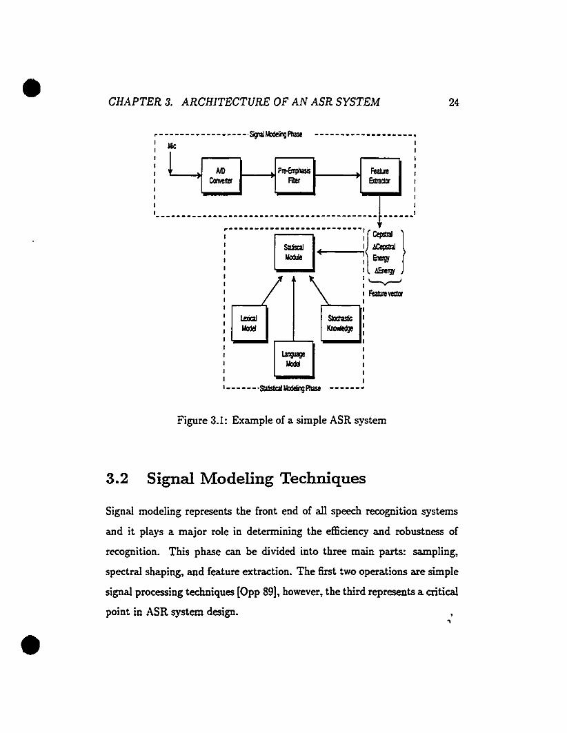
Speech recognition by machine undergoes two main phases as can be seen

from fig 3.1: the signal modeling phase in which the analogue signal is con

vertcd into a digital form, then fcd to the feature extractor that uses spectral

22

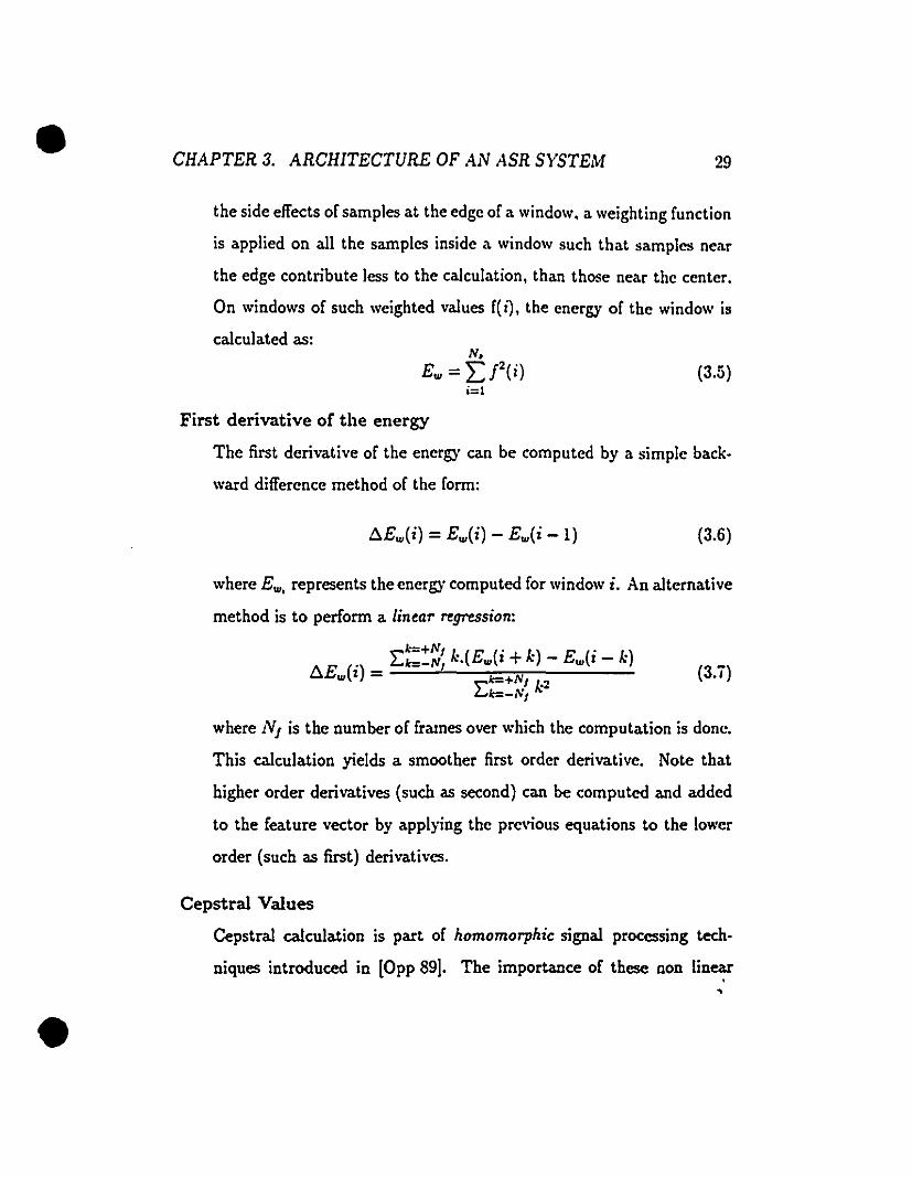
• CHAPTER 3. ARCHITECTURE OF AN ASR SYSTEM 23

•

analysis techniques to produce a parametric representation of the signal, and

the recognition phase in which statistical modeling and search techniques are

used to hypothesize the most likely word that was initial1y pronounced.

The a.im in the first phase is to extract from the input signal, features that

are similar to those used by the human auditory system to distinguish be

tween different sounds. In the second phase, the a.im is that given these

features, to determine the most likely sequence of words that was spoken.

Hence, recognition relies heavily on the feature vector produced during the

first phase: the more perceptually meaningful the features, the better the

recognition.

Chapter 1 reviewed the first building block of ASR design which is speech

generation by humans and the acoustical properties of sounds. The first part

of this chapter explores techniques by which this linguistic knowledge can

be combined to spectral analysis algorithms to produce a meaningful feature

vector. The second part reviews the statistical modeling approa.ch to speech

recognition. It is important to note here that the sections that fol1ow describe

the techniques used on Roger our ASR system at McGill University, however

there are alternative methods in both extra.cting the features (as in the use of

Linear Prediction Coding [OShaug 87)) and in recognizing the words (as in

the use of Artificial Intelligence strategies or different pattern classification

techniques [Rabi 93)).


,,111,,11

_____ ..1

Pre-Emphasist---.I Filer 1----.1ND

Converter

• - - - - - - - - - - - - - - - - - .SignaJModeIi1g Phase - - - - - - - - - - - - - - - - - - -,, Mie

: l, '----.1,,11

1 -------------------------------------

:---------@]--::----------:l=)1 _C 'ene1 1 tg{1 1 .lEnetg{1l '-v-', FeaIIn_11 ...---',.

1 leIicaI S1od1aslic: Mode! Knooleô;el '-...... ,--..1..-...... .._ .....11 l.al9J3!lll1 lIallI11

1- - - - - - •SlaIisIIcaIllodeIilg Phase - - - - - -

Figure 3.1: Example of a simple ASR system

3.2 Signal Modeling Techniques

•

Signal modeling represents the front end of all speech recognition systems

and it plays a major role in determining the efficiency and robustness of

recognition. This phase cao be divided into three main parts: sampling,

spectral shaping, and feature extraction. The first two operations are simple

signal processing techniques [Opp 89], however, the third represents a critical

point in ASR system design. ,,

• CHAPTER 3. ARCHITECTURE OF AN ASR SYSTElv[ 25

This section is divided into two part: a first part describing the proce.

dure by which a speech signal is acquired, digitized, and conditioned before

processing by the feature extractor, followcd by a second part describing the

feature extraction phase.

3.2.1 Sampling and Spectral Shaping

The first step in speech recognition is converting the incoming analog signal

into a digital signal. There are two critical parts in this phase the A/D con

version -the conversion from analog to digital- and the digital filtering

emphasizing important frequency components in the signal-.

The job of the A/D converter is to take a continuous signal and digitize it

by sampling it at regular interval and assigning signed intcger values to the

sarnples. The samples are then grouped into frames and fcd to the featurc

extractor.

In order to avoid aliasing, the sampling frequency has to satisfy Nyquist 's

Sampling Theorem [Opp 89, chap. 3J: given a bandlimited analogue signal

xe(t), then xe(t) is uniquely deterrnincd by its samples x[n] = xe(nT), n=-

1,-2,... ,+1,+2,... , if:

(3.1)

•

where n. represents the sampling frequency, while the 2!l", frequency rcpre

scnts the bandwidth of the input signal, and it is referred to as the Nyquist

rate.,

• CHAPTER 3. ARCHITECTURE OF AN ASR SYSTEM

Next, the discrete (digitized) signal is pre·emphasized by:

Si = Si - QSi_l

26

(3.2)

•

Where Si denotes a sampIe i and i ranges from 0 to the total number of

samples in a particular frame and Ct is the pre-emphasis coefficient and is

typically set to 0.95. The pre.emphasis is used to amplify spectral compo

nents above 1KHz -where human hearing is more sensitive [OShaug 87J-, thus

accentuating certain aspects of the signal that are known to be perceptually

significant .

Finally, the samples are grouped into frames which are later processed

with sliding windows to extract the features from the signal. Successive

window position overlap by typically 20% to 60% of the frame duration. De

termining a window's duration requires making a tradeo!f between short win

dows that provide better time resolution (good for detecting rapid spectral

changes) and long windows which a1low a better accuracy in the evaluation

of spectral features but smooth rapid changes.

3.2.2 Feature Extraction

There are three driving forces behind the design of efficient feature extractors:

the first is to be able to extract parameters that contain as much information

as possible about the linguistic content of the acoustical signal. the second

is that these features should be robust to variations in speakers (accent, age,

gender) and to background and channel noise, and finally the paramet~


should be able to capture the changes of the signal spectrum with time.

2i

•

As ASR systems tend to mimic the human speech production/perception

mechanism, the first trend to feature extraction techniques involved some

form of auditory modeling. The most apparent form of these features are mel

scaled parameters which are commonly used nowadays [DeMori 95J, [Young 94J

and [Ljol 94].

The mel scale maps an acoustic frequency f to a "perceptual" frequency scale

such as:f

me1,req = 25951og 1o(1 + iOO.O) (3.3)

The mel scale is often approximated as a linear scale from 0 to 1000Hz and

as a logarithmic scale beyond 1000Hz. One can thus think of eq 3.3 as a

transformation of the acoustic frequency scale into a meaningfullinear scale.

Another important set of parameters are dynamic features, introduced

by [Furu 86). which lead to a very good performance especially in speaker

independent recognition.

Other techniques have also exhibited positive effects on recognition: lin

ear discriminant analysis [Haeb 92]. [Haeb 93] and cepstral transformation,

these are used to decorrolate parameters and then concentrate useful infor

mation into a small number set of features.

Finally, in [DeMori 95) two new acoustic features are introduced by con-


sidering measurements in time domain and in broad frequency bands; both

these features increased the accuracy of recognition.

The technique used for feature extraction is the Fast Fourier Transform

(FFT) and it will be presented in the following section. The feature vector

is composed of 26 parametersl :12 me! coefficients, 12 first derivative of me!

coefficients, energy (per frame) and final!y the first derivative of the energy.

3.2.2.1 Fast Fourier Transform

The Discrete Fourier Transform of a signal is given by:

N.-lSU) = ~ s(n)e-i2,",*

,,=0(3.4)

•

where f is the frequency of the input signal, f. is the sampling frequency

and N. denotes the the number of samples per window. The spectrum of the

signal is defined as 1SU) 1.

Usually in real time implementations of ASR systems a Fast Fourier Trans

form (FFT) is used to compute the spectrum of the signal. An FFT is

a more efficient implementation (in terms of speed) of the DFT with the

added constraint that the spectrum has to be evaluated at a discrete set of

frequencies that are multiples of ft. These frequencies are called orthogonal

frequencies.

The feature vector used in our systems is composed of the follo\\;ng:

Energy of window

The energy is calculated for each sliding window. In order to reduce

IThese are the parameters use<! in our speech recognition system


the side effects of sampJes at the edge of a window. a weighting function

is applied on all the samplcs inside a window such that samples ncar

the edge contribute Jess to the calculation, than those near the center.

On windows of such weighted values f( il, the energy of the window is

calculated as:N.

E", = 2:P(i)i=l

(3.5)

First derivative of the energy

The first derivative of the energy can be computed by a simple back·

ward difference method of the form:

llE",(i) = E",(i) - E",(i - 1) (3.6)

•

where E"" represents the energy computed for window i. An alternative

method is to perform a lincar regression:

. EZ~~Z: k.(E",(i +k) - E",(i - k)llE",(z) = k=+N/ k

2(3.il

Ek=-..../

where Nf is the number of frames over which the computation is donc.

This caIculation yields a smoother first order derivative. Note that

higher order derivatives (such as second) can be computed and added

to the feature vector by applying the previous equations to the lower

order (such as first) derivatives.

Cepstral Values

Cepstral caIculation is part of homomorphie signal processing tech·

niques introduced in [Opp 89). The importance of these non lin~


sy.lems lies in the fact that by using them, one can separate the ex

citation signal from the vocal tract shape, thus providing a mean by

which the vocal tract characteristics can be extracted. As was discussed

in the fist part of this chapter, a speech signal s(n) is produced when .

air excites the vocal tract; physically this can be represented as a con

volution of the vocal tract's impulse response v(n) with the excitation

sigr l g(n).

s(n) =g(n) 0 v(n) (3.8)

Since the two signal have very different spectral characteristics they

nccd to be separated. If one can represent the signal in the log domain,

the two signais will be superimposed and thus can be separated using

conventional signal processing [Pic 93). This is how one can proceed:

First represent the signal in the frequency domain (i.e by performing a

Fourier transformation on both sides of the equation):

S(f) =G(f).v(f)

Then take the complex logarithm of each side:

(3.9)

•

/og(S(f)) = /og(G(f).V(f)) = /og(G(f)) + /og(V(f)). (3.10)

The cepstrum is defined to be the inverse transform of the logarithm

of the speech spectrum. Since perceptual frequency resolution is ap

proximately linear up to 1KHz and logarithmic at higher frequencies,

in examining the distribution of energy acf055 frequencies for relevant

,


(3.11),n =1,2,oo.,L

speech eues, the mel scale is used because, it exhibits this kind of fre

quency resolution. The mel cepstral is given by:

F 1 ~c(n) =L logIDSk cos[n(k - 2) Fl

k=O

where F is the number of filters and L the length of the cepstra1.

Usually, 24 filters are used to extract the first 12 mel cepstral values.

First Derivative of Cepstral values

The first derivative of the cepstral values can he either calculated by

a simple backward difference method as in eq. 3.6 or using a Iinear

regression over several frames as in eq. 3.;.

3.2.3 Discrete vs Continuous Models

The feature vectors can be categorized as discrete or continuous. Continuous

pararneters are the end result of the feature extraction module. Discrete pa·

rarneters can only take a fini te number of values from sorne symbol alphabet,

they are normall)' generated by applying Veclor Quanti:ation [Cray 84) on

the continuous parameters.

•

The aim of vector quantization is to reduce the arnount of data coming

from the feature extractor, by constructing a codebook (or multiple code

books) containing a distinct set of feature vectors (or codewords) that are

representative of the training data set.

During recognition, when a feature vector is produced by the feature ex

tractor module, the distance of that vector to the nearest codeword in the

• CHAPTER 3. ARCHITECTURE OF AN A5R SYSTEM 32

•

codebook is calculated and the codeword that has the smallest distance to

the produced vector is fed to the statist:cal modelling module.

To increase the efficiency of the vector quantizer, multiple codebooks are some

times used, one for each group of features extracted (so in our case one would

have a codebook for the energy, another for its derivative, a third for the cep·

stral coefficients and a fourth for their derivatives).

There are numerous considerations taken when designing a vector quantizer

such as the number of codewords, the number of codebooks, and the methods

used to initialize and train the codebooks.

A more comprehensive discussion of vector quantization can be found ID

[Gray 84], and [Rabi 93, chap. 3].

The main advantage of vector quantization is reducing the computation

complexity and thus improving the speed of the system, and its main dis

advantage is the distortion it creates which may result in poor recognition.

This distortion is due to the fact that since there is only a finite set of code

words, then choosing the ~best" one2to represent the produced feature vector

always carries a certain level of quantization errer: the greater the distance,

the higher the error. This error can be somehow reduced by having a larger

number of codewords, however it cannot be eliminated as long as there is

a finite set of codewords. This problem often leads to a tradeoff between a

large set of codewords per codebook (decrease the level of errer, but increase

complexity) and a smaller set (increase in speed).

2the one with the shortest distanee to the feature vector


3.3 Statistical Approach to Recognition

33

Speech decoding (recognition) can be regarded as a transformation from a

set of parameters (represented by the vector 0) to a sound s (where 5 can

be a word, a sub·word or just a phoneme). If the transformation yields a

sound s '" so.;g (where so.;g is the sound that was originally uttered) then

the decoder made an error.

In statistical pattern recognition, the aim is to minimize the probability of

that error, so an efficient decoder is one that chooses s such as:

s =argmax,_•• P(s 1 0)

Following Bayes Rule [Komo Sï], eq. 3.12 can be rewritten as:

P(O 1 s).P(s)

(3.12)

•

where N, is the total number of models representing the sounds of the lan

guage. P(s 10) is called the a posteriori probability of the model 5 given the

feature vector 0, P(s) is the probability of the model representing 5, and

P(Ols) is the probability of observing the feature vector given the model s.

The decoding problem thus reduccs ta solving the unknown parameters of

eq 3.13. This can be achieved by having a family of probabilistic functions

capable of containing as much information as possible about the process be

ing modeled (speech sounds in this case); thus the use of Hidden Markov

Models (HMM).

• CIfAPTEn :J. A!tCHlTECTURE OF AN ASR SYSTEM

3.3.1 Acoustic Modeling Using HMMs

34

•

Hidden Markov Modcls (HMM) are stochastic processes that modcl events

iu sequ,mec. The under!yiug assumption in the use of these models is that

the speech signal can he represented as a parametric random process and

that. t.he paramet.ers of the st.ochastic proccss can be estimated by a precise

met.hod [Rabi 88].

HMMs should he viewed as a mean of computing the similarity between a

speech signal and a recognition pattern in a statistica! manner. There are

two main advant.agcs for using these processes: first their structure (as will be

seen in the following sections) allows them to efficiently mode! the variability

of the speech signal and its spectrum with time, second the parameters that

define HMMs can be re-estimated so as best to account for the acoustical

propertics of the sounds they represent3 •

The success of statistical pattern recognition techniques, especially HMMs,

have lead to their employment in most contemporary ASR systems as in the

AT&T system [LecC 89J, the SPHINX system at Carnegie Mellon [Lee 90a],

the France Telecom system [.Jouv 94b], Roger at McGill University [DeMori 95J.

Following is a description of the structure of HMMs and the parameters that

define them. Before exploring HMMs one nceds to first explain the sim

ple discrclc Markov ModcL- and how these can be extended to form Hidden

Markov Modck

3Chapter 4 is dcdicated to the detailed description of recognition and r<-estimationmethods using IIMMs


Figure 3.2: Examplc of a Markov Model

3.3.1.1 Markov Chain

35

•

A markov chain consists of a number of states and a number of transitions

between them as can be seen from fig. 3.2. Every state represents a fixed

symbol k and with every transition between two pairs of states (5;, Sj) is asso

ciated a transitionai probability a;j. When the process starts at t = 1, every

state 5; has an initiai probability ll";. Each time a transition to astate is taken,

an output symbol is generated. For example, from fig 3.2, if one goes from

state 1 to 2, at time t, the output symbol "blue" is generated. By the same to

ken, ifone observes the sequence of colors 0 = blue red red white blue white,

then one can trace back the sequence of states that produced it; in this case,

it will be 525151535253.


•

In these types of models, each observatic.n is considered to be independent

of ail the previous observations except for the one that immediately precedes

it, so that aij denotes that the system was in state Si at time t and made a

transition to state Sj at time t+1.

The model described above is constrained by the fad that each state

represents a predetermined symbol, so if one wants the Markov chain to

generate a 100 symbols, one needs a model with a 100 states, this is dearly

unrealistic in applications where numerous observation symbols are needed

as in the case of speech recognition.

3.3.1.2 Hidden Markov Models

A practical solution to the problem stated above, is to make the observation

symbol a probabilistic function of the state. In this fashion, aIl symbols are

possible at every state, each with its own probabiIity. This method means

adding one more parameter to the Markov model described above: an NxM

matrix where N denotes the number of states in the model and M the number

of observation symbols. This matrix is referred to as an observation symbol

probability matrix B and it can represent any number of observations. Each

element of the matrix , say bl2 represents the output observation probability

of the 2nd symbol in state 1 (this can aIso be denoted as bql(02 ) •

Such models are called Hidden Markov Models (HMM) because they are

doubly embedded stochastic processes in the sense that not only are transi

tions between states probabilistic, but the output symbol observed at each

state is aIso determined by a probability output function. Using the example

• CHAPTER.1. ARCHITECTURE OF AN ASH SYSTEM

of fig 3.2, if an Hl\U...l is lIscd to reprcscnt the colors. th('11 ('i\cll sta!.l' \\'olll~l

he able to rcpresent ail thrcc colors, rathcr t.han IHwillg olle rulor for {'"ch

sate. In this contcxt by going from S, to 8'2, Olll' rould pI'O(II1('(' \'('d, bllll' or

white dcpending on thc highcst output probabilit.y of stat.{' ....·2.

3.3.1.3 Parameters of an HMM

DÎ~crete"HMMs(in which the output distributioll fllllCt.ioll rt'pn's('nts a dis

crete symbol k) can be described bya sel of N states (a st.at.c that. is reaclwd

at time t is denoted by qt). and a set of Al output. observation sj'llI1>ols il."SOCÎ

ated \Vith l'very st.atc (these can be reprcscllted by V = [1'10 1,2•...• l'M]). TIlt"

observations correspond to the physical output of the syst.em 1>cing tIlodcbl.

An observation veetor is sometimcs denoted (\.... 0 = 0, Q.~ .. . 0]' wlwrt' 01 is

the symbol generated as time 1 and it is one of the symhols of tlll' st'l V. '1'

l'l'presents the total number of observations generatcd.

An HMM has can be defined by its thrcc paramcters:

1 The initial output probability associatcd \Vith each statc. This can I)(~

described as the probabi1ity that the system is in statc S, at timc 1 = 1:

"i =P[ql =Sr] (:1.1,1)

•

4Continuous IIMMs have a dilTerent output distribution [uncliQu anJ ar'~ dis~IIs.'if·,1

later


2 An NxN statc transition matrix representing the transitional probability

for cvcry pair of states, it is given by:

A= (3.15)

A transition aii corresponds to the probability of making a transition

to state Si at time t+l given that the system was in state Si at time

t, this can be represented as:

(3.16)

4 An NxM observation symbol probability distribution matrix B such as:

B= (3.li)

The output distribution symbol probability bj(k) is the probability that

the system is iù state Si and that symbol k is observed, this can be

reprcsented as:

•

1 ~j ~ N

l~k$.M

(3.18)

(3.19)

• CHAPTER 3. ARCHITECTURE OF AN ASR SYSTEj',J

3.3.1.4 Structure of an HMM

39

•

Another important consideration is the structure of HMMs used in speech

recognition. The model described in fig 3.2 is called an ergodic model be

cause every state can be reached from every other state; however, for HMMs

to properly model the time varying speech signal, transitions from states with

higher indices to states with lower index should not be allowed (i.e moving

backward in time), thus the use of /eft-to-right models as described in fig 3.3.

Figure 3.3: A five state, left-to-right HMM mode!

ln left-to-right models states are conneeted in a sequential manner, and

each state, except the last. is connected to itself to rel!eet variability in time

(since difl'erent instantiations of phonemes and words can rcgister at difl'ercnt

times), the last state is called a sinkstate and it denotes the end of the model.

The number of states in a model is usually chosen to denote the duration

in time of the process being modeled, for example in phonemic HMMs it is

common to choose 3 state models, state 1 representing the left part of the

phoneme, state 2 the middle part and state 3 the last part. Of course there is

no set rule as to how many states should be used, however an increa.se in the


number of states means an increase in the complexity of the computations.

Usually, there is one HMM for every process being modeled, so in phone

mic HMMs, there wiII be one HMM to each phoneme used. However when

phonemes in context arc modeled, elusterin/techniques are used to reduce

the number of phonemes needed [Jouv 94a] [Ljol 94] [DeMori 95].

3.3.1.5 Types of HMMs

Finally, there arc dilfercnt types of HMMs that can be used for recognition

depending on the type of feature vector presented by the feature extractor.

The main dilferencc betwccn dilferent types of HMl\Is lies in their output

distribution function bO.

Discrete llMMs using one codebook

The observation symbol prohability b(k) must satisfy:

k=.If

L b(k) = 1k=l

(3.20)

whcre k is a symbol of the alphabet and M is the total number of sym·

bols. The output discrete distribution function can thus be exprcssed

as:

b(O) = P(O 1 k) k E V (3.21 )

•

Discrete HMMs using multiple codebooks

The output discrete distribution function is the product of the distri·

bution functions associated with every codebook. 50 if there are Ne

'Clustering will be diocuosed in chapter 6

• CHAPTER :J. ARCHITECTURE OF AS :ISIl SYSTE.\1 ,II

codebooks, and for ('ach codl'!lOok w(' bav(' an output oh,,'rval;ou v,'''·

lor Oc lhen:r:.\'r

b(O) = II 1',(0" 11.')~=I

( '1 "")...-

where 0' is lhe ct!· C0ll1l'0ll<'nt. of 0 and (F E (J, 1.... , /\'" - 1 wi!t'n'

K, is t.he size of codebook c.

Cou/irlltous UMMs usi1l9 Multit'(lri,,/r: G(III""i,," ,{('1I,'i/y juurlioll,'

A continuous out.put probahility has to satisfy:

Jb(O)'{(O) = 1

A multivariate Gaussian distrihution funclion is giv('n hy:

b(O) = (:I.:!'\ )

•

where N is the dimension of the feature vcclor (:!G in our '·'LSl'), Il, is

the mean vector. and L:~ is the covariance rnatrix.

However. phonel11<'S arc poorly cstil11atcd hy IlMl\1s with on,· l'df l','r

transition. thus the use of a finite mir/lIN:.' of Gaussian d.'nsiti.", [N.·y 881.

The mixture distrihution is a weight('<\ surn of Nk .Iistrihutions:

k=N" k=N"

Pmir(O) = L It'k.Pk(O).snch a~ L "'k = 1 (:I.:!!i)k=1 k=1

These mixtures arc usually il11plel11ented hy having ""v('ralparalld t.ran·

sition betwccn two statcs. cach transition having a Ganssian ,Iistrilm·

tion function.

Scmi-Continuous lB/Ms

Semi-Continuous HMl\ls arc hybrid modcls that inlt~ratediscrete proh

abilities with continuous densitÎ<'S in an effort to comhine SIX....~J with

• CIIAPTEJI. :1. MlCJlITECTURE OF AN ASR SYSTE,H 42

•

accuracy respectivcly. In these modcls, a set of continuous densities is

s/lllrcd by ail discrete output distributions [Huang 89].

3.3.2 Using HMMs for 'fraining and Recognition

3.3.2.1 Overview of Training

BcCore performiug recognition one first nccds to use sorne training algorithm

that can estimate the parameters of the HMM modcls from a training data

sd, which should normally contain a large number of sentences that are rep

resentative of the words the system will be expected to recognize.

First step in training is listening to the training sentences and writing the

sequence of words that form thcsc sentences. This is callcd transcribing. Each

distinct word is then placcd in a /cncon with its phonemic spelling. Usually

for more efficient training, multiple pronunciations of the same words are

a1so put in the lexicon to provide as much information as possible about the

word.

Once the transcription and phoneme labelling is done, the training sentences

along with the text speech and lexicon arc fcd to a training algorithm that it

erativcly rc-cstimates the parameters of H1\!:\ modcls each time maximizing

the likclihood that indccd the training speech sas produced by theses mod

cls; this estimation method is bascd on the Baum·Wclsh a1gorithm [Bau 72)

and is fully dcscribcd in chapter 4.

Sometime the data is labeUed more prccisely such that a sentence is segc

lIIeu1<-'<1 into timesequeuces (i.e a set of samples) each representing a phoneme•

• CHAPTER 3. ARCHITECTURE OF AN A.SR SYSTEM 43

•

When the training algorithm uses this time alignment. the training is called

segmented training and it is usually used in the first iterations of the training

procedure to properly initialize the parameters of the modc1s.

3.3.2.2 Overview of Recognition

Once the parameters of the HMMs arc properly estimated, the recognition

can be donc using the test sentences. However, one first needs to build il.

grammar that describes how words are connected. The role of the gram

mar, as in the case of human speech perception, is to impose as set of con

straints on the sequences of words. In HMMs, statistical grammars, called

n-gmm grammars, are provided that define the probability of occurrence of

phonemes. There are different types of grammars, such as bigrams that gives

the probability of ail pairs of phonemes (or words), and trigmms that give

the probability of ail triplets of phonemes (or words).

Once the grammar is built, the recognition process can begin. This pro

cess, in its most simplistic form, is a large scarch among ail the phoneme

(word) models for the ~best~ word (phoneme) sequences that can describe

the observed feature vector. However sucb a method would require an exces·

sive amount of computation. More efficient techniques have been devc10ped

such as the Viterbi alogrithm [Vite 6i) which is also fully described in the

following chapter.

•

•

Chapter 4

Training and Recognition

Algorithms for HMMs

4.1 Introduction

The previous chapter explained the architecture of automatic speech recog

nition and Hidden Markov i'>lodcls (HMM) were melltioned without any

details about the mathematical foundation underlying their use.

This chapter presents an overview of the fundamental problems for HMM de

sign. and focuses on the search algorithms that allow us to use these models

during the recognition phase, and on the training algorithms during which

the parameters of the HMMs are re-estimated 50 as to best account for the

observed training data set.

In the folIowing sections it is assumed that the reader has some prior

knowledge of HMMs and their use in speech, however, if this is not the case,

44

• CHAPTER 4. TRAINING AND RECOGNITION ALGORITHMS 45

sorne introductory references are recommended such as [Rabi SS], [Rabi 93,

chap.6], [VAl 91], and [Pic 90p This chapter is divided into five main sections,

first the three main problems of HMM design are described, next the solution

for each of the problems is given in a separate section, and fina.lly sorne

implementation issues concerning HMM design are presented.

4.2 The Fundamental Problems for HMM

Design

Given a left-right HMM such as the one in fig 3.3, there are three basic

problems that have to be solved in order for these models to become useful

for rea.l time applications like speech recognition.

Suppose an observation sequence is given by:

And suppose an HMM model À is represented by:

À = (r.,A,B)3

Then one can define the three problems as:

(4.1)

(4.2)

•

Problem 1- Given the <"'5ervation sequence 0 and the model À, what it

the probability P(O 1À), ie. what is the probability that the sequence

Ois observed given the model À?

IThe theory and algorithms presented in these rererences are summarized in thischapter.

'where T is the length of this output sequence3As discussed in chapter 3, this representation ofan HMM. means that the model ~ has

an initial probability matrix ". a transitional probability matrix A. and an observationprobability matrix B•

• CllAPTEn 1. TRAINING AND RECOGNITION ALGORITHMS 46

Problem 2- Civen the observation sequence 0 and the model À, and sup

pose that the state sequence of the modcl Àis defined as Q = 'Il '12' .. '1T,

then what is the olJtirnal state sequence given the observation sequence?

Problem 3- How does one adjust the parameter À= (r., A, B) of an HMM

so as to rnaximi=c l'(O 1 À)?

Finding the solution to problems one and two means identifying how recogni

tion can be done using HMMs where as finding the solution of problem three

permits one to train the modcls so that they can best represent the observed

data set [Rabi 88].

4.3 Problem l:Calculating P(O 1 >.)

4.3.1 Basic computation

Civen a model À = (r., A, B), with a fixed state sequence of length T,

Q = Q1Q2'" QT and an output observation sequence 0 = 0 10 2... OT,

then one can easily compute l'(O 1 À) by summing over ail possible paths

q in the mode! À, the probability P(O 1 Q, À) (which is the probability of

observing the sequence 0 given the state sequence Q in the model À) multi

plied by the a priori probability P(Q 1 À). Thus,

•

l'(O 1À) = L P(O 1Q,À)l'(Q 1À).1lQ

(4.3)

• CHAPTER 4. TRAINING AND RECOGNITION ALGORITHMS 4i

However, we already know that the probability of an observation sequence

0, given a state sequence Q and a model À can be represented as:

(4.'1 )

The probability of the state sequence Q is given by:

(4.5)

Thus, we can rewri te P(°1À) as:

P(O 1À) = L 1l"qlbql(0t!aqlq2" .aqT-lqTbqT(OT) (4.6)qlq2...qT

Since eq. 4.6 is a sum over ail paths in a mode!. and since the number

of paths increases exponentially with the length of the observation sequence,

then if the model has N possible states that can be reached and the obser

vation sequence is of length T, the order of eq 4.6 becomes 2.TNT • So

even for very short observation sequences Iike 50 and with only 4 states, this

procedure would need 2.50.-150 or around 1032 computations, this is cIearly

unfeasible in real time applications.

Fortunately, there are recursive algorithms that have been deve!opcd

which make the calculation of P(O 1 À) both simple and efficient. One

such algorithm is called the forward-backward a/gorithm [Bau i2).

4.3.2 The Forward-Backward Algorithm

Consider the forward variable Cl'I(i) and the backward variable !J1(i):

•Cl't(i) - P[0102'" Oh qt =S; 1À)

!Jt(i) - PiOt+IOI+2 ••• OT, qr = Sol À)

(4.i)

(4.8)


Ol(i) reprcsents the probability that the model ,\ produced the partial

output observation sequence 0 10 2 •• • 0, until time t, using a transition se

quence that ends at state Si. BI ( i) reprcsents the probability that the model

,\ produced the partial output observation sequence 0 1+10,+2", OT, given

that the first transition in the generated sequence started from state Si. To

state it differently, Ol(i) is the joint probability that the output observa·

tion sequence 0 = 0 102" .0, is generated and we stop at state Si at time

t, and /3,( i) is the joint probability that the output observation sequence

o =0 1+10 1+2 " • OT is generated and we start at state Sj at time t.

Both of these quantities are normaIly calculated by creating a trellis (refer to

fig 4.1) in which the tlh column corresponds to time t and the ilh row corre

sponds to state Si in the HMM mode!. They are both computed recursively,

column by column, 0,(i) starting from column 0 and moving forward in the

treIIis and /31(i) starting from column T and mO\'Ïng backward in the treIIis.

The recursive algorithm for Oi and /3i is given by:

LInitiali:ation :

o,(i) =l3T(i) =

2.Recursion :

1,

1 $ i $ N

1 $ i $ N

(4.9)

(4.10)

•

0 1+1 (i) = [E~I ol(i)aij)bj(Ol+!), 1 $ t $ T - 1

1 $i $ N (4.11)

P,(i) = Ef.,1 aijbj (0'+1 )PI+! (i), t = T - l, T - 2, ... ,1

l$i$N (4.12)


In step 1, Q,(i) is initialized as the joint probability that we are in state Si,

and observing 01> while th( i) is arbitrarily set to 1 for ail N states in the

HMM mode!.

In the recursive step for the forward probability, since Ql(ij is the joint prob

ability that the output sequence 0 10 2 ••• 0, is observed up to time 1and that

we are in state Si, then by multiplying Q,(i) by the transitional probability

aij, we get the joint probability that the output sequence up to time t is ob·

served and that we have made a transition to state Si at time 1+1 from state

Si. By summing the former product over ail N states, we get the probability

of state Si at time 1+1 with ail the previous ~U,put observations, up to time

1. Now that Si is known, then to lind Q,+I(i), we need to multiply Si by the

output observation at time 1+1 for that state, which is nothing but bi(OI+l)'

Note that in order to solve for P(O 1..\), ail what needs to be done is to sum

ail terminal for'\Vard variables QT(i). Hence,

N

P(O 1..\) =L or(i).i=l

(4.13)

•

Calculating P(O 1 ..\) using eq. 4.13 is of the order N2T, 50 going back

to the previous example, if there are 4 active states and 50 observations,

this procedure needs 4250, or 800 computations, comparing it to l()32 as was

obtained using the straightforward calculation of P(O 1À), we saved arouno

29 orders of magnitude.

Similarly. the recursive step of the backward probability shows that in order

to have been in state Si at time 1and to account for ail output observations


startiog at t+l on, we have to take ioto considerations all possible states Sj,

aL Lime t+l, and accounL for all transitions from Si to state Sj (using the aij

term), along with the observation at time t+l in state Sj (thus the bj(Oe+l

term) and finally multiply it by all the remaining output observations from

statc Sj (thus the Pt+IU) term).

Both the forward and backward variables play a key role in search and train

a1gorithms as will be seen in following sections.

state

i

2

1

1 2 3 4

observation

... ..

......

.....L

•Figure 4.1: Example of a trellis. adapted from [DeMori ]


4.4 Problem 2:Finding An Optimal Path

There are many ways one can interpret fin ding the optimal path given an

output observation sequence, and a mode! À. One can for examp!e, choose

the optima! path to be the one that maximizes the expected number of cor

rect individual states. However, this cannot be applied to speech recognition

because in ma;'(imizing individual states, one might end up with a state se

quence in which one or more states are not connected.

What is needed in speech recognition is the ability to determine the best state

sequence given an observation sequence 0 and a mode! À, in other words a

way of maximizing P(Q 1D,À).

Such a technique was developed in 196; by Viterbi [Vite 6;), and is referred

to as the Viterbi Algorithm. Following is an overview of this algorithm.

4.4.1 The Viterbi Algorithm

Givpu a trellis such as the one described in fig 4.1, the Viterbi algorithm

computes the lowest-cost path, where the cost of a path at a certain node in

th,; t.el.lis ti is given by the sum of the cost at the previous node ti_1 and the

cost of goillg from ti_1 to ti.

In order to view how this algorithm is structured, let us define

(') _ Q,(i)P.(i)

l' 1 - P(O 1À) (4.14)

•as the joint probability of being in state Si at time t and observing the output

sequence O. Note that the P(O 1À) in eq. 4.14 is a normalization factor that

makes 1.(i) a conditional probability, such as the sum over ail N of al!.ys at


time t is 1. Note also that the value of P(O 1..\) can now be calculated using

the forward variable alti) as stated in eq. 4.13.

To find the lowest·cost path (or best state sequence ql q2 ••• qT) in the trellis,

given an output observation sequence 0 10 2 ••• OT, we define ét(i) to be the

best score along a certain path in the trellis, at a given time t, that can

account for the output observation sequence up to time t and that ends at

state Si:

From eq. 4.15, one caon ca.lculate the lowest·cost path recursively by:

(4.16)

4.4.2 Recognition Using the Viterbi Algorithm

During recognition, one a.lso needs to keep track of the state Si that had the

maximum él(i) at time t. Once the last observation is reached at time T,

recognition is performed by backtmcking through the trellis, extra.cting those

states that maximized cSt(i). 50 for recognition using the recursive Viterbi

a.lgorithm one needs to define two arrays, one to hold the maximum cSl(i) and

one to hold the corresponding state Si. The a.lgorithm is described as:

1. InitiaIi::ation :

•

él(i) = r.jbi ( Od, 1 ~ i ~ N

III/(i) = 0

2. Rccursion:

(4.1i)

(4.18)


l$.j$.N (4.19)

1II,(j) = argmax 'S'SN [0,-1 (i)aijj, 2$.t$.T

l$.j$.N (4.20)

S. Termination:

po = max [OTt il] (4.21)IS'SN

qi- = argmax [oT(i)] (4.22)lSISN

4. Backtrad:ing:

q; = 1II,+I(q;+\), t = T - 1, T - 2, ... ,1 (4.23)

The array 1II,(j) holds the index i of the S'_I(i) that maximizes S,(j) ac

cording to eq. 4.19, it is basicaily a pointer to the best preceding state Si.

After the last output observation at time T, p. and qi- will contain the high.

est vaiues of 0,( i) and the states that produced this maximum respectively.

•

Sometimes, wcights can be imposed on transition~ and observation prob

abilities to increase their contribution during the search process. These

weights arc referred to in the literature as Language Madel Weights. For

example, if one wishes to increase the transitionai probability contribution,

then instead of using aij in eq. 4.19, one would use (aij)w, whére Wis a pre

specified weight. In sorne recognition systems ~ , language models weights are

used on transitionai probabilities from one phoneme model to another, rather

than on transitionai probabilities between the states of a model. Language

~As the one developed in the speech lab at McCiIl University

•

•

CHAPTER 4. TRAINING AND RECOGNITION ALGORITHMS 54

model weights and their effects on recognition will be reviewed more closely

in the in chapter 6.

The essential calculation in the Viterbi algorithm lies in eq. 4.19: the only

path that gets propagated is the one that has the highest probability among

all the paths that can make a transition to the current state at time t. How·

ever, although the optimal state sequence is the most likely path through the

models, the sequence of models that correspond to this path may not be the

optimal one. This is due to the fact that the probability of a model sequence

must be summed over aU paths in the sequence, and not only the most likely

path. Nonetheless, in most cases, the most likely path does provide a good

~d efficient approximation.

The last point to make here is that although this algorithm reduces the

search space by propagating only the most likely path at a particular time

t, it still imposes a considerable amount of computation on the recognition

process resulting in large response times in real time applications. However,

some adjustments cao be made to the algorithm to increase its speed; this

leads to the next topic: the Viterbi Bearn Search.

4.4.3 The Viterbi Beam Search Aigorithm

In most real time applications, the response time plays a key role in mea.

suring the efficiency of the system. In automatic speech recognition systems,

due to the comple:<ity of computations, speed becomes a critical point in the

•

•

CHAPTER 4. TRAINING AND RECOGNITION ALGORITHMS 55

design strategy.

One way of improving the speed of the system is to limit the search space

of the Viterbi a1gorithm. This can be achieved by rcstricting the search to

those trellis nodes that have a Iikelihood (or probability) greater than some

fraction of the maximum likelihood in the given column of the trellis. This

technique is called Bearn Search, and following is a brief description of how

it is implemented, more details can be found in [LeeC 89].

Given the trellis as ;n fig 4.1, each time a trellis column t is computed, the

value ptmaz of the highest probability of any node in the column is found.

Then, only those nodes with a probability greater than Pt"az - 6(t) will be

kept in the list of active nodcs, the rest of the nodes are pruned or disre

garded. 6(t) is a preset thrcshold, it is referred to as the beam width. As the

computation time in the Viterbi a1gorithm is proportional to the number of

active nodcs in the trellis, then it is clear that the width of the beam will

have an effcct on the speed of the a1gorithm; needless to say that a smaller

width means less active nodcs and thus higher speed. However, there is no

general relationship between the beam width and the computation time, in

some experiments it was reported that computation time increased expo

nentially with 6(t), while others reported an a1most linear increase for large

vocabulary [LeeC 90].

•

•

CRAPTER 4. TRAINING AND RECOGNITION ALGORITRMS 56

4.5 Problem 3:Estimating the Parameters of

anHMM

The previous sections described solutions to the problem of recogni:ing a

speech signa.! by finding the most likely set of models that could have pro

duced the observation sequence generated by that signa.!; however, nothing

was said on how the parameters of these models were initia.!ized and esti

mated so as best to account for the observed input speech signa.ls. This

section reviews how HMM models are created and how their parameters are

iteratively re-estimated, this is referred to as training the HMM models.

There are many training techniques, the most commonly used is the Max

imum Likelihood Estimation (MLE) method, a.!so referred to as the Baum

Welch or FOnDard-Backward re-estimation method [Bau ;2], [Lip 82]. Oth-

ers techniques have becn developed such as the segmental k-means training

[LeeC 90], the Maximum Mutual Information (MMl) estimation [Bahl86],

[Chow 90], the Minimum Discrimination Information (MDI) estimation [Eph 89J,

and Corrective Training [App 89]. Following is a description of the MLE

method.

4.5.1 Maximum Likelihood Estimation Method

ln MLE training, one tries to adjust the parameter (A, B, 11') of and HMM

model À 50 as to maximize the probability of the observation sequence gen-

• CHAPTER 4. TRAINING AND RECOGNITION ALGORITHMS 5i

erated by the training data. The following estimates of the parameters arc

proposed:

ii7 = Expected no. of times in state Si at t=1 (4.24)

al) = (Expected no. of transitions from state Si to state Si)Expected no. of transitions from state Si

(4.25)

(Expected no. of times in state Si and observing symbol k)Expected no. of times in state Sj

(4.26)

Next, one has to define the joint probability e,(i,j) of observing the se

quence 0 = 0 10 2 , •• 0, and being in state Si at time t and making a transi·

tion from Si to Sj at time t+l. However, the joint probability of observing

the output sequence 0 and being in state Si has already been calculated in

the 'Jiterbi algorithm (eq. 4.14), so one can calculate e,(i,j) bymultiplying

the joint probability of observing the sequence 0 and being in state Si at

time t by the transitioniJ probability aij and the output observation at time

t+1 of state Si which is nothing but bj ( O,+d, this gives:

(4.2i)

•

Hence, the expected number of transitions from state Si to Sj is nothing

but the sum o"er t of e,(i,j). Moreover, if one sums il(i) of eq. 4.14 over

time t, one gets the expected number of times the state Si is visited or in

other words the expected number of transitions made rrom Si. Wc cao thus

•

•

CIiAPTER 4, TRAINING AND RECOGNITION ALGORlTIiMS 58

v.':oite:

T-l

L e,(i,j) - Expected no. of transitions from state Si to Sj (4.28).=1

T-I

L "(.i = Expected no. of transitions from state Si (4.29).=1

The estimation formulae for the parameters of the HMM mode! can be

rewritten as:

if = "(I(i)

(4.30)ET-1e(" ')

ai) = .=1 • Z,}

E T- I (').=1 "(. Z

(4.31 )

bi(k)ET,.. "(t(i)

= 0,··1rE;"I "(.(i)

(4.32)

Thus the MLE method can be implemented as a recursive procedure such

as:

1./nitiali:alion:

Consider a mode!..\ 'vith initial values,..\ = (r.,A,B)

!!.Recursion:

Use the previous values for ..\, A and B in the right hand side of equa

tions 4.30,4.31 and 4.32 to CI)mpute new parameters X=(r.,A,Ë) as

determined from the !eft hand side of equations 4.30, 4.31 and 4.32.


If P(O 1X) ~ PlO 1.\), then the new model Xis better than the old

one, so reset the previous values to those obtained in this iteration and

repeat step 2. Eise Stop.

3. Termination:

Model Xdefines a critical likelihood such as X=.\. At this stage one

has reached the maximum likelihood estimate of the model ,\.

4.5.2 MLE Method with Multiple Sentences

As was discussed in chapter 2, left to ri9ht models are mostly used in speech

recognition because of their ability to refiect the temporal changes in an

incoming speech signal. However. the major drawback of these models is that

their structure makes it very hard to accurately re-estimate the parameters

with only one observation sequence (or one sentence). This is due to the

fact that only a small number of observations is usually associated with each

state. To overcome this problem, the training algorithm discussed in the

p.evious section is extended to include multiple training sentences.

In this case the observation vcetor 0 bceomes:

(4.33)

•

where L is the total number of sentences and each sentence v has its own

observation vcetor O' =O\')O~') ... O~).

It is assumed that each observation sequence is independent of ail the others.

In this case, the parameters of the HMM model are only estimated after

aIl the sentences have been processed. this leads to the following estimation

•

•

CIiAPTER 4, TRAINING AND RECOGNITION ALGORITIiMS 60

formulae:

if 1 t V") (4.34)= L i1,1\/=1

LL LT-1~V(' ')ai) = 1,=1 t=1 t l,)

LL LT- 1 V(')0=1 '=1 i, 1(4.35)

L:=I LT,., irUlbj(k) or··.- LL LT V( ')0=1 '=1 i, J

(4.36)

Fig 4.2 presents the f10w diagram of the training procedure (adapted

fnm [VAl 91)). Usually, to see if the models have reached their maximum

likelihood, a recognition test is done using the newly estimated parameters.

If the error rates drops, it means the new models have improved over the

last ones. Training is repeated until the recognition with the new estimated

models doesn 't improve.

•

•

CHAPTER 4. TRAINING .-\ND RECOGNITION ALGORITHMS 61

initial modeli.(A,B.Jt)

use the previousmultiple indcpendant modcl i.(A.BJt) to

observations ...-~ estimalC aNEWmodel Â,'CA',B'.7t')

no

rcached maximumlikelihood

Figure 4.2: Training \Vith multiple observations


4.5.3 Estimating the Output Distributions ofa CDHMM

So far, the discussion on parameter re-estimation has evolved around dis·

crete HMMs. The estimation formula for the output distribution vector B

(eq. 4.32) relies on observing a discrete symbol J( from a finite alphabet, thus

the use of a discrete probability density at each state of the mode!.

However, as was mentioned in chapter 3, there are other types of HMMs,

mainly those that use continuous output distributions rather than discrete

ones (continuous density Hidden Markov Models or CDHMM). As was

stated in the previous chapter, CDHMM have the advantage of being able

to model more precisely the continuous speech signal, especially when one

associates which each state a weighted sum, or mizture of Gaussians. This

sections examines the estimation formula for the parameters of a CDHMM

that uses mixtures of multivariate Gaussian distributions.

Let us first represent an M-mixture Gaussian output distribution by,

M

bj(O) = L c;kN(O,iJjk, Ujk)/r=1

(4.3ï)

•

where 0 is the observation vector extracted from the input signal and N is

a Gaussian density function with mean vector iJ and covariance vector U.

The tenn C;k represents the gain of the k'h mixture of state Sj. The sum

over all K's is used to represents ail the mixtures associated with state Sj'

The mixture gain in eq. 4.3; has to satisfy the constraint that the sum of

all mixtures for astate Sj is one, 50 that the probability density function is


properly normalized:

1+00

-00 bj(O)dO = 1 1 ~ j ~ N. (4.38)

Suppose there is a CDHMM composed of an M·mixture Gaussian density

function with JI = 6. It was shown [Rabi 93J, that the mixture gains Cik for

astate i, can be interpreted as transitions to substates i b i2• i3• i4, is, and i6

with probabilities Cib Ci2. Ci3. Ci4. Cisand Ci6 respectively, with each transition

having its own mean /lik and covariance Uik • Then each substate makes a

transition to astate io called a wait state with probability LIt was proven

that this composite set of substates, each having a single density function

associated with it, is mathematically equivalent to the mixture density func

tion associated with a single state. Thus, the estimation formula.e for the

para.meters of the mixture Gaussian density become:

Cjk =

/ljk =Ei:1 Î,(j, k).Ot

Ei:1 Î,(j, k)

(4.39)

(4.40)

(4.41)

Ujk =

•

Ei:1 Î,(j,k).(Ot - /ljk).[(Ot - /ljk)Tj

Ef:l Î,(j, k)

The T in (Ot - /ljk)T denotes the transpose of the matrix. Note that

here, Î,(j, k) represents the probability of being in state Sj at time t with

the k'h mixture component a.ccounting for the observation vector 0,.

As far as the estimation for Ti and <lij, the sa.me formula.e derived for the

discrete HMM ( eq 4.32 and eq. 4.30) ca.n be used for continuous HMM•

• CHAPTER 4. TRAINING AND RECOGNITION ALGORITHMS

4.6 Implementation Considerations

4.6.1 Initializing the HMM models

64

•

There is no set rule as to how to determine the initial values of the HMM

parameters (11", A, Bl, however our experiments along with others [Rabi 89),

have shown that these initial values play a major role in determining the per

formance of the models during recognition. As was discussed in the previous

section, training is an iterative process that should eventually converge to a

local maximum. The initial values of (11", A, Bl determine which maximum is

reached after training.

In [Rabi 93], it is also suggested that the initial values for the transitional

probability matrix A and the initial probability matrix 11" can be safely cha

sen randomly, but the values of the output distribution matrix B, especially

when using continuous density CDHMM have to be selected with care. There

are many techniques developed to initialize the output distribution matrix

such as the use of hand scgmented data to bootstrap the models. linearly

segmenting the training data into their corresponding distribution sequence

and then using all frames that correspond to a given distribution to estimate

the initial values [LceC 90J, the use of segmental k-means segmentation with

clustering etc... .

4.6.2 Insufficient Training Data

Insuflicient training data is considcred one of the most challenging problcms

in real time realization of speech recognition systems, especially in recent

•

•

CH..l.PTER 4. TRAINING AND RECOGNITION ALGORITHMS 65

years when the usefulness of Contc:rt Dependent Modcls emerged 5 and re.

searchers were faced with the problem of insufficient training data, and lim·

ited machine resources to train model~ in context.

Experiments dearly show that the larger the training set, the better the

models and the higher the recognition. Anoth~r important issue is the rep·

resentati"eness of the given training set, the more varied the set (in terms of

variations in acoustic featurcs such as gender, accents, age, context, etc ... ),

the more robust the modcls are.

In cases where the training data is too small. the output observation matrix

becomes mostly filled with zero probabilities. As it was shown in previous

sections, the estimation of bj(k) relies on the joint probability of observing a

symbol k and the expected number of time we are in state Sj, 50 if there is

no occurrence of symbol k, bj(k) is set to zero and will always remain zero.

This problem is more evident in CDHMM using multiple mixtures because

of their complex structure and usually large number of distributions. In

most cases. researchers tie mixtures together 50 as to reduce the computa

tion complexity and provide more training data to estimate the parameters

[DeMori 95J.

Experiments show that the more training data is provided, the more fea·

tures (i.e more observation sequences) are induded in the training procedure.

the more robust the system becomes. Poor performance is observed when the

data used during recognition produce features that were never encount{:red

during training.

'Context Dependent Models will be discussed in details in chapter 5 &: 6


4.6.3 Underflow Problems

The problem of using HMMs is that often, the probabilities calculated during

recognition and training tend to approach zero exponentially with time, this

causes these pararneters to attain values that excccd the precision range of

any machine, resulting in an underflow problem. A remedy to this problem

is the use of scaling and logarithmic calculation.

Calculating the logarithm of the probabilities leads to a more efficient com

putation both in solving the underflow problem and eliminating the U:le of

multiplication and division (which arc expensive in terms of speed). As we

rccall:

log(r.y) = log(x) + log(y)

xlog(-) = log(x)-Iog(y)

y

(4.42)

(4.43)

•

50 by considering the logarithm of probabilities one can increase com

putation spced considerably. However, one cannot compute the logarithm

of probabilities when their computation involves summations such as in the

forward and backward calculations (eq. 4.12 and eq. 4.13). In thcse cases,

scaling is applied to the variables [Rabi 93] .

•

•

Chapter 5

State of Art in Speech

Recognition

In this chapter, sorne of the recent developments that have played a major role

in promoting the use of continuous, speaker independent ASR systems are

explored. The following sections describe sorne of the new ideas and methods

that proved to have a positi\Oe effect on the accuracy and robustness of these

systems; needless to say, that these ideas wouldn 't have had this impact

hadn't it been for the constant improvements in the hardware technology

and the Iow cost of memory which makes these system run in real-time and

provide the proper environment for their implementation.

6;

•

•

CHAPTER ,5. STATE OF ART IN SPEECH RECOGNITION 68

S.l Availability of Large Training Data Sets

As was discussed in chapter 3, one of the critical points in the training proce

dure is to have a large and representative set of sentences. The more features

the HMMs are exposed to, the better the parameters are and the higher the

recognition accuracy.

Nowadays, large (such as the Wall Street Journal corpus, 20,000 words),

medium (such as the Air Travel Information Service, 1800 words) and small

(such as the Ti connect·digit corpus, 10 sentences) speech corpora are avail

able to use by all researchers, mainly due to the Advanced Research Project

Agency or ARPA efforts, [Makh 94J.

Another common medium speech corpus, and the one used in the experiments

in this thesis, is the DARPA TIMIT Acoustic Phonetic Speech Corpus. The

TIMIT corpus was a combined effort between Texas Instrument (TI), the

Massachusetts Institute of Technology (MIT) and Stanford University.

The availability of these speech corpora meant that performance of different

ASR systems could be compared using common test beds.

S.2 Channel Noise Reduction

Channel noise, specially over telephone lines, alters the features of the speech

signal thus causing performance to drop. One of the new methods developed

at France Telecom [Mokb 94] increases the robustness of ASR systems by

reducing the distortion caused by the telephone lines.

• CHAPTER 5. STATE OF ART IN SPEECH RECOGNITIOlI 69

ln [Mokb 94] it is noted that the telephone line acts as a linear convolved

lUter !t(t), such that the signal vtt) that enters the ASR system is actually

a convolution of the original speech s(t) (distortion due to the environment

is an additive noise to the original signal and can thus be ignored in the

equations without 1055 of generality) and the impulse rcsponse of the liuear

lUter:

vtt) = s(t) 0 h(t) (5.1 )

50, in fact, channel noise can be eliToinated if one can separate h( t) from

s( t). This can be achieved if one reprcsents y( t) in the log domain, thus the

multiplication of the two signais in eq. 5.1 becomcs an addition of the their

respective logs. By projecting the previous equation onto the feature spacc

mainly the cepstral featurcs 1, one can easily sec that:

(5.2)

•

50 the cesptral vector produced is equal to the original cepstral fea.turc-o plus

the cepstrum of the cha.nnel. It is then proven that the cepstrum or the

channel Ch(t) is equal to the average or the cepstral reatur.,g over a time

intervai when the telephone channel transfer function is constant. Thus,

noise channel can be eliminated by either cepstral subtraction (calculating the

average of the cepstral features and then subtracting it from each coefficient)

or by applying a high pass filter to the cepstral coefficients to suppress the

low frequencies of the cepstrals which represent the cepstrum of the channel.

E.'Cperimentai results using both the ccpstral subtraction and the high pass

fil ter showed an 11% and a 13% drop in the error rate respectively when

1Recall from chap.3 that th..e features are the inverse log of the power spectrum

• CHAPTER .5. STATE OF ART IN SPEECH RECOGNITION 70

the ASR system was using data coming from a voice server in real use over

actua! telephone !ines, and an 29% and 25% reduction when speakers in the

laboratory were asked to repeat a !ist of predefined words over the telephone

network.

5.3 Speaker Adaptation for Speaker Inde

pendent Systems

Speaker adaptation attempts to improve the performance of speaker inde

pendent systems by adapting the parameters of the HMMs to the acoustical

properties of the speaker's voice. This is useful ,for example, when non na

tives of a language talk to a speaker independent ASR system trained on

mostly native speakers: the large variation in the accents usually produces

very different featur~ that the system has never encountered and thus cannot

recognize accurately.

One solution is the incrcmenta! mean adaptation [Doug 94J in which all

feature vectors that cause a particular Gaussian distribution to be activated

during recognition are cashed. Then at the end of the sentence the rr,'dIl of

these feature vectors is calculated, and the mean of the Gaussian activated

due to these vectc'"S is re-adjusted according to:

mean =(1 - ~)mean(old) + ~.mean(J".ur••) (5.3)

•where ~ is a purely experimenta! factor, and is normally very small (it is set

to 0.015 in our system). On Roger, speaker adaptation decreases the error

•

•

CHAPTER 5. STATE OF ART IN SPEECH RECOGNITION 71

rate by 30% .....hen tested on a set of sentences spoken by one person, using

speaker-independent models that are trained on the TIMIT corpus.

5.4 Language Models

Language modP.1s have a big elfect on the performance of ASR systems. By

imposing more constraints on the aIlowed sequences of words (or phonemes),

the recognition procedure has fewer choices and thus the recognition is im

proved. Without any grammar, ail sequences are equally like!y and the search

becomes more difficult.

Many researchers have reported a good performance with the use of tri

grams (where the probability of three consecutive words is given) [Ljol 94].

In [Place 93], some techniques are developed to provide a robust estimation

of trigram probabilities.

The key to building good language modeis is, of course, to have a very large

data set in order to incorporate ail possible sequences of words.

5.5 Acoustic Modeling

5.5.1 Modeling Non Speech Sounds

One of the major obstacles in recognizing continuous sentences is the use of

non-speech words by speakers, such as lIumm, Aha, Oh, eic .... One solution

to the problem would be to add to the existing set of wordlphoneme models,

non-speech models wh05e parameters are re-estimated according to feature

•

•

CIlAPTER 5. STATE OF ART IN SPEECH RECOGNITION i2

vectors produced from pronouncing these sounds. This strategy increases the

robustness of the system without adding to much complexity to the search

algorithm since in most cases, ail non-speech sounds are grouped into one

HMM mode!.

5.5.2 Using HMMs to Recognize Non-linguistic Fea

tures

In this experiment, conducted by Lame!.L and GaU\'ain J.L [Gauv 95], phone

based acoustic likelihood is used to identify non-linguistic features such as

the gender and the identity of the speaker along with :he accent or even the

language spoken.

The innovative part of this experiment is that the implementation of the

recognition process is identical to that of normal phoneme recognition except

that in this case, the recognizer uses gender, speaker and language dependent

models. Ma.'Cimum likelihood estimators are used to derive the language

specifie models while ma.ximum a priori estimators are used to derive the

gender and speaker models.

The experiments were conducted on five different corpora: the BDSONS

or Base de Données des Sons du Français, the BREF which is a large read

speech corpora containing over 10 hours of French speech material from 120

speakers, the TIMIT corpus, the WSJ or Wall Street Journal corpus and

the JO-language OGI-TS corpus which is a multi-lingual telephone speech

co:pus.

The models constructed for each non-linguistic features are tested on one or

•

•

CHAPTER 5. STI\TE OF ART IN SPEECH RECOGNITION ;3

more corpora and results are very promising for ail three features: the lowest

error rate is around 1% for gender identification using TIMIT after Isec

of speech, that of speaker identification is 0.8% Olt the end of the sentence

using BREF, and 0.1;% after 2.5sec of speech using TIMIT, for language

identification the overa11 error rate on a11 corpora is 0.4%, 2.4sec into the

sentence. This means that, in the future, this kind of non-linguistic modeling

can be used to transcribe speech sentences instead of relying on manual

transcription.

5.5.3 Using Context Dependent Models

A recent study has shown that the largest phonetic variation in the TIMIT

corpus is due to the coarticulation factor [Sun 95]. In their study, Sun D. and

Deng L., developed a technique to asscss the elfects of various factors (such

as the phoneme unit, its class. its context with other phonemes, the speakers

gender. his identity, his/ her accent. etc ...) on the TIMIT <latabasc and they

found that among a11 the factors analyzed (nine in total), the context of the

phonemes had the highest effect. Indeed, earlier research [Schwa 851 [Lee 90b]

has shown that a higher recognition accuracy cao be achieved using context

dependent models. Nowadays. many continuous, speaker inèependent ASR

systems incorporate context in their modehng strategy.

The principal difference between context dependent and context inde

pendent models is that in the latter, a phonerr.e's pronunciation and thus

its acoustic properties are considered to be il function of the phonemes that

precede and follow it. while in th~ former, every sound is considered to he

•

•

CHAPTER 5. STATE OF ART lN SPEECH RECOGNITION 74

indepcndent of the sounds that appear on its left and right respectively. If

one can successfully model every realization of a phoneme (i.e in ail contexts

it can appear in a language) than ail the coarticulation effects will be repre

sented and the accuracy should be near perfecto However, this is unfeasible

duc to two main reasons: no matter how large the training set is, it won't

usually contain all the contexts every phoneme can appear in, second, in

order to be able to use ail the context dependent mode1s would require a

mad;ine with very large and powerful resources in terms of storage and pro

cessing capacity. Even with ail the advanccs of technology, this would still

be a very expensive proci:dure.

To remedy the problem, rcsearchers try to balance between resources

and accuracy by grouping phonemes with similar properties into c1ustcrs so

instead of having a left and right phoneme, the centrai phoneme would have

a (cft and right cluster. This clustering strate~' is the one most exclusively

used with context dependent models.

Building context dependent modcls using clustering forms the essence of

this Ih<''5is. In the following chapter. the ideas and strategies used in the

experiments arc dcscribed and when appropriate compared to what has been

aIready implementcd in other ASR systems.

•

•

Chapter 6

Experiments With Context

Dependent Models

6.1 Overview

The aim of the experiments conducted was two folds: determining the e:fcct

of using context dependent (CD) vs context independent (CI) models on the

performance of the system and exploring new merging techniques in which

ailophones pertaining to a specifie phoneme are combined to form a complex

CI phoneme model. The reason behind the second ~t of p.xperiments was to

reduce the complexity of the computations by reducing the total number of

models used yet maintain a good accuracy by incorporating into the new CI

phoneme model some contextual information.

This research was conducted in three main .tages. In the first stage, CI

mode1s were designed, trained and ~ted. ln: .' .'Cond stage, CD models

75

• CHAPTER 6. EXPERIMENTS WITH CD MODELS ;6

•

were produced using the CI models of the /irst stage as seed models. The CO

models were in turn trained and tested. Finally two strategies for combining

allophone mode!s into one complex phoneme structure are exp!ored. The

performance of these models is measured for each of the structures.

This chapter is divided into /ive main sections, the first two present the

A5R system and speech corpus used for this study, the third, fourth and fifth

sections describe the thrce dilferent stabes of the research mentioned above.

6.2 An Overview of Roger

Roger is the McGill University speech lab, sp~aker icdependent A5R system.

It is composed of two main modules, the feature extractor and the recognizer.

It can perform both word and phon~me recognition. Roger has a friendly

interface for real-time applications, it can also process pre-recorded sentences

which is what we used it for in these experiments.

ln this system, sampling is done at 16KHz, the digitized signal is pre

emphasized with an Q factor of 0.95, the samples are then grouped into

frames of duration 20ms. Each 10ms, a 512 point FFT is calcu!ated, and 24

/ilters are use<! to compute the first 12 mel cepstral coefficients. The feature

vector is composed of the energy of a window, its first derivative, 12 me!

cepstral coefficients and their first derivatives, 26 features in total.

The rC-:9gnizer uses the Marimum Likelihood Method to rc-estimate the

parameters of the HMMs, and the Viterbi beam search algorithm for recogni

tien. The HMM models are continuous, compose<! of mixtures of multivariate

Gaussian distribution densities. The topology of the HMMs used in the ex-

• CHAPTER 6. EXPERIMENTS \I/ITH CD MODELS

periments will be discussed in subsequent sections.

6.3 The TIMIT Corpus

77

•

In ail the stages of this reseal'ch. the TIMIT speech corpus was llsed so as to

provide means of comparisons between the different results obtained.

The sentences, as was discussed in chapter 5, come from thrce different

sources: 2 dialeet sentences to expose accent variability (produced at Stan

ford), 450 phonetically-compact sentences designed to cover a large number

of phone pairs as weil as certain phonetic contexts (produced at MIT), 1890

phonetically-diverse sentcncl"S selected from existing text aimed at covering

allophonic contexts (from TI) [Gall 9~J. In ail, the TIMIT corpus has 63000

sentences, 10 sentences spoken by each of the 630 speakers who came from 8

major dialccts in the United States. The speakers were from the two genders.

Along with the digitized sound waves, the TIMIT database contains time

aligncd sequences of phonetic-labc1s for each of the sentences. There are 64

different labels which. in our experiments, are mappcd to 53 phonemes, 46

adapted from [Lee 89], and the extra ï phonemes model the plosive-specilic

closures bel, del, gel, kel, qel, pel, tel are adaptcd from [Gall 92]. Thcse

extra mode1s were proven by Galler :\1., in his experiments, to reduce the er·

rors due to the misc1assilication of both c10sures and plosives vs non-plosives

phonemes. The list of 46 phonemes along with examples of their pronuncia

tions can be seen in table 2.1.

• CIJAPTER 6. EXPERIMENTS WITH CD MODELS 78

•

6.4 Designing Context Independent Models

ln order to initialize the CO models, CI models had to be built. The following

sections described the structure and the performance of these models.

6.4.1 Optimizing the Topology

The first step in designing HMMs is to decide on the number of states each

mode! should have, the number of transitions, the number of mixtures in

each transitions, and which mixtures to tie together. Unfortunately, there

is no set rule as to how the structure should be defined, in each research

dilferent topologies are used that provide good results. For example, in

[Schwa 85J a simple 5 state HMM model is used, with an initioÙ and final

state where no self·transitions arc allowed, and three inner states representing

the left, middle and right part of the phoneme. The transition !rom the

~lcfC state to the ~right~ state was allowed to modei phonemes when they

arc quickly articu!ated. In [Lee 89] a more complex topology was used, the

HM~I contained ï states. 12 transitions, and three output probability density

functions, these topologies are presented in figures 6.1 and 6.2. In [Taki 92],

a successive state splitting clgorithm is used to simultaneously optimize the

structure of the HMM mode!, the distribution of its probability densitie:,

and the phoneme clusters.

• CHAPTER 6. EXPERIJIENTS WITH CD MODELS

Figure 6.1: Topology used in [Schwa 85]

Figure 6.2: Topology used in [Lee 89]

ï9

•

For the purpose of this research, simple HMM structures were used, as

can he seen in fig 6.3. However, instead of having a uniform structure a.cross

ail phonemes as in [Lee 89], there were three different topologies for ca.ch of

the silence, consonant and vowels classes.

•

•

CHAPTER 6. EXPERIMENTS WITH CD MODELS

HIIII For Sll.ENCE

HIIII For CONSONANTS

HIIII For VOWELS

Figure 6.3: HMM topologies used

80

• CHAPTER 6. EXPERIMENTS WITH CD MODELS 81

•

The number of states used refiects the duration in time, of each of the

classes, and since vowels have the longest duration, they are modeled with

5 states, while silences which are the shortest are modeled with only three

states. Each transition in the all three models consists of a mixture of 18

multivariate Gaussian probability distribution function (pdf). To reduce the

computation complexity, mixtures going into each state are tied together.

6.4.2 Training and Recognition with CI Models

6.4.2.1 Initialization

The CI models were first initialized such as the sum of the mixture prob

abilities coming out of each state is one; thus all paths in the model were

equi-probable. The means and variances of each of the prlf's were set to ran

dom values in the first stage of the experiment, and training was performed

on a selected 512 data subset from the TlMIT training database. As the

means and variances were randomly chosen, some of the distributions proved

to be unsuitable and thus the mixture probabilities tied lo these distributions

were set to zero by the training procedure. To remedy this situation, weil

estimated initial means and variances were choscn and then perturbed to

produce slightly different vaiues; these new parameters replaced the unsuit

able ones, and retraining was performed. In th,~ first few initial iterations,

segmented training was performed to improve the initial parameter estimates.

In segmented training, both the time-alignments and the phonetic labeling

are used so that the algorithm has a better idea on where each phoneme

occurs in the training sentence. However, once the paran:!eters are properly

• CI/APT/~n 6. EXPEJUMENT8 W/TH CD lvlODEL8 82

•

initialized th" training algorithm should not be rcstricted to lise the time

alignment specified in the sentences, because it might not be accurate and

the constraints it imposes on the training algorithm might result in poor

parameter estimation. The reason why time-alignment hinders the training

process lies in the continuous nature of the speech signal which makes it very

hard to distingllish accllratcly the end points of every phoneme pronounced.

6.4.2.2 Recognition Results

As the mode!s were being trained on a subset of the 36;9 training set in

TIMIT, it took 12 iterations to reach the maximum likclihood. After each

iteration, a recognition was performed using a selected 192 sentences from

TIMIT's test database.

Since the aim was to measure phoneme recognition, rather than word recog

nition, the phoneme modcl consisted of a bi-gram in which the probability of

pairs of phonemes is given. The finite state network thus formed had one en

try and one exit state represented by the silence modcl and 20.j1 transitions.

The performance of the system is measured by its unit accuracyor UA and

by its percent correct or PC. The unit accuracy is defined as:

UA = 100.(1 _ # insertions + ~ d~letions + # substitutions) (6.1)# Unlts ln the sentence

The PC is the same as the UA but it doesn't take insertions into consid

eration. Table 6.1 presents the results after each training iteration.

As one can sec from the table 6.1, at sorne point in the training process

(spccificallyat iteration 13), the parameters estimated become too dependent

on the data they are trained on so that when tested \Vith a different set of


1 yes 57.34 60.292 yes 57.81 60.633 yes 57.98 60.894 yes 58.52 61.505 yes 58.58 61.796 yes 58.69 61.877 yes 58.67 61.878 no 59.63 63.759 no 59.85 64.2310 no 60.17 64.4611 no 60.25 64.6112 no 60.33 64.6313 no 60.29 63.24

[!§J With Segm·1 UA(%) 1 PC(%) ~

Table 6.1: Recognition using cr modcls

sentences, the accuracy rate drops. Thi~ phe:lomena is called over-training.

Usually, training is stopped after the first sign of over-estimation occurs, 50

in this case, training stopped at the 13th iteration, and the models obtained

at the 12th round arp. used for subsequent cr recognition.

6.4.2.3 Effect of Phoneme Bigram Weights

•

As was discussed in chapter 4, recognition is done by essentially multiplying

the probability of the phoneme sequence with the probability of the out

put observation sequence P(ph).L(obs). However, these two probabilities are

mathematically unrelated, in fact the bigram probability, P(ph) is usually

smaller then L(obs) sa it needs to be weighted in order to becomes large

enough to affect the probability computation in the viterbi measure. This is


1 60.33 64.63 315 5934 62.03 64.00 144 88;6 60.;8 62.lï 102 10398 59.38 60.28 66 1212

~ Weight 1 UA(%) 1 PC(%) 1 #Ins 1 #Del ~

Table 6.2: Effect of phoneme bigram weights on CI modeis

the role of the bigram weights: they increase the importance of the transi·

tiona! probabilities, so the viterbi measure becomes pW(ph).L(obs).

Four different weights are tested on the best performing CI mo<l~Is ob·

tained previously. From the results of table 6.2, one can see that, as the

bigram weight increases, the number of insertions decreases whiIe the number

of deietions increases. This is due to the fact that, a larger weight imposes

more constraints on the a priori phoneme sequence probabiIity. This uIti

mately prevents unseen phonemes sequences from being produced resulting

in a lower number of insertions but also prevents, in sorne instances, correct

phonemes from appearing resuiting in a higher number of deletions. A good

tradcoff between the two was found using a weight of 4, which results in a

1.;% increase in UA. It is important to note here that since the PC depends

only on the number of deletions and substitution, it normally decreases (due

to the increase in deIetions) as the weight increases, indeed. with a weight of

4, the PC goes down by 0.63%.

•

• CHAPTER 6. EXPF.RIMENTS \VITH CD MODELS

6.5 Designing Contest Dependent Models

6.5.1 Clustering Techniques

85

•

The first step in designing CO models is to decide on the clustering strategy.

Many strategies are available in the literature. In [Lee 90b]. two methods

are used and compared: the first is based on an agglomerative c/uslering

technique, the second on decision lrees. In the first method. a COHMM is

produced for every single ccmtext, so initially. each cluster contains only one

allophone. Then an entropy distance measure is used to test the similarity

between each pair of clusters pertaining to a phone and clusters that are

~closest~ to each CJther are merged together. The procedure is repeatcd until

a certain convergence criteria is met. Although this method minimizes the

entropy, its main disadvantage is that if the t.raining and test sentences are

different, then during recognition, the new allophones encountered had no

CD models associated with them, so CI models had to also be used, which

decreased the performance of the system. In the second method, clusters are

generated by using a decision tree in which the root node contains all the

allophones pertaining to a phoneme, then the tree is traversed top to bottom,

and at each level, node splitting is done using a binary question about sorne

context of the allophone. The splitting method is based on the same entropy

distance measure used in the first algorithm, the questions are chosen by an

expert to capture the different classes of contextual classes. The leaves of the

tree contain the generalized allophone. This method eliminated the problem

of the agglomerative clustering, because if a new allophone is encountered


•

during recognition, then the tree is traversed and the cluster to which this

allophone belongs to is found. [Bahl 91] also uses binary decision trees to

determine the clusters by asking a question about the context at every level.

However, in his experiments, the context of a phoneme is not only defined

by the adjacent left and right phonemes but by severa.1 other phonemes pre

ceding and following the central phone. In [LeeC 91] a unit reduction role is

used to create context dependent units. The method is based on the number

of tokens of a particular unit that appear in the training data set. [Taki 92]

uses the successive splitting algorithm discussed earlier to optimize phoneme

classes. In that approach a simple HMM model consisting initially of one

state and two pdfs grows iteratively into a more complex model in which

contexts are clustered and integrated. Other researchers avoid the clustering

problem by integrating alileft and right contexts of a certain phoneme inside

the model structure of the phoneme in question [Jouv 94a] [Young 94]; this

is equivalent to tying the states of different allophoncs pertaining to the sa.me

phone.

In the experiments conducted in this thesis a form of unit reduction rule

is first performed to prune the allophones gathered from the TIMIT training

database, acoustic-phonetic rea.soning is then used to cluster the remaining

allophones. The fol1owing steps describe in details how the CD models were

produced.

• CHAPTER 6. EXPERIMENTS WITH CD MODELS

6.5.2 Creating and Clustering the Allophones

6.5.2.1 Assembling and Pruning the Allophones

87

•

The first step in this experiment was to gather all the possible allophones from

the training database of the TIMIT corpus. Since all the training sentences

of TIMIT are phonetically labelled, this made the task very simple. Once

all the allophones are gathered, the unit reduction rule is used to count the

number of times each allophone is encountered in the training set. This is an

important step because if there aren't enough samples for a certain allophone,

the CO model representing it will be poorly estimated and this will hinder

the performance of the system. The threshold for the unit reduction rule was

set to 10, so any allophone that didn't appear at least 10 times in the training

set was eliminated. From the 21444 different allophones encountered in the

3679 training sentences, only 582 allophones were thus kept; these formed

the set of CD models. However, because of the pruning, CI models had

to be added to the set of CD models to replace those allophones that were

eliminated. The total number of models used was 635: 582 CD models and

53 CI models.

6.5.2.2 Clustering the Allophones

The set of c1usters used is shown in table 6.3, the first 5 c1usters which

represent the vowels were adapted from [Gall 92), the consonants c1usters

were formed by hand, using the similarities between the acoustic properties

of certain consonants to group them together. The c1usters Wert. used for

bath the left and right contexts of the 582 allophones•

•

•

CHAPTER 6. EXPERIMENTS WITH CD MODELS

~ Cluster No. 1 Phonemes

1 ao aa ay aw ax ah2 ix ih iy ey3 ae er4 uwuhoyow5 eh6 v fhhjh m b p7 dhthchndt8 zsnggk9 zh sh10 r11 112 w13 y14 bel del gel kel pel qel tel sil epi15 el16 dx17 en

Table 6.3: Clusters used for the CD modcls

ss


6.5.3 Training and Recognition using CD Models

6.5.3.1 Initialization

89

•

The CO models were initialized using the CI models produced in the first

stage. Each allophone was initially a duplicate of its central phoneme. The

models were then trained using the 3679 sentences from the TIMIT train

database. Since an HMM now represented triphones, the labelling of the

phrases had to change: each three phone segments were grouped together

to form a single segment representing a triphonc. The first and last phones

were padded with silences.

6.5.3.2 Building the Phoneme Bigram Model

In order to enhance the performance of the CD models, a phoneme bigrame

model incorporating the 582 CD and 53 CI models had to be designed.

Four criteria are used to inter-connect the models, however, as the grammar

is quite envolved, it will be explained by following an example:

Suppose an allophone model A is represented by clB-aa-cl6 where cl8 refers

to cluster B to whieh the left contezt of A belongs to, cl6 refers to cluster 6 to

which the right contezt of A belongs to, and aa is the central phoneme and

suppose it belongs to cluster 1 represented by cll.

Suppose also that clB=(z,s), cl6=(v,f) and cll=(ao,ah), then:

Criteria #1 Connect A to all allophones whose left context be10ngs to

cll and whose central phoneme belongs ta cl6, iff such allophone(s)

model(s) exist(s). 50 in this example connections would he made as


follows:

el8-aa-cl6 - cll-v-X with probability P(v 1 aa) (X is any eluster)

c18-aa-cl6 - cll-f-X with probability PU 1aa)

90

•

Criteria #2 Connect A to all CI models that belong to its right c1uster el6.

So in this example connections would be made as follows:

el8-aa-cl6 - v with probability P(v 1aa)

cl8-aa-c16 - f with probability PU 1aa)

Citeria #3 Connect to A all CI models that belong to its left c1uster clB.

So in this example connections would be made as follows:

:: _ c18-aa-cl6 with probability P(aa 1::)

s _ cl8-aa-el6 with probability P(aa 1s)

Criteria #4 Connect all CI models together using the bigram probabilities

used for the CI models

The fini te state network thus formed contained in total 14220 transitions.

The chain had one entry state, through the silence CI model and multiple

exit states represented by the silence CI model and all CD models that had

the silence as their central phoneme and the c1uster 14 (to which the silence

belongs to) as their right context.

• CHAPTER 6. EXPERIMENTS W1TH CD MODELS 91

6.5.3.3 Recognition results

The recognition was performed alter each round of training. As the CI modelswere already well estimated, it only took 3 iterations for the CO model 1.0rcach the maximum likelihood the results are given in table 6.4

1 60.51 68.012 61.04 68.993 61.01 69.1i

~ UA(%) 1 PC(%) ~

Table 6.4: Recognition using CD models

UA(%) 60.33 61.01 0.68PC(%) 64.63 69.1i 4.54

~ 1 CI Models 1 CD Models 1 Improvement ~

Table 6.5: Improvement in recognition using CD models

As the results of table 6.5 indicate, recognition using CD models produced

considerably less deletions and substitutions (thus the 4.54% increase in the

PC), however the number of insertions remained relatively the same, so the

UA only increased by 0.68%. These results lead 1.0 believe that the difference

in order between the a priori phoneme sequence probability and the output

observation sequence was somehow large so in order to improve the UA, one

has 1.0 impose a weight on the language probability. The results of this test

are shown in the next section.

•


6.5.3.4 Effect of Using Phoneme Bigram Weights

The same bigram weights were used on the best performing CD modcls (thoscof iteration 3) and indeed, the UA improved by 2.83% when a bigram wcightof 4 is used, and by 3048% when the weight was set to 6. These results arcpresented in tables 6.6 and 6.i.

1 60.01 69.li 598 3304 64.86 6804i 265 5896 64.26 66.9i 199 i3i8 63.iO 65.i3 149 894

~ Weight 1 UA(%) 1 PC(%U #Ins 1 #Del ~

Table 6.6: Effect of phoneme bigram weights on CD modcls

UA(%) 4 62.03 64.86 2.83PC(%) 4 64.00 6804i 4.4iUA(%) 6 60.i8 64.26 3.48PC(%) 6 62.1i 66.9i 4.8

~ 1 Weight 1 CI Models 1 CD Models ] Improvement ~

Table 6.i: Improvement in recognition using CD models with bigram wcights

•


•

6.6 Merging CD Models to Form CI Models

In an attempt to reduce the number of models used for recognition, two

ideas are explored to combine allophones pertaining to a single phone into

one complex structure. In the first, all allophones are combined in parallel to

form a single structure consisting of one entry and exit states and multiple

paths in between, each path representing one context of the phoneme in

question. In the second approach, the parallel structure formed in the first

experiment is kept, however, states in the parallel paths are connected to

states in subsequent paths so that the search algorithm can begin with one

context and go to another within the same mode!.

In the initial stages of the two experiments, the intention was to combine

ail allophones of a single phone into one model; however the resulting CI

models proved to be to inefficient due to a large increase in computation

complexity during the training phase. Since every CD model contained 18

mixtures each representing a mutivariate Gaussian distribution, it meant

that for those phones with more than 10 allophones, the parallel structure

formed, contained close to 1000 transitions, each representing a Gaussion

distribution with 26 parameters. Even by tying the mixtures, the number of

parameters was still tao high.

In order ta decrease the number of transitions in the CD models, a form

of pruning was performed. For each mode! and for each mixture, if the

probability was less than a certain threshold, the transition was eliminated

from themodel. Thethreshold was set to loOe-ID• This resultedin CD models

with varying numbers of mixtures. Recognition, using a bigram weight of 4,


•

was then performed to see the effect on the performance, and it was observed

that these new pruned models produced an accuracy rate UA = 64.79% and

PC =68.44 which compared to the original CD models (UA =64.86, PC =68.47), meant only a 0.07% decrease in UA and 0.03% decrease in PC which

is negligible. These pruned mod~ls are the ones used in the rest of the study.

However, even when using these models, the complexity of the structures

produced was till tao high, so the idea of combining all the allophones was

discarded and only three allophones for each phone were combined to form the

complex model. Needless to say that it was not expected that these models

will perform as well as the CD models due to the loss of some contextual

information, however the merging techniques proved to be quite promising

as will be seen in the following sections.

6.6.1 CD Models in Parallel

To reduce the amount of contextual information lost, the three allophones

picked where those that appeared the most in the training sentences. The

CD models that were chosen were assembled as in fig 6.4. The numbers

appearing on the transitions denote the tying of the mixtures. The entry

state of the mode! consisted of 3 different sets of mixture probabilities, each

leading to one of the contexts in parallel. During the beam search, one of the

paths in the mode1s is chosen and followed all the way ta the exit state. The

53 models thus obtained were trained and tested on the 192 test sentences

from the TIMIT test database. The results obtained are presented in the

fol1owing section.


cl6-la<ll4

2

26 3

cJ6.u<17

,!6·6,b.'dl-u<l14

Figure 6.4: Parailei structure for the central phoneme "aa"

6.6.1.1 Results

95

•

Recognition was tested after each iteration using a bigram weight of 4. When

the parameters reached their maximum IikeIihood, different weights on the

best performing models (those of iteration 3 in this experiment) were used

and the performance was recorded. The results can be seen in tables 6.S

and 6.9•


1 63.53 65.552 63.92 65.963 63.9ï 66.234 63.S1 66.0ï

ŒEJ UA(%) 1 PC(%) ~

Table 6.S: Recognition using ailophones combined in a paraile! manner

~ Weight 1 UA(%) 1 PC(%) 1 #Ins 1 #De! ~

1 62.01 66.96 356 50S

2 63.40 6ï.03 266 613

l' 4 63.9ï 66.23 166 ïï6

Tab!e 6.9: Effect of bigram weights on the parai!e! structured mode!s

6.6.2 A Form of State Clustering

•

In an another experiment, transitions from an inner state in a context CI

to the inner states in the two other contexts C2 and C3 are ailowed. This

structure imposes !ess constraints on the search procedure since now, if a cer·

tain path is chosen at the entry to the mode!, it doesn't have to be followed

ail the way to the exit state. This technique is similar to the state dus

tering method proposed by [Young 94] in which an agg!omerative c!ustering

aigorithm is used to duster and tie together similar states in allophones per

taining to a phoneme. An e.'Camp!e of the mode! designed cao he seen in

• CIIAPTER G, EXPERIMENTS WITIJ CD MODELS 9;

•

fig 6.5. Transitions for the first inner state of the model are represented

by dotted lin(~ to explain how mixtures are tied: those that have the same

pattern are tied together. Mixtures between the states belonging to the same

contcxt are tied as in fig 6.4.

cl6-aa-c1l4

Figure 6.5: Tied state structure for the central phoneme "aa"

6.6.2.1 Results

Tying the states of a1lophones together gives the search algorithm more free

dom in choosing the highest sequences of states, 50 as result, the performance


of the system is better than in the first merging technique. The results of

the recognition after each iteration round are given in table 6.10. The best

performing models are then tested using the same bigram weights uscd in

table 6.9, results are given in table 6.11. In table 6.12 the results of the best

pcrforming models using a weight of 4 is given.

1 63.98 65.i42 64.20 66.073 64.46 66.434 64.26 66.34

~ UA(%) 1 PC(%) ~

Table 6.10: Recognition using state tying between a1lophones

1 62.66 66.86 308 593

2 63.96 66.96 220 685

4 64.'16 66.43 144 825

~ Weight 1 UA(%) 1 PC(%) 1 #Ins 1 #Oel ~

Table 6.11: Elfect of bigram weights on the tied state models

•

• CIlAPTER 6. EXPERIMENTS WITIi CD MODELS 99

•

•

CI Models CO Modcls CD Model Parallel Struc. Tied State

Pruned Struct.

UA(%) 62.03 64.86 64.i9 63.9i 64.46

PC(%) 64.00 68.4i 68.44 66.23 66.43

Table 6.12: Overall results using a phoneme bigram weight of 4

The rcsults of table 6.12 suggest that by trading context dependent mod

els with context independent models containing contextual information, the

performance of the system doesn 't depreciate significantly. In fact, the per

formance cornes very close to that of the CD models with only a 0.33%

dilference in unit accuracy between the tied state models and the pruned CD

modcls. In addition, the ne\V CI models are formed with only a smaIl subset

of ali the aliophoncsj one could then conclude that if alI, or most of, the

aliophoncs can be efficiently included in the CI structure, the gap between

the two performances should be significantly less.

The parallei structure formed from the CD models did not prove to be as

efficient as the tied sate structure. The performance of the system degraded

by 0.83% in unit accuracy when these models were used. One explanation

would be that the number of aIlophones was too low and not representative

of ail the contexts. Futhermore, since the search aIgorithm was forced to

choose one of the three paths and follow it ali the way until the end, then if

the wrong context was chosen at the beginning, the aIgorithm was not given

a chance to move to a ~ closer~ context at a later state, hence the decrease

•

•

•

CHAPTER 6. EXPERUI'IENTS \VITIl CD MODELS

in performance.

100

•

•

•

Chapter 7

Conclusion and Future Work

As the popularity of ASR systems continues to expand, the demand for a

high level of accuracy increases. This thesis explored one of the important

factors in improved ASR design which is the use of context dependent models

to represent the phonemes of the languages. Previous work (as in [Schwa 85J

and [Lee 90b]) has already demonstrated that the use of CD models provides

better accuracy rates. Indeed, our experiments have shown that the CD

models show ;;.ppr,~ximately a 4% incrcase in performance compared to the

CI models. The key point in designing such models is allophone c1ustering.

There arc many methods already developed to c1uster the phonemes, they

range from implementing iterative optimization algorithms such as [Taki 92J,

to using some form of agglomerative c1ustering technique as in [Lee 90b] and

[Young 94J, to building decision trees as in [Bah! 91], and finally to using

phonetic reasoning as was done in this thesis. Another consideration is the

trainability of these models: building robust CD models means training on

101

• CHAPTER ï. CONCLUSION AND FUTURE WORI{ 102

•

•

as many context-specific words as possible. However, there is always a lim

itation on the number of training sets available. Perhaps one can count the

number of training samples associated with each Gaussian (per modc1) and

disregard distributions which have a count below a certain threshold, this

will guarantee that the training data available can properly re-estimate the

parameters of the CO models. Finally, the CD models should be general

enough so as to produce good recognition rates even for words that arc not

present in the training database.

This thesis aIso explored sorne innovative techniques to merge CD modc1s

into complex CI structures. The aim of this study was to reduce both the

number of models needed and the complexity of the grammar used to connect

them together. By having CI models containing sorne contextual information,

one can both decrease the computation complexity while maintaing a good

accuracy. In the initial stages of this study, it was demonstrated that merging

aIl the aIlophones pertaining to one phoneme did not reduce the complexity, it

rather increased it, but when a small subset is used, and the viterbi algorithm

is aIlowed to go from one context to another at different stages of the search,

within the sarne models, the results were very promising. In fact, the tied

structure models were only 0.33% less accurate than the pruned CD models.

In futur work, one can perhaps gradually increment the number of allophones

in each complex structure until a certain computation complexity threshold

is attained.

•

•

•

Bibliography

[App 89] Applebaum T.H, Hanson B.A , Enhancing the Descrimination ofSpeaker Independent Hidden Markov Models with Corrective Training,Proceedings of the IEEE International Conference on Acoustics Speech,and Signal Processing, 1989, pp.302-30S.

[Bah186) Bahl L.R, Brown P.F, deSouza P.V, Mercer R.L, Nahamoo D.,Maximum Mutual Information Estimation of Hidden Markov Parameters for Speech Recognition, Proceedings of the IEEE International Conference on Acoustics Speech, and Signal Processing, 1986, pp.49-S2.

[Bahl91) Bahl L.R, deSouza P.V, Gopalakrishnan P.S, Nahamoo D.,Pecheriy M.A, Desision Trees for Phonological Rules in ContinuousSpeech, Proceedings of the IEEE International Conference on AcousticsSpeech, and Signal Processing, 1991, pp.18S-188.

[Bau 72) Baum L.E and associates, An Inequality adn Assoiciated Maximization Technique in Statistical Estimation of Probabilistic Functionsof Markov Processes, Inequalities, 1972, pp.1-8.

[Casa 90) Casacuberta F., Vidal E., Mas B., Rulot H., Learning the Strcuture of HMM's through Grammatical Inference Techniques, Proceedingsof the IEEE International Conference on Acoustics Speech, and SignalProcessing, 1990, pp.71ï-ï20.

[Chow 90) Chow Y.L, Maximum Mutual Information Estimation of HMMParameters for Continuous Speech Recogntion using the N-Best Algorithm, Proceedings of the IEEE International Conference on AcousticsSpeech, and Signal Processing, 1990, pp.ï01-ï04.

103

• BIBLIOGRAPHY 104

•

•

[DeMori 93] De Mori R, Flammia G., Speaker-Indcpendcnt Consonant Classification in Continuous Speech with Di..<tinctive Features and NeuralNetworks, Acoustical Society of America, Dec 1993.

[DeMori 94] De Mori D, Brugnara F., Giuliani D., ParaUd Hidden MarkovModels for Speech Recognition, Istituto per la Ricerca Scientifica e Technologica, Pante de Povo, Trento, Italy, Apr 1994.

[DeMori] De Mori, R., Snow, C., Galler, M., Speech Recognition and Understanding, School of Computer Science, McGill University.

[DeMori 95] De Mori, R., Brugnara F., Ga!ler M., Search and LearningStrategies for Improving Hidden Markov Modr.ls, Computer Speech andLanguage, Vol 9, Apr 1995, pp.107-121.

[Doug 94] Douglas B.P., Incrementai Speaker Adaptation ARPA SLS Technology Workshop, March94.

[Eph 89] Ephraim Y., Dembo A., Rabiner L.R, A Minimum DiscriminationInformation Approach for Hidden Markov Models, IEEE 'i'ransactionson Information Theory, Vol 35, No.5, Sept 89, pp.1001-1013.

[Furu 86] Furui S., Speaker Independent Isolated Word Recognition UsingDynamic Features of Speech Recognition Proceedings of the IEEE International Conference on Acoustics Speech, and Signal Proccssing, Vol34. No. 1, Feb 1986, pp.52-59.

[Gall 92] Galler M., Improving Phoneme Models for Speaker-IndependentAutomatic Speech Recognition Master Thcsis, Faculty of Science, McGillUniversity, 1992.

[Gauv 91] Gauvain, J.L., Haton, J.P., Pierrel, J-M, Perennou, G., Caclen, J.,Reconnaissance Automatic de la Parole, DUNOD informatique, BordasParis, 1991.

[Gauv 95] Gauvain, J.L., Lamel L., A Phone-Based Approach To NonLinguistic Speech Feature Identification, Computer Speech and Language, Vol 9, Jan 1995, pp.87-103.

• BlBLIOGRAPHY 105

•

•

[Gray 84J Gray R.M., Vector Quantization, IEEE ASSP Magazine, April1984, pp.4-29.

[Haeb 92J Haeb-Umbach R., Ney H., Linear Discriminant Analysis for lmproved Large Vocabulary Continuous Speech Recognition, IEEE Transactions, 1992, Vol 1, pp.13-16.

[Haeb 93J Haeb-Umbach R., GelIer D., Ney H., lmprovements in ConnectedDigit Recognition Using Linear Discriminant Analysis and Mixture Densities, IEEE Transactions, 1993, Vol 2, pp.239-242.

[Huang 89] Huang, X.D., Jack M.A., Semi-Continous Markov Models forSpeech Signais, Readings in Speech Recognition, Academie Press, 1989.

[Huang 90] Huang, X.D., Ariki, Y., Jack, M.A., Hidden Markov Models forSpeech Recognition, Edinburgh University Press, Edinburgh, 1990.

[Jouv 94a] Jouvet D, Dautremont M, Gossart A., Comparaison des Multimodeles et des Densites Multigaussiennes pour la Reconaissance de laParole par Modeles de Markov, ICLSP 1994, YOKOHAMA, pp.153-158.

[Jouv 94b] Jouvet D, Bartkova K, Stouff A., Structure of Al/ophonic Models and Reliable Estimation of the Contextual Parameters, ICLSP 1994,YOKOHAMA, pp.147-150.

[Komo 87] Komo J.J, Random Signal Analysis in Engineering Systems, Academie Press, 1987.

[Lee 89J Lee K.F, Hon H.W, Speaker lndependent Phone Recognition UsingHidden Markov Models, Proceedings of the IEEE International Conference on Acoustics Speech, and Signal Processing, Vol 37, No.11, Nov1989, pp. 1641-1646.

[Lee 90a] Lee K.F, Hon H.W, Reddy R., An Overview of the SPHINX SpeechRecognition System, IEEE Transactions of Acoustics, Speech and SignalProcessing, Vol 38., No. 1, Jan 1990, pp.35-44.

[Lee 90b] Lee K.F, Hayamizu S., Hon H.W., Huang C., Swartz J. Wiede R.,Al/ophone C/ustering for Continuous Speech Recognition, Proceedingsof the IEEE International Conference on Acoustics Speech, and SignalProcessing, 1990, pp.749-752.

• BIBLIOGRAPHY lOG

•

•

[LeeC 89] Lee C.H, Rabiner R.L, A Frame Synchronous Network Scarch Algorithm For Connected Word Recognition, Proceedings of the IEEEInternational Conference on Acoustics Speech, and Signal Processing,Vo137, No.n, Nov 1989, pp.1G49-1658.

[LeeC 90] Lee C.H, Rabiner R.L, Pieraccini R., Wilpon J.G, Acoustic Modeling for Large VocabulanJ Speech Recogntion, Computer Speech andLanguage, Vol 4, No.2, April 1990, pp.127-165.

[LeeC 90b] Lee C.H, Rabiner R.L, Goldman E.R., Wilpon J.G, AutomaticRecognition of Keywords in Unconstrained Speech using Hidden MarkovModels, IEEE Transactions of Acoustic, Speech and Signal Proccssing,Nov. 1990, pp.1870-1878.

[LeeC 91] Lee C.H, Giachin E., Rabiner R.L, Pieraccini R., Rosenberg A.E.,Improved Acoustic Modelling for Speaker Independent Large VocabulanJContinuous Speech Recognition, Proceedings of the IEEE InternationalConference on Acoustics Speech, and Signal Proccssing, 1991, pp.161164.

[Lennig 90] Lennig M., Putting Speech Recognition to Work in the TelephoneNetwork, Computer, August 1990, pp.35-41.

[Lennig 92] Lennig M., Automated Bilingual Directory Assistance Trial inBell Canada, Proceedings of the lst IEEE Workshop on Interactive VoiceTechnology for Telecommunication Applications, N.J, Oct. 1992.

[Lip 82] Liporace L.A, Maximum Likelihood Estimation for MultiflarariateObservations of Markov Sources, IEEE Transactions on InformationTheory, Vol IT-28, No.5, Sept 1982, pp.729-734.

[Ljol 94] Ljolje A., High Accuracy Phone Recognition Using Context Clustering and Quasi-Tiphone Models, Computer Speech and Language, Vol 8,Academie Press, 1994, pp.129-151.

[Makh 94] Makhoul J., Schwartz R., State of the Art in Continuous SpeechRecognition, Voice Communication Between Hurnans and Machines, National Academy Press, Washington D.C., 1994, pp.165-198.

• BIBLIOGR.1PHY 107

•

•

[Mokb 94] Mokbel C., Pachès·Leal, Jouvet D, Monnè J., Compensation ofTelephone Line Effects For Robust Speech Recognition, ICLSP 1994,YOKOHAMA, pp.161-164.

[Ney 88] Ney H., Noll A., Phoneme Modeling Using Continuous MixtureDensities, Proceedings of the IEEE International Conference on Acoustics Speech, and Signal Processing, 1988, pp.437-440.

[Norm 91J Normandin,Y, Hidden Markov Models, Maximum Mutual Infor.mation Estimation, and the Speech Recognition Problem, PhD Thesis,Department of Electrial Engineering, McGill University, 1991.

rObert 94J Oberteuffer J.A, Commercial Applications of Speech InterfaceTechnology:An Industry at the Threshold, Voice Communication betweenHumans and Machine, National Academy Press, 1994, pp.347-369.

[OGrady 87J O'Grady, Dobrobolsky, Contemporary Linguistic Analysis, AnIntroduction, Copp Clark Pittman, 1987.

[Opp 89] Oppenheim, A.V, Schafer, R.W., Discrete Time Signal Processing,NJ:Prentice Hall, Englewood Cliffs, 1989.

[OShaug 87J O'Shaughnessy D., Speech Communication, Human and Machine, Addison Wesley, 1987.

[Place 93] Placeway P.R, Schwartz P., Fung P., Nguyen L., The Estimation ofPowerfuI Language Models from Small and Large Corpora, Proceedingsof the IEEE International Conference on Acoustics Speech, and SignalProcessing, Minneapolis, April 1993, pp.33-36.

[Pic 90] Picone, J.W., Continuous Speech Recognition Using Hidden MarkovModels, IEEE ASSP Magazine, July 1993, pp.26-41.

[Pic 93J Picone, J.W., Signal Modeling Techniques in Speech Recognition,IEEE Procedings, Vol 81 NO 9, Sept 1993, pp.1215-1247.

[Roe 94] Roe B.D., Wilpon J.G., Voice Communication Between Humansand Machines, National Academy Press, Washington D.C., 1994.

[Rabi 78] Rabiner, L., Schafer, R.W., Digital Processing of Speech SignaisNJ:Prentice Hall, Englewood Cliffs, 1978.


•

•

[Rabi 88] Rabiner, L., Mathematical Foundation of Hidden Markov Models,NATO ASR Series, Vol F46, Berlin Heidelberg ,1988, pp.183-205.

[Rabi 89] Rabiner, L., A Tutorial on Hidden Markov Models and Selee!edApplications in Speech Recognition, Proceedings of the IEEE, Vol 77,No.2, Feb 1989, pp.257-285.

[Rabi 93] Rabiner, L., Juang, B.I-I., Fundamentals of Speech Recognition,Prentice Hall, Englewood Cliffs, 1993.

[Schwa 85] Schwartz R., Chow Y., Kimball O., Roucos S., Krasner M.,Makhoul J., Context-Dependent Modeling for Acoustic-Phone!ic Recognition of Continuous Speech, Procecdings of the IEEE InternationalConference on Acoustics Speech, and Signal Proccssing, April 1985,pp.1205-1208.

[Sun 95] Sun D., Deng L., Analysis of Acoustic-Phonetic Vllriations In Fluent Speech Using TIMIT, Proceedings of the IEEE International Conference on Acoustics Speech, and Signal Processing, 1995, pp.201-204.

[Taki 92] Takami J., Sagayama S., A Successive State Splitting Algorithmfor Efficient Al/ophone Modeling, Proceedings of the IEEE InternationalConference on Acoustics Speech, and Signal Processing, 1992, pp.15731576.

[VAl 88] Van Alphen, P., Pois, L.C.W., A Fast Algorithm for FIR Filterbank,Speech 88, 7th FASE Symp, Edimburgh, Book2, 1988, pp.677-682.

(VAI89] Van Alphen, P., Pois, L.C.W., A Real-Time FIR-Based filterbank,Proceedings Eurospeech, Paris, 1989, pp.621-624.

[VAl 91] Van Alphen, P., Van Bergem, D.R., Hidden Markov Models andTheir Application in Speech Recognition, IEEE Proccedings, Vol 79 No.1,April 1991, pp.1-25.

(Vite 67] Viterbi A.J, Error Bounds for Convolutional Codes and an Asymptotical/y Optimum Decoding Algorithm, IEEE Transactions on Information Theory, Vol 13, No.2, April 1967, pp.260-269.


•

•

[Wilpon 88J Wilpon J.G, DeMarco D., Mikkilinemi P.R., Isolated WordRecognition over the DDD Telephone Network, Proceedings of the IEEEInternational Conference on Acoustics Speech, and Signal Processing,New York, April 1988, pp.55-58.

[Wilpon 94J Wilpon J.G, Application of Voice Processing Technology inTelecommunication, Voice Communication between Humans and Machine, National Academy Press, 1994, pp.280-309.

[Young 92] Young S.J, The General Use of Tying in Phoneme-Based HMMSpeech Recogni::ers, Proceedings of the IEEE International Conferenceon Acoustics Speech, and Signal Processing, 1992, pp.I-569-5i2.

[Young 94J Young S.J., Woodland P.C., State Clustering in Hidden MarkovModel-Based Continous Speech Recognition, Computer Speech and Language, Vol 8, Oct 1994, pp.369-383.

Date post:	15-Sep-2018
Category:	Documents
Upload:	dinhnhan
View:	212 times
Download:	0 times

onaw•.Onl.no Onaw. (Onl.no) K1AON4 KIAON4digitool.library.mcgill.ca/thesisfile23380.pdf ·...

Documents