One-dimensional discontinuous piecewise-linear maps and the dynamics of financial markets * Fabio Tramontana ** and Frank Westerhoff *** ** University of Pavia, Department of Economics and Quantitative Methods *** University of Bamberg, Department of Economics _____________________ * This work is dedicated to Laura Gardini whom FT has known since 2004 and whom FW met the first time in 2005. Since then, Laura has never ceased to amaze us with regard to her ideas about nonlinear dynamical systems. We hope to have the pleasure of collaborating with her for many years to come. 1
** University of Pavia, Department of Economics and Quantitative Methods
*** University of Bamberg, Department of Economics
_____________________
* This work is dedicated to Laura Gardini whom FT has known since 2004 and whom FW met the first time in
2005. Since then, Laura has never ceased to amaze us with regard to her ideas about nonlinear dynamical systems.
We hope to have the pleasure of collaborating with her for many years to come.
1
1 Introduction
Over the last 15 years, major stock markets around the world have behaved rather turbulently
and unpleasantly. Consider, for instance, the evolution of the FTSE MIB, the Italian stock
market index, and the DAX, the German stock market index, between 1998 and 2010, as
depicted in the top panels of Figures 1 and 2, respectively. First we saw the emergence of the so-
called dot-com bubble with stock market peaks around March 2000, followed by a dramatic
crash. Afterwards, however, the stock markets recovered, again reaching (almost comparable)
highs in 2007, only to crash once again. The crash following autumn 2007 was extremely severe
since it triggered, together with other financial market meltdowns, a global economic crisis. The
second panels of Figures 1 and 2 show the returns of the two stock markets (defined as log price
changes). What is immediately apparent is that these markets are highly volatile, also with
respect to their daily price variability. The magnitude of the most extreme price fluctuations as
well as the overall level of volatility is simply stunning.
***** Figure 1 and Figure 2 about here *****
Given the negative impact such stock market dynamics may have for the real economy, it
is important to understand what drives these markets. Agent-based financial market models have
been exploring this important issue for a number of years now (for surveys, see Chiarella et al.
2009, Hommes and Wagener 2009, Lux 2009 and Westerhoff 2009). These models study
interactions between heterogeneous market participants who rely on simple technical and
fundamental trading rules to determine their orders. It should be noted that the key building
blocks of these models are supported by empirical evidence. Most importantly, there are
numerous survey studies (see the review of Menkhoff and Taylor 2007) and laboratory
experiments (see the review of Hommes 2011) which clearly confirm that financial market
participants do indeed rely on trend-extrapolating and mean-reverting trading strategies.
Some agent-based financial-market models can be studied analytically. These models are
usually deterministic, and reveal that nonlinear trading rules, switching between (linear) trading
2
rules and/or market interactions, may lead to irregular endogenous price dynamics.
Contributions in this direction include Day and Huang (1990), Kirman (1991), de Grauwe et al.
(1993), Lux (1995), Brock and Hommes (1998), Chiarella et al. (2002) and Westerhoff (2004).
Analytically tractable models are usually represented by smooth dynamical systems.
However, there are also a few examples where the dynamical system is discontinuous (e.g.
Huang and Day 1993, Huang et al. 2010, Tramontana et al. 2010, 2011a). One advantage of
these models is that they allow a deeper analytical understanding of the underlying dynamical
system. Another advantage is that discontinuous maps also offer interesting and sometimes quite
peculiar bifurcation phenomena, enriching our understanding of what may be going on in
financial markets. For instance, in some of these models fixed point dynamics may turn directly
into (wild) chaotic dynamics once a model parameter has crossed a certain bifurcation threshold,
implying that even a tiny parameter change may have a dramatic impact on dynamics.
In addition to deterministic agent-based financial market models, stochastic versions also
exist. While deterministic models usually generate complex dynamics, thereby mimicking the
stylized facts of bubbles and crashes and excess volatility, they usually have difficulties in
reproducing the finer details of stock market dynamics. For instance, a prominent feature of
actual stock markets is that the distribution of stock market returns possesses fat tails. This is
visualized for the Italian and German stock market indices in the third line of Figures 1 and 2
where the distributions of actual returns and normally distributed returns (with identical mean
and variance) are compared. Another stylized fact is that stock market returns are virtually
unpredictable. Let us look at the penultimate panels of Figures 1 and 2 where the autocorrelation
functions of the raw returns are plotted for the first 100 (daily) lags. As we can see, the
autocorrelation coefficients are usually insignificant, implying a random walk-like behavior of
stock prices. Instead, the bottom panels of Figures 1 and 2 show the autocorrelation functions
for absolute returns, revealing significant evidence of volatility clustering and long memory
effects. Stochastic agent-based financial market models are able to mimic these statistical
3
features quite well, see, e.g. Lux and Marchesi (1999), Westerhoff and Dieci (2006),
Gaunersdorfer and Hommes (2007) and He and Li (2007). However, these models are typically
stochastic versions of smooth agent-based financial market models.
The contribution of this paper is as follows. First, we develop a simple one-dimensional
discontinuous piecewise-linear agent-based financial market model. Within our model, prices
are driven by the trading activity of heterogeneous speculators who rely on technical and
fundamental trading rules. Our model may be regarded as a generalization of models developed
in collaboration with Laura Gardini in recent years. Second, we survey some of the analytical
results obtained for a number of these (sub-)models. Third, we endeavor to calibrate a stochastic
version of our model such that it matches the dynamics of actual financial markets. Despite its
piecewise linear nature – or possibly due to this very nature – we believe the model is quite
effective in this respect.
As we will see in the sequel, our map consists of three separate linear branches. The
dynamics of the model can be investigated analytically as long as the positions of the branches
are fixed. In the stochastic version of our model, however, the branches of our map are shifted
around erratically such that different dynamics (fixed point dynamics, (quasi-)periodic
dynamics, chaotic dynamics or divergent dynamics) are mixed and, as a result, the simulated
time series resemble actual time series quite closely. This exercise stresses the importance of
establishing analytical results of the deterministic skeleton of a model since they may be the key
to understanding the dynamics of more complicated stochastic model versions.
The remainder of our paper is organized as follows. In Section 2, we present our model.
In Section 3, we survey the analytical results of special cases of our model. In Section 4, we
calibrate a stochastic version of our model and discuss its statistical time series properties.
Section 5 concludes our paper and highlights extensions for future work.
4
2 A simple financial market model
The model we now present may be regarded as a generalization of models developed jointly
with Laura Gardini in a series of papers (which will be surveyed in Section 3). In a nutshell, the
structure of our model is as follows. Prices adjust with respect to excess demand in the usual
way. Excess demand, in turn, is made up of the transactions of four different groups of
speculators. First of all, there are so-called type 1 chartists and type 1 fundamentalists. These
speculators are always active in the market. Modeling of the chartists was inspired by Day and
Huang (1990): chartists believe in the persistence of bull and bear markets and thus buy if prices
are high and sell if they are low. Fundamentalists do exactly the opposite. Fundamentalists
expect prices to revert towards their fundamentals and thus buy if prices are low and sell if they
are high.
Moreover, there are so-called type 2 chartists and type 2 fundamentalists. They behave in
the same way as their type 1 counterparts except that they only become active if the price is at
least a certain distance away from its fundamental value. It can be argued, for instance, that a
certain bubble movement must already have been set in motion to trigger transactions of type 2
chartists (because otherwise they fail to recognize their trading signals). For type 2
fundamentalists it may seem reasonable, due to risk considerations, to only enter the market
once there is a real chance and noteworthy potential for mean reversion.
As it turns out, the dynamics of our model is due to a one-dimensional discontinuous
piecewise-linear map. In Section 2.1, we present the key building blocks of our model. In
Section 2.2, we derive its law of motion.
2.1 The setup
Within our model, prices adjust with respect to excess demand. We use the following (standard)
log-linear price adjustment rule, where P is the log of price
5
)( 2,2,1,1,1
Ft
Ct
Ft
Cttt DDDDaPP ++++=+ . (1)
The four terms in bracket on the right-hand side of (1) capture the transactions of the four
groups of speculators, that is, the transactions of type 1 chartists, type 1 fundamentalists, type 2
chartists and type 2 fundamentalists, respectively. Parameter is a price adjustment parameter
which we set, without loss of generality, equal to
a
1=a . Therefore, (1) states that excess buying
drives the price up and excess selling drives it down.
Orders by type 1 chartists are formalized as
⎪⎩
⎪⎨⎧
<−−+−
≥−−+=
0)(
0)(,1,1
,1,11,
FPforFPcc
FPforFPccD
ttdc
ttba
Ct . (2)
The four reaction parameters of (2) are non-negative, i.e. . Note first that
type 1 chartists optimistically buy (pessimistically sell) if prices are in the bull (bear) market,
that is, if log price
0,,, ,1,1,1,1 ≥dcba cccc
P is above (below) its log fundamental value . Reaction parameters
and capture some general kind of optimism and pessimism, respectively; reaction
parameters and c1 ndicate how aggressively type 1 chartists react to their perceived price
signals. Obviously, type 1 chartists may treat bull and bear markets differently with respect to
their trading intensity.
F ac ,1
cc ,1
bc ,1 d, i
Orders by type 1 fundamentalists are written as
⎪⎩
⎪⎨⎧
<−−+
≥−−+−=
0)(
0)(,1,1
,1,11,
FPforPFff
FPforPFffD
ttdc
ttba
Ft , (3)
where the reaction parameters fulfill . Type 1 fundamentalists always
trade in the opposite direction as type 1 chartists. They sell in an overvalued market and buy in
an undervalued market. The trading intensity of type 1 fundamentalists may also differ in bull
and bear markets: a certain overvaluation may trigger a larger or smaller absolute order size than
an undervaluation of the same size.
0,,, ,1,1,1,1 ≥dcba ffff
6
Type 2 chartist are only active if prices are at least a certain distance away from their
fundamental value. The threshold in the bull market is given by UCZ , ; the threshold in the bear
market is denoted by DCZ , . Orders by type 2 chartists may therefore be expressed as
⎪⎪⎩
⎪⎪⎨
⎧
−≤−−+−
<−<−
≥−−+
=DC
ttdc
UCt
DC
UCtt
ba
Ct
ZFPforFPcc
ZFPZfor
ZFPforFPcc
D,,2,2
,,
,,2,2
2,
)(
0
)(
. (4)
Here we make the following assumptions. We assume that , i.e. the trading
intensity of type 2 chartist increases with the distance between prices and fundamentals. In
addition, we assume that
0, ,2,2 ≥db cc
UCDC ZFZ ,, ≤≤− , i.e. the upper market entry level, indicating a
robust bull market, is above the fundamental value and the lower market entry level, indicating a
robust bear market, is below the fundamental value. Finally, we assume that
and . The transactions of type 2 chartists are
therefore non-negative in the bull market and non-positive in the bear market. For instance, if
were equal to zero, then transactions of type 2 chartists at the market entry level
)( ,,2,2 FZcc UCba −−≥ )( ,,2,2 FZcc DCdc +−≥
ac ,2 UCZ ,
would be given by . Hence, with reaction parameter , transactions of
type 2 chartists can, in such a situation, either be increased or decreased, in the latter case down
to zero (e.g. ).
0)( ,,2 >− FZc UCb ac ,2
)( ,,2,2 FZcc UCba −−=
Orders by type 2 fundamentalists are based on the same principles, i.e. we have
⎪⎪⎩
⎪⎪⎨
⎧
−≤−−+
<−<−
≥−−+−
=DF
ttdc
UFt
DF
UFtt
ba
Ft
ZFPforPFff
ZFPZfor
ZFPforPFff
D,,2,2
,,
,,2,2
2,
)(
0
)(
, (5)
where restrictions , , , and 0, ,2,2 ≥db ff )( ,,2,2 UFba ZFff −≥ )( ,,2,2 FZff DFdc +≥
UFDF ZFZ ,, ≤≤− apply. In a serious bull market, given by UFZFP ,>− , type 2
7
fundamentalists submit selling orders ; in a pronounced bear market,
given by
0)(,2,2 <−+− PFff ba
DFZFP ,−<− , they submit buying orders . 0)(,2,2 >−+ FPff dc
2.2 The model’s law of motion
Two simplifying assumptions which we make throughout the rest of the paper are that (i) type 2
chartists and type 2 fundamentalists share the same market entry levels and that (ii) their upper
and lower market entry levels are equally distant to the fundamental value. Formally, we thus
have DFUFDCUC ZZZZZ ,,,, ==== . Moreover, it is convenient to express the model in
terms of deviations from the fundamental value by defining FPP tt −=~ .
Combining (1) to (5) then yields
⎪⎪⎪
⎩
⎪⎪⎪
⎨
⎧
−≤−+−++−+−
<<−−++−
<≤−++−
≥−+−++−+−
=+
zPifPfcfccfcf
PzifPfccf
zPifPfcfc
zPifPfcfcfcfc
P
ttddddcccc
ttddcc
ttbbaa
ttbbbbaaaa
t
~~)1(
0~~)1(
~0~)1(
~~)1(
~
,2,2,1,1,2,2,1,1
,1,1,1,1
,1,1,1,1
,2,2,1,1,2,2,1,1
1 , (6)
which is a one-dimensional discontinuous piecewise-linear map.
To make the notation more convenient, let us introduce
⎪⎪⎪
⎩
⎪⎪⎪
⎨
⎧
−=−=
−=−=
−=−=
−=−=
.,
,,
,,
,,
,2,24,2,24
,2,23,2,23
,1,12,1,12
,1,11,1,11
ddcc
bbaa
ddcc
bbaa
fcscfm
fcsfcm
fcscfm
fcsfcm
(7)
What can we say about the signs of these eight aggregate parameters? Given the assumptions
we have made about the 16 individual reaction parameters, it is clear that each of the eight
aggregate parameters can take any value.
With the help of (7), our model can be simplified to
8
⎪⎪⎪
⎩
⎪⎪⎪
⎨
⎧
−≤++++
<<−++
<≤++
≥++++
=+
zPifPssmm
PzifPsm
zPifPsm
zPifPssmm
P
tt
tt
tt
tt
t
~~)1(
0~~)1(
~0~)1(
~~)1(
~
4242
22
11
3131
1 . (8)
The map representing our financial market model is extremely flexible – since there are no
restrictions on the eight aggregate parameters, each of its four branches can be positioned
everywhere in ( tt PP ~,~1+ )-space – and thus incorporates a number of potentially interesting
subcases. The next section describes some of the analytical results and insights gained so far.
3 Model subcases and analytical results: a brief survey
3.1 Models with two branches
Let us first turn to models which have only two branches. This requires a more fundamental
assumption, namely that type 2 speculators are always active, or, expressed in mathematical
terms, that . In addition, let us assume that type 2 speculators only buy and sell fixed
amounts of assets, that is , and that type 1 speculators do not display any general
kind of optimism or pessimism, that is . Model (8) then reduces to
0=Z
043 == ss
021 == mm
⎪⎩
⎪⎨⎧
<++
≥++=+
0~~)1(
0~~)1(~24
13
1tt
ttt
PifPsm
PifPsmP , (9)
i.e. we obtain a map with two linear branches, having two disjoint intercept parameters, and
, and two slope parameters, and . Since the aggregate parameters can take any values,
many different cases can even be considered for this sub-model. We thus explored model (9) in
a series of papers (Tramontana et al. 2010, 2011b, 2011c). On the one hand, we identified
scenarios which have the potential to reproduce some stylized facts of financial markets in a
certain qualitative sense. On the other hand, we explored these scenarios with a certain
mathematical interest since knowledge about piecewise-linear maps is still limited.
3m
4m 1s 2s
9
In Tramontana et al. (2010), we focused on two scenarios which are able, amongst other
things, to generate complex bull and bear market dynamics:
- In the first scenario, type 1 chartists are assumed to be more aggressive than type 1
fundamentalists. This assumption implies that both 1s and 2s are strictly positive and that the
two linear branches of map (9) thus increase with a slope larger than 1. In addition, the fixed
amounts of assets bought or sold by type 2 fundamentalists are assumed to exceed those of
type 2 chartists. As a consequence, the intercept of the right branch of the map is negative
( 03 <m ) while the intercept of the left branch is positive ( 04 >m ). An example of a map
with such a parameter constellation is given in the left-hand panel of Figure 3.
- The opposite is true in the second scenario. This means that type 1 fundamentalists are (much
more) aggressive than type 1 chartists. At the same time, however, type 2 chartists buy or sell
larger amounts of assets than type 2 fundamentalists. For the shape of the map, these
assumptions imply that both branches decrease with slopes smaller than -1 ( 2 ) and
that the right intercept is positive ( 03 >m ) while the left intercept is negative ( 04 <m ). An
example of such a shape of map (9) is shown in the right-hand panel of Figure 3.
, 21 −<ss
One result of this paper is that chaotic dynamics may emerge in both scenarios. Moreover, the
chaotic attractor may cover both bull and bear market regions, leading to erratic switches
between low and high price levels. Besides boom-and-bust cycles, the model also produces
excess volatility.
***** Figure 3 about here *****
In the two aforementioned scenarios, there is a certain kind of symmetry. For instance, if
type 1 chartists are more aggressive in the bull market than type 1 fundamentalists, then they are
also more aggressive in the bear market (the same is true for type 2 speculators). In Tramontana
et al. (2010b, c), we relax this assumption. To be precise, we assume that the aggressiveness of
type 1 fundamentalists is (slightly) higher than the aggressiveness of type 1 chartists in the bear
10
market (i.e. ) while it is much higher in the bull market (i.e. ). As a result,
the slope of the left-hand branch of the map is positive but lower than 1 while the slope of the
right-hand branch is negative and lower than -1. Moreover, type 2 fundamentalists dominate
type 2 chartists in the bear market, but type 2 chartists dominate type 2 fundamentalists in the
bull market. Hence, both intercepts are positive (i.e. ). Again, periodic or chaotic
price dynamics with switches between bull and bear markets may be observed. In addition, we
study the important role played by the relative position of the intercepts (i.e. ). Two
examples of such maps are given in Figure 4.
01 2 <<− s 21 −<s
0, 43 >mm
43 mm>
<=
***** Figure 4 about here *****
3.2 Models with three branches
Let us now turn to models which have three branches (we now have ). Assume first that
, and . The assumptions concerning the intercept
parameters imply the absence of any general kind of optimism or pessimism. The assumptions
about the slope parameters imply that speculators’ aggressiveness is identical in bull and bear
markets. We then have the map
0>Z
04321 ==== mmmm 21 ss = 43 ss =
⎪⎪⎩
⎪⎪⎨
⎧
−≤++
<<−+
≥++
=+
zPifPss
zPzifPs
zPifPss
P
tt
tt
tt
t~~)1(
~~)1(
~~)1(~
31
1
31
1 . (10)
This map, consisting of three branches, was studied in detail in Tramontana et al. (2011a). The
shape of the map is depicted in the top left panel of Figure 5. Our main results can be
summarized as follows:
- When the slope of the inner branch is, in absolute value, higher than 1 (that is, type 1 chartists
dominate over type 1 fundamentalists) and the slopes of the two outer branches are, in
11
absolute values, simultaneously lower than 1 (i.e. the joint impact of the two types of
fundamentalists dominates the joint impact of the two types of chartists, but not excessively),
then bounded trajectories arise in an absorbing interval.
- Surprisingly, only periodic or quasiperiodic motion is possible under this parameter
constellation. However, both high periodicity cycles and quasiperiodic motion may, at least for
for some parameter combinations, be virtually indistinguishable from chaotic dynamics and
may mimic typical bull and bear market patterns.
- When there are cycles, each cycle is structurally unstable. This means that if a cycle of period
k exists, then the whole absorbing interval is densely filled with periodic cycles of the same
period.
***** Figure 5 about here *****
A further interesting scenario concerns situations in which speculators again react
symmetrically to bull and bear market price signals ( and ), but where the
intercept parameters are nonzero. In Tramontana et al. (2011d), we consider the case
and . Note that this implies that the general kind of optimism/pessimism of
type 1 traders exactly offsets the general kind of optimism/pessimism of type 2 traders. As a
result, we obtain the map
21 ss = 43 ss =
21 mm =
431 mmm −=−=
⎪⎪⎩
⎪⎪⎨
⎧
−≤++
<<−++
≥++
=+
zPifPss
zPzifPsm
zPifPss
P
tt
tt
tt
t~~)1(
~~)1(
~~)1(~
31
11
31
1 , (11)
illustrated in the top right panel of Figure 5. Clearly, the difference between map (10) and map
(11) is that the inner branch of map (11) has a nonzero intercept. As it turns out, this scenario
can also generate endogenous bull and bear market dynamics, both through periodic and chaotic
dynamics.
12
Finally, another scenario we explored is that in which , ,
and . We then obtain the map
021 == mm 43 mm −= 21 ss =
43 ss =
⎪⎪⎩
⎪⎪⎨
⎧
−≤+++−
<<−+
≥+++
=+
zPifPssm
zPzifPs
zPifPssm
P
tt
tt
tt
t~~)1(
~~)1(
~~)1(~
313
1
313
1 . (12)
This map, visualized in the bottom left-hand panel of Figure 5, was studied in Tramontana et al.
(2012). One finding is that if this map is buffeted with dynamic noise, it may match the stylized
facts of financial markets not only in a qualitative sense, but also in a quantitative sense (yet
there are several differences to the dynamics we study in Section 4). Furthermore, it is also
worth noting that this map embeds the famous models of Day and Huang (1990) and, in
particular, Huang and Day (1993) as special cases. This is seen when the outer two branches are
shifted, via parameter , such that they connect with the inner branch (bottom right-hand
panel of Figure 5).
3m
4 A stochastic model version
In Section 4 we seek to show that the models in Section 3, which are relatively simple and rely
only on a minimum set of economic assumptions, are not only able to replicate certain stylized
facts such as bubbles and crashes and excess volatility – they also mimic the finer statistical
details of actual stock prices. In Section 4.1, we introduce a stochastic version of our model.
Moreover, we discuss the economic meaning of its calibrated parameter setting. In Section 4.2,
we show a particular simulation run and explain the functioning of the model. In Section 4.3, we
present the results of a large Monte Carlo study to show that our model has the ability to
systematically reproduce some important stylized facts of financial markets.
13
4.1 Specification and calibration of the stochastic model
First of all, let us assume that type 1 speculators treat bull and bear markets symmetrically.
Technically, we thus have and , and the map reduces to 21 mm = 21 ss =
⎪⎪⎩
⎪⎪⎨
⎧
−≤++++
<<−++
≥++++
=+
zPifPssmm
zPzifPsm
zPifPssmm
P
tt
tt
tt
t~~)1(
~~)1(
~~)1(~
4141
11
3131
1 . (13)
Moreover, speculators may randomly deviate from their trading strategies, i.e. all model
parameters are from now on regarded as random variables. As a result, both the location and the
slope of the model’s three branches change randomly over time. Economically, this assumption
seems to be quite natural. Speculators do not always follow exactly the same deterministic
trading rule. Their mood and aggressiveness depend on a number of factors. Instead of modeling
them in detail, we introduce, for simplicity, a degree of randomness to capture unsystematic
deviations from the trading rules (2)-(5).
To be precise, we make the following assumptions
⎪⎪
⎩
⎪⎪
⎨
⎧
==−
−
.0,2.0),03.0,024.0(~),002.0,0(~
),03.0,012.0(~),002.0,0(~
),06.0,004.0(~),005.0,0(~
44
33
11
FzNsNm
NsNm
NsNm
(14)
Before starting to explaining the economic meaning of (14), we note that (14) is the result of a
trial and error calibration process. As we will see in more detail in the sequel, parameter setting
(14) is able to generate reasonable dynamics and is thus (indirectly) supported by the data.
What can we say about the economic implications of these assumptions? Let us start
with the distributional assumptions concerning , and and observe first that all their
means are zero, implying that there is no systematic optimism or pessimism amongst
speculators. This would be the case, for instance, if we assumed a positive mean for . This
could have been interpreted as a general kind of optimism of type 1 chartists, leading to
1m 2m 3m
1m
14
systematic buying pressure. However, from period to period there may be some unsystematic
(random) optimism and pessimism, and the variability of speculators’ sentiments is given by the
standard deviations of the distributions. Note here that the degree of randomness of type 1
speculators is larger than the degree of randomness of type 2 speculators. This seems to be
reasonable since type 2 speculators perceive clearer trading signals than type 1 speculators.
The assumptions about the distribution of the slope parameter of the inner regime imply
that type 1 chartists trade, on average, more aggressively than type 1 fundamentalists. However,
the joint trading intensity of type 1 and type 2 fundamentalists dominates the joint trading
intensity of type 1 and type 2 chartists. Note that the dominance of fundamental trading is
highest in the lower regime. By setting the standard deviation in the inner regime higher than in
the outer two regimes, we assume that the inner regime is subject to stronger random influences
than the two outer regimes. Of course, assuming 2.0=z implies that type 2 speculators enter
the market if prices are either 20 percent below or 20 percent above the fundamental value.
Without loss of generality, we also set 0=F . As a result, we have tt PP =~ , thus P~ can be
interpreted as the log price and changes of P~ as returns. The price is given by .]~[PExp 1
4.2 A typical simulation run
Figure 6, designed in the same way as Figures 1 and 2, shows the outcome of a “typical”
simulation run. The first panel of Figure 6 presents the evolution of the price for the first 3392
time steps (this corresponds to the 3392 trading days between 1998 and 2010 in the Italian and
German stock markets). Recall that the fundamental value is equal to 1. As can be seen, the
model is able to generate bubbles and crashes. For instance, around time step 2000, the market is
1 Due to (14), our stochastic model is closely related to the deterministic model of Tramontana et al. (2011a). They
exclude random influences and assume that the slopes in the bull and bear market regions are identical. As we will
see, analytical results about such deterministic models help explain how our stochastic model works.
15
overvalued by about 70 percent, and crashes immediately afterwards. The second panel of
Figure 6 shows that, despite having a constant fundamental value and there being therefore no
fundamental reason for price changes, prices nevertheless fluctuate strongly. Extreme price
changes can easily be higher than 5 percent and up to 10 percent; there is also visual evidence of
volatility clustering.
The two panels in the third line of Figure 6 compare the distribution of the simulated
returns with the results one would obtain from normally distributed returns (based on the same
mean and standard deviation). Note first that the distribution of the simulated returns is well
behaved: it is unimodal and bell-shaped. Compared to the normal distribution there is, however,
less probability mass in the shoulders and more probability mass in the center and the tails. The
same feature can be observed in Figures 1 and 2 for the Italian and German stock markets.
The penultimate panel presents the autocorrelation function of the returns. Since the
autocorrelation coefficients are insignificant, prices are very close to a random walk. And,
indeed, it would be hard to predict future price movements from the top panel. The bottom panel
displays the autocorrelation function of absolute returns. These autocorrelation coefficients are
highly significant, and decay slowly over time. Even after 100 lags, we find significant
autocorrelation coefficients and, thus, evidence of long memory effects. The similarity between
the bottom two panels of Figure 6 with the bottom two panels of Figures 1 and 2 is striking.
***** Figure 6 about here *****
Let us next endeavor to understand how the model works. Suppose first that the market
is slightly overvalued. As a result, the market is, on average, dominated by type 1 chartists and
there is a tendency for prices to rise. However, the dominance of type 1 chartists over type 1
fundamentalists is rather weak and, since the reaction parameters are stochastic, we have
(almost) erratic switches between a monotonic convergence towards the fundamental value and
a monotonic departure from the fundamental value. Prices are therefore close to being
unpredictable. Assume next that prices move away from the fundamental value. If market entry
16
level z is crossed, type 2 speculators enter the scene. We now have a situation where type 1 and
type 2 fundamentalists jointly dominate the trading behavior of type 1 and type 2 chartists. Since
the dominance is weak, prices may first move further away from the fundamental value, but are
eventually driven back towards more moderate levels. What happens then? Prices could again be
pushed upwards; however, due to the stochastic nature of the model, prices may also decrease
and even drop below the fundamental value. If this is the case, chartists become pessimistic and
tend to drive prices down even further. At some point, it may be the case that the lower market
entry level –z is crossed. Then we again have a situation where type 2 speculators become
active. Since type 2 fundamentalists are rather aggressive compared to type 2 chartists, prices
eventually recover.
Note that the slopes of the branches are close to one in all regimes. On average, the slope
of the inner regime is given by 1.004. While there is a tendency for prices to be driven away
from fundamentals, this tendency is weak; due to the random nature of the slope, we have a
mixture of stable and unstable dynamics. In the upper regime, the average slope is given by
0.992; in the lower regime it is 0.98. The mean reversion pressure is thus higher in the bear
market – or, in other words, bear markets are less pronounced and shorter lived than bull
markets, which last longer and may become more dramatic. This asymmetry is also visible from
Figure 7 where the top panel shows the evolution of log prices in the time domain and the
bottom panel shows log prices a time step t+1 versus log prices at time step t. Both panels are
based on a time series with 100000 observations (of which every 10th observation has been
plotted). Asymmetric, persistent and significant bubble and crash dynamics are clearly visible in
both panels. The bottom panel also reveals that the average slope of the three branches is close
to one.
***** Figure 7 about here *****
What about the other stylized facts? As prices run away from the fundamental value,
both chartists and fundamentalists receive stronger trading signals – their trading rules are just a
17
linear function of the mispricing. Excess demand in the market therefore also increases,
triggering larger price changes. Since bull and bear markets are persistent to some degree, we
have regular periods of high volatility, alternating with periods of low volatility where prices are
closer to their fundamentals. Periods of high volatility also render the distribution of the returns
fat tailed. 2
4.3 A Monte Carlo study
So far, our analysis has been restricted to one particular simulation run. Now we attempt to
evaluate the model in a more serious fashion. To this end, we first estimate certain summary
statistics (or moments) of the Italian and German stock market indexes. Then, on the basis of
1000 simulation runs, we check whether our model produces comparable figures for these
statistics. Two things should be noted. First, all times series comprise 3392 observations (or 13
years), i.e. the times series are rather short. Second, it seems that the period from 1998 to 2010
was a rather volatile period. Both markets displayed two major crises and thus volatility may
have been above its long-run level. For more information about the statistical properties of
financial markets and methods to quantify them, see Mantega and Stanley (2000), Cont (2001)
and Lux and Ausloos (2002).
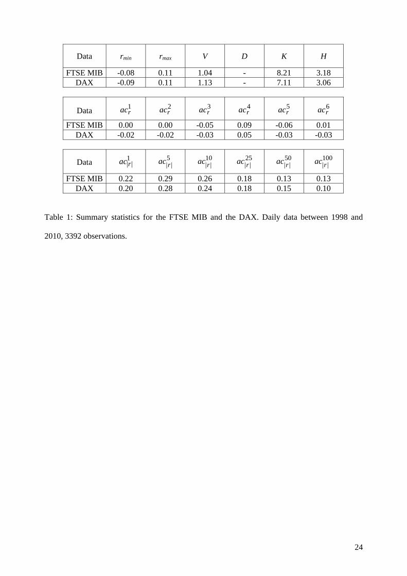
With the first two statistics, rmin and rmax, we look at the most negative and the most
positive daily log price change, respectively. As reported in Table 1, both the FTSE MIB and the
DAX produced extreme returns of around ±10 percent between 1998 and 2010. In comparison,
the extreme returns of our model seem to be somewhat lower on average. For instance, the
median negative and positive extreme returns are given b 6 percent and 5 percent, respectively. 2 Our model is related to that of Westerhoff and Franke (2011). Technically, their approach consists of only our
inner regime. On the one hand, this makes their model simpler than ours. On the other hand, they have to fine-tune
their parameters very carefully. To generate bubble dynamics, but to prevent complete price explosions at the same
time, they have to set their average slope parameter to slightly below one. Our model is more robust in the sense
that it works for a somewhat larger parameter space. For instance, we can allow for a more unstable inner regime
when the outer regimes guarantee an eventual end of bubbles.
18
However, at least 5 percent of the simulation runs produce extreme returns larger than ±10
percent.
We obtain a similar result when we look at volatility estimates. For this reason, we
introduce the volatility estimator ∑ −−= ||)/1( 1tt PPTV , measuring the average absolute
return (T is the sample length, given here by T=3391 observations). The median volatility
estimate we obtain for our model is approximately 0.75 percent. For the Italian and German
stock markets, we find volatility estimates of around 1 percent. Given this evidence, we may
conclude that our model is able to produce excess volatility, and that its volatility is roughly
comparable to what we observe in actual stock markets (taking into account that the period 1998
to 2010 was, presumably, more volatile than the long-run average).
To capture the phenomenon of bubbles and crashes, we use the
statistic, which measures the average absolute distance between log prices and log fundamentals.
Apparently, this statistic is an indicator of the distortion in the market and quantifies, at least
partially, the size of bubbles and crashes. Unfortunately, this statistic cannot be computed for
actual markets, at least not as long as there is a reliable indicator of the markets’ fundamental
values. For our model, however, we find that 90 percent of the simulation runs have a distortion
between 8 and 15.5 percent. Hence, bubbles and crashes seem to be present in almost all
simulation runs.
∑ −= ||)/1( tt FPTD
***** Table 1 and 2 about here *****
Estimates for the kurtosis K are given by 8.21 for the Italian and 7.11 for the German
return distribution. The median value we obtain for our model is 5.38, which is close to these
values. Moreover, 95 percent of our simulation runs have a kurtosis of 4.3 or more. Since the
kurtosis of a normal distribution is given by 3, this can be regarded as a safe indicator of excess
kurtosis. A better indicator of the fat-tailedness of a return distribution is the Hill tail index H,
which we compute on the basis of the largest 5 percent of the absolute returns. For actual
markets, this statistic tends to hover between 3 and 4 and, indeed, for the Italian and German
19
stock markets they are given by 3.18 (FTSE MIB) and 3.06 (DAX). Our model comes quite
close to these figures. As we can see, 70 percent of the simulation runs yield Hill estimates
between 2.93 and 4.11. In other words, there is ample evidence that our model is able to
generate fat-tailed return distributions.
A further important stylized fact of financial markets concerns their unpredictability.
Table 1 presents the autocorrelation coefficients of the returns for the first six lags. These
autocorrelation coefficients are quite small, and imply that neither the Italian nor the German
stock market can be predicted, at least not based on past returns and linear methods. This
important feature is matched by our model quite nicely. The autocorrelation coefficients of the
simulated returns are essentially insignificant.
Finally, we turn to the markets’ tendency to produce volatility clustering and long
memory effects, two other closely related universal features of financial markets. The
predictability of the volatility can be detected via the autocorrelation coefficients of the absolute
returns (which we compute for lags 1, 5, 10, 25, 50 and 100). In real markets, these
autocorrelation coefficients are highly significant and decay slowly. Again, this also is the case
for the Italian and German markets, and for our artificial market.
It goes without saying that our model is not perfect. However, given the simplicity of our
setup, it is surprising to see how closely the data generated by our model comes to actual data.
Overall, our model has at least a certain ability to generate bubbles and crashes, excess
volatility, fat tails for the distribution of returns, uncorrelated returns and volatility clustering
and long memory effects – which are frequently regarded as the most important stylized facts of
financial markets.
5 Conclusions
We propose a simple financial market model with heterogeneous interacting speculators. Some
speculators believe in the persistence of bull and bear markets and thus optimistically buy if
20
prices are high and pessimistically sell if prices are low. Other speculators do the contrary, and
bet on mean reversion: they buy if markets are undervalued and sell if they are overvalued.
While some speculators are always active, other speculators only enter the market if prices are at
least a certain distance away from fundamentals. Apart form this (rather natural) assumption,
speculators follow piecewise-linear trading rules. Since the dynamics of our model is driven by
a discontinuous piecewise-linear map, it is possible to provide a more or less complete analytical
study of the model. The main contribution of this paper is to show that a stochastic version of
our model – in which we assume that speculators may randomly deviate from their core trading
principles – is able to generate quite realistic dynamics. Responsible for this outcome is the fact
that the dynamics result from a mixture of different dynamic regimes, including fixed point
dynamics, (quasi-)periodic dynamics, chaotic dynamics and divergent dynamics.
Our model may be extended in several directions, three of which are mentioned here. (1)
Recall that type 2 chartists and type 2 fundamentalists share the same market entry levels.
Relaxing this assumption would lead to a discontinuous piecewise-linear map with five
branches, and it would seem worthwhile to invest effort in exploring this more complicated
scenario. (2) One assumption of our stochastic model is that all six model parameters change
randomly at each time step. A natural question is whether realistic dynamics can also be
obtained if there are less frequent parameter changes. For instance, parameters may change only
from time to time, either randomly or due to social and/or economic considerations. (3) The
shape of our model is extremely flexible. It might therefore be possible to find quite alternative
parameter settings which also deliver reasonable dynamics. The question would then be a matter
of establishing which parameter setting is the most successful. We hope that Laura Gardini will
help us – again – to tackle some of these exciting issues.
21
References
Brock, W. and Hommes, C. (1998): Heterogeneous beliefs and routes to chaos in a simple asset
pricing model. Journal of Economic Dynamics Control, 22, 1235-1274.
Chiarella, C., Dieci, R. and Gardini, L. (2002): Speculative behaviour and complex asset price
dynamics: A global analysis. Journal of Economic Behavior and Organization, 49, 173-197.
Chiarella, C., Dieci, R. and He, X.-Z. (2009): Heterogeneity, market mechanisms, and asset
price dynamics. In: Hens, T. and Schenk-Hoppé, K.R. (eds.): Handbook of Financial
Markets: Dynamics and Evolution. North-Holland, Amsterdam, 277-344.
Cont, R. (2001): Empirical properties of asset returns: stylized facts and statistical issues.
Quantitative Finance, 1, 223-236.
Day, R. and Huang, W. (1990): Bulls, bears and market sheep. Journal of Economic Behavior
and Organization, 14, 299-329.
De Grauwe, P., Dewachter, H. and Embrechts, M. (1993): Exchange rate theory – chaotic
models of foreign exchange markets. Blackwell, Oxford.
Gaunersdorfer, A. and Hommes, C. (2007): A nonlinear structural model for volatility
clustering. In: G. Teyssière and A.P. Kirman (eds): Long Memory in Economics, Springer,
Berlin, 265-288.
He, X.-Z. and Li, Y. (2007): Power-law behaviour, heterogeneity, and trend chasing. Journal of
Economic Dynamics and Control, 31, 3396-3426.
Hommes, C. and Wagener, F. (2009): Complex evolutionary systems in behavioral finance. In:
Hens, T. and Schenk-Hoppé, K.R. (eds.): Handbook of Financial Markets: Dynamics and
Evolution. North-Holland, Amsterdam, 217-276.
Hommes, C. (2011): The heterogeneous expectations hypothesis: Some evidence from the lab.
Journal of Economic Dynamics and Control, 35, 1-24.
Huang, W. and Day, R. (1993): Chaotically switching bear and bull markets: the derivation of
stock price distributions from behavioral rules. In: Day, R. and Chen, P. (eds): Nonlinear
dynamics and evolutionary economics. Oxford University Press, Oxford, 169-182.
Huang,W., Zheng, H. and Chia, W.M., (2010): Financial crisis and interacting heterogeneous
agents. Journal of Economic Dynamics and Control, 34, 1105-1122.
Kirman, A. (1991): Epidemics of opinion and speculative bubbles in financial markets. In:
Taylor, M. (ed.): Money and Financial Markets. Blackwell: Oxford, 354-368.
Lux, T. (1995): Herd behaviour, bubbles and crashes. Economic Journal, 105, 881-896.
Lux, T. and Marchesi, M., (1999): Scaling and criticality in a stochastic multi-agent model of a
financial market. Nature, 397, 498-500.
22
Lux, T. and Ausloos, M. (2002): Market fluctuations I: Scaling, multiscaling, and their possible
origins. In: Bunde, A., Kropp, J. and Schellnhuber, H. (eds.): Science of disaster: climate
disruptions, heart attacks, and market crashes. Springer: Berlin, 373-410.
Lux, T. (2009): Stochastic behavioural asset-pricing models and the stylize facts. In: Hens, T.
and Schenk-Hoppé, K.R. (eds.): Handbook of Financial Markets: Dynamics and Evolution.
North-Holland, Amsterdam, 161-216.
Mantegna, R. and Stanley, E. (2000): An introduction to econophysics. Cambridge University
Press: Cambridge.
Menkhoff, L. and Taylor, M. (2007): The obstinate passion of foreign exchange professionals:
technical analysis. Journal of Economic Literature, 45, 936-972.
Tramontana, F., Westerhoff, F. and Gardini, L. (2010): On the complicated price dynamics of a
simple one-dimensional discontinuous financial market model with heterogeneous interacting
traders. Journal of Economic Behavior and Organization, 74, 187-205.
Tramontana, F., Westerhoff, F. and Gardini, L., (2011a): A simple financial market model with
chartists and fundamentalists: market entry levels and discontinuities. Working Paper.
Tramontana, F., Gardini, L. and Westerhoff, F. (2011b): Intricate asset price dynamics and one-
dimensional discontinuous maps. In: Puu, T. and Panchuck, A. (eds): Advances in nonlinear
economic dynamics. Nova Science Publishers, in press.
Tramontana, F., Gardini, L. and Westerhoff, F. (2011c): Heterogeneous speculators and asset
price dynamics: further results from a one-dimensional discontinuous piecewise-linear map.
Computational dynamics, in press.
Tramontana, F., Gardini, L. and Westerhoff, F. (2011d): One-dimensional maps with two
discontinuity points and three linear branches: mathematical lessons for understanding the
dynamics of financial markets. Working Paper.
Tramontana, F., Gardini, L. and Westerhoff, F. (2012): The bull and bear market models of Day
and Huang: Some extensions and new results. Working Paper.
Westerhoff, F. (2004): Multiasset market dynamics. Macroeconomic Dynamics, 8, 596-616.
Westerhoff, F. and Dieci, R. (2006): The effectiveness of Keynes-Tobin transaction taxes when
heterogeneous agents can trade in different markets: a behavioral finance approach. Journal
of Economic Dynamics and Control, 30, 293-322.
Westerhoff, F. (2009): Exchange rate dynamics: A nonlinear survey. In: Rosser, J.B., Jr. (ed):
Handbook of Research on Complexity. Edward Elgar, Cheltenham, 287-325.
Westerhoff, F. and Franke, R. (2011): Converse trading strategies, intrinsic noise and the
stylized facts of financial markets. Quantitative Finance, in press.