One-dimensional Fermi accelerator model with moving wall described by anonlinear van der Pol oscillator
Tiago Botari1 and Edson D. Leonel1,2
1Departamento de Fısica–UNESP–Univ Estadual Paulista, Av. 24A 1515, 13506-900 Rio Claro, SP, Brazil2Abdus Salam ICTP, 34100 Trieste, Italy
(Received 18 June 2012; published 7 January 2013)
A modification of the one-dimensional Fermi accelerator model is considered in this work. The dynamics ofa classical particle of mass m, confined to bounce elastically between two rigid walls where one is described bya nonlinear van der Pol type oscillator while the other one is fixed, working as a reinjection mechanism of theparticle for a next collision, is carefully made by the use of a two-dimensional nonlinear mapping. Two cases areconsidered: (i) the situation where the particle has mass negligible as compared to the mass of the moving walland does not affect the motion of it; and (ii) the case where collisions of the particle do affect the movement of themoving wall. For case (i) the phase space is of mixed type leading us to observe a scaling of the average velocityas a function of the parameter (χ ) controlling the nonlinearity of the moving wall. For large χ , a diffusion on thevelocity is observed leading to the conclusion that Fermi acceleration is taking place. On the other hand, for case(ii), the motion of the moving wall is affected by collisions with the particle. However, due to the properties ofthe van der Pol oscillator, the moving wall relaxes again to a limit cycle. Such kind of motion absorbs part of theenergy of the particle leading to a suppression of the unlimited energy gain as observed in case (i). The phasespace shows a set of attractors of different periods whose basin of attraction has a complicated organization.
As first proposed by Enrico Fermi [1] as an attemptto describe the high energy of cosmic particles interactingwith moving magnetic clouds, the Fermi accelerator modelconsists of a classical particle of mass m (denoting the cosmicparticle) confined to bounce between two rigid walls. One isperiodically moving in time (in correspondence to the movingmagnetic clouds) while the other one is fixed (working asa returning mechanism for a next collision with the movingwall). The phase space of the model is defined by the typeof motion of the moving wall. For a smoothly periodicmotion—say, a sinusoidal function—periodic islands, chaoticseas, and a set of invariant Kolmogorov-Arnold-Moser (KAM)curves are all observed coexisting in the phase space. Thediffusion in the velocity is limited by the KAM curves and,deceptively, Fermi acceleration (unlimited energy growth) isnot present. On the other hand, when the motion of the movingwall is considered of sawtooth type, the mixed structureof the phase space is not observed anymore and unlimitedenergy is observed. The interest in Fermi acceleration hasthen increased and several applications have been observedin different areas of science including astrophysics [2,3],plasma physics [4], optics [5,6], atomic physics [7], andeven in time-dependent billiard problems [8]. The traditionalapproach to describe Fermi acceleration developing in suchtypes of time-dependent systems is generally given in terms ofa diffusion process which takes place in momentum space. Theevolution of the probability density function for the magnitudeof particle velocities as a function of the number of collisions isdetermined by the Fokker-Planck equation, and results for theone-dimensional case consider either static wall approxima-tion or moving boundary description [9–11]. The phenomenon,however, seems not to be robust since dissipation is assumedto be a mechanism to suppress Fermi acceleration [12].
In this paper we revisit the one-dimensional Fermi accel-erator model, however, considering the motion of the movingwall given by a van der Pol equation and considering two cases:(i) the mass of the particle is negligible as compared to the massof the moving wall; and (ii) the collisions of the particle affectthe motion of the moving wall, which are restored to a limitcycle after a relaxation time. Our main goal is to understandand describe the influences of a limit cycle type motion ofthe moving wall to the dynamics of the particle and henceto the properties of the average velocity in the phase space.The results of our approach considered in this model mayhave applications to a different set of systems, particularlyto the class of time-dependent billiard problems. Indeed thepresent system can be a corresponding classical prototype tomodel results involving applications in cavity optomechanics[13,14], mechanical [15,16], and nanomechanical resonators[17]. In such systems, the influence of a laser beam, whichimparts momentum to a mirror (wall), may lead also to atype of synchronization of either micromechanical [18] ornanomechanical resonators [19]. The model we are interestedin then consists of a classical particle of mass m which sufferscollisions with two walls. One is moving in time whosemotion is described by a van der Pol equation leading to alimit cycle dynamics while the other one is fixed and worksas a returning mechanism of the particle to a next collisionwith the moving wall. The dynamics is constructed by atwo-dimensional nonlinear mapping for the variables velocityof the particle and time. For case (i) the dynamics leadsto a mixed phase space structure where periodic islands areobserved surrounded by chaotic seas and limited by a set ofinvariant KAM curves. As soon as the parameter χ controllingthe nonlinearity of the moving wall rises, the position of thelowest invariant KAM curve rises too, leading to an increase inthe average velocity of the particle. Scaling arguments are usedto describe the behavior of the average velocity as a function
TIAGO BOTARI AND EDSON D. LEONEL PHYSICAL REVIEW E 87, 012904 (2013)
of the parameter χ and a set of critical exponents is obtained.On the other hand, for case (ii), the collisions of the particlewith the moving wall indeed affect the dynamics of such wall,leading it out of or into the limit cycle. After a relaxation time,however, the moving wall reaches the limit cycle again. A setof different periodic attractors is observed in the phase spaceand the organization of the basin of attraction of each attractorappears to be complicated. A histogram of periodic orbits isalso constructed leading us to observe a high incidence of lowperiod orbits as compared to large period orbits.
This paper is organized as follows. In Sec. II we constructthe model and describe the equations that give the dynamicsof the motion. Section III is devoted to discussing the caseof negligible mass of the particle including results of thephase space, characterization of chaotic orbits, and scalingof the average velocity. The case where collisions of theparticle affect the motion of the moving wall is describedin Sec. IV. Conclusions and final remarks are presentedin Sec. V.
II. THE MODEL AND THE MAPPING
In this section we present all the details needed for theconstruction of the mapping. The model consists of a classicalparticle of mass m which is confined to bounce betweentwo walls. One of them is assumed to be fixed at positionx = L and collisions are assumed to be elastic. The otherone moves in time and the oscillations are described by avan der Pol oscillator whose average position is x = 0. Wedescribe two situations where (i) the mass of the particle issufficiently small as compared to the mass of the movingwall and (ii) the case where the mass of the particle is notnegligible, therefore affecting the dynamics of the movingwall.
Indeed, the van der Pol oscillator is a generalization of aharmonic oscillator that contains a nonlinear and dissipativeterm. Applications of the van der Pol oscillator can befound in many different systems including dusty plasma[20,21], coupled oscillators [22,23], and many others. Thedifferential equation describing the van der Pol oscillator isdefined as
Md2x
dt2+ b(x2 − x0
2)dx
dt+ κx = F0 sin(ωf t), (1)
where M is the mass, b denotes the dissipative term, and κ
is the Hook constant. The nonlinear term (x2 − x02) creates
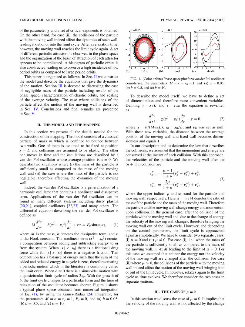
a competition between adding and subtracting energy to orfrom the system. When |x| < |x0| there is a frictional dragforce while for |x| > |x0| there is a negative friction. Thiscompetition has a balance of energy such that the sum of theadded and reduced energy in a cycle is zero, therefore creatinga periodic motion which in the literature is commonly calledthe limit cycle. When b ≈ 0 there is a sinusoidal motion witha quasicircular limit cycle of radius 2x0. With the growth ofb, the limit cycle changes to a particular form and the time ofrelaxation of the oscillator becomes shorter. Figure 1 showsa typical phase space obtained from numerical integrationof Eq. (1), by using the Gauss-Radau [24] integrator, forthe parameters M = κ = x0 = 1, F0 = 0, and (a) b = 0.05,(b) b = 0.5, and (c) b = 10.
FIG. 1. (Color online) Phase space plot for a van der Pol oscillatorconsidering the parameters M = κ = x0 = 1 and (a) b = 0.05,(b) b = 0.5, and (c) b = 10.
To describe the model itself, we have to define a setof dimensionless and therefore more convenient variables.Defining y = x/L and τ = tω0 the equation is rewrittenas
d2y
dτ 2+ χ (y2 − y0
2)dy
dτ+ y = 0, (2)
where χ = b/(Mω0L), y0 = x0/L, and F0 was set as null.With these new variables, the distance between the averageposition of the moving wall and fixed wall becomes dimen-sionless and equals 1.
In our description and to determine the law that describesthe collisions, we assumed that the momentum and energy areconserved at the instant of each collision. With this approach,the velocities of the particle and the moving wall after the(n + 1)th collision are
vp
n+1 = μ − 1
1 + μ
(vp
n − vwn
) + vwn ,
(3)
vwn+1 = 2μ
1 + μ
(vp
n − vwn
) + vwn ,
where the upper indices p and w stand for the particle andmoving wall, respectively. Here μ = m/M denotes the ratio ofmass of the particle and the mass of the moving wall. Thereforethe particle and the moving wall change energy and momentumupon collision. In the general case, after the collision of theparticle with the moving wall and, due to the change of energy,the velocity of the moving wall changes, therefore bringing themoving wall out of the limit cycle. However, and dependingon the control parameters, the limit cycle is approachedagain asymptotically. We have to consider two separate cases:(i) μ = 0 and (ii) μ �= 0. For case (i), i.e., when the mass ofthe particle is sufficiently small as compared to the mass ofthe moving wall, m � M leading to the limit of μ = 0. Forthis case we assumed that neither the energy nor the velocityof the moving wall are changed after the collision. For case(ii) where μ > 0, the collisions of the particle with the movingwall indeed affect the motion of the moving wall bringing it inor out of the limit cycle. It, however, relaxes again to the limitcycle as time evolves. We therefore consider the two cases inseparate sections.
III. THE CASE OF μ = 0
In this section we discuss the case of μ = 0. It implies thatthe velocity of the moving wall is not affected by the change
012904-2
ONE-DIMENSIONAL FERMI ACCELERATOR MODEL WITH . . . PHYSICAL REVIEW E 87, 012904 (2013)
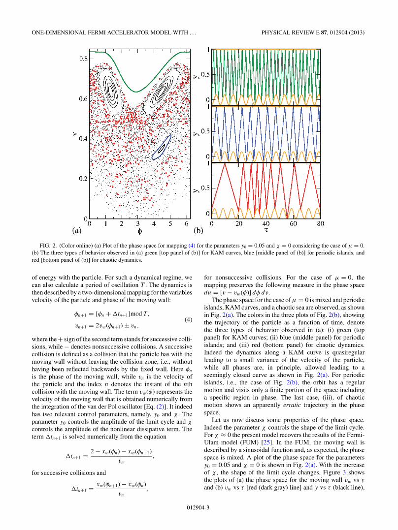
FIG. 2. (Color online) (a) Plot of the phase space for mapping (4) for the parameters y0 = 0.05 and χ = 0 considering the case of μ = 0.(b) The three types of behavior observed in (a) green [top panel of (b)] for KAM curves, blue [middle panel of (b)] for periodic islands, andred [bottom panel of (b)] for chaotic dynamics.
of energy with the particle. For such a dynamical regime, wecan also calculate a period of oscillation T . The dynamics isthen described by a two-dimensional mapping for the variablesvelocity of the particle and phase of the moving wall:
φn+1 = [φn + �tn+1]mod T ,(4)
vn+1 = 2vw(φn+1) ± vn,
where the + sign of the second term stands for successive colli-sions, while − denotes nonsuccessive collisions. A successivecollision is defined as a collision that the particle has with themoving wall without leaving the collision zone, i.e., withouthaving been reflected backwards by the fixed wall. Here φn
is the phase of the moving wall, while vn is the velocity ofthe particle and the index n denotes the instant of the nthcollision with the moving wall. The term vw(φ) represents thevelocity of the moving wall that is obtained numerically fromthe integration of the van der Pol oscillator [Eq. (2)]. It indeedhas two relevant control parameters, namely, y0 and χ . Theparameter y0 controls the amplitude of the limit cycle and χ
controls the amplitude of the nonlinear dissipative term. Theterm �tn+1 is solved numerically from the equation
�tn+1 = 2 − xw(φn) − xw(φn+1)
vn
,
for successive collisions and
�tn+1 = xw(φn+1) − xw(φn)
vn
,
for nonsuccessive collisions. For the case of μ = 0, themapping preserves the following measure in the phase spacedu = [v − vw(φ)] dφ dv.
The phase space for the case of μ = 0 is mixed and periodicislands, KAM curves, and a chaotic sea are observed, as shownin Fig. 2(a). The colors in the three plots of Fig. 2(b), showingthe trajectory of the particle as a function of time, denotethe three types of behavior observed in (a): (i) green (toppanel) for KAM curves; (ii) blue (middle panel) for periodicislands; and (iii) red (bottom panel) for chaotic dynamics.Indeed the dynamics along a KAM curve is quasiregularleading to a small variance of the velocity of the particle,while all phases are, in principle, allowed leading to aseemingly closed curve as shown in Fig. 2(a). For periodicislands, i.e., the case of Fig. 2(b), the orbit has a regularmotion and visits only a finite portion of the space includinga specific region in phase. The last case, (iii), of chaoticmotion shows an apparently erratic trajectory in the phasespace.
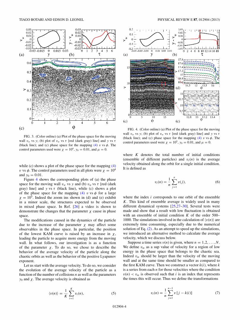
Let us now discuss some properties of the phase space.Indeed the parameter χ controls the shape of the limit cycle.For χ ≈ 0 the present model recovers the results of the Fermi-Ulam model (FUM) [25]. In the FUM, the moving wall isdescribed by a sinusoidal function and, as expected, the phasespace is mixed. A plot of the phase space for the parametersy0 = 0.05 and χ = 0 is shown in Fig. 2(a). With the increaseof χ , the shape of the limit cycle changes. Figure 3 showsthe plots of (a) the phase space for the moving wall vw vs y
and (b) vw vs τ [red (dark gray) line] and y vs τ (black line),
012904-3
TIAGO BOTARI AND EDSON D. LEONEL PHYSICAL REVIEW E 87, 012904 (2013)
FIG. 3. (Color online) (a) Plot of the phase space for the movingwall vw vs y; (b) plot of vw vs τ [red (dark gray) line] and y vs τ
(black line); and (c) phase space for the mapping (4) v vs φ. Thecontrol parameters used were χ = 104, y0 = 0.01, and μ = 0.
while (c) shows a plot of the phase space for the mapping (4)v vs φ. The control parameters used in all plots were χ = 104
and y0 = 0.01.Figure 4 shows the corresponding plots of (a) the phase
space for the moving wall vw vs y and (b) vw vs τ [red (darkgray) line] and y vs τ (black line), while (c) shows a plotof the phase space for the mapping (4) v vs φ for a largeχ = 105. Indeed the zoom ins shown in (d) and (e) exhibitin a minor scale, the structures expected to be observedin mixed phase space. In Ref. [26] a video is shown todemonstrate the changes that the parameter χ cause in phasespace.
The modifications caused in the dynamics of the particledue to the increase of the parameter χ may affect someobservables in the phase space. In particular, the positionof the lowest KAM curve is raised by an increase in χ ,leading the particle to acquire more energy from the movingwall. In what follows, our investigation is as a functionof the parameter χ . To do so, we chose to describe thebehavior of the average velocity of the particle along thechaotic orbits as well as the behavior of the positive Lyapunovexponent.
Let us start with the average velocity. To do so, we considerthe evolution of the average velocity of the particle as afunction of the number of collisions n as well as the parametersy0 and χ . The average velocity is obtained as
〈v(n)〉 = 1
K
K∑
i=1
vi(n), (5)
FIG. 4. (Color online) (a) Plot of the phase space for the movingwall vw vs y; (b) plot of vw vs τ [red (dark gray) line] and y vs τ
(black line); and (c) phase space for the mapping (4) v vs φ. Thecontrol parameters used were χ = 105, y0 = 0.01, and μ = 0.
where K denotes the total number of initial conditions(ensemble of different particles) and vi(n) is the averagevelocity obtained along the orbit for a single initial condition.It is defined as
vi(n) = 1
n
n∑
j=1
v(j ), (6)
where the index i corresponds to one orbit of the ensembleK . This kind of ensemble average is widely used in manydifferent dynamical systems [25,27–30]. Several tests weremade and show that a result with low fluctuation is obtainedwith an ensemble of initial condition K of the order 500–1000. The simulations involved in the calculation of 〈v(n)〉 areextremely time consuming, especially due to the numericalsolution of Eq. (2). As an attempt to speed up the simulations,we introduced an alternative method to calculate the averagevelocity, which we discuss below.
Suppose a time series v(n) is given, where n = 1,2, . . . ,N .We define vm as a sup value of velocity for a region of lowenergy in the phase space that belongs to the chaotic sea.Indeed vm should be larger than the velocity of the movingwall and at the same time should be smaller as compared tothe first KAM curve. Then we construct a vector k(i), where k
is a series from each n for those velocities where the conditionv(n) < vm is observed such that i is an index that representsthe times this will occur. Thus we define the transformations
vi(n) = 1
n
n−1∑
j=1
v [j − k(i)] (7)
012904-4
ONE-DIMENSIONAL FERMI ACCELERATOR MODEL WITH . . . PHYSICAL REVIEW E 87, 012904 (2013)
100 102 104 106 108
n10-4
10-3
10-2
10-1
<v>
y0=1x10⁻³ χ = 1x10⁴ (normal)
y0=1x10⁻³ χ = 1x10⁴
y0=1x10⁻³ χ = 1x10⁶ (normal)
y0=1x10⁻³ χ = 1x10⁶
y0=1x10⁻⁴ χ = 1x10⁷ (normal)
y0=1x10⁻⁴ χ = 1x10⁷
y0=1x10⁻⁴ χ = 1x10⁸ (normal)
y0=1x10⁻⁴ χ = 1x10⁸
FIG. 5. (Color online) Plot of 〈v〉 vs n for different controlparameters and initial conditions, as labeled in the figure. Bulletsdenote the traditional (normal) method of evolving an ensem-ble of initial conditions and squares correspond to the proposedmethod.
and
〈v〉 (n) = limN→∞
1
K ′
K ′∑
i=1
vi(n), (8)
where K ′ = dim(k), and dim denotes the dimension of vectork. Using this procedure, the evolution of a single orbit followedfor a long time is enough to obtain the average propertiesand therefore to speed up the simulations as compared tothe normal method of evolving a long ensemble of differentinitial conditions. To have an idea of the accuracy of theproposed method, Fig. 5 shows a plot of 〈v〉 vs n for differentcontrol parameters and initial conditions, as labeled in thefigure. Bullets correspond to the traditional (normal) method ofevolving an ensemble of initial conditions [25], while squaresdenote the proposed method. We see that curves generated bythe two methods remarkably overlap each other, confirmingthe procedure can be used. Of course some precautionswere taken as, for example, when the particle is trapped ina sticky region. In this case the problem is fixed by justincreasing the number of collisions or by a change in the initialcondition.
Having established the procedure to obtain the averagevelocity, let us now discuss some properties as a functionof the control parameters. Indeed, starting with an initialcondition with low velocity, the average velocity 〈v〉 growsfor small values of n and, after passing by a crossover regime,it becomes constant for large enough n. The changeover fromgrowth to the regime marked by a constant plateau defines afinal average velocity 〈v〉f . Figure 6 shows different plots of〈v〉 vs n for the parameter y0 = 0.001 and different values ofχ , as labeled in the figure. For χ ≈ 0, the results obtainedrecover those already known for the traditional FUM [25]. Asshown in Fig. 6, a change in χ leads the asymptotic dynamicsfor large n to reach a different saturation of the velocity. Itis expected that a similar behavior is to be observed as theparameter y0 varies, and it indeed happens. A plot of the final
100 101 102 103 104 105 106 107 108
n10-3
10-2
10-1
100
<v>
1x10⁴
1x10⁵
3x10⁵
1x10⁶
2x10⁶
3x10⁶
5x10⁶
χ
FIG. 6. (Color online) Plot of the average velocity as a functionof n for the parameters y0 = 0.001, μ = 0 and different values of χ ,as labeled in the figure.
average velocity 〈v〉f as a function of the parameter y0 isshown in Fig. 7(a). The behavior of the final average velocityas a function of χ is shown in Fig. 8 for different values of
FIG. 7. (Color online) (a) Plot of 〈v〉FUf vs y0. A fitting furnishes
an exponent α = 0.52(2). (b) Plot of χc vs y0. A numerical fit givesan exponent z = −2.1(2). (c) Overlap of different curves of 〈v〉 ontoa single plot, after a suitable rescale of the axis, for different controlparameters, as labeled in the figure and μ = 0.
012904-5
TIAGO BOTARI AND EDSON D. LEONEL PHYSICAL REVIEW E 87, 012904 (2013)
FIG. 8. (Color online) Plot of the final average velocity as afunction of χ for different values of y0, as labeled in the figure andconsidering μ = 0.
y0, as labeled in the figure. We see from this figure that thefinal average velocity stays in a plateau for a large range ofχ and that it depends on y0. After a critical parameter χc isreached, the average velocity starts to increase with a powerlaw. Based on the behavior observed in Fig. 8, we propose thefollowing:
(1) For χ � χc, the average velocity 〈v〉f behaves as
〈v〉f (χ ) ∝ yα0 , (9)
where α is a critical exponent;(2) For χ � χc, the average velocity is written as
〈v〉f (χ ) ∝ χβ, (10)
where β is also a critical exponent.(3) Finally, the crossover χc that marks the change from the
plateau to the regime of growth is given by
χc ∝ yz0, (11)
where z is called a dynamical exponent.After considering these three initial suppositions, the
description of the asymptotic average velocity 〈v〉f may bemade in terms of a scaling function of the type
〈v〉f (χ,y0) = l 〈v〉f (lAχ,lBy0), (12)
where l is the scaling factor and A and B are scaling exponents.If we choose properly the scaling factor l, it is possible to relatethe scaling exponents A and B with the critical exponentsα, β, and z. Choosing lAχ = 1, which leads to l = χ−1/A,Eq. (12) is rewritten as
〈v〉f (χ,y0) = χ−1/A 〈v〉f (1,χ−B/Ay0). (13)
Comparing Eqs. (10) and (13), we obtain β = −1/A.Choosing now lBy0 = 1, we have l = y
−1/B
0 and Eq. (12)is written as
〈v〉f (χ,y0) = y−1/B
0 〈v〉f(y
−A/B
0 χ,1). (14)
An immediate comparison of Eqs. (9) and (14) gives us α =−1/B. Given the two different expressions of the scaling factorl, it is easy to obtain a relation for the dynamical exponent z,that is given by
z = α
β. (15)
The critical exponents α, β, and z can be obtained via extensivenumerical simulations. For the initial regime of plateau forχ � χc, a power law fitting to the plot of 〈v〉pf vs y0 givesα = 0.52(1). On the other hand, the regime of growth for thecurves of 〈v〉f vs χ , i.e., for χ � χc, we obtain β = 1.2(3).Finally, a fitting to the plot of χc vs y0 gives z = −2.1(1).Figures 7(a) and 7(b) show the behavior of 〈v〉FU
f vs y0 andχc vs y0, respectively.
Given that the critical exponents are now obtained, asuitable rescale of the axis from the plot shown in Fig. 8can be made to overlap all curves of 〈v〉f onto a singleand seemingly universal plot, as shown in Fig. 7(c). Thisoverlap confirms the behavior of the average velocity at theasymptotic dynamics is scaling invariant with respect to bothy0 and χ .
Given we have described the behavior of the averagevelocity, let us now discuss the Lyapunov exponent forchaotic orbits. Indeed, the Lyapunov exponent gives theexponential rate of divergence or convergence of the evolutionof close initial conditions in phase space. Thus when atleast one Lyapunov exponent λ is positive, the system hasa chaotic component. The Lyapunov exponent is definedas [31]
λi = limn→∞
1
nln |�i |, i = 1,2, (16)
where �i denote the eigenvalues of matrix M = ∏nj=1 Jj ,
where Jj is the Jacobian matrix evaluated along the orbit(vj ,φj ).
For the model described by the mapping (4) and consideringa fixed value of y0, the positive Lyapunov exponent averagedalong the chaotic sea in the regime of low energy decreases asthe control parameter χ increases. Figure 9 shows the behaviorof the Lyapunov exponent as a function of the number ofcollisions with the moving wall for the parameter y0 = 0.01,μ = 0 and (a) χ = 5 × 10² and χ = 1 × 10³; (b) χ = 5 × 10³
and χ = 1 × 10⁴; and (c) χ = 5 × 10⁴ and χ = 1 × 105.A possible explanation of the decrease of the Lyapunov
exponent as an increase of χ is due to the shape of thelimit cycle. Indeed, for sufficiently small χ , the shape ofthe limit cycle looks more like a sine function. However, asthe parameter χ increases, the shape describing the motion ofthe moving wall has parts of large regularity: those where itmoves slowly, and parts where it moves very fast. Therefore,we expected that, as the parameter χ increases, the particlesuffers more collisions with the regular motion of the movingwall. Eventually it collides with a region where the movingwall is moving very fast, therefore leading to a large exchangeof energy, producing the regimes of growing velocities, asdiscussed before. Figure 10 shows plots of different trajectoriesof the particle as a function of time. The vertical axiscorresponds to the position, while horizontal axis denotes thetime. The parameters used were y0 = 10−2, μ = 0 and (a)
012904-6
ONE-DIMENSIONAL FERMI ACCELERATOR MODEL WITH . . . PHYSICAL REVIEW E 87, 012904 (2013)
0 2×10⁷
4×10⁷
6×10⁷
8×10⁷
1×10⁸
n0.4
0.45
0.5
0.55
0.6
0.65
λ
χ = 5x10² <λ> = 0.544(2)
χ = 1x10³ <λ> = 0.530(3)
0 2×10⁷
4×10⁷
6×10⁷
8×10⁷
1×10⁸
n0.2
0.25
0.3
0.35
0.4
0.45
λ
χ= 5x10³ <λ> = 0.34(1)
χ= 1x10⁴ <λ> = 0.36(1)
0 2×10⁷
4×10⁷
6×10⁷
8×10⁷
1×10⁸
n
-0.05
0
0.05
0.1
0.15
λ
χ = 5x10⁴ <λ> = 0.041(1)
χ = 1x10⁵ <λ> = 0.016(2)
y0
= 10-2
(a)
(c)
(b)
FIG. 9. (Color online) Plot of the Lyapunov exponent averagedover the chaotic sea for mapping (4) considering the control parametery0 = 0.01 and (a) χ = 5 × 10² and χ = 1 × 10³; (b) χ = 5 × 10³
and χ = 1 × 10⁴; and (c) χ = 5 × 10⁴ and χ = 1 × 10⁵.
and (c) χ = 102; and (b) and (d) χ = 105. Figures 10(a) and10(c) describe the case of χ � χc, leading to a motion of themoving wall to be described almost like a sinusoidal function.We see that the trajectories depart from each other very quickly(after a few collisions), as shown in Fig. 10(c), just after a fewcollisions. The initial velocity used in Figs. 10(a) and 10(c)was V0 = 0.02 and considering the initial phase as φ0 = 4.27for the orange (dotted), φ0 = 5.94 for the green (dashed), andφ0 = 0.72 for the blue (line) curves. For Figs. 10(b) and 10(d),the initial velocity is V0 = 0.02, while the initial phases areφ0 = 0.58 for the trajectory in orange (dotted), φ0 = 1.00,
for that in green (dashed), and φ0 = 3.82, for that in blue(line). One can see clearer that in Figs. 10(a) and 10(c),the separation of neighboring particles happens quickly, ascompared to Figs. 10(b) and 10(d).
IV. THE CASE OF μ �= 0
Let us consider in this section the case of μ �= 0. When theparticle collides with the moving wall, it perturbs the motionof the moving wall, bringing it into or out of the limit cycle. Asthe time evolves, the oscillator pushes the dynamics back to thelimit cycle, restoring the dynamics. Under this circumstance,the mapping is now written as
vp
n+1 = μ − 1
1 + μ
(vp
n − vwn
) + vwn ,
vwn+1 = 2μ
1 + μ
(vp
n − vwn
) + vwn ,
tn+1 = tn + �tn+1, yn+1 = yw(φn+1),
where vp is the velocity of the particle, vw is the velocity ofthe moving wall, μ is the ratio of mass of the particle and massof the wall, t is the time, y is the position of the particle, andyw is the position of the moving wall upon collision. The term�tn+1 is obtained in the same way as made for the case ofμ = 0 with a numerical accuracy of 10−12.
FIG. 10. (Color online) Plot of three trajectories of the particleas a function of time. The initial velocity used in (a) and (c) wasV0 = 0.02 and different initial phases as φ0 = 4.27 for the orange(dotted), φ0 = 5.94 for the green (dashed), and φ0 = 0.72 for theblue (line) curves. For (b) and (d), the initial velocity is V0 = 0.02,while the initial phases are φ0 = 0.58 for the trajectory in orange(dotted), φ0 = 1.00 for that in green (dashed), and φ0 = 3.82 forthat in blue (line). The parameters used were y0 = 10−2, μ = 0, and(a) and (c) χ = 102 and (b) and (d) χ = 105.
The phase space is now defined by (y,v,vw), i.e., theposition of the moving wall at the instant of the collision y,the velocity of the particle v, and the velocity of the movingwall vw. Depending on the initial conditions and on the setof control parameters, the dynamics evolves to different fixedpoints, after passing by a transient. Therefore, we investigatethe basin of attraction for the fixed points considering the
FIG. 11. (Color online) Plot of the phase space v vs x. Squarerepresents different attractors, yellow denotes the initial transient.(b) Phase space for the van der Pol oscillator when it is perturbed bycollisions with the particle. Squares denote the instant of collision.The parameters used are y0 = 10−3, μ = 0.004, and χ = 106.
012904-7
TIAGO BOTARI AND EDSON D. LEONEL PHYSICAL REVIEW E 87, 012904 (2013)
FIG. 12. (Color online) (a) Basin of attraction v0 vs φ0. (b) Fixedpoints v vs x. The parameters used are y0 = 10−3, μ = 0.004, andχ = 106.
parameters χ = 106, y0 = 0.001, and μ = 0.004. The ellipticfixed points observed in the case μ = 0, become sinks aftera bifurcation and initial conditions close enough converge tothem asymptotically, as shown in Fig. 11.
To construct a basin of attraction we set the initial conditionswith the position of the moving wall along the limit cycle whichis obtained from the numerical solution of the integration ofthe van der Pol oscillator. Thus the initial condition evolvesin time until it reaches a regime of convergence to differentattractors. After analyzing the plots of the basin of attraction,we can identify several attractors with different periods, asshown in Fig. 12.
Considering v0 > 0.25 we found only attractors of period1. We can compare the basin of attraction with the phasespace in the case of μ = 0 and note several similarities as,for example, regions of periodic islands become regions thatlead the dynamics to a periodic attractor, as shown in Fig. 13.The parameters used to construct Fig. 13 were (a) y0 = 10−3,
FIG. 13. (Color online) (a) Basin of attraction v0 vs φ0 for theparameters y0 = 10−3, μ = 0.004, and χ = 106. (b) Phase space plotv vs φ for the parameters y0 = 10−3, μ = 0.004, and χ = 0.
5 10 15 20 25 30 35 40 45 50 55 60Period
10-4
10-3
10-2
10-1
100
Fre
quen
cy
FIG. 14. (Color online) Plot of the histogram of frequency ofinitial conditions for the period of the attractor. The parameters usedare y0 = 10−3, μ = 0.004, and χ = 106.
μ = 0.004, and χ = 106 and (b) y0 = 10−3, μ = 0.004, andχ = 0. In Ref. [32] a video is used to demonstrate the dynamicsof the system.
We see from Figs. 12 and 13 that the basin of attractionfor periodic orbits exhibit a quite complicated organization.To have an estimation of how many initial conditions evolvedto period 1, or period 2 and so on, we constructed a histogramof frequency of initial conditions that has as a final state, aperiodic attractor of period one, or two, etc. We found thatabout 70% of all initial conditions considered converge tothe period 1 sink. The other periods from 2 to 6 stay around1% and 10% and some initial conditions lead to observation ofperiods 20 and 60, as shown in Fig. 14. The control parametersused in the figure were y0 = 10−3, μ = 0.004, and χ = 106.
V. CONCLUSION
We revisited and described the dynamics of a classicalparticle suffering elastic collisions with two walls. One is fixedand the other one is moving according to the solution of a vander Pol oscillator. The mapping describing the dynamics ofthe model was constructed considering the cases where (i)the particle has negligible mass as compared to the massof the moving wall: and (ii) the collisions of the particle affectthe dynamics of the moving wall. Due to the properties of thevan der Pol oscillator, after the collisions, the moving wallrelaxes again to the limit cycle. We proposed an alternativemethod to calculate the average velocity of the particle alongthe phase space and, using it, we investigated the behavior ofthe average velocity of the particle. Scaling arguments wereused to describe the behavior of the average velocity. Hencecritical exponents α = 0.52(1), β = 1.2(3), and z = −2.1(1)were used to overlap all curves of average velocity onto asingle and seemingly universal plot. Lyapunov exponents werealso discussed as a function of the control parameters. As theparameter controlling the dissipation—and therefore the shapeof the limit cycle—is raised, the derivative of the position ofthe moving wall with respect to time may vary very fast from
012904-8
ONE-DIMENSIONAL FERMI ACCELERATOR MODEL WITH . . . PHYSICAL REVIEW E 87, 012904 (2013)
specific regions. Such variation leads the particle to gain alarge amount of energy upon collision, leading us to observea growth of the velocity of the particle for large enough timesuggesting the Fermi acceleration is taking place.
For case (ii) in which the mass of the particle is takeninto account along with the collisions with the moving wall,the dynamics of the system changes and the system becomesdissipative leading to the appearance of attractors in thedynamics. Considering that such attractors are far away fromthe infinity in the velocity domain, Fermi acceleration issuppressed, as was expected [12]. The basins of attractionof some attractors were obtained.
As a perspective of the study of this model with such typeof perturbations, one may include a synchronization of theoscillator; the information interchange is performed by theparticle and this procedure may be used to control chaos.Another aspect of the model that can be studied is related tothe introduction of two noninteracting particles in the system;however, the exchange of information happens through theperturbation caused by them in the moving wall. To commenton a possible experiment to where this classical model canbe of interest, if one considers an optical cavity where a laser
beam is injected [the particle is an analog of the laser beam(see Ref. [19] for specific examples), due to radiation pressure,there could be a displacement of one (or both) reflectingmirrors until the equilibrium condition is reached. As the laserescapes from the cavity, it could be injected to a differentcavity, therefore leading it to present a similar displacement asfor the first one, causing a synchronization between them. Adirect application involving an optomechanical system formedby micromechanical dielectric membranes was recently dis-cussed in Ref. [33].
ACKNOWLEDGMENTS
T.B. thanks CAPES and FAPESP. E.D.L. kindly ac-knowledges the financial support from Brazilian agenciesCNPq, FAPESP, and FUNDUNESP. E.D.L. acknowledgesthe hospitality of the ICTP during his visit. T.B. alsothanks Vinicius Santana, Roberto Eugenio Lagos Monaco,and Tadashi Yokoyama for fruitful discussions. This researchwas supported by resources supplied by the Center forScientific Computing (NCC/GridUNESP) of the Sao PauloState University (UNESP).
[1] E. Fermi, Phys. Rev. 75, 1169 (1949).[2] A. Veltri and V. Carbone, Phys. Rev. Lett. 92, 143901 (2004).[3] K. Kobayakawa, Y. S. Honda, and T. Samura, Phys. Rev. D 66,
083004 (2002).[4] A. V. Milovanov and L. M. Zelenyi, Phys. Rev. E 64, 052101
(2001).[5] F. Saif, I. Bialynicki-Birula, M. Fortunato, and W. P. Schleich,
Phys. Rev. A 58, 4779 (1998).[6] A. Steane, P. Szriftgiser, P. Desbiolles, and J. Dalibard, Phys.
Rev. Lett. 74, 4972 (1995).[7] G. Lanzano et al., Phys. Rev. Lett. 83, 4518 (1999).[8] A. Loskutov and A. B. Ryabov, J. Stat. Phys. 108, 995 (2002).[9] A. K. Karlis, P. K. Papachristou, F. K. Diakonos, V. Constan-
toudis, and P. Schmelcher, Phys. Rev. Lett. 97, 194102 (2006).[10] A. K. Karlis, P. K. Papachristou, F. K. Diakonos, V. Constan-
toudis, and P. Schmelcher, Phys. Rev. E 76, 016214 (2007).[11] A. K. Karlis, F. K. Diakonos, and V. Constantoudis, Chaos 22,
026120 (2012).[12] E. D. Leonel, J. Phys. A 40, F1077 (2007).[13] T. J. Kippenberg and K. J. Vahala, Science 321, 172 (2008).[14] F. Marquardt and S. M. Girvin, Physics 2, 40 (2009).[15] A. Schliesser, O. Arcizet, R. Riviere, G. Anetsberger, and T. J.
Kippenberg, Nat. Phys. 5, 509 (2009).[16] R. Riviere, S. Deleglise, S. Weis, E. Gavartin, O. Arcizet,
A. Schliesser, and T. J. Kippenberg, Phys. Rev. A 83, 063835(2001).
[17] M. Bagheri, M. Poot, M. Li, W. P. H. Pernice, and H. X. Tang,Nat. Nanotechnol. 6, 726 (2011).
[18] M. Zhang, G. S. Wiederhecker, S. Manipatruni, A. Barnard,P. McEuen, and M. Lipson, Phys. Rev. Lett. 109, 233906 (2012).
[19] C. A. Holmes, C. P. Meaney, and G. J. Milburn, Phys. Rev. E85, 066203 (2012).
[20] K. O. Menzel, O. Arp, and A. Piel, Phys. Rev. Lett. 104, 235002(2010).
[21] K. O. Menzel, O. Arp, A. Piel, Phys. Rev. E 84, 016405(2011).
[22] A. Bahraminasab, F. Ghasemi, A. Stefanovska, P. V. E. McClin-tock, and H. Kantz, Phys. Rev. Lett. 100, 084101 (2008).
[23] P. Rosenau and A. Pikovsky, Phys. Rev. Lett. 94, 174102(2005).
[24] E. Everhart, in Dynamics of Comets: Their Origin and Evolution,edited by A. Carusi Carusi and G. B. Valsecchi (D. Reidel,Dordrecht, 1985).
[25] E. D. Leonel, P. V. E. McClintock, and J. K. L. da Silva, Phys.Rev. Lett. 93, 014101 (2004).
[26] See Supplemental Material at http://link.aps.org/supplemental/10.1103/PhysRevE.87.012904 for a video where the phase spaceof the model is constructed for the case of μ = 0 and differentcontrol parameters.
[27] F. Lenz, F. K. Diakonos, and P. Schmelcher, Phys. Rev. Lett.100, 014103 (2008).
[28] J. A. Mendez-Bermudez and R. Aguilar-Sanchez, Phys. Rev. E85, 056212 (2012).
[29] D. Wu and S. Zhu, Phys. Rev. E 85, 061101 (2012).[30] A. Loskutov, A. Ryabov, and E. D. Leonel, Physica A 389, 5408
(2010).[31] J. P. Eckmann and D. Ruelle, Rev. Mod. Phys. 57, 617 (1985).[32] See Supplemental Material at http://link.aps.org/supplemental/
10.1103/PhysRevE.87.012904 for a video where the phase spaceof the model is constructed for the case of μ �= 0 and differentcontrol parameters.
[33] J. D. Thompson, B. M. Zwickl, A. M. Jayich, Florian Marquardt,S. M. Girvin, and J. G. E. Harris, Nature (London) 452, 72(2008).