Online Association Rule Mining

Christian Hidber International Computer Science Institute, Berkeley

hidber@icsi.berkeley.edu

Abstract We present a novel algorithm to compute large itemsets online. The user is free to change the support threshold any time during the first scan of the transaction sequence. The algorithm maintains a superset of all large itemsets and for each itemset a shrinking, deterministic interval on its support. After at most 2 scans the algorithm terminates with the precise support for each large itemset. Typically our algorithm is by an order of magnitude more memory efficient than Apriori or DIC.

1 Introduction

Mining for association rules is a form of data mining introduced in [AIS93]. The prototypical example is based on a list of purchases in a store. An association rule for this list is a rule such as “85% of all customers who buy product A and B also buy product C and D” . Discovering such customer buying patterns is useful for customer segmentation, cross-marketing, catalog design and product placement.

We give a problem description which follows [BMUT97]. The support of an itemset (set of items) in a transaction sequence is the fraction of all transactions containing the itemset. An itemset is called large if its support is greater or equal to a user-specified support thresh- old, otherwise it is called small. An association rule is an expression X =+ Y where X and Y are disjoint itemsets. The support of this rule is the support of X U Y. The confidence of this rule is the fraction of all transactions containing X that also contain Y, i.e. the support of X U Y divided by the support of X. In the example above, the “85%” is the confidence of the rule {A, B} 3 {C, D}. For an association rule to hold, it must have a support > a user-specified support threshold and a confidence 2 a user-specified confidence

Permission to ,,,akc digital or hard topics of all or part of this work fo’ persona\ or classroom ,lse is granted without fee provided tlut copies are not mac\c or distributed br profit or commercial advantage and thai topics bear this notice and the 11111 citation WI the lirst PaS. T” Copy ot,,cr,vise, tn republish, to post on scrvcrs or to rcdistributc to lists. requires prior specific permissioll and/or a fee. S~GMOD ‘99 Philadelphia PA Copyright ACM 1999 I-581 13-084-8/99/05...$5°0

threshold. Existing algorithms proceed in 2 steps to compute association rules:

1. Find all large itemsets.

2. For each large itemset 2, find all subsets X, such that the confidence of X + Z\X is greater or equal to the confidence threshold.

We address the first step, since the second step can already be computed online, c.f. [AY97]. Existing large itemset computation algorithms have an offline or batch behaviour: given the user-specified support threshold, the transaction sequence is scanned and rescanned, often several times, and eventually all large itemsets are produced. However, the user does not know, in general, an appropriate support threshold in advance. An inappropriate choice yields, after a long wait, either too many or too few large itemsets, which often results in useless or misleading association rules.

Inspired by online aggregation, c.f. [He196, HHW97], our goal is to overcome these difficulties by bringing large itemset computation online. We consider an algorithm to be online if: 1) it gives continuous feedback, 2) it is user controllable during processing and 3) it yields a deterministic and accurate result. Random sampling algorithms produce results which hold with some probability < 1. Thus we do not view them as being online.

In order to bring large itemset computation online, we introduce a novel algorithm called Carma (Continuous Association Rule Mining Algorithm). The algorithm needs, at most, two scans of the transaction sequence to produce all large itemsets.

During the first scan, the algorithm continuously con- structs a lattice of all potentially large itemsets (large with respect to the scanned part of the transaction se- quence). For each set in the lattice, Carma provides a deterministic lower and upper bound for its support. We continuously display, e.g. after each transaction processed, the resulting association rules to the user along with bounds on each rule’s support and confi- dence. The user is free to adjust the support and con-

145

fidence thresholds at any time. Adjusting the support threshold may result in an increased threshold for which the algorithm guarantees to include all large itemsets in the lattice. If satislied with the rules and bounds pro- duced so far, the user can stop the rule mining early.

During the second scan, the algorithm determines the precise support of each set in the lattice and continuously removes all small itemsets.

Existing algorithms need to rescan the transaction sequence before any output is produced. Thus, they can not be used on a stream of transactions read from a network for example. In contrast, using Carma’s first- scan algorithm, we can continuously process a stream of transactions and generate the resulting association rules online, not requiring a rescan.

While not being faster in general, Carma outperforms Apriori and DIC on low support thresholds and is up to 60 times more memory efficient.

2 Overview

The paper is structured as follows: In Section 3, we put our algorithm in the context of related work. In Section 4, we give a sketch of Carma. It uses two distinct algorithms Phase1 and PhaseII for the first and second scan respectively. In Section 5 we describe Phase1 in detail. In Subsection 5.1 we introduce .support lattices and support sequences, the building blocks for the Phase1 algorithm presented in Subsection 5.2. We illustrate Phase1 on an example in Subsection 5.3. We discuss changing support thresholds in Subsection 5.4. After a short description of Phase11 in Subsection 6.1, we combine in Subsection 6.2 Phase1 with PhaseII, yielding Carma. In Section 7 we discuss our implementation. After a brief discussion of implementa,tional details in Subsection 7.1, we compare in Subsection 7.2 the performance of Carma with Apriori and DIC. In Subsection 7.3 we analyze how the support intervals evolve during the first scan. We end with our conclusion in Section 8. In Appendix A we summarize performance results of Apriori, Carma and DIC on further datasets.

3 Related Work

Most large itemset computation algorithms are related to the Apriori algorithm due to Agrawal & Srikant, c.f. [AS94]. See [AY98] for a survey of large itemset computation algorithms. Apriori exploits the observation that all subsets of a large itemset are large themselves. It is a multi-pass algorithm, where in the k- th pass all large itemsets of cardinality Ic are computed. Hence Apriori needs up to c + 1 scans of the database where c is the maximal cardinality of a large itemset.

In [SON951 a 2-pass algorithm called Partition is introduced. The general idea is to partition the

database into blocks such that each block fits into main-memory. In the first pass, each block is loaded into memory and all large itemsets, with respect to that block, are computed using Apriori. Merging al;. resulting sets of large itemsets then yields a superset of all large itemsets. In the second pass, the actual support of each set in the superset is computed. After removing all small itemsets, Partition produces the set of all large itemsets.

In contrast to Apriori, the DIC (Dynamic Itemset Counting) algorithm counts itemsets of different car- dinality simultaneously, c.f. [BMUT97]. The transac- tion sequence is partioned into blocks. The itemsets are stored in a lattice which is initialized by all single- ton sets. While a block is scanned, the count (number of occurences) of each itemset in the lattice is adjusted. After a block is processed, an itemset is added to the lattice if and only if all its subsets are potentially large, i.e. large with respect to the part of the transaction sequence for which its count was maintained. At the end of the sequence, the algorithm rewinds to the be- ginning. It terminates when the count of each itemset in the lattice is determined. Thus after a finite num- ber of scans, the lattice contains a superset of all large itemsets and their counts. For suitable block sizes, DIC requires fewer scans than Apriori.

We note that all of the above algorithms: 1) require that the user specifies a fixed support threshold in advance, 2) do not give any feedback to the user while they are running and 3) may need more than two scans (except Partition). Carma, in contrast: 1) allows the user to change the support threshold at any time, 2) gives continuous feedback and 3) requires at most two scans of the transaction sequence.

Random sampling algorithms have been suggested as well, c.f. [Toi96, ZPLO96]. The general idea. is to take a random sample of suitable size from the transaction sequence and compute the large items&s using Apriori or Partition with respect to that sampl’e. For each itemset, an interval is computed such that the support lies within the interval with probability Iz some threshold. Carma, in contrast, deterministically computes all large itemsets along with the precise support for each itemset.

Several algorithms based on Apriori were proposed to update a previously computed set of large itemsets due to insertion or deletion of transactions, cf. [CHNW961, CLK97, TBAR97]. These algorithms require a rescan of the full transaction sequence whenever an itemset becomes large due to an insertion. Carma, in contrast, requires a rescan only if the user needs the precise support of the additional large itemsets, instead of the continuously shrinking support intervals provided by PhaseI.

In [AY97] an Online Analytical Processing (OLAP)

146

style algorithm is proposed to compute association rules. The general idea is to precompute all large itemsets relative to some support threshold s using a traditional algorithm. The association rules are then generated online relative to an interactively specified confidence threshold and support threshold 2 s. We note that: 1) the support threshold s must be specified before the precomputation of the large itemsets, 2) the large itemset computation remains offline and 3) only rules with support 2 s can be generated. Carma overcomes these difficulties by bringing the large itemset computation itself online. Thus, combining Carma’s large itemset computation with the online rule generation suggested in [AY97] brings both steps online, not requiring any precomputation.

4 Sketch of the Algorithm

Carma uses distinct algorithms, called Phase1 and PhaseII, for the first and second scan of the transaction sequence. In this section, we give a sketch of both algorithms. For a detailed description and formal definition see Section 5 and Section 6.

During the first scan Phase1 continuously constructs a lattice of all potentially large itemsets. After each transaction, it inserts and/or removes some itemsets from the lattice. For each itemset IJ, Phase1 stores the following three integers (see Figure 1 below, the itemset {a, b} was inserted in the lattice while reading the j-th transaction, the current transaction index is i):

count(v) the number of occurences of v since u was inserted in the lattice.

firstTrans(v) the index of the transaction at which v was inserted in the lattice.

maxMissed upper bound on the occurences of v before v was inserted in the lattice.

Suppose we are reading transaction i and we have a lattice of the above form. For any itemset v in the lattice, we then have a deterministic lower bound count(v)/i and upper bound (maxMissed + count(v))/i on the support of v in the first i trans- actions. We denote these bounds by minSupport(v) and maxSupport respectively. The computation of maxMissed during the insertion of v in the lattice is a central part of the algorithm. It not only depends on v and i, the current transaction index, but also on the current and previous support thresholds, since the user may change the threshold at any time.

After Phase1 has read a transaction, it increments count(v) for all itemsets II contained in the transaction. Next, it inserts some itemsets in the lattice, computing maxMissed and setting firstTrans to the current transaction index. Clearly, maxMissed is always less than the current transaction index. Eventually, Phase1

may remove some itemsets from the lattice if their maxSupport is below the current support threshold. At the end of the transaction sequence, Phase1 guarantees that the lattice contains a superset of all large itemsets relative to some threshold. The threshold depends on how the user changed the support during the scan, c.f. Subsection 5.4. We then rewind to the beginning and start PhaseII.

Phase11 initially removes all itemsets which are trivially small, i.e. itemsets with maxSupport below the last user specified threshold. By rescanning the transaction sequence, Phase11 determines the precise number of occurences of each remaining itemset and continuously removes all itemsets, which turn out to be small. Eventually, we end up with the set of all large itemsets along with their supports.

5 Phase1 Algorithm

In this section, we fully describe the Phase1 algorithm, which constructs a superset of all large itemsets while scanning the transaction sequence once. In Subsection 5.1 we introduce support lattices and support sequences, the building blocks for PhaseI. We present the Phase1 algorithm itself in Subsection 5.2. We illustrate the algorithm on an example in Subsection 5.3 and conclude this section with a discussion of changing support thresholds in Subsection 5.4.

5.1 Support Lattice & Support Sequence

For a given transaction sequence and an itemset v, we denote by supp~ti(v) the support of v in the first i transactions. Let V be a lattice of itemsets such that for each itemset v E V we have the three associated integers count(v), firstTrans(v) and maxMissed as defined in Section 4. We call V a support lattice (up to i and relative to the support threshold s) if and only if V contains all itemsets II with supporti > s. Hence, a support lattice is a superset of all large itemsets. For each transaction processed, the user is free to specify an arbitrary support threshold. Thus we get a sequence of support thresholds g = (‘~1, ~2, . . .), where CQ denotes the support threshold for the i-th transaction. We call o a support sequence. By [r~ji we denote the least monotone decreasing sequence which is up to i pointwise greater or equal to CT and 0 otherwise (see Figure 2 below). We call [o]i the ceiling of u up to i. By avgi(u) we denote the running average of CJ up to i, i.e. aUgi(0) = 4 Ci.=, Uj. We note that [~ji+i can readily be computed from [Eli and oi+l, cf. [Hid98, Lemma 2, Appendix C].

5.2 Phase1 Algorithm

In this subsection, we give a full description and formal definition of the Phase1 algorithm. Phase1 computes a

147

lattice ( ~ transactions scanned current transaction

w 1

SUDD0l-l . . threshold

0

/

(a) tb) ICI

ia,bl

t1 tz tl ti t ” t I I I I L..-

‘“-1 ---...-A L.---_. . .._- -..- , I

maxMissed( ( a,b ] ) t

count( ( a,b ) )

firstTrans( ( a,b ) )

Figure 1

ceiling up to 100

1 1

f

I*

t 10 t 70 tloo

transactions

ceiling up to 10

Figure 2

ceiling up to 70

support lattice V as it scans the transaction sequence. We define V recursively:

Initially Phase1 sets V to {0}, setting count, firstTrans and maxMissed of (ij to 0. Thus V is a support lattice for the empty transaction sequence.

Let V be a support lattice up to transaction i - 1. We read the i-th transaction ti and want to transform V into a support lattice up to i. Let pi be the current user- specified support threshold. To maintain the lattice we proceed in three steps: 1) increment the count of all itemsets occuring in the current transaction, 2) insert some itemsets in the l.attice and 3) prune some itemsets from the lattice.

1) Increment: We increment count(v) for all itemsets v E V that are contained in ti, maintaining the correctness of all integers stored in V.

2) Insert: We insert a subset v of ti in V if and only if all subsets w of v are already contained in V and are potentially large, i.e. maxSupport > gi. This corresponds to the observation that the set of all large itemsets is closed under subsets. Inserting v in V, we set firstTrans(v) = i and count(v) = 1, since v is contained in the current transaction ti. Since supporti > supporti for all subsets w of v and W C ti we get

maxMissed 5 maxMissed + count(w) - 1. By the following Theclrem 1 we have

SUf&DOTti-l (V) > UVgi-l( [Oji-1) + * implies v E v.

Since v is not contained in V yet, we get thereby

Iv1 - 1 s”PPorti-l(v) i au.%-l(rflli-1) + i-l. (1)

Since maxMissed is an integer’ we get by inequality (1)

maxMissed < [(i - l)avgibl([c71i-I)J + 1111 - 1. Thus we define maxMissed as

min { [(i - l)UVgi.-l(rUli-l)J + (vJ - 1,

maxMissed + count(w) - 1 ( w c v x2)

In particular we get maxMissed _< i - 1, since the emptyset is a subset of v, 0 is an element of V and .the count of 0 equals i, the current transaction index.

3) Prune: We prune the lattice by removing all itemsets of cardinality 2 2 with a maxsupport below the current support threshold pi, i.e. all small itemsets containing at least 2 items. Since pruning incurs a considerable overhead we only prune every [l/oil or every 500 transactions2, whichever is larger. We note that any heuristic pruning strategy is admissible as long as only small itemsets are removed and whenever an itemset is removed all its supersets are removed as well. We chose the above pruning strategy for its memory efficiency. Note that in this strategy 1-itemsets are never pruned. Thus an item, which is not contained in the lattice, did not appear in the transaction sequence so far. Hence the strategy allows us to set maxMissed to 0 whenever a 1-itemset is inserted in the lattice.

The resulting Phase1 algorithm is depicted in figure 3.

The correctness of the algorithm is given by the following theorem:

Theorem 1 Let V be the lattice returned by PhaseI(T, o) for a transaction sequence T of length n and support se- quence u.

‘For a real number G we denote by [zJ the largest integer less or equal to I, i.e. 1~) = max{i E Z) 2 > i}.

2For a real number 2 we denote by rz1 the least integer greater or equal to I, i.e. [CCJ = min{i E Z) IC 5 i}.

148

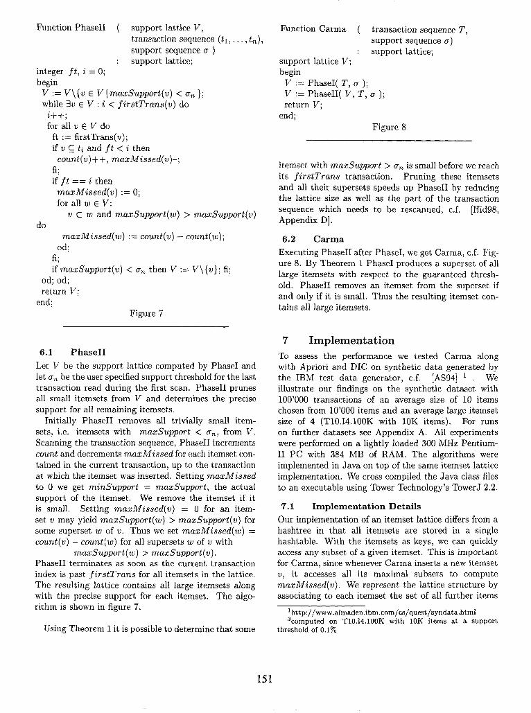
Function PhaseI( transaction sequence (ti, . . . , tn), support sequence c = (or,. . . , a,) ) : support lattice;

support lattice V; begin

v := (0); maxMissed := 0, firstTrans(w) := 0

count(w) := 0; for i from 1 to n do

// 1) Increment for all w E V with w c ti do count(v) + +;‘od; // 2) Insert for all w C ti with w $ V do

if VW c w : w E V and maxSupport > ui then v := vu {w}; firstTrans(w) := i; count(w) := 1; maxMissed :=

min{ [(i - l)avgi-i([ali-i)] + (~1 - 1, maxMissed + count(w) - 11 w C w };

if (w( == 1 then maxMissed := 0; fi; f-t

773) Prune if ( i % max{ [l/oil, 500) ) == 0 then

V := {w E V 1 maxSupport 2 (pi or lwl == 1); fi;

od; return V;

end; Figure 3

Then V is a support lattice relative to the support threshold

with c the maximal cardinality of a large itemset in T. For any itemset w

“I - l support,(v) > avgn(Taln)+- implies v E v. n

Proof: By double induction on c and n. For a de- tailed proof see [Hid98, Theorem 2, Appendix C].

We illustrate Theorem 1 and in particular the support threshold given by (3) in Subsection 5.4. We omitted any optimization in the definition of PhaseI. For exam- ple, the incrementation and insertion step can be ac- complished by traversing the support lattice once. We illustrate the algorithm itself on a simple example in the following Subsection 5.3.

5.3 Example

We illustrate in this subsection the Phase1 algorithm on a simple example, namely on the transaction sequence T = ({a, b}, {a, b, c}, {b, c}) and the support sequence o = (0.3, 0.9, 0.7), see Figure 4 below. As indicated we denote by the triple the three associated integers for each set in the support lattice V and by the interval the bounds on its support.

We initialize V to {0} and the associated integers of 0 to (O,O,O). Reading tl = {a, b} we first increment the count of 0, since 0 C tl. Because the empty set is the only strict subset of a singleton set and 1 = maxSupport(0) >_ 01, we add the singletons {a} and {b} to V. By maxMissed = 0 for all singleton sets, we set their associated integers to (O,l, 1). Since there is no set in V with maxSupport < 0.3, we can not prune an itemset from V and the first transaction is processed.

Reading t2 = {a, b, c} we first increment count for 0, {a} and {b}. As above we insert the singleton set {c}, setting maxMisssed to 0. Since {a, b} 2 t2 and {a}, {b} are elements of V with a maxSupport 2 02 = 0.9, we insert {a, b} in V. Since rcr] i = (0.3,0,0, . . .) we get awgi ([oli) = 0.3 and

[(Z - l)awg1( [glr)j + 2 - 1 = 1. Hence maxMissed({a,b}) = 1 by equality (2) of Subsection 5.2, since maxMissed(w)+count(w) = 2 for w = {a} and w = {b}. We set the associated integers of {a, b} to (1,2,1). W e note that maxSupport( {a, b}) = 1 is a sharp upper bound, since supportz({a, b}) = 1.

Reading t3 = {b, c} we increment the count of 8, {b} and {c}. We th en insert {b, c} since {b} and {c} are elements of V with maxSupport above the new user defined support threshold ~3 = 0.5. By [u)z = (0.9,0.9,0,0,.. .) we get awg2([o12) = 0.9 and hence [(3 - 1) . 0.91 + 2 - 1 = 2. Since maxMissed({c}) + count({c}) - 1 = 1 we get

maxMissed({b, c,}) = min(2, l} = 1. Because all itemsets have a maxsupport greater than 0.5 we can not remove any itemsets from the lattice. If ~3 was 0.7 instead of 0.5 we would not have inserted (6, c} while we could have removed {a, b}. However we could not have removed {c}, since our pruning strategy during PhaseI never removes singelton sets.

5.4 Changing Support Thresholds

We discuss in this subsection constant and changing support thresholds. Phase1 guarantees that all itemset with a support greater or equal to the support threshold given by Theorem 1 are included in the itemset lattice. We denote by the guaranteed support threshold this threshold, i.e.

149

0 v (O,O,O) v (O!o!l, NOI t,= 1 a, b I WI )

ot= 0.3

la) (b) (OJJ) WJ) 11911 IL11

( maxMissed, tkstlrans, count )

[ minSupport, maxSupport ]

constant support threshold

10000 20000 30000 40000 transaction

Figure 5

with D the support sequence, c the maximal cardinality of a large itemset and n the current transaction index.

First, suppose the user does not change the support threshold. Hence we have a constant support sequence 0 = (s, s, s, . . .) f or some s. By (4) and avg,( [aIn) = s Phase1 includes at tr.ansaction n all large itemsets with a support 2 s + ti Thus, the guaranteed threshold . s+ + converges to” t he user specified support threshold s as Phase1 scans the transaction sequence. To improve the speed of convergence, we run Phase1 with a lower threshold of s . 0.9 instead of s. As the guaranteed threshold reaches s, we increase the threshold again from s .0.9 to s, see Figure 5.

Next, consider changing support thresholds. Figure 6 depicts a scenario, where the user increases at transaction 5’000 the initial support threshold of 0.75% to 1.25% and then lowers it again to 1.0% at transaction 10’000. As above, we supply Phase1 with thresholds gi lower than the user specified threshold, whenever the guaranteed threshold does not equal the user specified threshold. We set cri, the support sequence supplied to Carma, to 0.9 ‘0.75% := 0.68% for i = 1, . ,4’999. The

Ia) (b) (O,W (0,1,21 ILlI WI

\/ f%bl WJ) KWll

Figure 4

(8) (b) (cl Kw) (OA3) WQ)

[0.66,0&i] [l,l] [O&6,0.66]

\/ \/ Ia,bJ tb,c) WJ) (L3J)

[0.33,0.661 [0.33,0.661

1.5

1.25

1

0.75

0.5

changing support threshold I I I , I

given by the user - supplied to Carma -----

,puaranteed by Carma .--.- . . . .

------I . . .-._ . . . . .._____

1 I I 1 I I

10000 20000 30000 40000 transaction

Figure 6

guaranteed threshold (4) drops quickly 3, reaching a value well below 1% at transaction 4’999. Since the new user specified threshold of 1.25% at transaction 5’000 is greater than l%, we have equality until transact:ion 9’999. Hence we set oi to 1.25% for i = 5’000,. . . ,9’9’99. As the user lowers the threshold to 1% we set ci to 0.9 . 1% = 0.9% from i = 10’000 until the guaranteed threshold reaches 1.0% at transaction 35’000. We reset (pi to 1% for all i > 35’000, since the user defined threshold remains at 1% from now on.

We note that the guaranteed threshold is an upper bound and thus a worst-case threshold. Typically, .a11 large itemsets are contained in the lattice well before the guaranteed threshold reaches the user specificed threshold.

6 Carma

In Subsection 6.1 we give a short description of PhaseHI, the algorithm for the second scan. We then combine in Subsection 6.2 Phase1 with Phase& yielding Carma.

3For this example we assumed that all large itemsets are of cardinality 10 or less, i.e. c = 10.

150

Function Phase11 ( support lattice V, transaction sequence (ti, . . . , tn), support sequence 0 )

: support lattice; integer ft, i = 0; begin

v := V\{w E v ( maxSupport < un }; while 3w E V : i < firstTrans(w) do

is+; for all w E V do

ft := firstTrans(v); if v G ti and ft < i then

count(w)++, maxMissed(w fi; if ft == i then

maxMissed := 0; for all w E V:

do v c w and maxSupport > maxSupport

maxMissed := count(w) - count(w); od;

fi; if maxSupport < gn then V := V\(w); fi;

od; od; return V;

end; Figure 7

6.1 Phase11

Let V be the support lattice computed by Phase1 and let (T, be the user specified support threshold for the last transaction read during the first scan. Phase11 prunes all small itemsets from V and determines the precise support for all remaining itemsets.

Initially Phase11 removes all trivially small item- sets, i.e. itemsets with maxsupport < un, from V. Scanning the transaction sequence, Phase11 increments count and decrements maxMissed for each itemset con- tained in the current transaction, up to the transaction at which the itemset was inserted. Setting maxMissed to 0 we get minsupport = maxsupport, the actual support of the itemset. We remove the itemset if it is small. Setting maxMissed = 0 for an item- set w may yield maxSupport > maxSupport for some superset w of v. Thus we set maxMissed = count(w) - count(w) for all supersets w of w with

maxSupport > maxSupport( Phase11 terminates as soon as the current transaction index is past firstTrans for all itemsets in the lattice. The resulting lattice contains all large itemsets along with the precise support for each itemset. The algo- rithm is shown in figure 7.

Using Theorem 1 it is possible to determine that some

Function Carma ( transaction sequence T, support sequence 0)

: support lattice; support lattice V; begin

V := PhaseI( T, cr ); V := PhaseII( V, T, cr ); return V;

end; Figure 8

itemset with maxsupport > un is small before we reach its firstTrans transaction. Pruning these itemsets and all their supersets speeds up Phase11 by reducing the lattice size as well as the part of the transaction sequence which needs to be rescanned, c.f. [Hid98, Appendix D].

6.2 Carma

Executing Phase11 after PhaseI, we get Carma, c.f. Fig- ure 8. By Theorem 1 Phase1 produces a superset of all large itemsets with respect to the guaranteed thresh- old. Phase11 removes an itemset from the superset if and only if it is small. Thus the resulting itemset con- tains all large itemsets.

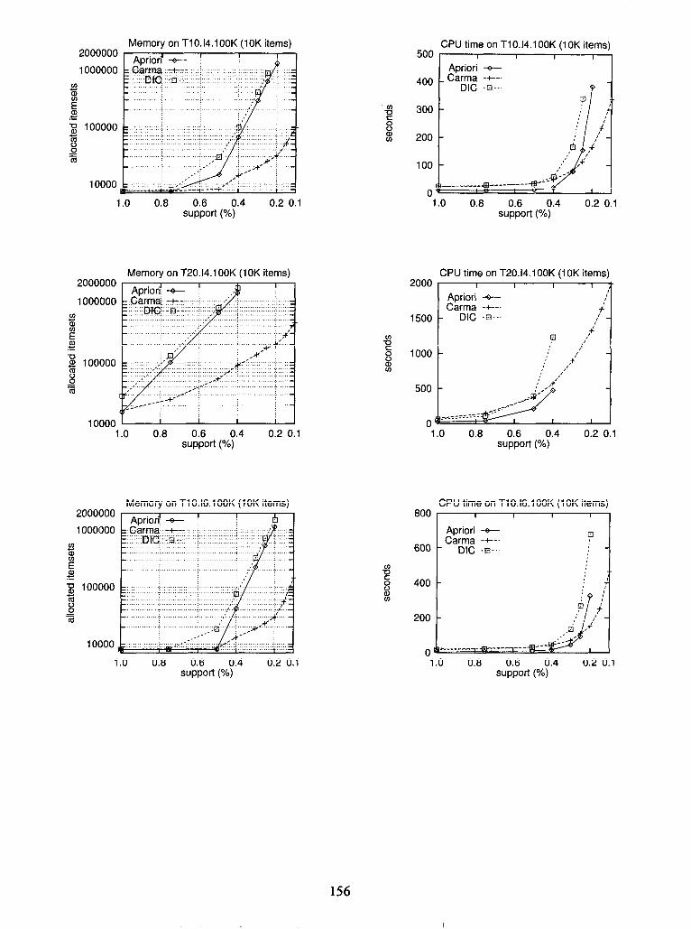
7 Implementation To assess the performance we tested Carma along with Apriori and DIC on synthetic data generated by the IBM test data generator, c.f. [AS941 1 We illustrate our findings on the synthetic dataset with 100’000 transactions of an average size of 10 items chosen from 10’000 items and an average large itemset size of 4 (T10.14.100K with 10K items). For runs on further datasets see Appendix A. All experiments were performed on a lightly loaded 300 MHz Pentium- II PC with 384 MB of RAM. The algorithms were implemented in Java on top of the same itemset lattice implementation. We cross compiled the Java class files to an executable using Tower Technology’s TowerJ 2.2.

7.1 Implementation Details

Our implementation of an itemset lattice differs from a hashtree in that all itemsets are stored in a single hashtable. With the itemsets as keys, we can quickly access any subset of a given itemset. This is important for Carma, since whenever Carma inserts a new itemset w, it accesses all its maximal subsets to compute maxMissed( We represent the lattice structure by associating to each itemset the set of all further items

‘http://www.almaden,ibm.com/cs/quest/syndata.html 3computed on T10.14.100K with 10K items at a support

threshold of 0.1%

151

Memory on Ti 0.14.1 OOK (10K items) 2000000

1000000

s % E 22 2 100000

: 74

10000 B

500 , CPU time on Tl 0.14.1 OOK (1 OK items)

, I I I ,

1 .o 0.8 0.6 0.4 0.2 0.1 -1.0 0.8 0.6 0.4 0.2 0.1 support (%) Figure 9

support (%) Figure 10

large itemsets in lattice

In ‘iii 90 unfiltered lattice +-

E filtered lattice --+

c 80 i% 3 = 70 RI 5 9 0 60

20000 40000 60000 80000 transaction Figure 113

appearing in any of its supersets, c.f. [Bay98]. As in the case of a hashtree, we need only one hashtable access to pass from an itemset to one of its minimal supersets. Thus we can enumerate all subsets of a scanned transaction, which are contained in the lattice, as quickly as in a hashtree.

Our implementation of Carma diverges from the pseudo-code given in Subsection 5.2 only in that we perform the Phase1 incrementation and insertion step simultaneously, enum.erating the subsets of a scanned transaction once.

Apriori and DIC were implemented as described in [AS941 and [BMUTSi) respectively. For DIC we chose a blocksize of 15000, which we found to be fastest.

7.2 Relative Performance

To compare Carma with Apriori and DIC we ran all three algorithms on a range of datasets and (constant) support thresholds. In this subsection we illustrate our results on the ‘TlO.14.100K dataset with 10K items. For support thresholds of 0.5% and above Apriori outperformed Carma and DIC. We attribute the superior speed of Apriori for these thresholds to the observation that, for example, at 0.75% only 171 large itemsets existed and all large itemsets were I-itemsets. Thus Apriori completes in 2 scans allocating only 300

size of support intervals

average in unfiltered lattice -+- median in unfiltered lattice -t--

median in filtered lattice ++--

0.075

0.050

0.025

0.000 20000 40000 60000 80000

transaction Figure 123

P-itemsets. As the support threshold was lowered to 0.25% (0.1%) the number of large l-itemsets increased to 1131 (3509) and the maximal cardinality to 4 (9). We were not able to run Apriori (DIC) with thresholds below 0.2% (0.25%), since the allocated itemsets did not fit into main memory anymore. At 0.15% (0.1%) Apriori would have allocated 2.8 million (6.2 million) 2-itemsets2, while Carma required only 51001 (97872) itemsets. We note that DIC always allocates at least as many itemsets as Apriori. At 0.25% and below Carma outperformed Apriori and DIC.

We attribute the better performance of Carma over Apriori to the 4 scans needed by Apriori while Carma completed in 1.1 scans. We attribute the bet& performance of Carma over DIC to the 2 scans needed by DIC as well as to the 35 times smaller lattice maintained by Carma, since both algorithms traverse their lattices in regular intervals.

7.3 Support Intervals

Phase1 maintains a superset of the large itemsets in the scanned part of the transaction sequence, bu.t not necessarily a superset for the full transaction sequence. First, we wanted to determine the percentage

2The number of candidate P-itemsets which Apriori allocates is given by the number of large l-itemsets over 2.

152

of all large itemsets, i.e. with respect to the full transaction sequence, contained in the lattice as Phase1 proceeds. After scanning 20000 (40000) transactions at a threshold of 0.1% Carma included 99.3% (99.8%) of all large itemsets in its lattice, see figure 11.

Between two pruning steps Phase1 replaced up to 50% of all itemsets. The vast majority (typically > 95%) of itemsets in the lattice eventually turned out to be small. As we scan the transaction sequence we would present a large number of association rules to the user based on itemsets which are likely to be small. To exclude those itemsets from the rule generation, which are likely to be small, we filtered out all itemsets which were inserted during the last 15% of the transaction sequence, e.g. at transaction 20000 we filter out all itemsets which were inserted at transaction 17000 or later. The filtered lattice still contained 93.9% (97.8%) of all large itemsets, after scanning 20000 (40000) transactions respectively, c.f. figure 9. At the same time the size of the filtered lattice was reduced to 32.6% (16.0%) of its original size.

Recall that the support interval of an itemset in the lattice is given by its minSupport and maxSupport. Next, we wanted to determine how the size of the support intervals, i.e. maxSupport - minSupport, in the filtered lattice evolve as Phase1 proceeds. After scanning 20000 (40000) transactions at a threshold of 0.1% the average interval size in the filtered lattice was 0.042% (0.032%), while 50% of all itemsets in the lattice had an interval size below 0.004% (0.002%), c.f. figure 12.

8 Conclusion

We presented Carma, a novel algorithm to compute large itemsets online. It continuously produces large itemsets along with a shrinking support interval for each itemset. It allows the user to change the support threshold anytime during the first scan and always completes in at most 2 scans.

We implemented Carma and compared it to Apriori and DIC. While not being faster in general, Carma out- performs Apriori and DIC on low support thresholds. We attributed this to the observation that Carma is typically an order of magnitude more memory efficient. We showed that Carma’s itemset lattice quickly approx- imates a superset of all large itemsets while the sizes of the corresponding support intervals shrink rapidly. We also showed that Carma readily computes large itemsets in cases which are intractable for Apriori or DIC.

An interesting feature of the algorithm is that the second scan ist not needed, whenever the shrinking sup- port intervals suffice. Thus Phase1 can be used to con- tinuously compute large itemsets from a transaction se- quence read from a network, generalizing incremental updates and not requiring local storage.

Acknowledgement: I would like to thank Joseph M. Hellerstein, UC Berkeley, for his inspiration, guid- ance and support. I am thankful to Ron Avnur for the many discussions and to Retus Sgier, for his help and suggestions. I would like to thank Rajeev Motwani, Stanford University, for pointing out the applicability of Carma to transaction sequences read from a network. Also, I would like to thank Ramakrishnan Srikant, IBM Almaden Research Center, for his remarks on speeding up the convergence of the support thresholds.

References

[AIS93]

[AS941

[AY97]

[AY98]

Pay981

[BMUT97]

[CHNW96]

R. Agrawal, T. Imielinski, and A. Swami. Mining association rules between sets of items in large databases. In Proc. of the ACM SIGMOD Conference on Manage- ment of Data, pages 207-216, Washington, D.C., May 1993.

R. Agrawal and R. Srikant. Fast algorithms for mining association rules. In Proc. of the 20th Int’l Conf. on Very Large Databases, Santiago, Chile, Sept. 1994.

Charu C. Aggarwal and Philip S. Yu. On- line generation of association rules. Tech- nical Report RC 20899 (92609), IBM Re- search Division, T.J. Watson Research Center, Yorktown Heights, NY, June 1997.

Charu C. Aggarwal and Philip S. Yu. Mining large itemsets for association rules. Bulletin of the IEEE Computer Society Technical Comittee on Data Engineering, pages 23-31, March 1998.

R. J. Bayardo Jr. Efficiently mining long patterns from databases. In Proc. of the 1998 ACM-SIGMOD International Conference on Management of Data, pages 85-93, Seattle, June 1998.

Sergey Brin, Rajeev Motwani, Jeffrey D. Ullman, and Shalom Tsur. Dynamic itemset counting and implication rules for market basket data. In Proceedings of the ACM SIGMOD International Confer- ence on Management of Data, volume 26,2 of SIGMOD Record, pages 255-264, New York, May 13th-15th 1997. ACM Press.

D. Cheung, J. Han, V. Ng, and C.Y. Wong. Maintenance of discovered association rules in large databases: An incremental updat- ing technique. In Proc. of 1996 Int’l Conf. on Data Engineering (ICDE’96), New Or- leans, Louisiana, USA, Feb. 1996.

153

[CLK97]

[He1961

[HHW97]

[Hid981

[SON951

[TBAR97]

[Toi96]

[ZPLO96]

David W. L. Cheung, S.D. Lee, and Ben- jamin Kao. A general incremental tech- nique for maintaining discovered associa- tion rules. In Proceedings of the Fifth Inter- national Conference On Database Systems For Advanced Applications, pages 185-194, Melbourne, Australia, March 1997.

Joseph M. Hellerstein. The case for online aggregation. Technical Report UCB//CSD-96-908, EECS Computer Sci- ence Divison, University of California at Berkeley, 1996.

Josepih M. Hellerstein, Peter J. Haas, and Helen J. Wang. Online aggregation. SIG- MOD ‘97, 1997.

C. Hidber. Online Association Rule Min- ing. Technical Report TR-98-033, Interna- tional Computer Science Institute, Berke- ley, CA, September 1998. an earlier version appeared as technical report UCB//CSD- 98-1004 of the Department of Electrical En- gineering and Computer Science, Univer- sity of California at Berkeley.

A. Savasere, E. Omiecinski, and S. Na- vathe. An efficient algorithm for mining association rules in large databases. In Pro- ceedings of the Very Large Data Base Con- ference, September 1995.

Shiby Thomas, Sreenath Bodagala, Khaled Alsabt:i, and Sanjay Ranka. An efficient algorithm for the incremental updation of association rules in large databases. In Proceedings of the 3rd International conference on Knowledge Discovery and Data lllining (KDD 97), New Port Beach, California, August 1997.

Hannu Toivonen. Sampling large databases for association rules. In T. M. Vijayara- man, A.lejandro P. Buchmann, C. Mohan, and Nandlal L. Sarda, editors, VLDB’96, Proceedings of 22th International Confer- ence on Very Large Data Bases, Mumbai (Bombay), India, September 1996. Morgan Kaufmann.

Mohammed Javeed Zaki, Srinivasan Parthasarathy, Wei Li, and Mitsunori Ogihara.. Evaluation of sampling for data mining of association rules. Technical Report 617, Computer Science Dept., U. Rochester, May 1996.

154

A Performance Figures

1000000

g 100000

8 = m

Memory on T10.14.1 OOK (I K items)

Aprior; + ! \ I

=.c;a~m;l:::~~:::::i::::.:::.::::::::i: :::::.:::::.:.:/::.:::= =ii:ji:jR~:-~--:::.::‘:::::::::.::::::.~::::.::::::.:::::~:::::= . . . . . . .,.. .: ,... .,

2000000

1000000

22 I E a .e

p 100000

8 = m

Memory on Ti 0.14.1 OOK (2K items)

1.0 0.8 0.2 0.1

Memory on TlO.14.1 OOK (5K items)

1.0 0.8 0.4 s”;;ort (%)

0.2 0.1

1000 , CPU time on Tl0.14.lOOK (1K items)

I , I I I

600

0.8 0.6 0.4 0.2 0.1 support (%)

1000 , CPU time on TlO.14.1 OOK (2K items)

I 1 I 1 1

R zl 600 s

Q 400

200

0 -1.0 0.8 0.4

su;;ort (“x2) 0.2 0.1

CPU time on TlO.14.1 OOK (5K items)

;;i mj

400

300

200

100

n I I

-1 .o 0.8 0.6 0.4 0.2 0.1 support (%)

155

2000000

1000000

z?

i?i E a

‘g 100000

8 0 = co

10000

2000000

1000000 In 5 if d -0 2 100000

2 = m

Memory on Tl 0.14.1 OOK (1 OK items)

,, ,:. . ..-..:-...-,I; 1,. : ::: : .:.:

i~~~:i

j ;. ..;;.a .;... ;;i;vy..

,;;..llz+l:.: : : ::.: .,::,,::,... :. :.:.

1.0 0.8 0.6 0.4 0.2 0.1 support (%)

Memorv on T20.14.1 OOK (1 OK items)

10000-i i i i 1 1.0 0.8 suodport 0.4 0.2 0.1

(%)

2000000

1000000

22 s E a

‘g 100000

2 = ([I

10000

Memory on Tl 0.16.1 OOK (1 OK items)

~I

.carmgy* .::::; :..::::::: :::::: i :::.::::::::.: i:< :.::: :::.:.: lFj*.r:- n, . ..e.~-i::.,::~iiiiiiiiiiiiiiiii ::~._:::::~, .:; ..:::.

1.0 0.8 0.6 0.4 0.2 0.1 support (%)

500 CPU time on T10.14.1 OOK (1 OK items)

I I I I Aoriori *

-1.0 0.8 0.4 su;;ort (%)

0.2 0.1

CPU time on T20.14.lOOK (10K items)

y;;: piigg-7’

I’

2 0 /+

8 1000 - f

% i

: ,’

500 -

I -1.0 0.8 0.4

su”pb”ort pa) 0.2 0.1

CPU time on T10.16.lOOK (10K items)

1;; pg--q

n “1 .o 0.8 0.4

suopbort (%) 0.2 0.1

156