149
Online Kernel Learning Jose C. Principe Jose C. Principe Computational NeuroEngineering Laboratory (CNEL) Ui it f Fl id University of Florida [email protected], [email protected]

Online Kernel Learningg
Jose C. PrincipeJose C. Principe
Computational NeuroEngineering Laboratory (CNEL)U i it f Fl idUniversity of Florida

AcknowledgmentsAcknowledgments
Dr. Weifeng Liu, Amazon
D B d ChDr. Badong Chen Tsinghua University and Post Doc CNEL
NSF ECS – 0300340 and 0601271 (N i i )(Neuroengineering program)

O tliOutline
1 Optimal adaptive signal processing fundamentals1. Optimal adaptive signal processing fundamentalsLearning strategyLinear adaptive filtersLinear adaptive filters
2. Least-mean-square in kernel spaceWell-posedness analysis of KLMS
3. Affine projection algorithms in kernel space4. Extended recursive least squares in kernel space5. Active learning in kernel adaptive filtering

Wiley Book (2010)Wiley Book (2010)
Papers are available atPapers are available atwww.cnel.ufl.edu
Part 1: Optimal adaptive signal p p gprocessing fundamentals

Machine LearningProblem Definition for Optimal System DesignProblem Definition for Optimal System Design
Assumption: Examples are drawn independently from an unknown probability distribution P(u y) that represents theunknown probability distribution P(u, y) that represents the rules of Nature.Expected Risk:Find f∗ that minimizes R(f) among all functions
= ),()),(()( yudPyufLfR
Find f∗ that minimizes R(f) among all functions.But we use a mapper class F and in general The best we can have is that minimizes R(f).
Ff ∉*
FfF ∈*
P(u, y) is also unknown by definition.Empirical Risk: Instead we compute that minimizes Rn(f).
=i
iiN yufLNfR )),((/1)(ˆ
FfN ∈p n( )Vapnik-Chervonenkis theory tells us when this will work, but the optimization is computationally costly.Exact estimation of fN is done thru optimization
fN
Exact estimation of fN is done thru optimization.

Machine Learning Strategy
The optimality conditions in learning and optimization th i th ti ll d itheories are mathematically driven:
Learning theory favors cost functions that ensure a fast estimation rate when the number of examples increases (small estimation error bound)bound).Optimization theory favors super-linear algorithms (small approximation error bound)
What about the computational cost of these optimal solutions inWhat about the computational cost of these optimal solutions, in particular when the data sets are huge?Estimation error will be small, but can not afford super linear solutions:solutions: Algorithmic complexity should be as close as possible to O(N).

Statistic Signal Processing Adaptive Filtering PerspectiveAdaptive Filtering Perspective
Adaptive filtering also seeks optimal models for time series. The linear model is well understood and so widely appliedThe linear model is well understood and so widely applied. Optimal linear filtering is regression in functional spaces, where the user controls the size of the space by choosing the model orderorder. Problems are fourfold:
Application conditions may be non stationary, i.e. the model must be continuously adapting to track changesbe continuously adapting to track changes. In many important applications data arrives in real time, one sample at a time, so on-line learning methods are necessary. Optimal algorithms must obey physical constrains, FLOPS, memory,Optimal algorithms must obey physical constrains, FLOPS, memory, response time, battery power. Unclear how to go beyond the linear model.
Although the optimalilty problem is the same as in machine g p y plearning, constraints make the computational problem different.

Machine Learning+Statistical SP
Since achievable solutions are never optimal (non-reachable set of functions, empirical risk), goal should be to get quickly to the
Change the Design Strategy
of functions, empirical risk), goal should be to get quickly to the neighborhood of the optimal solution to save computation.The two types of errors are
Approximation error*** Approximation errorEstimation error
)()(
)()()()(*
***
FN
FN
fRfR
fRfRfRfR
−+
+−=−
But fN is difficult to obtain, so why not create a third error (Optimization Error) to approximate the optimal solution
ρ=− )~()( NN fRfRprovided it is computationally simpler to obtain.
So the problem is to find F, N and ρ for each application.
Leon Bottou: The Tradeoffs of Large Scale Learning, NIPS 2007 tutorial

Learning Strategy in Biologyg gy gy
In Biology optimality is stated in relative terms: the best possible response within a fixed time and with the available (finite)response within a fixed time and with the available (finite) resources. Biological learning shares both constraints of small and large learning theory problems because it is limited by the number oflearning theory problems, because it is limited by the number of samples and also by the computation time.Design strategies for optimal signal processing are similar to the biological framework than to the machine learning frameworkbiological framework than to the machine learning framework.What matters is “how much the error decreases per sample for a fixed memory/ flop cost”It is therefore no surprise that the most successful algorithm inIt is therefore no surprise that the most successful algorithm in adaptive signal processing is the least mean square algorithm (LMS) which never reaches the optimal solution, but is O(L) and tracks continuously the optimal solution!tracks continuously the optimal solution!

Extensions to Nonlinear Systemsy
Many algorithms exist to solve the on-line linear regressionproblem:p ob e
LMS stochastic gradient descentLMS-Newton handles eigenvalue spread, but is expensiveRecursive Least Squares (RLS) tracks the optimal solution with the available data.
Nonlinear solutions either append nonlinearities to linear filters (not optimal) or require the availability of all data (Volterra, neural networks) and are not practicalnetworks) and are not practical. Kernel based methods offers a very interesting alternative to neural networks.
Provided that the adaptation algorithm is written as an inner product,Provided that the adaptation algorithm is written as an inner product, one can take advantage of the “kernel trick”. Nonlinear filters in the input space are obtained. The primary advantage of doing gradient descent learning in RKHS i th t th f f i till d ti this that the performance surface is still quadratic, so there are no local minima, while the filter now is nonlinear in the input space.
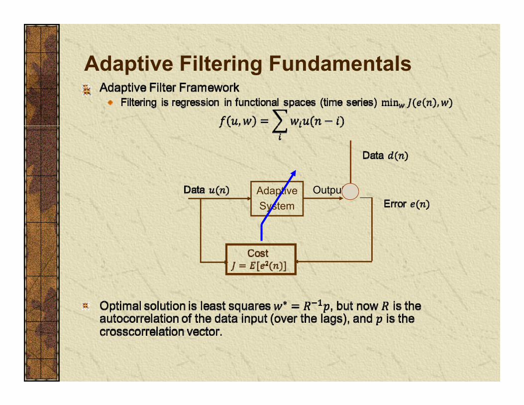
Adaptive Filtering Fundamentalsp g
AdaptiveSystem
Output

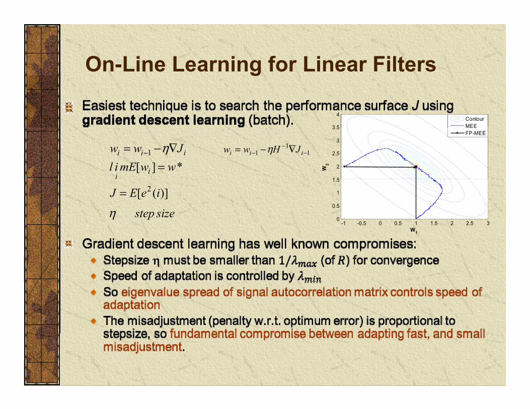
On-Line Learning for Linear Filtersg
Notation:
iwiu ( )y i wi weight estimate at time i (vector) (dim = l)
ui input at time i (vector)
Σ( )e i
e(i) estimation error at time i (scalar)
d(i) desired response at time i ( l )
Th t ti t i t d i
Σ
( )d i
(scalar)
ei estimation error at iteration i (vector)
d d i d t it tiThe current estimate is computed in terms of the previous estimate, , as:
iw
1i i i iw w G e−= +1iw −
di desired response at iteration i (vector)
Gi capital letter matrix
ei is the model prediction error arising from the use of wi-1 and Gi is a Gain term
On-Line Learning for Linear Filtersg
3 5
4ContourMEE
wwmEilJww
ii
iii η*][
1
=∇−= −
W2
1 5
2
2.5
3
3.5 MEEFP-MEE
11
1 −−
− ∇−= iii JHww η
sizestep
ieEJi
η)]([ 2=
W-1 -0.5 0 0.5 1 1.5 2 2.5 3
0
0.5
1
1.5
W1
On-Line Learning for Linear Filtersg
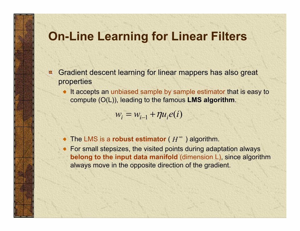
Gradient descent learning for linear mappers has also greatGradient descent learning for linear mappers has also great properties
It accepts an unbiased sample by sample estimator that is easy to compute (O(L)) leading to the famous LMS algorithmcompute (O(L)), leading to the famous LMS algorithm.
)(1 ieuww iii η+= −
The LMS is a robust estimator ( ) algorithm. For small stepsizes, the visited points during adaptation always belong to the input data manifold (dimension L), since algorithm
∞H
be o g to t e put data a o d (d e s o ), s ce a go talways move in the opposite direction of the gradient.

On-Line Learning for Non-Linear Filters?g
Can we generalize to nonlinear models?1i i i iw w G e−= +g
and create incrementally the nonlinear mapping?
Ty w u= ( )y f u=y pp g
( )y i
iiii eGff += −1
ifiu ( )y i
Σ( )e i
Σ
( )d i

Part 2: Least-mean-squares in kernel qspace
Non-Linear Methods - TraditionalNon Linear Methods Traditional(Fixed topologies)
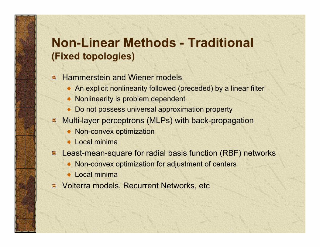
Hammerstein and Wiener modelsHammerstein and Wiener modelsAn explicit nonlinearity followed (preceded) by a linear filterNonlinearity is problem dependentDo not possess universal approximation propertyDo not possess universal approximation property
Multi-layer perceptrons (MLPs) with back-propagationNon-convex optimizationL l i iLocal minima
Least-mean-square for radial basis function (RBF) networks Non-convex optimization for adjustment of centersLocal minima
Volterra models, Recurrent Networks, etc

Non-linear Methods with kernels
Universal approximation property (kernel dependent)Convex optimization (no local minima)Convex optimization (no local minima)Still easy to compute (kernel trick)But require regularizationSequential (On-line) Learning with KernelsSequential (On line) Learning with Kernels
(Platt 1991) Resource-allocating networksHeuristicNo convergence and well-posedness analysis
(Frieb 1999) Kernel adalineFormulated in a batch modewell-posedness not guaranteedg
(Kivinen 2004) Regularized kernel LMSwith explicit regularizationSolution is usually biased
(Engel 2004) Kernel Recursive Least Squares(Engel 2004) Kernel Recursive Least-Squares (Vaerenbergh 2006) Sliding-window kernel recursive least-squares

Neural Networks versus Kernel Filters
ANNs Kernel filters
Universal Approximators YES YESC O ti i ti NO YESConvex Optimization NO YESModel Topology grows with data NO YES
Require Explicit Regularization NO YES/NO (KLMS)Require Explicit Regularization NO YES/NO (KLMS)
Online Learning YES YES
Computational Complexity LOW MEDIUM
ANNs are semi-parametric, nonlinear approximatorsKernel filters are non-parametric, nonlinear approximatorsp , pp
Kernel Methods
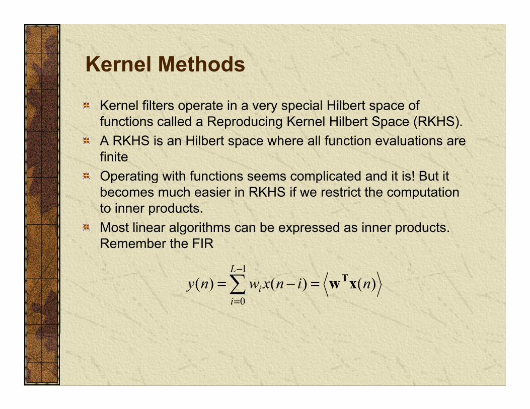
Kernel filters operate in a very special Hilbert space of functions called a Reproducing Kernel Hilbert Space (RKHS).p g p ( )A RKHS is an Hilbert space where all function evaluations are finiteOperating with functions seems complicated and it is! But itOperating with functions seems complicated and it is! But it becomes much easier in RKHS if we restrict the computation to inner products. Most linear algorithms can be expressed as inner products
)()()(1
ninxwnyL
xwT−
Most linear algorithms can be expressed as inner products. Remember the FIR
)()()(0
ninxwnyi
i xw=−==

Kernel MethodsMoore-Aronszajn theorem
Every symmetric positive definite function of two real variables in E κ(x,y) defines a unique Reproducing Kernel Hilbert Space (RKHS).
κκ
HxfxfHfExIIHxExI
>=<∈∀∈∀∈∈∀
)(.,,)(,)()(.,)(
Mercer’s theoremLet κ(x,y) be symmetric positive definite. The kernel can be
)exp(),( 2yxhyx −−=κκHfff )( ,,)(,)(
expanded in the series
Construct the transform as 1
( , ) ( ) ( )m
i i ii
x y x yκ λϕ ϕ=
=
Inner product
( ) ( ) ( )x y x yϕ ϕ κ, = ,
1 1 2 2( ) [ ( ), ( ),..., ( )]Tm mx x x xϕ λ ϕ λ ϕ λ ϕ=
( ) ( ) ( )y yϕ ϕ, ,

Kernel methods
Mate L., Hilbert Space Methods in Science and Engineering, A. Hildger, 1989Berlinet A., and Thomas-Agnan C., “Reproducing kernel Hilbert Spaces in probability and Statistics, Kluwer 2004

Basic idea of on-line kernel filteringg
Transform data into a high dimensional feature space Construct a linear model in the feature space F
: ( )i iuϕ ϕ=Construct a linear model in the feature space F
, ( ) Fy uϕ= Ω
Adapt iteratively parameters with gradient information
Compute the outputiii J∇+Ω=Ω − η1
p p
Universal approximation theorem 1( ) , ( ) ( , )
im
i i F j jj
f u u a u cϕ κ=
= Ω =Universal approximation theorem
For the Gaussian kernel and a sufficient large mi, fi(u) can approximate any continuous input-output mapping arbitrarily close in the Lp norm.
j
the Lp norm.

Growing network structure
1 ( ) ( )i i ie i uη ϕ−Ω = Ω +
1
1 ( ) ( , )i i if f e i uη κ−= + ⋅ mi

Kernel Least-Mean-Square (KLMS)q ( )
Least-mean-square
Transform data into a high dimensional feature space F
011 )()()( wuwidieieuww iTiiii −− −=+= η
: ( )i iuϕ ϕ=
0
1
0( ) ( ) , ( )i i Fe i d i uϕ−
Ω == − Ω 0 0
(1) (1) ( ) (1)e d u dϕΩ =
= Ω =
1 ( ) ( )i i iu e iηϕ−Ω = Ω +
( ) ( )i
jΩ
0 1
1 0 1 1 1
1 2
(1) (1) , ( ) (1)( ) (1) ( )
(2) (2) , ( )
F
F
e d u du e a u
e d u
ϕηϕ ϕ
ϕ
= − Ω =Ω = Ω + =
= − Ω
1( ) ( )i j
j
e j uη ϕ=
Ω =( ) , ( ) ( ) ( , )
i
i i F jf u u e j u uϕ η κ= Ω =
1 1 2
1 1 2
2 1 2
(2) ( ), ( )(2) ( , )
( ) (2)
Fd a u ud a u u
u e
ϕ ϕκ
ηϕ
= − = −
Ω = Ω +
RBF Centers are the samples, and Weights are the errors!1
( ) , ( ) ( ) ( , )i i F jj
f jϕ η=
1 1 2 2( ) ( )
...a u a uϕ ϕ= +

Kernel Least-Mean-Square (KLMS)( )
) )(()(1
jjfi−
),.)(()(
1
11 jjef
i
ji uκη=
−
=−
))(()()(
))(),(()())((1
1
fd
ijjeifj
i uuu κη==
− ))(()()( 1 ifidie i u−= −
),.)(()(1 iieff ii uκη+= −
Free Parameters in KLMS
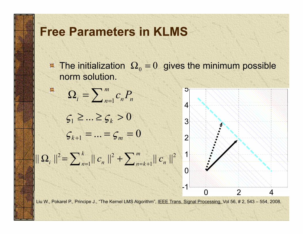
The initialization gives the minimum possible 00 =Ωnorm solution.
1
mi n nn
c P=
Ω =4
51n
3
4
1 ... 00
kς ςς ς≥ ≥ >
2 2 2|| || || || || ||k mi c cΩ = + 1
21 ... 0k mς ς+ = = =
1 1|| || || || || ||i n nn n k
c c= = +
Ω +
0 2 4-1
0
0 2 4Liu W., Pokarel P., Principe J., “The Kernel LMS Algorithm”, IEEE Trans. Signal Processing, Vol 56, # 2, 543 – 554, 2008.

Free Parameters in KLMS Step size
T diti l i d i LMS till li hTraditional wisdom in LMS still applies here.
NN
=
=< N
jjj
Ntr
N
1))(),((][ uuG κ
ηϕ
where is the Gram matrix, and N its dimensionality.For translation invariant kernels, κ(u(j),u(j))=g0, is a
ϕG
constant independent of the data. The Misadjustment is therefore ][
2 ϕη GtrN
M =

Free Parameters in KLMS Rule of Thumb for h
Although KLMS is not kernel density estimation, these rules of thumb still provide a starting point. Silverman’s rule can be applied
where σ is the input data s d R is the interquartile N{ } )5/(134.1/,min06.1 LNRh −= σ
where σ is the input data s.d., R is the interquartile, N is the number of samples and L is the dimension.Alternatively: take a look at the dynamic range of the y y gdata, assume it uniformly distributed and select h to put 10 samples in 3 σ.

Free Parameters in KLMSKernel DesignThe Kernel defines the inner product in RKHSThe Kernel defines the inner product in RKHS
Any positive definite function (Gaussian, polynomial, Laplacian, etc.), but we should choose a kernel that yields a class of functions that allows universal approximation. A strictly positive definite function is preferredA strictly positive definite function is preferred because it will yield universal mappers (Gaussian, Laplacian).
See Sriperumbudur et al, On the Relation Between Universality, Characteristic Kernels and RKHS Embedding ofMeasures, AISTATS 2010

Free Parameters in KLMS Kernel Design
Estimate and minimize the generalization error e gEstimate and minimize the generalization error, e.g. cross validation
Establish and minimize a generalization error upper bound, e.g. VC dimension
Estimate and maximize the posterior probability of the model given the data using Bayesian inferencethe model given the data using Bayesian inference
Free Parameters in KLMS Bayesian model selection
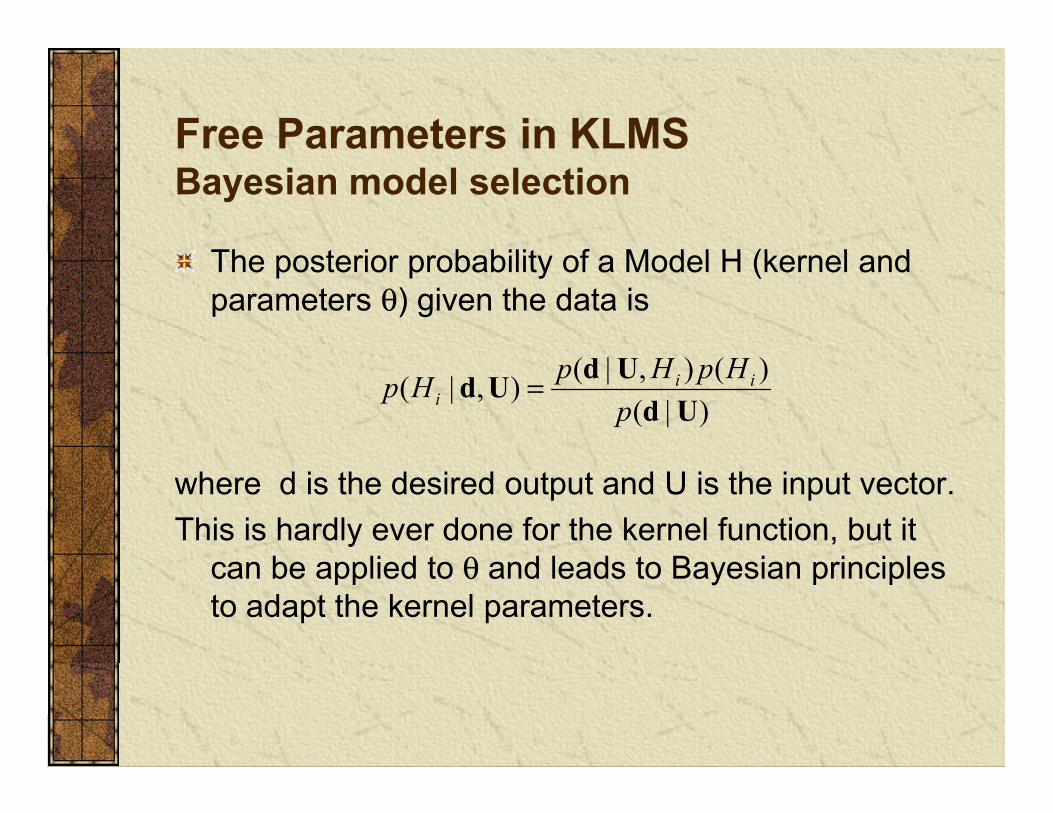
Th t i b bilit f M d l H (k l dThe posterior probability of a Model H (kernel and parameters θ) given the data is
)|()(),|(),|(
UdUdUdp
HpHpHp iii =
where d is the desired output and U is the input vector.This is hardly ever done for the kernel function, but it
b li d t θ d l d t B i i i lcan be applied to θ and leads to Bayesian principles to adapt the kernel parameters.

Free Parameters in KLMS Maximal marginal likelihood
)]2log(2log21)(21[)( 212 πσσθ
NxamHJ nnT
i −+−+−= − IGdIGd

SparsificationSparsification
Filter size increases linearly with samples!Filter size increases linearly with samples! If RKHS is compact and the environment stationary, we see that there is no need to keep increasing the p gfilter size.Issue is that we would like to implement it on-line! Two ways to cope with growth:
Novelty CriterionApproximate Linear DependencyApproximate Linear Dependency
First is very simple and intuitive to implement.
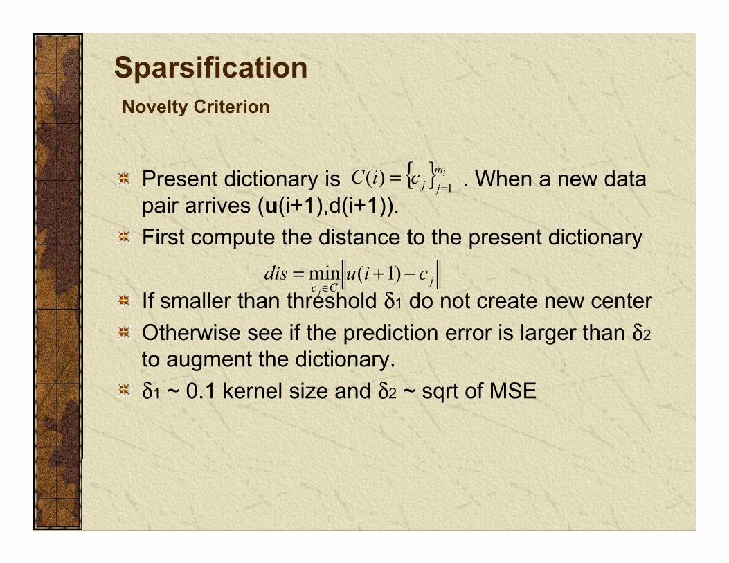
SparsificationNovelty CriterionNovelty Criterion
Present dictionary is When a new data{ } imciC )(Present dictionary is . When a new data pair arrives (u(i+1),d(i+1)).First compute the distance to the present dictionary
{ } i
jjciC1
)(=
=
p p y
If smaller than threshold δ1 do not create new centerjCc
ciudisj
−+=∈
)1(min
Otherwise see if the prediction error is larger than δ2
to augment the dictionary. δ1 0 1 kernel size and δ2 sqrt of MSEδ1 ~ 0.1 kernel size and δ2 ~ sqrt of MSE

SparsificationApproximate Linear DependencyApproximate Linear Dependency
Engel proposed to estimate the distance to the linearEngel proposed to estimate the distance to the linear span of the centers, i.e. compute
)())1((min jC j cbiudis −+= ϕϕWhich can be estimated by
)())(( jCc jb j ∈∨
ϕϕ
)1()()1())1(),1(( 12 ++−++= − iiiiidis T hGhuuκ
Only increase dictionary if dis larger than thresholdComplexity is O(m2)E t ti t i KRLS (di (i 1))Easy to estimate in KRLS (dis~r(i+1))Can simplify the sum to the nearest center, and it defaults to NCdefaults to NC
)())1((min, jCcb
ciudisj
ϕϕ −+=∈∨

KLMS- Mackey-Glass Predictiony30
)(1)(2.0)(1.0)( 10 =
−+−+−= τττ
txtxtxtx
LMSη=0.2KLMSa=1, η=0.2

Regularization worsens performanceg p

Performance Growth tradeoff
δ1=0.1, δ2=0.05η=0.1, a=1η
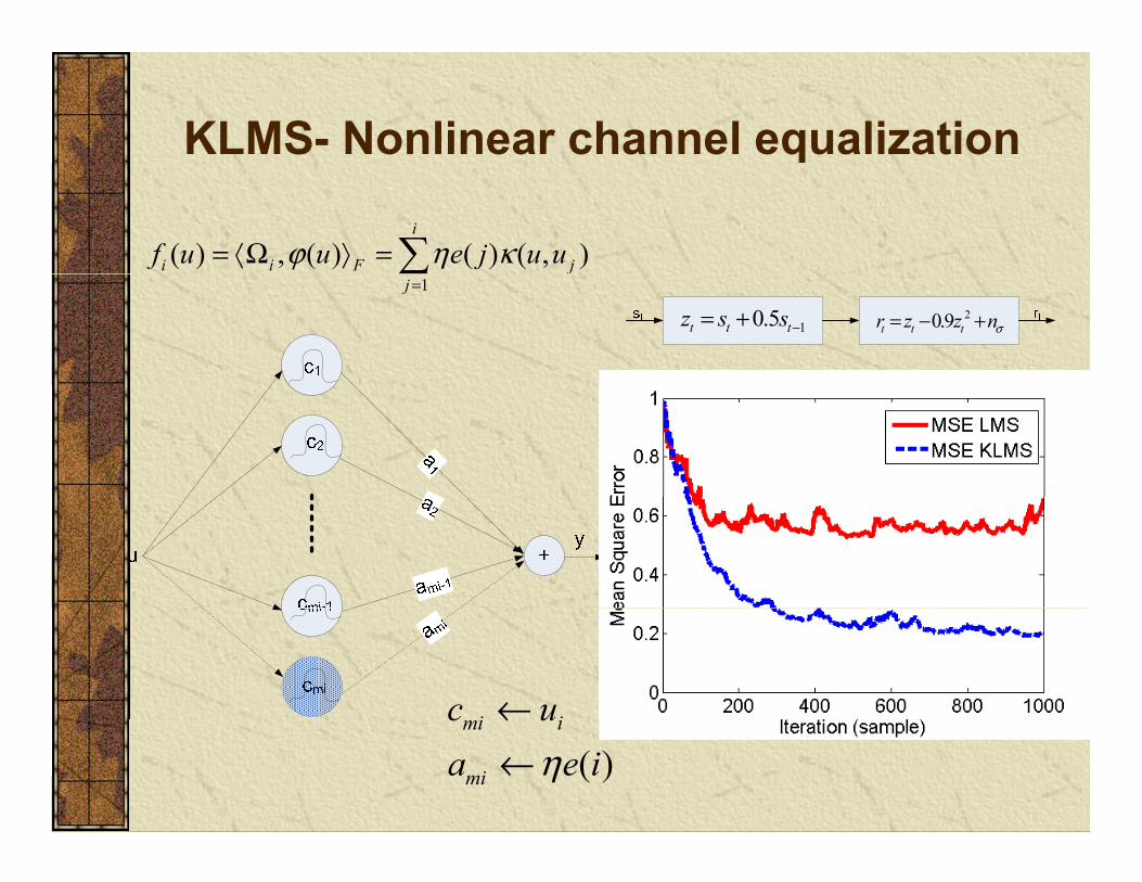
KLMS- Nonlinear channel equalization
( ) , ( ) ( ) ( , )i
i i F jf u u e j u uϕ η κ= Ω =1j=
10.5t t tz s s −= + 20.9t t tr z z nσ= − +
i ic u←( )
mi i
mi
c ua e iη←←
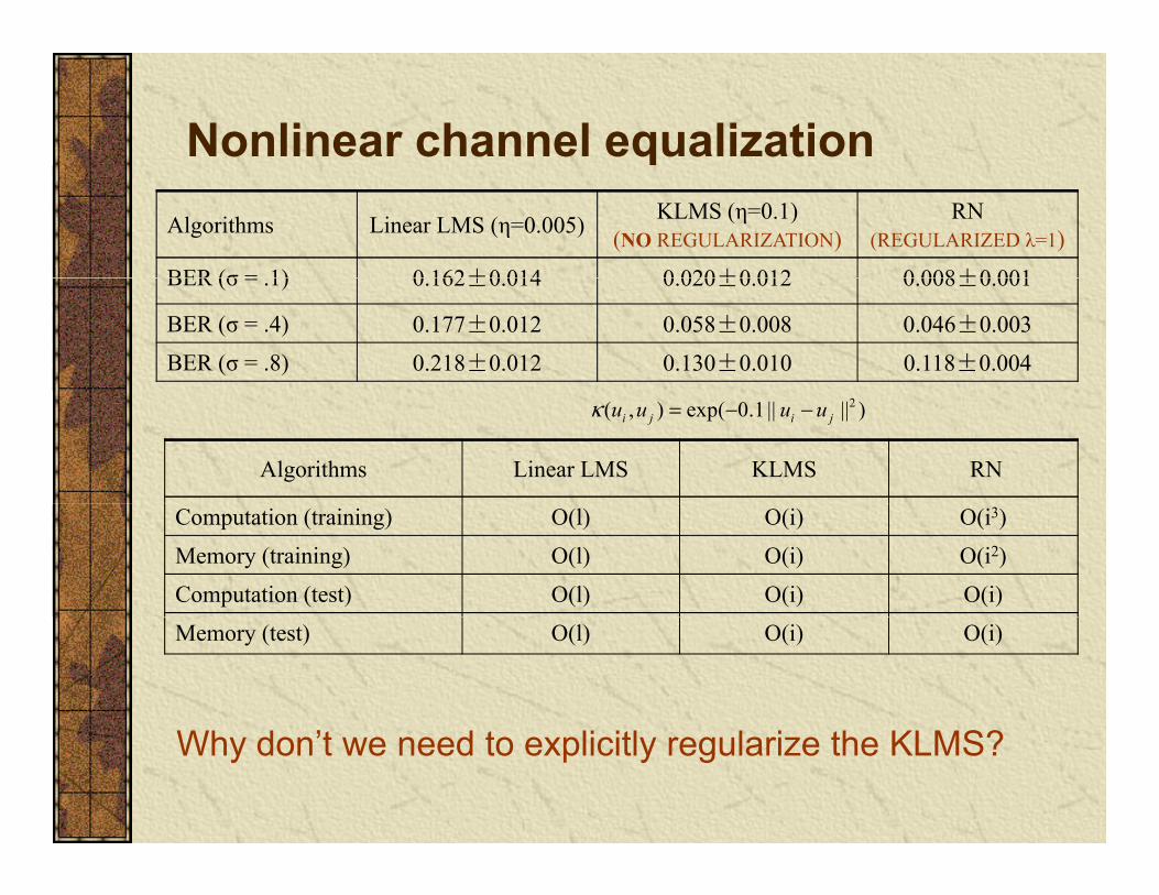
Nonlinear channel equalizationAlgorithms Linear LMS (η=0.005) KLMS (η=0.1)
(NO REGULARIZATION)RN
(REGULARIZED λ=1)
BER (σ = 1) 0 162±0 014 0 020±0 012 0 008±0 001BER (σ = .1) 0.162±0.014 0.020±0.012 0.008±0.001
BER (σ = .4) 0.177±0.012 0.058±0.008 0.046±0.003BER (σ = .8) 0.218±0.012 0.130±0.010 0.118±0.004
Algorithms Linear LMS KLMS RN
2( , ) exp( 0.1 || || )i j i ju u u uκ = − −
Computation (training) O(l) O(i) O(i3)
Memory (training) O(l) O(i) O(i2)
Computation (test) O(l) O(i) O(i)
Memory (test) O(l) O(i) O(i)
S?Why don’t we need to explicitly regularize the KLMS?

Self-regularization property of KLMSg p p y
Assume the data model then for any unknown vector the following inequality holds
( ) ( ) ( )oid i v iϕ= Ω +
0Ωunknown vector the following inequality holds2
111 2 2
| ( ) ( ) |1, 1,2,...,
|| || | ( ) |
i
jio
e j v jfor all i N
jη=
−−
−< =
Ω +
Ω
As long as the matrix is positive definite. SoH∞ robustness
1|| || | ( ) |o
jv jη
=Ω +
})()({ 1 TiiI ϕϕη −−
H robustness
And is upper bounded
2 1 2 2|| || || || 2 || ||oe vη−< Ω +
)(nΩAnd is upper bounded
Th l ti f KLMS i l b d d i
2 2 21|| || (|| || 2 || || )o
N vσ η ηΩ < Ω + σ1 is the largest eigenvalue of Gφ
)(nΩ
The solution norm of KLMS is always upper bounded i.e. the algorithm is well posed in the sense of Hadamard.
Liu W., Pokarel P., Principe J., “The Kernel LMS Algorithm”, IEEE Trans. Signal Processing, Vol 56, # 2, 543 – 554, 2008.

Regularization Techniques
Learning from finite data is ill-posed and a priori information to enforce Smoothness is needed.information to enforce Smoothness is needed.The key is to constrain the solution norm
In Least Squares constraining the norm yieldsN
Norm constraint
In Bayesian modeling, the norm is the prior. (Gaussian process)
2 2
1
1( ) ( ( ) ) , subject to || ||N
Ti
iJ d i C
Nϕ
=
Ω = −Ω Ω <y g p ( p )
In statistical learning theory the norm is associated with the
2 2
1
1( ) ( ( ) ) || ||N
Ti
iJ d i
Nϕ λ
=
Ω = −Ω + ΩGaussian
distributed prior
In statistical learning theory, the norm is associated with the model capacity and hence the confidence of uniform convergence! (VC dimension and structural risk minimization)

Tikhonov RegularizationgIn numerical analysis the method is to constrain the condition number of the solution matrix (or its eigenvalues)
1 2{ , ,..., }rS diag s s s=Singular value
The singular value decomposition of Φ can be written
TQS
PΦ
=
000
g
The pseudo inverse to estimate Ω in is
which can be still ill posed (very small sr) Tikhonov regularized the
00)()()( 0 iiid T νϕ +Ω=
dQP TrPI ssdiag ]0....0,,...,[ 11
1−−=Ω
s s
which can be still ill-posed (very small sr). Tikhonov regularized the least square solution to penalize the solution norm to yield
2d Ω+Ω−=Ω λTJ Φ)(1
2 21
( ,..., ,0,...,0) Tr
r
s sPdiag Q d
s sλ λΩ =
+ +Notice that if λ = 0, when sr is very small, sr/(sr
2+ λ) = 1/sr → ∞., r y , r ( r ) r
However if λ > 0, when sr is very small, sr/(sr2+ λ) = sr/ λ → 0.

Tikhonov and KLMSFor finite data and using small stepsize theory:Denote T( ) mu Rϕ ϕ= ∈ 1 N
TDenote
Assume the correlation matrix is singular, and0≥ ≥
TxR P P= Λ( )i iu Rϕ ϕ= ∈
1
1 Ti i
i
RNϕ ϕ ϕ
=
=
From LMS it is known that 1 1... ... 0k k mς ς ς ς+≥ ≥ > = = =
)0()1()]([ ni
nn iE εηςε −=
Define so=ΩΩ m Pii 0 )()( ε
)2
)0(()1(2
])([ min22min2
nn
in
nn
JJiEης
ηεηςης
ηε−
−−+−
=
Define so
d
==Ω−Ω
n nn Pii1
)()( ε
jj
M
j
ijjj
M
j
ijiE PP 0
11
0 ])1(1[)0()1()]([ Ω−−=−+Ω=Ω ==
ηςεης 0)0(0)0( jj Ω−==Ω ε
and
Liu W., Pokarel P., Principe J., “The Kernel LMS Algorithm”, IEEE Trans. Signal Processing, Vol 56, # 2, 543 – 554, 2008.
20
1
202 )()]([ Ω=Ω≤Ω =
M
jjiE max/1 ςη ≤

Tikhonov and KLMS
In the worst case, substitute the optimal weight by the pseudo inverse dQP T
ri
ri ssdiagiE ]0....0,))1(1(,...,))1(1[()]([ 11
11−− −−−−=Ω ηςης
Regularization function for finite N in KLMS 2 1[1 (1 / ) ]N
n ns N sη −− − ⋅No regularizationTikhonov
2 2 1λ
1ns −
PCA
2 2 1[ /( )]n n ns s sλ −+ ⋅
1 if ths s− >0.8
1
onif th0 if th
n n
n
s ss
> ≤
0.2
0.4
0.6
reg-
func
tioKLMSThe stepsize and N control the reg-function in
0 0.5 1 1.5 2
0
singular value
TikhonovTruncated SVD
KLMS.
Liu W., Principe J. The Well-posedness Analysis of the Kernel Adaline, Proc WCCI, Hong-Kong, 2008
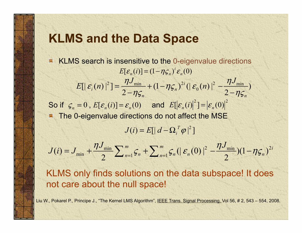
KLMS and the Data SpacepKLMS search is insensitive to the 0-eigenvalue directions
)0()1()]([ iiE εηςε −= )0()1()]([ nnn iE εηςε2 2 2min min
0[| ( ) | ] (1 ) (| ( ) | )2 2
ii n
n n
J JE n n
η ηε ης εης ης
= + − −− −
22 )()(So if , and The 0-eigenvalue directions do not affect the MSE
2( ) [| | ]TJ i E d ϕ= −Ω
0nς = )0()]([ nn iE εε = 22 )0(])([ nn iE εε =
2 2min minmin 1 1
( ) (| (0) | )(1 )2 2
m m in n n nn n
J JJ i J
η ης ς ε ης= =
= + + − −
( ) [| | ]iJ i E d ϕ= Ω
KLMS only finds solutions on the data subspace! It does not care about the null space!
Liu W., Pokarel P., Principe J., “The Kernel LMS Algorithm”, IEEE Trans. Signal Processing, Vol 56, # 2, 543 – 554, 2008.

Energy Conservation Relation
Energy conservation in RKHS
The fundamental energy conservation relation holds in RKHS!
Energy conservation in RKHS
( ) ( )222 2 ( )( )( ) ( 1)
( ), ( ) ( ), ( )pa e ie ii i
i i i iκ κ+ = − + Ω Ω
u u u uF F
Upper bound on step size for mean square convergence
( ) ( )( ), ( ) ( ), ( )
2*2E Ω
F
0.012
St d t t f
2* 2vE
ησ
≤ + Ω
F
F0.006
0.008
0.01
EM
SE
Steady-state mean square performance2
2lim ( )2
vai
E e i ηση→∞
= 0.002
0.004
simulationtheory
Chen B., Zhao S., Zhu P., Principe J. Mean Square Convergence Analysis of the Kernel Least Mean Square Algorithm, IEEE Trans. Signal Processing
2i η→∞ −0.2 0.4 0.6 0.8 1
0
stepsize η

Effects of Kernel Size
7
8
x 10-3
simulationtheory
0.6
0.7
0.8
σ = 0.2σ = 1.0σ = 20
4
5
6
EM
SE0.4
0.5
EM
SE
1
2
3
E
0.1
0.2
0.3
0.5 1 1.5 20
1
kernel size σ
0 200 400 600 800 10000
iteration
Kernel size affects the convergence speed! (How to choose a suitable kernel size is still an open problem)
H i d ff h fi l i dj ! ( i lHowever, it does not affect the final misadjustment! (universal approximation with infinite samples)

Part 3: Affine projection algorithms in p j gkernel space
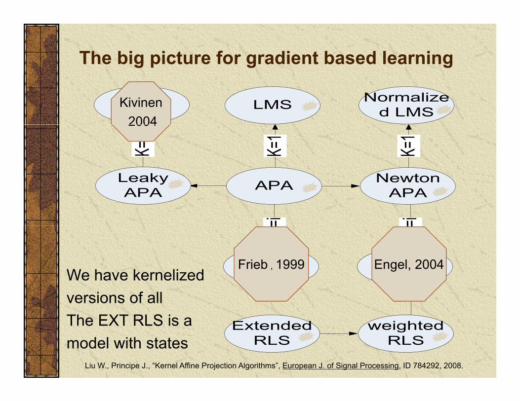
The big picture for gradient based learning
Kivinen20042004
Frieb , 1999 Engel, 2004We have kernelizedWe have kernelized versions of allThe EXT RLS is amodel with states
Liu W., Principe J., “Kernel Affine Projection Algorithms”, European J. of Signal Processing, ID 784292, 2008.

Affine projection algorithmsp j gSolve which yields 2
)(min uww T
wdEJ −= du
-1u rRw =0
There are several ways to approximate this solution iteratively using
Gradient Descent Method
Newton’s recursion )]1([)1()()0( −+−= iii wR-rwww uduη
)]1([)()1()()0( 1 −++−= − iii wR-rIRwww dεη
LMS uses a stochastic gradient that approximates
)]1([)()1()()0( ++ iii wRrIRwww uduu εη
)()(ˆ)()(ˆ iidii T uruuR ==
Affine projection algorithms (APA) utilize better approximationsTherefore APA is a family of online gradient based algorithms of
)()()()( iidii uruuR duu ==
y g gintermediate complexity between the LMS and RLS.

Affine projection algorithmsp j gAPA are of the general form
TidKidiiKii )]()1([)()]()1([)( +−=+−= duuU LxK idKidiiKii )](),...,1([)()](),...,1([)( +−=+−= duuU
)()(1ˆ)()(1ˆ iiK
iiK
T dUrUUR duu ==
Gradient
KK
)]1()()()()1()()0( −+−= iiiiii T wU-[dUwww η
Newton
Notice that)]1()()()[())()(()1()( 1 −++−= − iiiiiiii TT wU-dUIUUww εη
Notice that
So11 ))()()(()())()(( −− +=+ IUUUUIUU εε iiiiii TT
)]1()()([])()()[()1()( 1 −++−= − iiiiiiii TT wU-dIUUUww εη

Affine projection algorithmsp j gIf a regularized cost function is preferred
22)(i λTdEJ
The gradient method becomes
)(min wuww λ+−= T
wdEJ
g
)]1()()()()1()1()()0( −+−−= iiiiii T wU-[dUwww ηηλ
Newton
Or)()())()(()1()1()( 1 iiiiii T dUIUUww −++−−= εηηλ
Or
)(])()()[()1()1()( 1 iiiiii T dIUUUww −++−−= εηηλ

Kernel Affine Projection Algorithmsj g
KAPA 1 2 use the least squares cost while KAPA 3 4 are regularized
Ω≡wQ(i)
KAPA 1,2 use the least squares cost, while KAPA 3,4 are regularizedKAPA 1,3 use gradient descent and KAPA 2,4 use Newton updateNote that KAPA 4 does not require the calculation of the error by
iti th ith th t i i i l d i threwriting the error with the matrix inversion lemma and using the kernel trick
Note that one does not have access to the weights, so need recursion i KLMSas in KLMS.
Care must be taken to minimize computations.

KAPA-1
( )mi i
mi i
c ua e iη←←
1 1
( )( 1)
mi i
mi mi ia a e iη
η− −← + −
1 1 ( 1)mi K mi K ia a e i Kη− + − +← + − +1
( ) ( ) ( )i
i i F j jf u u a u uϕ κ= Ω =
mi
1( ) , ( ) ( , )i i F j j
jf u u a u uϕ κ
=
Ω

KAPA-1
) )(();(1 jjieffi
ii u+= κη ),.)(();(11
1 jjieffKj
ii u+ +−=
− κη
1,....,11);()1()();()(
iKjjieiiiiei
jj
i
aaa
−+−=+−==
ηη
)}()1({)(
,...,1)1()(
1,....,11);()1()(
iiCiC
Kijii
iKjjieii
jj
jj
aa
aa
−=−=
++η
)}(),1({)( iiCiC u−=

Error reusing to save computationg p
For KAPA-1, KAPA-2, and KAPA-3T l l t K i i (k l l ti )To calculate K errors is expensive (kernel evaluations)
1( ) ( ) , ( 1 )Ti k ie k d k i K k iϕ −= − Ω − + ≤ ≤
K times computations? No, save previous errors and use them
( ) ( ) ( ) ( )T Te k d k d k eϕ ϕ η= − Ω = − Ω + Φ1 1
1
( ) ( ) ( ) ( )
( ( ) )
( )
i k i k i i iT T
k i k i iT
e k d k d k e
d k e
k
ϕ ϕ ηϕ ηϕ
+ −
−
= Ω = Ω + Φ
= − Ω + Φ
Φ Still needs ( 1)e i +( )
( ) ( ) .
Ti k i i
iT
i i k j
e k e
e k e j
ηϕ
η ϕ ϕ
= + Φ
= +
Still needs which requires i kernel evals,
So O(i+K2)
( 1)ie i +
1( ) ( ) .i i k j
j i Ke k e jη ϕ ϕ
= − +
+

KAPA-4
KAPA-4: Smoothed Newton’s method.
1 1[ , ,..., ]
[ ( ), ( 1),..., ( 1)]i i i i K
Tid d i d i d i K
ϕ ϕ ϕ− − +Φ =
= − − +There is no need to compute the error
)(])()()[()1()1()( 1 iiiiii T dIww −+ΦΦΦ+−−= ληηλ
The topology can still be put in the same RBF framework. Efficient ways to compute the inverse are necessary The slidingEfficient ways to compute the inverse are necessary. The sliding window computation yields a complexity of O(K2)

KAPA-4
)(~)( ikidika ==η
11)1()1()(11)(~)1()1()(
KikiiikKikdii
kk
kk
aaaa
+−≤≤−−=−≤≤+−+−−=
ηηη
)())(()(~11)1()1()(
1 iii
Kikii kk
dIGd
aa−+=
+≤≤
λη
How to invert the K-by-K matrix and avoid O(K3)?( )Ti iIε + Φ Φ

Sliding window Gram matrix inversion
Ti i iGr = Φ Φ
g
1 1[ , ,..., ]i i i i Kϕ ϕ ϕ− − +Φ =T
ia b
Gr Ib D
λ
+ =
1i T
D hGr I
h gλ+
+ =
Sliding window
b D
1 /TD H ff e− = −
g
1( )T
ie f
Gr Iλ − + =
Assume known
1
( )i f H
1 1( )Ts g h D h− −= −2
Schur complement of D
1 1 1 11
1 1
( )( ) ( )( )
T
i T
D D h D h s D h sGr Iλ
− − − −−
+
+ −+ =
( )s g h D h
3
Sc u co p e e t o
1 1( )( )i TD h s s+ − −
Complexity is K2
Relations to other methods

Recursive Least-Squaresq
The RLS algorithm estimates a weight vector w(i-1) by minimizing the cost functiong
The solution becomes
21
1)()(
−
=
−i
j
T
wjjdnim wu
e so ut o beco es
And can be recursively computed as
)1()1())1()1(()1( 1 −−−−=− − iiiii T dUUUw
)]1()()([)()1()(1
)()1()1()( −−−+
−+−= iiidiii
iiii TT wu
uPuuPww
1TWhere . Start with zero weights and
)()()1()()()1()(1)( +−=−+= ieiiiiiiir T kwwuPu
1))()(()( −= Tiii UUP I1)0( −= λP
)1()()()()]()()()1([)()(/)()1()(
−−=−−=−=
iiidieiriiiiiriii
T
T
wukkPPuPk

Kernel Recursive Least-SquaresqThe KRLS algorithm estimates a weight function w(i) by minimizing
221
)()( ww λϕ +−−i
T jjdnim
The solution in RKHS becomes 1
)()( ϕ=jw
jj
[ ] )()()()()()()( 1 iiiiiIii T adw Φ=ΦΦ+Φ= −λ )()()( iii dQa =can be computed recursively as
[ ] )()()()()()()()(i-1Q
)()1()()())()(
)()1()(
1
iiiiii
iii T
TTϕ
λ−Φ=
−=
−
hh
hQQ-1
From this we can also recursively compute Q(i) )()1()()()()()()1(
)()( 1 iiiiiiiriiri
T hQzzzzQQ
−=
−+−
= −
)())()( iii TT ϕϕλ
+h
And compose back a(i) recursively )()())(),(()(1)(
)()(iiiiiri
iri TT hzuuz-Q
−+=
=κλ
)1()()()()()()()(
)(1
−−=
−=
−
iiidieieirii
i T ahza
a
with initial conditions
)1()()()()()(
)( 1 =
=
−iiidie
ieiri aha
[ ] )1()1()1(,))(),(()1( 1 dii T QauuQ =+= −κλ

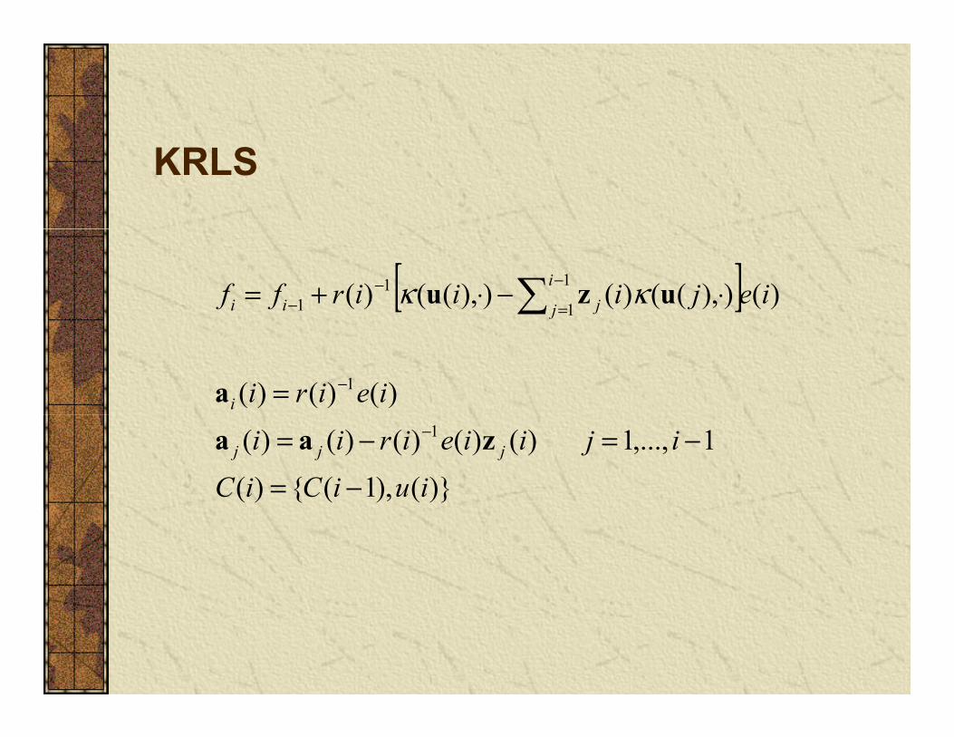
KRLS
)()( 1 ieira
uc
mi
imi−←
←
1
)()()( 1 iieiraa jjmijmi z−−− −←
1
2
1
2
mi-1
mimi-1
mi )),(()()(1
uuau jifi
ji κ
=
=1j=
Engel Y., Mannor S., Meir R. “The kernel recursive least square algorithm”, IEEE Trans. SignalProcessing, 52 (8), 2275-2285, 2004.
KRLS
[ ] )()),(()()),(()( 1
11
1 iejiiirff i
j jii ⋅−⋅+= −
=−
− uzu κκ
)()()( 1 ieirii = −a
)}(),1({)(
1,...,1)()()()()( 1
iuiCiC
ijiieirii jjj
−=
−=−= − zaa

Regularizationg
The well posedness discussion for the KLMS hold forThe well-posedness discussion for the KLMS hold for any other gradient decent methods like KAPA-1 and KAPA-3If Newton method is used, additional regularization is needed to invert the Hessian matrix like in KAPA-2 and normalized KLMSand normalized KLMSRecursive least squares embed the regularization in the initialization
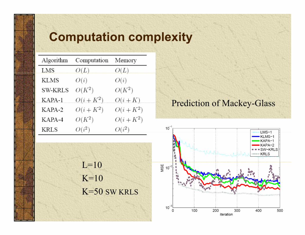
Computation complexityy
Prediction of Mackey GlassPrediction of Mackey-Glass
L 10L=10K=10K=50 SW KRLSK=50 SW KRLS

Simulation 1: noise cancellationn(i) ~ uniform [-0.5, 05]
( ) ( ) 0.2 ( 1) ( 1) ( 1) 0.1 ( 1) 0.4 ( 2)u i n i u i u i n i n i u i= − − − − − + − + −( ( ), ( 1), ( 1), ( 2))H n i n i u i u i= − − −

Simulation 1: Noise Cancellation
2( ( ) ( )) exp( || ( ) ( ) || )u i u j u i u jκ =( ( ), ( )) exp( || ( ) ( ) || )u i u j u i u jκ = − −
K=10

Simulation 1:Noise Cancellation
0 50
0.5
Noisy Observation
2500 2520 2540 2560 2580 2600-1
-0.5
00.5
NLMS
2500 2520 2540 2560 2580 2600
-0.50
0.5
KLMS 1litut
e
2500 2520 2540 2560 2580 2600-0.5
00.5
KLMS-1
0 5
Am
pl
2500 2520 2540 2560 2580 2600-0.5
00.5
KAPA-2
2500 2520 2540 2560 2580 2600i

Simulation-2: nonlinear channel equalization
10.5t t tz s s −= + 20.9t t tr z z nσ= − +
K=100 1σ=0.1

Simulation-2: nonlinear channel equalization
Nonlinearity changed (inverted signs)

Gaussian Processes A Gaussian process is a stochastic process (a family of random variables) where all the pairwise correlations are Gaussian distributed The family however is not necessarily over time (as indistributed. The family however is not necessarily over time (as in time series). For instance in regression, if we denote the output of a learning system by y(i) given the input u(i) for every i, the conditional probability
Where σ is the observation Gaussian noise and G(i) is the Gram t i
))(,0()(),...,1(|)(),...1(( 2 iGInuunyyp n +Ν= σ
matrix
=
))(),1(())1(),1(()(
iiG
uuuu κκ
and κ is the covariance function (symmetric and positive definite). Just lik th G i k l d i KLMS
))(),(())1(),(( iii uuuu κκ
like the Gaussian kernel used in KLMS. Gaussian processes can be used with advantage in Bayesian
inference.
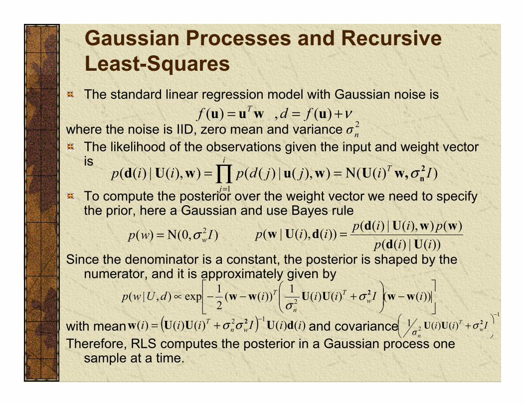
Gaussian Processes and Recursive Least-SquaresqThe standard linear regression model with Gaussian noise is
h th i i IID d iν+== )(,)( u wuu fdf T
2where the noise is IID, zero mean and variance The likelihood of the observations given the input and weight vector is
))(()),(|)(()),(|)(( Iijjdpiip Ti
2w,UwuwUd σΝ==∏
2nσ
To compute the posterior over the weight vector we need to specify the prior, here a Gaussian and use Bayes rule
2
))(()),(|)(()),(|)((1
Iijjdpiipj
nw,UwuwUd σΝ∏=
)())(|)(( piip wwUd
Since the denominator is a constant, the posterior is shaped by the numerator, and it is approximately given by
),0()( 2 Iwp wσΝ=))(|)((
)()),(|)(())(),(|(iip
piipiipUd
wwUddUw =
, pp y g y
with mean and covariance
−
+−−∝ ))(()()(1))((
21exp),|( 2 iIiiidUwp w
T
n
T wwUUww 2σσ
( ) )()()()()( 12 iiIiii wnT dUUUw 2 −+= σσ
1
2 )()(1−
+ Iii w
T 2UU σwith mean and covarianceTherefore, RLS computes the posterior in a Gaussian process one
sample at a time.
( ) )()()()()( wn 2 )()( σ w
n

KRLS and Nonlinear Regression
It easy to demonstrate that KRLS does in fact estimate online nonlinear regression with a Gaussian noise model i.e.
νϕ +== )(()( uwu)u fdf T
where the noise is IID, zero mean and variance By a similar derivation we can say that the mean and variance are
νϕ +== )(,()( u wu)u fdf2nσ
( ) 11−
Although the weight function is not accessible we can create predictions at any point in the space by the KRLS as
( ) )()()()()( 12 iiIiii wnT dw 2 Φ+ΦΦ= −σσ 2 )()(1
+ΦΦ Iiiσ w
T
n
2σ
predictions at any point in the space by the KRLS as
with variance ( ) )()()()()()]([ˆ 12 iIiiifE wn
TT duu 2 −+ΦΦΦ= σσϕ
( ) 12222 2 TTTT −( ) )()()()()()()()())(( 12222 uuuuu 2 ϕσσϕσϕϕσσ Twn
TTw
Tw iIiiif Φ+ΦΦΦ−=
Part 4: Extended Recursive least squares in kernel space

Extended Recursive Least-Squaresq
STATE modelnxFx +=
Start withii
Tii
iiii
vxUd
nxFx
+=
+=+1
Start with
Special cases
10| 1 0| 1,w P −− − = Π
Notations:p• Tracking model (F is a time varying scalar)
• Exponentially weighted RLS1 , ( ) ( )T
i i i i ix x n d i u x v iα+ = + = +xi state vector at
time i
wi|i-1 state estimate • Exponentially weighted RLS
• standard RLS1 , ( ) ( )T
i i i ix x d i u x v iα+ = = +
i|i 1at time i using data up to i-1
1 , ( ) ( )Ti i i ix x d i u x v i+ = = +
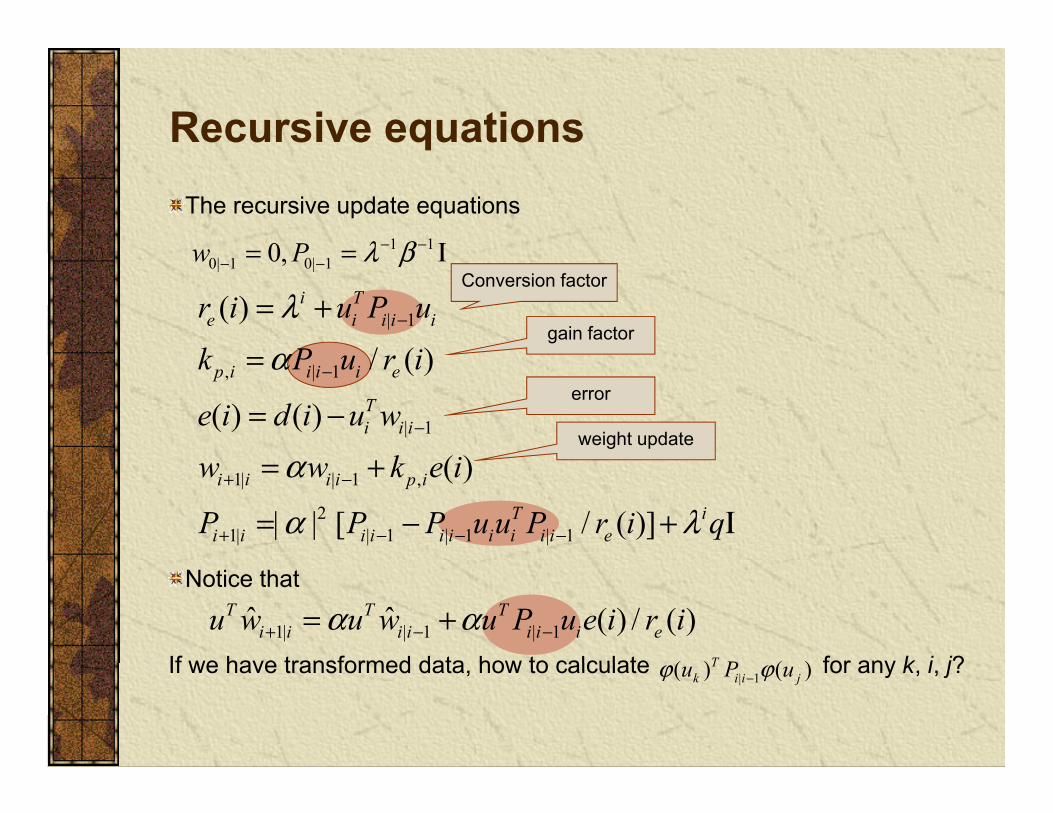
Recursive equationsThe recursive update equations
q
1 10w P λ β− −= = Ι0| 1 0| 10,w P λ β− −= = ΙConversion factor
gain factor| 1( )
/ ( )
i Te i i i ir i u P u
k P u r i
λα
−= +
weight update
error, | 1
| 1
/ ( )
( ) ( )( )
p i i i i e
Ti i i
k P u r i
e i d i u wk i
α −
−
=
= −
1| | 1 ,
21| | 1 | 1 | 1
( )
| | [ / ( )]i i i i p i
T ii i i i i i i i i i e
w w k e i
P P P u u P r i q
α
α λ+ −
+ − − −
= +
= − + Ι
Notice that
If we have transformed data how to calculate for any k i j?( ) ( )T P
1| | 1 | 1ˆ ˆ ( ) / ( )T T Ti i i i i i i eu w u w u P u e i r iα α+ − −= +
If we have transformed data, how to calculate for any k, i, j?| 1( ) ( )T
k i i ju P uϕ ϕ−

New Extended Recursive Least-squares
Theorem 1:
q
| 1 1 1 1 1,Tj j j j j jP H Q H jρ= Ι − ∀Theorem 1:
where is a scalar, and is a jxj matrix, for all j.Proof:
| 1 1 1 1 1,j j j j j jQ jρ− − − − −
1jρ − 1 0 1[ ,..., ]Tj jH u u− −= 1jQ −
1 1 1 1 0P Qλ β ρ λ β− − − −= Ι = =0| 1 1 1, , 0P Qλ β ρ λ β− − −= Ι = =
| 1 | 121| | 1| | [ ]
( )
Ti i i i i i i
i i i i
P u u PP P q
iα λ− −
+ −= − + ΙBy mathematical
induction!| |
21 1 1 1
1 1 1 1 1 1 1 1
( )
| | [
( ) ( )]
eT
i i i iT T T
ii i i i i i i i i i
r i
H Q H
H Q H u u H Q H
α ρρ ρ λ
− − − −= − −
− −Ι1 1 1 1 1 1 1 1
1 11 1, 1, 1 1,2 2
1
( ) ( )]
( )
( ) ( )(| | ) | |
ii i i i i i i i i i
e
Ti i i i i e i i i ei T
i i
Q Qq
r i
Q f f r i f r iq H
ρ ρ λ
ρα ρ λ α
− − − − − − − −
− −− − − − −
+ Ι
+ −= + Ι− iH
1
1
(| | ) | |i ii
q Hα ρ λ αρ−−
+ Ι− 1 2 1
1, 1( ) ( )Ti i e i e
if r i r iH
ρ− −− −
Liu W., Principe J., “Extended Recursive Least Squares in RKHS”, in Proc. 1st Workshop on Cognitive Signal Processing, Santorini, Greece, 2008.

New Extended Recursive Least-squares
Theorem 2:
q
| 1 1 | 1ˆ ,Tj j j j jw H a j= ∀Theorem 2:
where and is a vector, for all j.Proof:
| 1 1 | 1,j j j j jw H a j− − − ∀
1 0 1[ ,..., ]Tj jH u u− −= | 1j ja − 1j ×
ˆ 0 0w a= =0| 1 0| 10, 0w a− −= =
1| | 1 ,ˆ ˆ ( )
( ) / ( )i i i i p i
T
w w k e i
H a P u e i r i
α
α α+ −= +
+
By mathematical induction again!
1 | 1 | 1
1 | 1 1 1 1 1
( ) / ( )
( ) ( ) / ( )
( ) / ( ) ( ) / ( )
i i i i i i e
T Ti i i i i i i i e
T T
H a P u e i r i
H a H Q H u e i r i
H i i H f i i
α α
α α ρ− − −
− − − − − −
= +
= + Ι −
+1 | 1 1 1 1,
1| 1 1,
( ) / ( ) ( ) / ( )
( ) ( )( )
T Ti i i i i e i i i e
T i i i i ei
H a u e i r i H f e i r i
a f e i r iH
e i r
α αρ α
α ααρ
− − − − −
−− −
= + −
−= 1( )i−
1 ( )i e i rαρ − ( )e i

Extended RLS New Equations 1 1
0| 1 0| 10,w P λ β− −− −= = Ι
1 10| 1 1 10, , 0a Qρ λ β− −− − −= = =
T T
T
1, 1
1, 1 1,
( )
T Ti i i i
i i i i i
i T T
k u Hf Q k
k fλ
− −
− − −
==
| 1
, | 1
( )
/ ( )
i Te i i i i
p i i i i e
r i u P u
k P u r i
λα
−
−
= +
=1 1, 1,
1, | 1
1
( )
( ) ( )
i T Te i i i i i i i
Ti i i i
r i u u k f
e i d i k a
λ ρ − − −
− −
= + −
= −
| 1
1| | 1 ,
( ) ( )
( )
Ti i i
i i i i p i
e i d i u w
w w k e iα−
+ −
= −
= +
1| 1 1,
1| 11
2
( ) ( )( ) ( )
| |
i i i i ei i
i e
i
a f r i e ia
r i e iα
ρ
λ
−− −
+ −−
−=
21| | 1
| 1 | 1
| | [
/ ( )]i i i i
T ii i i i i i e
P P
P u u P r i q
α
λ+ −
− −
= −
+ Ι
21| | i
i i qρ α ρ λ−= +
1 11 1, 1, 1 1,2 ( ) ( )
| |T
i i i i i e i i i ei
Q f f r i f r iQ
ρα
− −− − − − −+ −
= | |1 2 1
1 1, 1( ) ( )| |
Ti i i e i e
i f r i r iQ
ρ ρα
− −− − −−

An important theoremp
Assume a generalAssume a general nonlinear state-space model
))(()1( isgis =+ ))(())1(( ixix =+ sAs
)())(),(()( iiihid ν+= su )())(())(()( iixiid T νϕ += su
)()()( uuuu ′=′ κϕϕ T ),()()( uuuu = κϕϕ
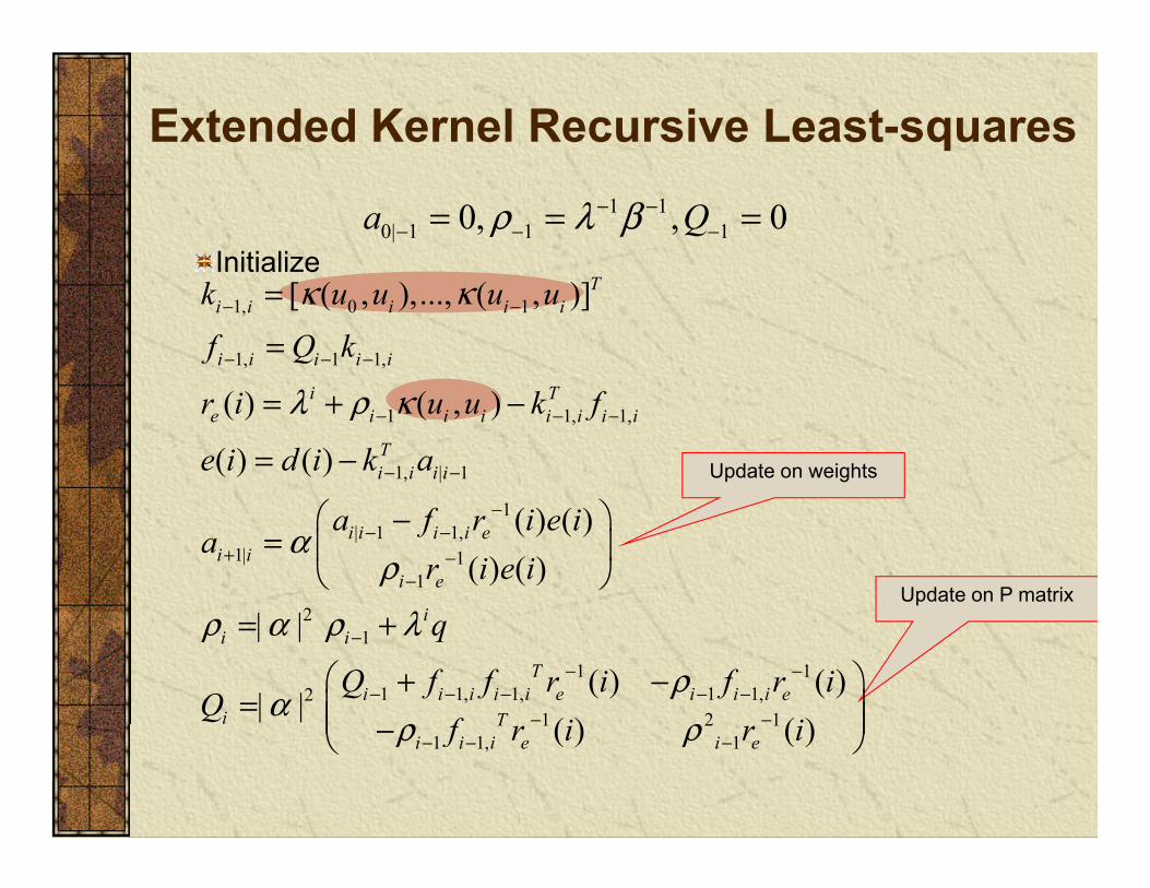
Extended Kernel Recursive Least-squares
Initialize
1 10| 1 1 10, , 0a Qρ λ β− −− − −= = =
1, 0 1
1, 1 1,
[ ( , ),..., ( , )]Ti i i i i
i i i i i
i T
k u u u uf Q k
κ κ− −
− − −
==
Update on weights
1 1, 1,
1, | 1
( ) ( , )
( ) ( )
i Te i i i i i i i
Ti i i i
r i u u k f
e i d i k a
λ ρ κ− − −
− −
= + −
= −
Update on P matrix
1| 1 1,
1| 11
2
( ) ( )( ) ( )
i i i i ei i
i e
i
a f r i e ia
r i e iα
ρ
λ
−− −
+ −−
−=
2
1
1 1, 1,2
| |
| |
ii i
i i i i ii
q
Q f fQ
ρ α ρ λ
α
−
− − −
= +
+=
1 11 1,
1 2 1
( ) ( )( ) ( )
Te i i i e
T
r i f r if i i
ρρ ρ
− −− −
− −
−
1 2 11 1, 1( ) ( )T
i i i e i ef r i r iρ ρ− − − −
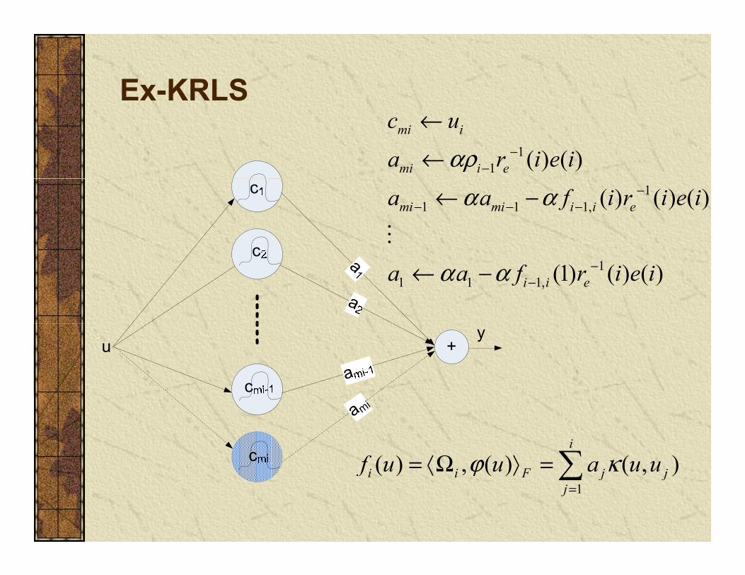
Ex-KRLS
11 ( ) ( )
mi i
mi i e
c u
a r i e iαρ −−
←
←1
1 1 1, ( ) ( ) ( )mi mi i i ea a f i r i e iα α −− − −← −
1 11 1 1, (1) ( ) ( )i i ea a f r i e iα α −
−← −
( ) ( ) ( )i
i i F j jf u u a u uϕ κ= Ω =
mi
1( ) , ( ) ( , )i i F j j
jf u u a u uϕ κ
=
Ω

Simulation-3: Lorenz time series prediction

Simulation-3: Lorenz time series prediction (10 steps)

Simulation 4: Rayleigh channel trackingy g g
1 0001,000symbols
fD=100Hz, t=8x10⁻⁵s σ=0.005

Rayleigh channel trackingy g g
Al i h MSE (dB) (noise variance MSE (dB) (noise i 0 01 d fAlgorithms MSE (dB) (noise variance
0.001 and fD = 50 Hz ) variance 0.01 and fD = 200 Hz )
ε-NLMS -13.51 -9.39RLS -14.25 -9.55Extended RLS -14.26 -10.01Kernel RLS -20.36 -12.74Kernel extended RLS -20.69 -13.85
2( ) ( 0 1 || || )2( , ) exp( 0.1 || || )i j i ju u u uκ = − −

Computation complexityAl ith Linear KLMS KAPA KRLSAlgorithms LMS KLMS KAPA ex-KRLS
Computation (training) O(l) O(i) O(i+K2) O(i2)
Memory (training) O(l) O(i) O(i+K) O(i2)
Computation (test) O(l) O(i) O(i) O(i)
Memory (test) O(l) O(i) O(i) O(i)
At time or iteration i

Part 5: Active learning in kernel adaptive filtering and Adaptive kernel p g psize

Active data selection
Why?Why?Kernel trick may seem a “free lunch”!The price we pay is memory and pointwise evaluations of the functionthe function.Generalization (Occam’s razor)
B t b ki li iBut remember we are working on an on-line scenario, so most of the methods out there need to be modified.

Active data selection
The goal is to build a constant length (fixed budget)The goal is to build a constant length (fixed budget) filter in RKHS. There are two complementary methods of achieving this goal:
Discard unimportant centers (pruning)Accept only some of the new centers (sparsification)
Apart from heuristics, in either case a methodology to evaluate the importance of the centers for the overall pnonlinear function approximation is needed.Another requirement is that this evaluation should be no more expensive computationally than the filterno more expensive computationally than the filter adaptation.

Previous Approaches – Sparsificationpp pNovelty condition (Platt, 1991)
• Compute the distance to the current dictionaryCompute the distance to the current dictionary
• If it is less than a threshold δ1 discardIf the prediction error
jiDcciudis
j
−+=∈
)1(min)(
• If the prediction error
• Is larger than another threshold δ2 include new center. )()1()1()1( iiidie TΩ+−+=+ ϕ
Approximate Linear dependency (Engel, 2004)• If the new input is a linear combination of the previous
centers discardcenters discard
which is the Schur Complement of Gram matrix and fits KAPA 2 d 4 ll P bl i t ti l l it
∈−+=
)(2 )()1((miniDc jj
jcbiudis ϕϕ
and 4 very well. Problem is computational complexity

Previous Approaches – Pruningpp gSliding Window (Vaerenbergh, 2010)
Impose mi<B in =im
jji ciaf )()( κImpose mi<B in Create the Gram matrix of size B+1 recursively from size B
=+
)()1(
hiGiG
=j
jji ciaf1
,.)()( κ
[ ]TBBB cccch ),(),...,,( 111 ++= κκ
=+
++ ),()1(
11 BBT cch
iGκ
hzccrhiQziGIiQ TBB −+==+= ++
− ),()())(()( 111 κλλ
+iQ T //)(
Downsize: reorder centers and include last (see KAPA2)
−−+
=+rrzrzrzziQ
iQ T
T
/1///)(
)1(
See also the Forgetron and the Projectron that provide error bounds for the approximation
=+ +=++=+−=+ B
j jjiT ciafidiQiaeffHiQ
11 ,.)()1()1()1()1(/)1( κ
error bounds for the approximation. O. Dekel, S. Shalev-Shwartz, and Y. Singer, “The Forgetron: A kernel-based perceptron on a fixed budget,” in Advancesin Neural Information Processing Systems 18. Cambridge, MA: MIT Press, 2006, pp. 1342–1372.F. Orabona, J. Keshet, and B. Caputo, “Bounded kernel-based online learning,” Journal of Machine Learning Research,vol. 10, pp. 2643–2666, 2009.

Problem statement
Th l i t ))(( iTThe learning systemAlready processed (your dictionary)
))(;( iTuy
ijdjuiD )}()({)( =
A new data pair How much new information it contains?
jjdjuiD 1)}(),({)( ==)}1(),1({ ++ idiu
How much new information it contains?Is this the right question?
OrHow much information it contains with respect to the
learning system ?))(;( iTuy

Information measure
Hartley and Shannon’s definition of informationHow much information it contains?
))1(),1((ln)1( ++−=+ idiupiI
Learning is unlike digital communications:The machine never knows the joint distribution!
When the same message is presented to a learning system information (the degree of uncertainty) changes because the system learned with the first g ypresentation! Need to bring back MEANING into information theory!
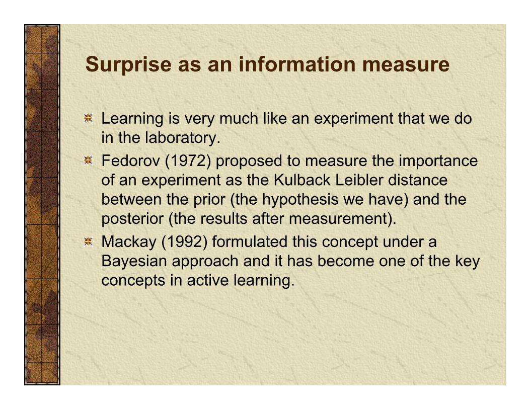
Surprise as an information measurep
Learning is very much like an experiment that we do in the laboratory. Fedorov (1972) proposed to measure the importance of an experiment as the Kulback Leibler distanceof an experiment as the Kulback Leibler distance between the prior (the hypothesis we have) and the posterior (the results after measurement).Mackay (1992) formulated this concept under a Bayesian approach and it has become one of the key concepts in active learningconcepts in active learning.

Surprise as an information measurep
))(log()( xqxIS −=
))(;( iTuy
))(|)1((ln)1())1(()( iTiupiSiuS iT +−=+=+
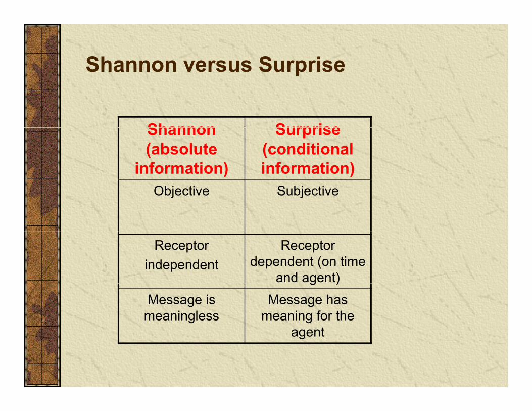
Shannon versus Surprise
Shannon SurpriseShannon (absolute
information)
Surprise (conditional information)
Objective Subjective
Receptorindependent
Receptor dependent (on time
and agent)g )Message is
meaninglessMessage has
meaning for the agentagent

Evaluation of surprisep
Gaussian process theoryGaussian process theory
))1(ˆ)1((
))](|)1(),1((ln[)1(2idid
iTidipiS
++
=++−=+ u
where
))](|)1((ln[)1(2
))1()1(()1(ln2ln 2 iTipi
ididi +−++−++++ u
σσπ
)()]([)1()1(ˆ)]),1((),...,),1(([)1(
12
1
++=+
++=+− idiiid
cicii
nT
Tm
GIh
uuh
σ
κκ
)1()]([)1())1(),1(()1(
)()]([)()(1222 +++−+++=+ − iiiiii n
Tn
n
hGIhuu σκσσ

Interpretation of surprise
ˆ))](|)1(),1((ln[)1(
2
iTidipiS =++−=+ u
))](|)1((ln[)1(2
))1(ˆ)1(()1(ln2ln 2
2
iTipi
ididi +−++−++++ u
σσπ
Prediction errorLarge error large conditional information
Prediction variance
)1(ˆ)1()1( +−+=+ ididie
)1(2 +iσPrediction varianceSmall error, large variance large SLarge error, small variance large S (abnormal)
I t di t ib ti
)1( +iσ
))(|)1(( iTip +uInput distributionRare occurrence large S
))(|)1(( iTip +u
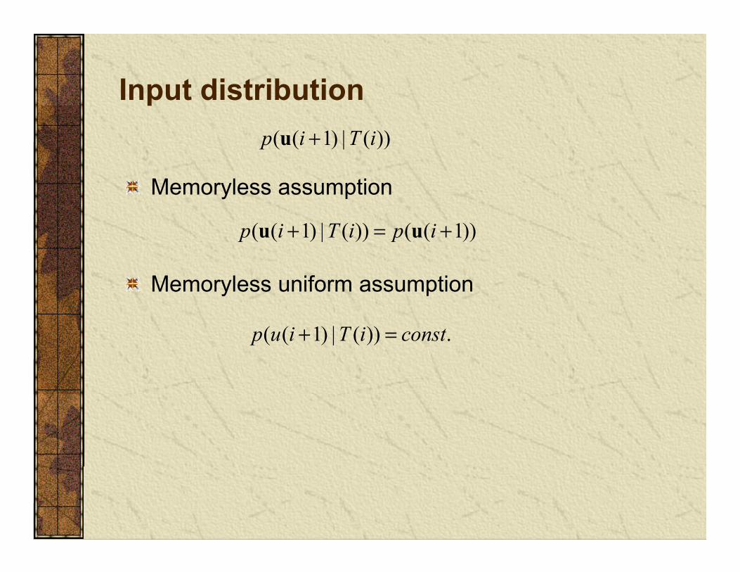
Input distributionp))(|)1(( iTip +u
Memoryless assumption
))1(())(|)1(( +=+ ipiTip uu
Memoryless uniform assumption
.))(|)1(( constiTiup =+

Unknown desired signalg
Average S over the posterior distribution of the outputAverage S over the posterior distribution of the output
))](|)1((ln[)1(ln)1( iTipiiS +−+=+ uσ
Memoryless uniform assumption
This is equivalent to approximate linear dependency!
)1(ln)1( +=+ iiS σ

Redundant, abnormal and learnable
1)1(: TiSAbnormal >+ 1
)1(
)(
TiSTL bl ≥≥ 21 )1(: TiSTLearnable ≥+≥
2)1(:Re TiSdundant <+
Still need to find a systematic way to select these thresholds which are hyperparameters.

Simulation-5: KRLS-SC nonlinear regression
Nonlinear mapping is y=-x+2x2+sin x in unit variance Gaussian noise

Simulation-5: nonlinear regression–5% most surprising data5% most surprising data

Simulation-5: nonlinear regression—redundancy removal

Simulation-5: nonlinear regressiong

Simulation-6: nonlinear regression—abnormality detection (15 outliers)
KRLS-SC

Simulation-7: Mackey-Glass time series prediction

Simulation-8: CO2 concentration forecasting

Quantized Kernel Least Mean SquareQuantized Kernel Least Mean SquareA common drawback of sparsification methods: the redundant input data are purely discarded!redundant input data are purely discarded!Actually the redundant data are very useful and can be, for example, utilized to update the coefficients of the current network although they are not sothe current network, although they are not so important for structure update (adding a new center). Quantization approach: the input space is quantized, if th t ti d i t h l d b i dthe current quantized input has already been assigned a center, we don’t need to add a new, but update the coefficient of that center with the new information!Intuitively, the coefficient update can enhance the utilization efficiency of that center, and hence may yield better accuracy and a more compact network.
Chen B., Zhao S., Zhu P., Principe J. Quantized Kernel Least Mean Square Algorithm, IEEE Trans. Neural Networks

Quantized Kernel Least Mean SquareQuantized Kernel Least Mean Square
Quantization in Input Space 0 0f =p p
[ ]( )1
1
( ) ( ) ( ( ))
( ) ( ) ,i
i i
e i d i f i
f f e i Q iη κ−
−
= − = +
u
u .
Quantization in RKHS (0) =
0Ω
[ ]( ) ( ) ( 1) ( )( ) ( 1) ( ) ( )
Te i d i i ii i e i iη
= − − = − +
ΩΩ Ω
ϕϕQ
Using the quantization method to
compress the input (or feature) space
[ ]( ) ( ) ( ) ( )η ϕ
and hence to compact the RBFstructure of the kernel adaptive filter
Quantization operator

Quantized Kernel Least Mean SquareQuantized Kernel Least Mean Square
The key problem is the vector quantization (VQ): y p q ( )Information Theory? Information Bottleneck? ……Most of the existing VQ algorithms, however, are not
it bl f li i l t ti b th d b ksuitable for online implementation because the codebook must be supplied in advance (which is usually trained on an offline data set), and the computational burden is rather heavy. A simple online VQ method:
1 Compute the distance between u(i) and C(i 1)1. Compute the distance between u(i) and C(i-1):
2. If keep the codebook unchanged, and quantize u(i) into the closest code-vector by
( )( )1 ( 1)
( ), ( 1) min ( ) ( 1)jj size idis i i i i
≤ ≤ −− = − −u u
CC C
( )( ), ( 1)dis i i ε− ≤u UC* arg min ( ) ( 1)jj i i= − −u C( ) ( 1) ( )i i e iη= − +a athe closest code vector by
3. Otherwise, update the codebook: , and quantize u(i) as itself { }( ) ( 1), ( )i i i= − uC C( )1 ( 1)
arg min ( ) ( 1)jj size i
j i i≤ ≤ −
uC
C* *( ) ( 1) ( )
j ji i e iη= +a a

Quantized Kernel Least Mean SquareQuantized Kernel Least Mean Square
Quantized Energy Conservation Relationgy
( ) ( )222 2
2 2
( )( )( ) ( 1)( ), ( ) ( ), ( )
paq
q q
e ie ii ii i i i
βκ κ+ = − + + Ω Ω
u u u uF F
A Sufficient Condition for Mean Square Convergence ( ) ( 1) ( ) 0 ( 1)TE e i i i C − >
Ω ϕ
2 2
( ) ( 1) ( ) 0 ( 1)
, 2 ( ) ( 1) ( )0 ( 2)
( )
a q
Ta q
a v
E e i i i C
i E e i i iC
E e iη
σ
> ∀ − < ≤ +
Ω
Ω
ϕ
ϕ
Steady-state Mean Square Performance
2 22max ,0 lim ( )
2 2v v
aiE e iγ γησ ξ ησ ξ
η η→∞
− + ≤ ≤ − −
2 2
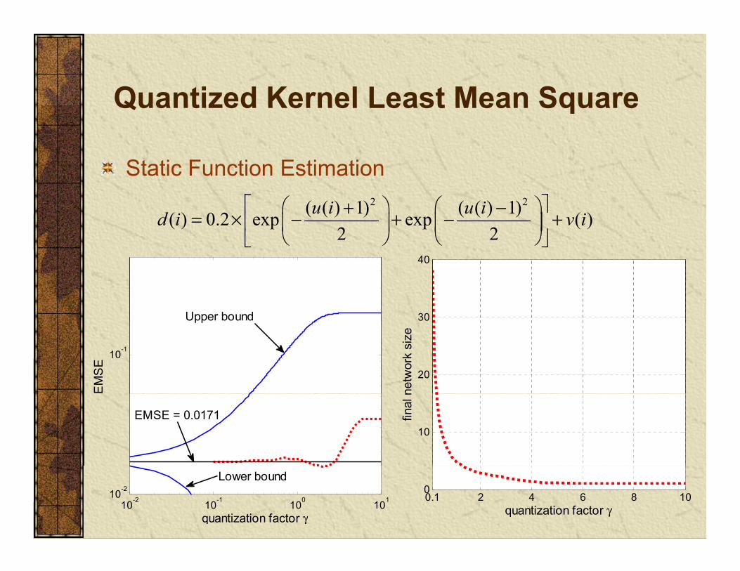
Quantized Kernel Least Mean SquareQuantized Kernel Least Mean Square
Static Function Estimation2 2( ( ) 1) ( ( ) 1)( ) 0.2 exp exp ( )
2 2u i u id i v i
+ −= × − + − +
Upper bound 30
40
10-1
EM
SE
pp
20
netw
ork
size
EMSE = 0.017110
final
n
10-2 10-1 100 10110-2
quantization factor γ
Lower bound
2 4 6 8 100.10
quantization factor γ

Quantized Kernel Least Mean SquareQuantized Kernel Least Mean Square
Short Term Lorenz Time Series Prediction
500101
QKLMS
350
400
450
e
100
SE
NC-KLMSSC-KLMS
150
200
250
300
netw
ork
siz
QKLMSNC-KLMSSC-KLMS
10-1
test
ing
MS
0 1000 2000 3000 40000
50
100
150
0 1000 2000 3000 400010-3
10-2
0 1000 2000 3000 4000iteration
0 1000 2000 3000 4000iteration

KLMS with Adaptive Kernel SizeKLMS with Adaptive Kernel Size
The kernel size controls the inner product in RKHS and pstrictly speaking when it is changed, the optimization is made on a different RKHS. So adapting the kernel size seems a daunting taskseems a daunting task.
However, since KLMS optimization is online it decouples =
=Ω=i
jjFii uujeuuf
1
),()()(,)( σκηϕσ
, p pin time, i.e. the optimization at each iteration only affects the error at that specific step. Therefore, we can in principle have contributions in different RKHS And itprinciple have contributions in different RKHS. And it turns out that we can seek the optimal kernel online.The other members of the KAPA family do not have this property!

KLMS with Adaptive Kernel SizeKLMS with Adaptive Kernel Size
We propose to change the optimization for KLMS as a p p g ptwo step process: Minimization of the error and optimization of the stepsize as
2 ( )
( )
2*
1
arg min ( , )
. . ( ) ( ), i
i
i i
i i
y f dP y
s t f f e i iσ
σ
σ
η κ+
×∈
−
= − = +
u u
u .
U Y
At iteration i, the learning starts to determine an optimal value of the kernel size σi (the old kernel sizes remain
i
unchanged), and second, adds a new center using KLMS with this new kernel size. We have shown that this converges to the optimal kernelWe have shown that this converges to the optimal kernel size.

KLMS with Adaptive Kernel SizeKLMS with Adaptive Kernel Size
The previous kernel size σi-1 can be simply optimized by p i-1 p y p yminimizing the instantaneous square error at iteration i, and a stochastic gradient algorithm can be readily derivedderived
21 1
1
( )i ii
e iσ σ μσ− −−
∂′ = − ∂∂
=iσ
( )1
1 11
1 2
2 ( ) ( ( )) ( )
2 ( ) ( ( )) ( 1) ( 1), ( ) ( )i
i ii
i i
e i f i v i
e i f i e i i i v iσ
σ μσ
σ μ η κσ −
− −−
− −
∂ = − + ∂∂ = − − − − + ∂
u
u u u
( )1
1
( )
11
( 1) ( ) ( 1), ( )i
i
c
ii
e i e i i iσ
σ
σ ρ κσ −
−
−−
∂∂= + − −∂
u u
( )2 3( 1) ( ) ( 1) ( ) ( 1) ( )i i i i i i+
We proved that this iteration converges to the optimum.
iσ= ( )1
31 1( 1) ( ) ( 1) ( ) ( 1), ( )
i ie i e i i i i iσρ κ σ−− −+ − − − −u u u u

KLMS with Adaptive Kernel SizeKLMS with Adaptive Kernel Size
Consider the static mapping given by ( ) cos(8 ( )) ( )y i u i v i= +pp g g ywith v(i) as Gaussian noise with variance 0.0001. Curves
are obtained with 1000 Monte Carlo runs
( ) ( ( )) ( )y
100
10-1
10
σ = 0.5 σ = 1.0
0.8
0.9
1
10-3
10-2
EM
SE σ = 0.05
σ = 0.35 (Silverman)
0.5
0.6
0.7
σ i10-4
10
σ = 0.1 0 1000 2000 3000 4000 50000.1
0.2
0.3
0.4
0 1000 2000 3000 4000 500010-5
iteration
adaptive kernel size0 1000 2000 3000 4000 5000
iteration

KLMS with Adaptive Kernel SizeKLMS with Adaptive Kernel Size
For the prediction of the Lorenz system output (y)p y p (y)
103
σ = 1.0σ = 5 5 (Silverman) 0
10
20
30
40
alue
102
E
σ = 5.5 (Silverman)σ = 10σ = 15σ = 20
300 1000 2000 3000 4000
-40
-30
-20
-10
0
sample
va
1test
ing
MS
E σ = 30adaptive kernel size
sample
15
20
101t
10σ i
0 200 400 600 800 1000100
iteration
0 200 400 600 800 10000
5
iteration

Part 6: Other Applications of Online ppkernel Learning

Generality of the Methods Presented
The methods presented are general tools for designingThe methods presented are general tools for designing optimal universal mappings, and they can be applied in statistical learning.g
Can we apply online kernel learning for Reinforcement learning? Will show here. g
Can we apply online kernel learning algorithms for classification? Definitely YES. yCan we apply online kernel learning for more abstract objects, such as point processes or graphs? Definitely j , p p g p yYES
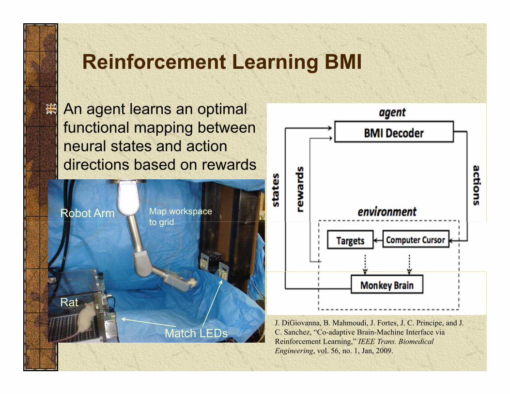
Reinforcement Learning BMIg
An agent learns an optimal f ti l i b tfunctional mapping between neural states and action directions based on rewards
Robot Arm Map workspace to gridto grid
J DiGi B M h di J F t J C P i i d J
RatJ. DiGiovanna, B. Mahmoudi, J. Fortes, J. C. Principe, and J. C. Sanchez, “Co-adaptive Brain-Machine Interface via Reinforcement Learning,” IEEE Trans. Biomedical Engineering, vol. 56, no. 1, Jan, 2009.
Match LEDs

Kernel Temporal Difference (λ)p ( )
Temporal Difference (λ) learningdIn multistep prediction of observation sequence
1( ) [ ( ) ( )]m
i t tt i
d y x y x y x+=
− = − 1( )my x d+
m 1 2, , , ,mx x x d
KLMS update rulet i=
( , ) ( ), ( )( ) ( )x x x x
y x y xκ φ φ
φ′ ′==
[ ( )] ( )i i iy y d y x xη φ← + −Kernel TD (0) update rule
( )11 , ( )) , ( ) ( )mi i iiy y y x y x xη φ φ φ+=← + −
( ) , ( )y x y xφ=
Kernel TD (λ) update rule
( )11 1, ( ) , ( ) ( )i km ii i ki ky y y x y x xη φ φ λ φ−+= =← + −

Q-learning via Kernel TD (λ)g ( )
Q-learningQ gBy setting the desired output as the cumulative reward
1 1 10k
i i k i i ikd r y r yγ γ∞+ + + +== = = +
TD error becomes
1 1 10i i k i i ik y yγ γ+ + + +=
[ ]1 1i i ir y yγ+ ++ −
Kernel TD (λ) update rule( )11 1, ( ) , ( ) ( )i km i
i i ki ky y y x y x xη φ φ λ φ−+= =← + − Q-learning via Kernel TD (λ) update rule
( )1 1, ( ) , ( ) ( )m i i k
i i i ky y r y x y x xη γ φ φ λ φ−+ +← + + − ( )1 11 1
, ( ) , ( ) ( )i i i ki k
y y y yη γ φ φ φ+ += =
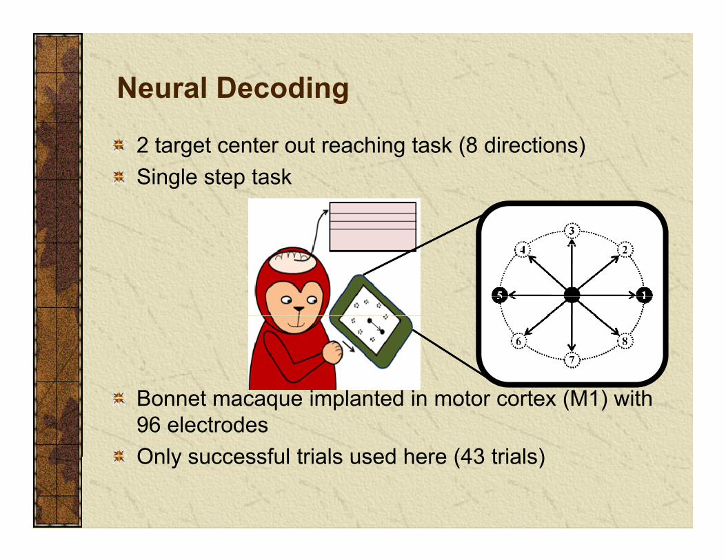
Neural Decodingg
2 target center out reaching task (8 directions)Single step taskSingle step task
Bonnet macaque implanted in motor cortex (M1) with 96 electrodesOnly successful trials used here (43 trials)Only successful trials used here (43 trials)

Kernel Temporal Difference (λ=0)( )
Neural States:100ms window185 units Q values Represent 8 from 96 channels6 taps
Q pdirections

ResultsFaster Convergence and Better Solution

Kernel Methods for Classification
In classification, the goal is to design the optimal separation surface between data classes Since KLMSseparation surface between data classes. Since KLMS is a universal mapper it can be used for classification replacing MLPs or even SVMsreplacing MLPs or even SVMs.
We proposed to use correntropy as a nonconvex approximation to the 0-1 loss ina nonconvex approximation to the 0 1 loss in classification
as followsas follows

Kernel Methods for Classification
We have shown that when kernel size σ=0.5 classifiers trained with KLMS perform as well as support vectortrained with KLMS perform as well as support vector machines.
They also do not overtrain! The issue is to find the global optimum since optimization is non convexglobal optimum since optimization is non convex.

Definition of Point Process
Point process is a stochastic process which describes a sequence of events occurring indescribes a sequence of events occurring in time
A spike train is a realization of a point processp p pspike train space
Q
• The probability measure over the spike train space defines a point process
P
}|)[iP { Δ Hdefines a point process
135
t}|),[inevent Pr{lim)|(
0 ΔΔ+=
→Δ
t
ttHtttHtλ

Neural Activityy
StimulationStimulationTime Resolution: 0.1ms Window Size: 100ms
Binned [0000000000001000000000010………00000000]Spike Train 1000 dimensions
Smoothed [000000000 1 0.73 0.54 0.39 0.21 0.1 0…000000]spike train 1000 dimensions
Spike time sequence(the most efficient) [0.023 0.045 0.076]
3 dimensions

Requirements for signal i ith ik t iprocessing with spike trains
O OMetric space k-Nearest Neighbor algorithm
O O O O OHilbert space
O O O OBanach space
O OMetric space k Nearest Neighbor algorithm
k-means algorithmSupport Vector Machine, Least squares, PCA CCAHilbert space
? ? ? ? ?Point processes?PCA, CCA, …
Most signal processing algorithms operate in Hilbert space
H t ik t i t Hilb t ?How to map spike trains to Hilbert spaces?
137

Functional Representation of Spike Trains Cross-intensity kernels
Given two point processes pi pj define theGiven two point processes pi, pj, define the inner product between their intensity functions
])|()|([
)|(),|(),()(2
=
=
T
jtp
itp
TL
jtp
itpji
dtHtHtE
HtHtppI
ji
ji
λλ
λλ
This yields a family of cross-intensity (CI) k l i t f th d l i d th
)|()|(T tptp ji
kernels, in terms of the model imposed on the point process history, Ht.
Paiva, et al Neural Computation, 2008

Functional Representation of Spike Trains
Spikernel (Shpigelman 2007) but it is created from binned data
Kernel Examples
binned data. Memoryless CI (mCI) kernel (Paiva 2008): For the Poisson process the inner product simplifies to
dtttI )()()( λλThis is the simplest of the CI kernels.Nonlinear cross intensity (nCI) kernel (Spike Kernel):
dtttppIji pT pji )()(),( λλ=
Nonlinear cross-intensity (nCI) kernel (Spike Kernel):dtttppI
ji pT pji ))(,)((),( λλκσσ =∗
with κσ a symmetric positive definite kernel, which is sensitive to nonlinear couplings in the time structure of the intensity functions.the intensity functions.

Functional Representation of Spike Trains
How to estimate mCI from dataHow to estimate mCI from data.
}1n:T][0{ii Nt =∈=s )()(ˆ
i
Ninttht
i
−=λ τs }1,...,n : T], [0{ ni iNt ∈s
λ
)U()exp()(
1
in
ini
n
n
tttttth −−−=−
=
ττ
is
)(i
tsλ
−=−−==i ji j N N
jn
im
N Nj
nT
imji ttdttthtthppI )()()(),(ˆ τκ
= == = m nnm
m nnT mji pp
1 11 1)()()()( τ

NCI Kernel
Inner product of two spike trains in Hilbert space
−−= 2
2ˆˆexp),(
σ
λλκσ
ji
jiss
ssFunction of two spike time sequences
H−+=−
jijjiiji
2,2,, λλλλλλλλ ssssssss
H
)s( iφ
)( jiji ss ,)(s),(s σκφφ == =
−−=
i jji
n m
mn ttN
1
N
12
NN
)exp(σ
is
js)s( jφ
Multi-Channel NCI Spike Kernel
2ˆˆ λλK
−−=∏
=2
1
exp),(σ
λλκσ
jk
ikK
kji
ssss

Somatosensory Stimulation
Thalamus Somatosensory cortex
DesignTactile Stimulation Neural response: spike trainsgMicro-stimulation
p p
[J. T. Francis 2008]

System Diagram
d1t
d2t
y1t
y2t
log likelihoody
λ1t
λ 2t
log likelihoodλ 2t
d1t
d2t
Inverse controller C(z) Plant model Ŝ(z) Plant S(z)
d2t
Li L., et al Proc. IEEE Neural Eng Conference, Cancun 2011

Adaptive Inverse Control
Take advantage of the novel kernel-based decoding methodology.
)(zP)(xφ cW)(xWy φ×= c
)(zφcW
1ˆ −pW
)()( zx φφ −= Δ
)()( 11 ˆˆ zWxW φφ ×−×= −− Δ pp
)( Δxφ

Biologically Plausible Neural Circuit (plant)
Model: 2 layer structurestructure
Layer 1 is input layer.
Layer 2 is 135 LIF neuron with sparse primarily local connectivity chosen to fit ydata from rat somatosensory cortex. (Maass 2002) Stimulation: 3D l t i fi ld3D electric field
Neuron response: Spike trains are recorded from 135 neurons

Time-invariant Plant)(ˆ zC )(zP
)( zC
)(ˆ zC
)(ˆ 1 zP−
)(zP
)(
120
Target firing pattern1
20
40
60
80
100
Cha
nnel
s
0.5
0.6
0.7
0.8
0.9
mila
rity
80
100
120
ls
System output
0
0.1
0.2
0.3
0.4Si
0 0.5 1 1.5 2
20
40
60
80
Time (s)
Cha
nne
0 20 40 60 80 100 1200
20
40
60
80
Channel
Firin
g R
ate
(Hz)

Redefinition of On-line Kernel Learning
Notice how problem constraints affected the form of theNotice how problem constraints affected the form of the learning algorithms.
On-line Learning: A process by which the freeOn line Learning: A process by which the free parameters and the topology of a ‘learning system’ are adapted through a process of stimulation by the p g p yenvironment in which the system is embedded.
Error-correction learning + memory-based learningg y gWhat an interesting (biological plausible?) combination.

Impacts on Machine Learning
KAPA algorithms can be very useful in large scale g y glearning problems.
Just sample randomly the data from the data base and p yapply on-line learning algorithms
There is an extra optimization error associated with pthese methods, but they can be easily fit to the machine contraints (memory, FLOPS) or the processing time constraints (best solution in x seconds).
Information Theoretic Learning (ITL)Information Theoretic Learning (ITL)
This class of algorithms canThis class of algorithms can be extended to ITL costfunctions and also beyond Regression (classification,Clustering, ICA, etc). See
IEEESP MAGAZINE, Nov 2006
Or ITL resource l fl dwww.cnel.ufl.edu


