Online Knowledge Enhancements for Monte Carlo Tree Search in Probabilistic Planning Bachelor Thesis Natural Science Faculty of the University of Basel Department of Mathematics and Computer Science Artificial Intelligence http://ai.cs.unibas.ch Examiner: Prof. Dr. Malte Helmert Supervisor: Dr. Thomas Keller and Cedric Geissmann Marcel Neidinger [email protected]2014-050-280 09/02/2017
Transcript
Online Knowledge Enhancements forMonte Carlo Tree Search in Probabilistic
PlanningBachelor Thesis
Natural Science Faculty of the University of Basel
Department of Mathematics and Computer Science
Artificial Intelligence
http://ai.cs.unibas.ch
Examiner: Prof. Dr. Malte Helmert
Supervisor: Dr. Thomas Keller and Cedric Geissmann
Playing board games is an activity traditionally associated with humans and for a long time,
humans deemed themselves unbeatable in this abstract type of problem where a player has
to ”think outside the box”, and show ”real intelligence” to beat their opponent. However
when IBM’s Deep Blue defeated chess champion Garri Kasparow in 1997 this dominant role
came to an end. Almost 20 years later, in 2016, Google’s AlphaGo software won a best of
five game of Go against South Korean Go master Lee Sedol under tournament settings. Go
is a highly complex strategy game that was, due to its complexity, considered to be one of
the last frontiers in AI game playing.
For a computer to be able to beat a human player it needs a plan, a sequence of actions
that lead to a desired goal state. While there are deterministic planning problems, the game
of Go is based around probabilities, for example about an opponent’s move. This leads
to probabilistic planning problems that can be described by a Markov Decision Process.
MDPs provide a framework for describing problems with a partially random outcome. In
the domain of Go this means that, while the computer has full control over its own moves,
the opponent’s moves are subject to a probability distribution.
While MDPs can be used to formalize probabilistic planning tasks we need an algorithm to
solve them. For AlphaGo Google used the class of Monte Carlo Tree Search algorithms to
solve the Markov Decision process. MCTS algorithms are a technique that has an increasing
popularity among researchers, especially in the domain of computer Go.
The goal of a planning algorithm is to find a series of actions that, once applied from a given
start state, lead to a goal state. To find such a plan we need to build a search tree. In many
cases this search tree can branch out very fast. MCTS overcomes this problem by building
a partial search tree. To build this tree a MCTS algorithm consists of four phases and has
two main components. In the first phase, a selection, the known region of the search tree is
traversed and the next, most urgent node is selected by a tree policy. Here, nodes that have
been visited more often in previous runs are selected more likely while still choosing actions
that have not been selected too often. In the following expansion phase the encountered
Introduction 2
leaf node is expanded. Leaving the known regions of the tree in the simulation phase a
default policy is used to simulate the run further down until either a final state is reached
or the algorithm runs out of computational budget. The last part is the backpropagation
phase in which all statistics of the tree are updated according to the results from the current
simulation.
With the MCTS algorithm being a framework there is no definitive way to implement the
different components. One widely used implementation of MCTS methods is the Upper
Confidence Bound applied to Trees(UCT)[?]. For action selection within the tree policy, it
uses the Bandit-based model of Upper Confidence Bounds(UCB) that was first introduced
in 2002[?]. Within UCB, in every state, the selection of the next action is modelled as a
k-armed bandit from which one arm has to be chosen. UCT applies this concept to trees,
inheriting UCBs desirable property of balancing exploration and exploitation.
With the wide application of MCTS in game playing agents, especially in the field of com-
puter Go, research has focused on finding improvements that yield better results in the field
of AI game playing, modifying standard algorithms to find the best game move faster.
In this thesis, first the MCTS framework as well as the UCB and UCT algorithms for action
selection are introduced in Chapter 2.
Chapters 3 and 4 then summarize different ways to increase the execution speed of Monte
Carlo Tree Search methods. Chapter 3 focuses on the field of All Moves as First(or shorter
AMAF) enhancements, that have proven to be effective in computer go. These modifications
are applied to a probabilistic planning scenario and are implemented in the probabilistic
planning framework PROST[?].
The family of All Moves as First enhancements is based on the idea of treating each action
as if it was the first action selected. This technique was first proposed in 1993[?] and has
been very successfully applied to game playing in the MCTS context. In this thesis, α-
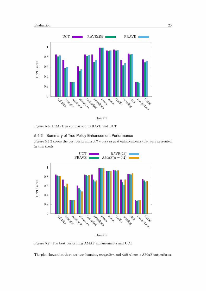
AMAF, Cutoff-AMAF and Rapid Action Value Estimation (RAVE) are implemented and
evaluated.
All of the performance enhancements discussed before have in common that they are part
of the node selection process. Therfore they only modify the tree policy. In Chapter 4
modifications to the backpropagation and simulation steps are introduced. In order to op-
timize results, modifing the default policy generally requires domain specific knowledge. To
maintain the domain independence of PROST, sampling techniques in backpropagation en-
hancements that don’t need domain specific knowledge are implemented and benchmarked.
The Move-Average Sampling Technique(or shorter MAST), an action’s value is stored in-
dependent of the state it is selected in. The rationale behind this is that actions that have
a higher average value might be a good choice. While MAST favors actions that are good
on average, Predicate-Average Sampling Technique (or shorter PAST) uses the predicates
valid in each state to favor actions that performed well in certain settings. MAST is then
implemented in PROST and benchmarked against other default policies.
Chapter 5 presents a performance evaluation of the methods introduced in the chapters
before.
2Background
In order to find a solution to a given planning task one has to find a correct set of ac-
tions which, after beeing applied to an initial state, yield the desired return. One way to
model such a process is using a Markov Decision process(or shorter MDP) which describes
a decision making process in a setting where the outcome is stochastic. More formally
Definition 1. A Markov Decision Process(MDP) is a stochastic model for decision
problems where the probability of selecting a new state only depends on the current state and
chosen action, not on historic decisions.
An MDP is a 5-tupel M = ⟨V, s0, A, T,R⟩ with
• A set of binary variables V inducing the set of states as S = 2V
• The initial state s0 ∈ S
• A set of applicable actions A
• A transition model T : S × A × S → [0; 1] that models the probability of reaching a
state s′ from s when action a was chosen.
• A reward function R(s, a)
A solution to an MDP is a policy.
Definition 2. A policy maps a state to an action
π : S → A (2.1)
One way of solving such a Markov decision process is the Monte Carlo Tree Search Frame-
work that has its roots in the application of Monte Carlo Methods and game theory to board
games. Here, the planning and execution are interleaved resulting in an iterative method so
that only the next step has to be simulated.
Monte Carlo methods emerged from applied physics and mathematics where they were used
to calculate integrals. The idea is to approximate the solution of a problem by randomly
sampling it a large number of times. Besides their initial use case these methods are used
for a large number of problems from risk management to weather forecasts.
Background 4
In a Monte Carlo Tree Search a decision tree made of nodes is built in memory. In the
context of this thesis a node in this tree can be defined as follows
Definition 3. A MCTS tree for a Markov Decision Problem M is made of nodes. In the i−th iteration of an MCTS algorithm a node V is a 5-tupel V = ⟨s,N (i)(s), N (i)(s, a), Q(i)(s, a), p(i)⟩with
• A state s ∈ S
• A counter N (i)(s) for the number of times the node has been visited in the first i
iterations
• A counter N (i)(s, a)∀a ∈ A for the number of times action a has been selected in state
s in the first i iterations
• A reward estimate Q(i)(s, a)∀a ∈ A for action a in state s after the i− th iteration
• A parent action p(i) that was selected in the (i− 1)− th node.
In order to solve the decision problem, in each node, the best action is searched. To do
so, an action’s reward must be estimated. The basic idea of MCTS is that the number of
times an action has been sampled in Monte Carlo approach can be used to approximate this
move’s[?] reward or value.
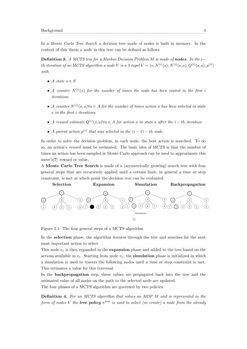
A Monte Carlo Tree Search is made of a (asymetrically growing) search tree with four
general steps that are recursively applied until a certain limit, in general a time or step
constraint, is met at which point the decision tree can be evaluated.
Selection
1
2
1
3
3 2 5
4
4
Expansion
1
2
1 2
3
3 2 5
4
4
Simulation
1
2
1 2
e
Simulation
3
3 2 5
4
4
Backpropagation
1
2
1 2
3
3 2 5
4
4
Figure 2.1: The four general steps of a MCTS algorithm
In the selection phase, the algorithm iterates through the tree and searches for the next
most important action to select.
This node ve is then expanded in the expansion phase and added to the tree based on the
actions available in ve. Starting from node ve, the simulation phase is initialized in which
a simulation is used to travers the following nodes until a time or step constraint is met.
This estimates a value for this traversal.
In the backpropagation step, these values are propagated back into the tree and the
estimated value of all nodes on the path to the selected node are updated.
The four phases of a MCTS algorithm are governed by two policies.
Definition 4. For an MCTS algorithm that solves an MDP M and is represented in the
form of nodes V the tree policy πtree is used to select (or create) a node from the already
Background 5
known part of the search tree. It governs the selection and expansion phase [?]. The tree
policy is stationary and maps the state of a node v to an action a.
πtree : V → a (2.2)
It estimates a reward value Q(i)πtree(s, a) for a state s and action a under policy πtree.
Definition 5. A default policy πdefault is used to simulate a process upon reaching an un-
known part in the tree in order to estimate a value for this path[?]. It governs the simulation
phase and is non-stationary.
Algorithm 1 shows the general MCTS algorithm[?].
Algorithm 1 General MCTS algorithm
function MctsSearch(s0)create root node v0 with state s0while within computational budget do
vl ← TreePolicy(v0)∆← DefaultPolicy(s(vl))
Backup(vl,∆)end whilereturn a(BestChild(v0))
end function
Originally used to approximate integrals in statistical physics, Abramson[?] suggested a
method of approximating an action’s estimated reward, its Q-value using this method.
Definition 6. The Q-value describes an action’s reward based on the state it is executed
on. An optimal policy always maps the action with the highest Q-value. Another policy π
estimates this reward value in a node v with state s. It’s value in the i− th iteration of the
algorithm can be approximated using
Q(i)π (s, a) =
1
N (i)(s, a)
N(i)(s)∑i=1
I(i)(s, a)z(i)(s) (2.3)
where z(i)(s) is the result of the i-th simulation played out from s and I(i)(s, a) is defined as
I(i)(s, a) =
1, if πtree(v) = a
0, otherwise(2.4)
Choosing an action randomly as a default policy this lazy Monte Carlo Tree search can
already be applied to real life examples such as Bridge or Scrabble, however there are
examples where influencing the action that will be selected based on past experience is
helpful. This leads to more advanced selection techniques such as UCT that will be described
in the following sections.
If it is known that the tree policy converges against the optimal policy, an additional benefit
of this method is that MCTS algorithms are ”statistical anytime algorithms for which more
computing power generally leads to better performance”[?]. This means that results can be
increased by simply allowing for more computing time.
Background 6
In itself, Monte Carlo Tree Search is just a framework for many different kinds of selection
algorithms that base around two concepts. First, an actions value might be approximated
using random simulation, and second these Q-values might be used to guide a policy towards
a good strategy. This means that a policy learns from previous results and improves over
time. Therefore MCTS does not build full game trees such as a simple BFS approach but
rather a partial tree whoms exploration is guided using previous results as an estimate of
an action’s value. The estimates of these ”best moves” become more accurate as the tree
grows.
In the following sections some basic algorithms shall be defined and explained.
2.1 Upper Confidence Bound for Trees(UCT)One possible algorithm for Monte Carlo Tree Search algorithms is the UCT algorithm[?]
first proposed in 2006.
The major problem for a tree policy is to balance the exploitation of already known good
actions with the exploration of actions that might not be the best choice in this node but
may yield a higher reward in the future.
To tackle this exploitation-exploration dilemma UCT introduces the concept of Upper Con-
fidence Bound(UCB) methods into the MCTS algorithm.
2.1.1 Bandit-Based Methods and Upper Confidence Bounds(UCB)In a bandit problem, one has to choose from K actions in every subsequent state. This
scenario is comparable to choosing an arm among the K arms of a multi-armed bandit,
hence the name. The goal is to maximise the cumulative reward from the chosen arm over
all states. In theory, this is done by always choosing the action that yields the biggest
reward. In practice however, the reward’s distribution for each action is unknown.
An estimate which arm Xj,n among the Xi,n1 ≤ i ≤ K,n ≥ 1 possible arms should be
chosen might be drawn from past experience upon an arm’s reward. However, there might
be other arms that offer an even higher reward to the player than the one currently believed
to be the best. This is also known as the exploitation-exploration dilemma[?] where one has
to balance between exploiting the currently believed to be optimal action with exploring
other actions that might turn out to be more rewarding in subsequent playouts.
In UCB an arms reward is estimated by
UCB1(aj) = Xj︸︷︷︸exploitation
+
√2 lnn
nj︸ ︷︷ ︸exploration
(2.5)
and the policy chooses the arm Xj , and therfor action aj , where
UCB1 = max {UCB1(aj)} ∀j (2.6)
Here, Xj is the average reward from arm j, nj is the number of times arm j was played and
n is the overall number of playouts.
Background 7
As indicated in the equation, the two parts balance exploration and exploitation. Choosing
the action that has the maximal average return emphasises the past knowledge while the
exploration term emphasises arms that haven’t been selected previously.
2.1.2 UCT algorithmThe UCB implementation has the desirable effect of balancing exploitation and exploration.
Especially its property of being in range of the best possible bound on the growth of regret
makes UCB a fitting algorithm for MCTS problems[?]. Upper Confidence Bounds(UCT)
takes this approach into search trees by treating the act of choosing a child node as a multi-
armed bandit problem where A is the set of K actions available. The expected reward Xj
from the UCB calculation is taken from the reward approximated by Monte-Carlo simula-
tions and thus is a random variable with unknown distribution as stated in a multi-armed
bandit problem.
In the i− th iteration of the algorithm, estimate the UCT score of a child node vj with the
parent node vl as
UCT (vl, vj) = Q(i)(sl, aj) + 2Cp
√2 lnN (i)(sl)
N (i+1)(sj)(2.7)
Where aj is the action leading from node vl to node vj and Cp > 0 a constant factor. This
factor can be used to control the impact of the exploration on node selection. A standard
value of Cp = 1√2can be found in literature.
From parent node vl select the child node v∗ that maximizes
v∗ = maxvj{UCT (nl, nj)} (2.8)
Since UCT is the most-used selection method in the context of MCTS, it will be used as
the baseline for evaluation of enhancements.
2.2 Default PolicyIn order to estimate the outcome of a run beyond the known state of the tree a default
policy is used to simulate the run upon expansion.
2.2.1 Random WalkThe basic UCT implementation proposed a random walk. Here a random action is selected.
While this method is easy to implement it does not guide the default policy towards more
promising actions.
2.2.2 IDSA more sophisticated approach is Iterative Deepening Search(or shorter IDS). Here, a limited
depth first search is conducted and the search depth is incremented in every step.
3All Moves as First (AMAF) Enhancements
The idea of All Moves as First heuristics have their roots in MCTS algorithms for computer
Go. They originated from history heuristics that try to leverage history information to
enhance action selection on the Tree-level as well as on the tree-playout level that tries to
improve the simulation using historic information. The general idea of history heuristics is
to approximate an initial action value from history.
For All Moves as First enhancements, the statistics of all actions selected during the simula-
tion process are treated as if they were the first action applied. This means that all actions
selected during selection and simulation are treated equally as if they were previously played
out.
A reward estimate generated from the AMAF heuristic is generally referred to as the AMAF
score A.
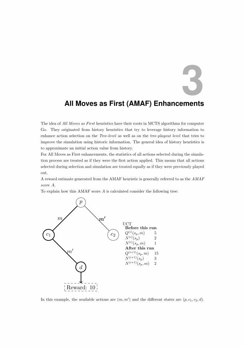
To explain how this AMAF score A is calculated consider the following tree:
m m′m′
m′
Reward: 10
p
c1 c2
d
UCTBefore this runQ(i)(sp,m) 5N (i)(sp) 2N (i)(sp,m) 1After this runQ(i+1)(sp,m) 15N (i+1)(sp) 3N (i+1)(sp,m) 2
In this example, the available actions are (m,m′) and the different states are (p, c1, c2, d).
All Moves as First (AMAF) Enhancements 9
After some trials the tree policy chooses the bold printed playout path p → c1 → d by
selecting actions m,m′. For normal UCT backup in Node p with state sp, the update
would increment the number of visits by 1 and add the reward from this trial as shown
in the table to the right. AMAF keeps an additional table and would additionally update
the Q(i+1)AMAF (sp,m
′) pair with the reward from this trial, even tough it was not the action
directly selected in p but it was selected in a subsequent move. Also the NAMAF (sp,m′)
counter that counts the number of times the AMAF score for action m′ in state sp has been
updated is incremented.
All Moves as First enhancements have proven to be very efficient in the context of computer
Go. The following sections outline some AMAF enhancements that will be benchmarked
against pure UCT.
3.1 α-AMAFWhen selecting actions, one could solely rely on the AMAF score for selecting the next
action. However the UCT score still carries value so α-AMAF seeks to combine the two
approaches.
The total score for an action is a linear combination of AMAF score and UCT score with
SCT = αA+ (1− α)U (3.1)
Here, U is the UCT score and A the AMAF-score. α is a weighting factor that determines
which part should influence the score more.
In the example above, the UCT score for action m′ in the node p with state sp would be:
U = Q(i)(sp,m) + 2Cp
√ln(N (i)(sp))
N (i+1)(sc1)(3.2)
In α-AMAF this value would then be biased with
A =1
NAMAF (sp,m′)QAMAF (sp,m
′) (3.3)
using the linear weight function introduced above.
3.2 Cutoff-AMAFCutoff-AMAF is closely related to α-AMAF. The idea is to initialize the tree with some
AMAF data but rely on the more accurate UCT data later in the search process. Therefore,
the score α-AMAF score is used for the first k simulations after which only the UCT score
is used. This gives
SCT =
αA+ (1− α)U , for i ≤ k
U else(3.4)
where i is the current episode obtained from the search node.
All Moves as First (AMAF) Enhancements 10
3.3 Rapid Action Value Estimation(RAVE)Rapid Action Value Estimation, or shorter RAVE, was first introduced in a 2007 paper [?].
The aim of RAVE is to exploit the already exisiting structure of the search tree to get a
rapid evaluation of an actio’s cost and reward.
A general bottleneck in UCT based MCTS algorithms is, that an action a from a state s
has to be sampled multiple times in order to get reliable values. With large action spaces
this can lead to a slow down.
As opposed to UCT, where an action is valued based on the number of times it was selected,
RAVE averages the return of all episodes where a was selected at any subsequent time[?].
RAVE seeks to combine this approach with the idea of α-AMAF. While the parameter α
in α−AMAF is static, RAVE uses a calculated value for α that depends on the number of
times a node is visited. This is a softer approach to cutoff AMAF. Instead of only using the
UCT score after a certain amount of trials, RAVE favors the UCT score for nodes that have
been visited multiple times while using the quicker updated but more variant AMAF score
A for less visited nodes.
First introduce a new paramter V > 0. Then calculate the value of α according to
α = max
{0,
V − v(n)
V
}(3.5)
The parameter V yields the number of visits to a node befor the RAVE values are not
considered anymore.
4Backpropagation Enhancements
In standard MCTS, the default policy randomly selects an action a among all available
options. The advantage of using such an approach is the domain independence of the
technique. There is no domain knowledge required and the randomness ensures that all
states are covered, given enough trials. However, this is not realistic as a human player in,
for example, a board game would not randomly select an action but rather use knowledge
to determine a promising action. Incorporating offline knowledge, action selections based
on databases or expert games, is beyond the scope of this thesis, but rather this will focus
on using online knowledge gained from self-play and learning.
4.1 Move-Average Sampling Technique (MAST)Move-Average Sampling Technique (or shorter MAST) has a similar approach to history
heuristics. The idea is, that moves or actions that were good previously might be good in
another state. MAST uses this idea and keeps a table in which the average reward Q(a)
independent of state is stored.
In subsequent moves, the default policy uses a Gibbs distribution to bias selection using
these MAST values. It selects an action according to the probability
P (a) =e
Q(a)τ
n∑b∈A
eQ(b)
τ
(4.1)
Here, P (a) is the probability of action a being selected and A is the set of actions available.
Q(a) is an action’s average return value over previous playouts and τ is a stretching param-
eter of the distribution and controls how much influence the Q(a) value should have on the
action selection. τ → 0 stretches the distribution while higher values of τ make it converge
towards a uniform action selection. This selection enhancement was first introduced for
CadiaPlayer[?] and biases the selection towards moves that were good on average.
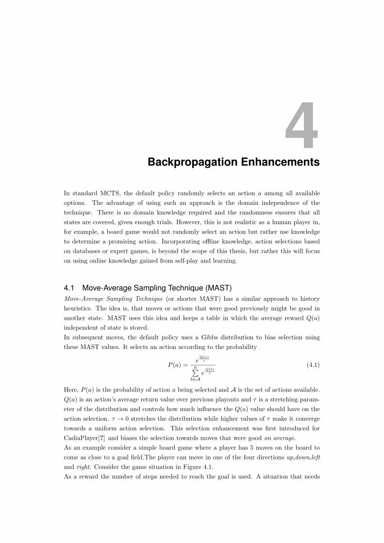
As an example consider a simple board game where a player has 5 moves on the board to
come as close to a goal field.The player can move in one of the four directions up,down,left
and right. Consider the game situation in Figure 4.1.
As a reward the number of steps needed to reach the goal is used. A situation that needs
Backpropagation Enhancements 12
Player
Goal field
Movepath
Figure 4.1: Sample game situation for the example board game
one more move to get to the finish would have a reward of 5 − 1 = 4 and would therefor
be considered a good move. It’s easily visible that either moving up four times and then
moving right or moving right and then moving up four times is the best way.
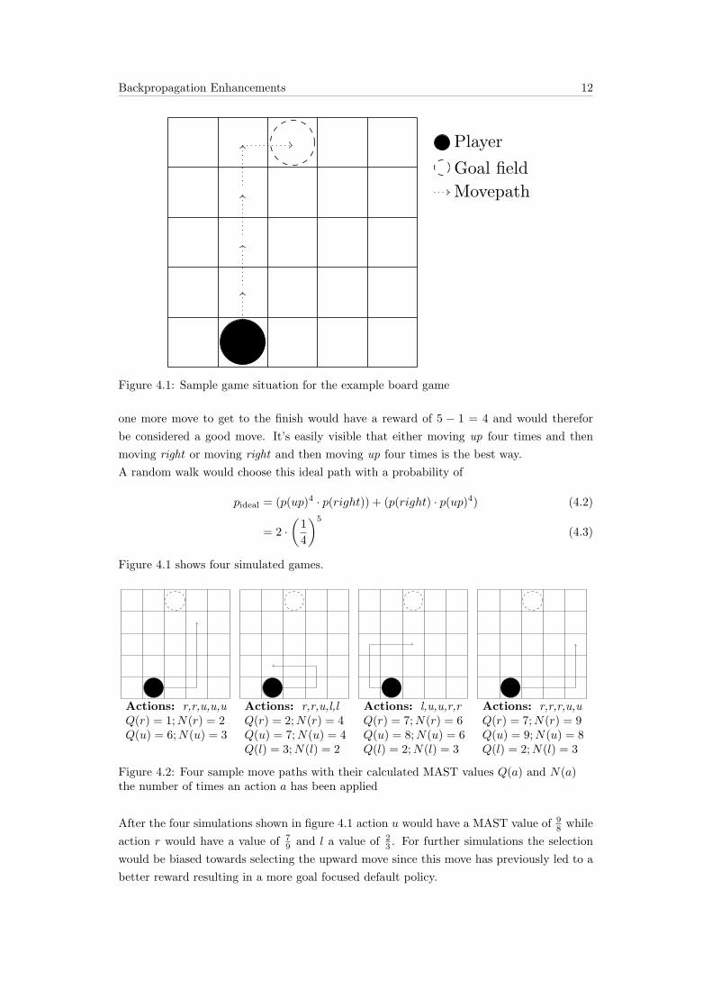
A random walk would choose this ideal path with a probability of