Page 1
Online model calibration for a simplified LES model in pursuit ofreal-time closed-loop wind farm controlBart Doekemeijer1, Sjoerd Boersma1, Lucy Pao2, Torben Knudsen3, and Jan-Willem van Wingerden1
1Delft Center for Systems and Control, Delft University of Technology, The Netherlands2Electrical, Computer & Energy Engineering, University of Colorado Boulder, Colorado, United States of America3Department of Electronic Systems, Aalborg University, Denmark
Correspondence: B.M. Doekemeijer ([email protected] )
Abstract. Wind farm control often relies on computationally inexpensive surrogate models to predict the dynamics inside a
farm. However, the reliability of these models over the spectrum of wind farm operation remains questionable due to the many
uncertainties in the atmospheric conditions and tough-to-model flow dynamics at a range of spatial and temporal scales relevant
for control. A closed-loop control framework is proposed in which a simplified dynamical LES model is calibrated and used
for optimization in real time. This paper presents an estimation solution with an Ensemble Kalman filter (EnKF) at its core,5
which calibrates the surrogate model to the actual atmospheric conditions. The estimator is tested in high-fidelity simulations
of a nine-turbine wind farm. Using exclusively turbine SCADA measurements, the adaptability to modeling errors and changes
in atmospheric conditions (TI, wind speed) is shown. Convergence is reached within 400 seconds of operation, after which
the estimation error in flow fields is negligible. At a low computational cost of 1.2 s on an 8-core CPU, this algorithm shows
comparable accuracy to the state of the art from the literature while being approximately two orders of magnitude faster. Using10
the calibration solution presented, the surrogate model can be used for accurate forecasting and optimization.
1 Introduction
Over the past decades, global awakening on climate change and the environmental, political and financial issues concerning
fossil fuels have been catalysts for the growth of the renewable energy industry. As the primary energy demand in Europe
is projected to decrease by 200 million tonnes of oil equivalent from 2016 to 2040, there is an additional shift in the energy15
source used to meet this demand (International Energy Agency, 2017). Shortly after 2030, onshore and offshore wind energy
are projected to become the main source of electricity for the European Union. By then, about 80% of all new capacity added
is projected to come from renewable energy sources, enabled by a favorable political climate.
While there are clear benefits in the growth of the wind energy industry, an important problem with wind energy is that
almost all commercial turbines are currently disconnected from the electricity grid by their power electronics (Aho et al.,20
2012). As the current grid-connected fossil fuel plants are replaced by grid-disconnected renewable energy plants, the inertia
of the electricity grid will decrease. Thus, the grid will become less stable, making it more prone to machine damage and
blackouts (Ela et al., 2014). Therefore, there is a strong need for wind farms and other renewables to provide ancillary grid
services. Wind farm control aimed at increasing the grid stability is more commonly defined as active power control (APC). In
1
Wind Energ. Sci. Discuss., https://doi.org/10.5194/wes-2018-33Manuscript under review for journal Wind Energ. Sci.Discussion started: 26 April 2018c© Author(s) 2018. CC BY 4.0 License.
Page 2
APC, the power production of a wind farm is regulated to meet the power demand of the electricity grid, which may change
from second to second.
Existing literature on wind farm control has focused mainly on maximizing the power capture (e.g., Rotea, 2014; Gebraad
and van Wingerden, 2015; Gebraad et al., 2016; Annoni et al., 2016a; Munters and Meyers, 2017; Vali et al., 2017). Though,
literature on APC has been receiving an increasing amount of attention (e.g., Fleming et al., 2016; Van Wingerden et al.,5
2017; Boersma et al., 2017a). The main challenges in wind farm control are the large time delays caused by the formation of
wakes, the many uncertainties in the atmospheric conditions, and the questionable reliability of surrogate models over the wide
spectrum of wind farm operation (see Boersma et al. (2017a) and Knudsen et al. (2015) for state-of-the-art overviews of control
and control-oriented modeling for wind farms). While there has been success with model-free methods for power maximization
(e.g., Rotea, 2014), it is unclear to what degree such methods can be used for power forecasting. Furthermore, model-free10
methods typically have long settling times, making these methods intractable for APC. On the other hand, for model-based
approaches, the aforementioned challenges make it impossible for any model to reliably provide power predictions in an open-
loop setting. Hence, a model-based approach in which a surrogate wind farm model is actively adjusted to the present conditions
is a necessity for reliable and computationally tractable APC algorithms. This closed-loop wind farm control framework is
displayed in Fig. 1. The control framework of Fig. 1 requires three components.15
External conditions
plant
+
Measurement noise
+q z
Modeladaptation
−z+
(z − z )
Model-basedoptimization
xControl objective
controller
March 29, 2018 1 / 1
Figure 1. Closed-loop wind farm control framework. Measurements z (e.g., SCADA, met mast, LiDAR data) are fed into the controller
block. First, the state of the surrogate wind farm model x is estimated to represent the actual atmospheric and turbine conditions inside
the wind farm. Secondly, using the calibrated model, an optimization algorithm determines the control policy (e.g., yaw angles, blade pitch
angles) for all turbines q . This control policy may be a set of constant operating points, but can also be time-varying, depending on whether
the surrogate model is time-varying and the employed optimization algorithm.
The first component of the closed-loop framework is a computationally inexpensive control-oriented surrogate model that
accurately predicts the power production of the wind farm ahead in time, on a time-scale relevant for control. The most
2
Wind Energ. Sci. Discuss., https://doi.org/10.5194/wes-2018-33Manuscript under review for journal Wind Energ. Sci.Discussion started: 26 April 2018c© Author(s) 2018. CC BY 4.0 License.
Page 3
commonly used surrogate models in wind farm control are steady-state models, which are heuristic and neglect all temporal
dynamics (Boersma et al., 2017a). Thus, wind farm control algorithms synthesized using such models neglect any transient
dynamics in the wind farm, thereby potentially limiting performance. While some of these models have shown success in wind
tunnel tests (e.g., Schreiber et al., 2017) and field tests (e.g., Fleming et al., 2017a, b) for power maximization, the actuation
frequency is limited to the minutes-scale, since the flow and turbine dynamics are predicted on the minute-scale. Furthermore,5
time-ahead predictions with these models are limited to the time-invariant steady-state, limiting their use for APC.1 There is a
smaller yet significant number of dynamic surrogate wind farm models (e.g., Munters and Meyers, 2017; Boersma et al., 2017b;
Shapiro et al., 2017a), which attempt to model the dominant temporal dynamics inside the farm. These models can be used for
control on the seconds-scale, and furthermore allow time-ahead predictions, some even under changing atmospheric conditions.
Specifically, the dynamic surrogate model employed in Shapiro et al. (2017a) is computationally feasible, but only models the10
flow in one dimension, and furthermore allows no turbine yaw or changes in the wind direction, limiting its applicability.
Furthermore, the dynamical model in Munters and Meyers (2017) has shown success for closed-loop control applications, but
as it is a 3D LES code, it is much too computationally costly for any kind of real-time control, and the authors present their
results solely as a benchmark case. In the work presented here, the model described in Boersma et al. (2017b) is used, which is
a light-weight two-dimensional LES code with wind farm control as its main objective. This dynamic surrogate model, named15
“WindFarmSimulator” (WFSim), includes yaw and axial induction actuation, turbine-induced turbulence effects, and spatially
and temporally varying inflow profiles, with a moderate computational cost (101− 102 ms per timestep).2
The second component of the closed-loop framework is an algorithm that adjusts the surrogate model’s parameters to im-
prove its accuracy online using flow and/or turbine measurements (e.g., SCADA data, LiDAR measurements, met masts). In
terms of control, this turns into a dual estimation problem, in which both the model state and a subset of model parameters20
are estimated online. Currently, the optimization algorithms presented in Munters and Meyers (2017) and Vali et al. (2017)
have assumed full state knowledge, conveniently ignoring the step of model adaptation. Literature on state reconstruction and
model calibration for dynamical wind farm models is sparse, limited to linear low-order models and/or common estimation
algorithms. Gebraad et al. (2015) designed a traditional Kalman filter (KF) for their low-fidelity “FLORIDyn” model, sho-
wing marginal improvements compared to optimization using a static model. Shapiro et al. (2017a) present a one-dimensional25
dynamic wake model used with receding horizon control for secondary frequency regulation, using an estimation algorithm
following Doekemeijer et al. (2016). Furthermore, Iungo et al. (2015) used dynamic mode decomposition to obtain a reduced-
order model of the wind farm dynamics, which was then combined with a traditional KF for state estimation. To the best of
the authors’ knowledge, none of these methods have explored more sophisticated models such as WFSim, and often only use
simple state estimation algorithms that are lacking in terms of accuracy and in terms of computational tractability.30
The third component of the closed-loop framework is an optimization algorithm, which typically is a gradient-based or
nonlinear optimization algorithm (e.g., Gebraad et al., 2016; Thomas et al., 2017) for steady-state models, and a model-based
1Control using steady-state models is typically limited to an actuation frequency of every 5-10 minutes, depending on the wind speed and size of the
farm. Namely, after each change in control settings, it takes minutes before the flow propagates through the farm and a steady-state is formed. In steady-state,
SCADA data is then temporally averaged, upon which a new set of control parameters is calculated for the current atmospheric conditions.2For a more detailed analysis on the computational cost involved in WFSim, the reader is referred to Boersma et al. (2017b).
3
Wind Energ. Sci. Discuss., https://doi.org/10.5194/wes-2018-33Manuscript under review for journal Wind Energ. Sci.Discussion started: 26 April 2018c© Author(s) 2018. CC BY 4.0 License.
Page 4
predictive optimization method for dynamical models (e.g., Goit and Meyers, 2015; Vali et al., 2017; Siniscalchi-Minna et al.,
2018). A more in-depth discussion on optimization algorithms for the framework of Fig. 1 is out of the scope of this article,
and therefore not further continued here.
The focus of this work is on a model adaptation algorithm for WFSim, which trades off estimation accuracy with computa-
tional complexity for online model calibration. In previous work (Doekemeijer et al., 2016, 2017), recursive state estimation5
using flow measurements downstream of each turbine has shown success using an Ensemble KF (EnKF), with a computational
cost several orders of magnitude lower than traditional KF methods. The main contributions of this article are 1) the addition
of adaptation to time-varying atmospheric conditions (specifically, the freestream wind speed and turbulence intensity), which
is of crucial importance for accurate longer-term forecasting, 2) each turbine’s power signal can now be used in addition to, or
instead of, flow measurements, as power measurements are readily available in existing farms, in contrast to flow measurements10
(other than the hub anemometer, which yields low-quality measurements), 3) the computational complexity is further reduced
compared to previous work, and 4) the EnKF algorithm will be compared to the state of the art algorithms in the literature.
The structure of this article is as follows. In Section 2, the surrogate model will be described in more detail. In Section 3,
a time-efficient, online model calibration algorithm for low- and medium-fidelity dynamical wind farm models is detailed.
This online calibration algorithm is tested against standard algorithms in the literature using high-fidelity simulation data in15
Section 4. The article is concluded in Section 5.
2 The surrogate model
To motivate the choice of model parameters that are to be estimated in real time, the surrogate model used in the work at hand
is outlined in this section. The chosen surrogate model is the WindFarmSimulator (WFSim) model presented by Boersma et al.
(2017b). In short, WFSim solves a modified set of unsteady two-dimensional (2D) Navier-Stokes equations in a horizontal20
plane at the turbine hub height. This surrogate model is a medium-fidelity nonlinear dynamic wind farm model with a total
of 5 tuning parameters. WFSim has shown success in reconstructing the flow field and turbine power signals of high-fidelity
LES data. This model is particularly suited for the framework presented in Fig. 1 as it is dynamic, includes both yaw and axial
induction control, handles temporally and spatially varying inflows, and yields a relatively high accuracy with a manageable
computational cost.25
In Section 2.1, the governing equations of the model are presented. The turbulence and turbine model are described in
Sections 2.2 and 2.3, respectively. The spatial and temporal discretization process is described in Section 2.4, including some
remarks about the boundary conditions and the computational tractability of the model.
2.1 Governing equations
The WFSim wind farm model is based on the two-dimensional unsteady incompressible Navier-Stokes (NS) equations to30
maintain computational tractability compared to a three-dimensional model. Furthermore, in WFSim the continuity equation
is modified to accommodate for flow dissipation in the neglected vertical dimension. The surrogate model can be described
4
Wind Energ. Sci. Discuss., https://doi.org/10.5194/wes-2018-33Manuscript under review for journal Wind Energ. Sci.Discussion started: 26 April 2018c© Author(s) 2018. CC BY 4.0 License.
Page 5
completely by the flow and rotor dynamics in a horizontal plane at hub height, derived from the following set of partial
differential equations:
∂u
∂t+ (u ·∇H)u + ∇H · τH + ∇H · p= f,
∂u
∂x+ 2
∂v
∂y= 0, where u =
[u v
]T, ∇H =
[∂∂x
∂∂y
]T, (1)
where u and v are the longitudinal and lateral flow velocity respectively, x and y are the spatial coordinates in longitudinal and
lateral direction respectively, τH is a 2D tensor containing the horizontal subgrid stresses (turbulence model), p is pressure,5
and f contains the forcing terms (turbine model) acting on the flow. Equation (1) deviates from the traditional 2D NS equations
in two ways. Firstly, the diffusion term is neglected, as it plays a negligible role in the dominant flow dynamics due to the low
viscosity of air. Secondly, the term ∂v∂y in the continuity equation is multiplied by a factor 2 to approximate flow dissipating in
the vertical flow dimension. See Boersma et al. (2017b) for a detailed derivation of (1).
2.2 Subgrid-scale (turbulence) model10
Boersma et al. (2017b) introduced a new model for the subgrid-scale term τH . The subgrid-scale model is formulated using
an eddy-viscosity assumption in combination with Prandtl’s mixing length model,
τH =−`u(x,y)2∣∣∣∂u
∂y
∣∣∣ ·(
12∇Hu + (∇Hu)T
), with `u(x,y) =
G(x′i,y
′i) ∗ `iu(x′i,y
′i), if x ∈ X and y ∈ Y,
0, otherwise,(2)
where `u(x,y) ∈ R+ is a local spatially varying parametrization of the mixing length, inspired by the high-fidelity simulation
results presented in Iungo et al. (2017). G(x′i,y′i) is a smoothing pillbox filter with radius 3, ∗ is the 2D spatial convolution15
operator, and X and Y define a rectangular region behind the turbine rotor to which the turbulence model applies, given by
X = {x : x′i ≤ x≤ x′i + cos(φ) · d}, Y = {y : y′i−D
2+ sin(φ) ·x′i ≤ y ≤ y′i +
D
2+ sin(φ) ·x′i},
with (x′i,y′i) the wind-aligned axis system centered at the turbine rotor,D the turbine rotor diameter, φ the mean wind direction
in the original (x,y)-axis system, and d a length parameter for the turbulence model. See Fig. 2 for a schematic drawing. Then,
`iu(x,y) is defined as20
`iu(x′i,y′i) =
(x′i− d′)`s, if d′ ≤ x′i ≤ d and −D2 ≤ y′i ≤ D
2 ,
0, otherwise,(3)
where `s defines the slope of `iu(x′i,y′i), and d′ is a second length parameter for the turbulence model. Thus, the entire turbulence
model has three tuning parameters: the length parameters d and d′ are the upper and lower spatial bounds, respectively, and `s
is a gradient parameter for the mixing length.
5
Wind Energ. Sci. Discuss., https://doi.org/10.5194/wes-2018-33Manuscript under review for journal Wind Energ. Sci.Discussion started: 26 April 2018c© Author(s) 2018. CC BY 4.0 License.
Page 6
ℓ ii
i
i
i
11
dℓi
d i
ℓ s=dℓ
i
d i
Figure 2. The subgrid-scale model implemented in WFSim employs a spatially varying mixing length parameter that increases with distance
behind the rotor. This can be explained by the turbine-induced turbulent structures in the wake. Image courtesy of Boersma et al. (2017b).
2.3 Turbine model
Turbine forces in WFSim are modeled using the classical non-rotating actuator disk model (ADM), projected onto the 2D
plane at hub height. The turbine forcing term in (1), f, at spatial location s =[x y
]T∈ R2 is expressed as
f =NT∑
i=1
fi, with fi =cf2C ′Ti
[Ui cos(γi)]2
cos(γi +φ)
sin(γi +φ)
·H
[D
2− ||s − t i||2
]· δ [(s − t i) · e⊥,i] , (4)
with H[•] the heaviside function, δ[•] the Dirac delta function, and e⊥,i ∈ R2 the unit vector perpendicular to the ith rotor disk5
with position t i ∈ R2. The scalar C ′Tiis a variation of the non-dimensional thrust coefficient of turbine i which can be related
to physical turbine parameters such as the generator torque and blade pitch angles (Goit and Meyers, 2015). The scalar γi is
the yaw angle of turbine i with respect to the incoming wind, and Ui is the average flow velocity over the rotor of turbine i.
The scalar cf is a static tuning variable to account for the time-invariant rotor dimensions and numerical grid effects, making
it the fourth tuning variable in WFSim. The control variables for optimization in the framework of Fig. 1 are γi and C ′Ti10
for i= 1, ...,NT , with NT the number of turbines. Furthermore, the instantaneous power capture of the wind farm Pfarm is
calculated in a similar approach by
Pfarm =NT∑
i=1
Pturb,i, with Pturb,i =cp2ρAC ′Ti
[Ui cos(γi)]3, (5)
with scalar cp the fifth tuning factor used to account for numerical grid effects and time-invariant turbine losses, andA the rotor
swept surface area. Note that C ′T has a direct mapping to the turbine power Pturb,i, and thus replaces the usual non-dimensional15
power coefficient, following the example of Goit and Meyers (2015).
6
Wind Energ. Sci. Discuss., https://doi.org/10.5194/wes-2018-33Manuscript under review for journal Wind Energ. Sci.Discussion started: 26 April 2018c© Author(s) 2018. CC BY 4.0 License.
Page 7
2.4 Discretization, boundary conditions, and computational cost
Equation (1) is spatially discretized on a quadrilateral grid employing the finite volume method and the hybrid differencing
scheme (Boersma et al., 2017b). Temporal discretization is performed using the implicit method, which guarantees stability of
the solution. Dirichlet boundary conditions for u and v are applied on one side of the grid for inflow, while Neumann boundary
conditions are applied on the remaining sides for the outflow. After discretization, the surrogate wind farm model described in5
this section reduces to a nonlinear discrete-time deterministic state-space model, described by
xk+1= f (xk,qk),
z k = h(xk,qk),
where xk ∈ RN is the system state at discrete time instant k ∈ Z, which is a column vector containing the collocated longi-
tudinal flow velocity at each cell in the domain uk ∈ RNu , the lateral flow velocity at each cell in the domain vk ∈ RNv , and10
the pressure term at each cell in the domain pk ∈ RNp , with N =Nu +Nv +Np and Nu ≈Nv ≈Np ≈ 13N . The state xk is
formulated as
xTk =
[uT
k vTk pT
k
].
Empirically, good results have been achieved with cell dimensions of about 30−50 m in width and length, resulting in N with
a typical value on the order of 103− 104 for medium-sized wind farms (e.g., Vali et al., 2016, 2017; Doekemeijer et al., 2016,15
2017; Boersma et al., 2017b). Such a number of states may seem very small for LES simulations, yet is very high for control
purposes. Furthermore, qk ∈ RO includes the system inputs, i.e., the turbine control settings γi and C ′Tifor i= 1, ...,NT . The
system outputs z k ∈ RM are defined by sensors. It can include, among others, flow field measurements (z k ⊂ xk) and power
measurements. We define the integer Mu,v ∈ Z with Mu,v ≤M as the total number of flow field measurements. The nonlinear
functions f and h are the state forward propagation and output equation, respectively.20
The computational cost may vary from 0.02 s for a small wind farm with N = 3 · 103 states (e.g., a 2 by 1 wind farm in
Doekemeijer et al. (2017)), to 1.2 s for N = 1 · 105 states for medium-sized wind farms (e.g., a 3 by 3 wind farm in Boersma
et al. (2017b)), for a single time-step forward simulation on a single desktop CPU core. This computational complexity is what
motivates the use of time-efficient estimation algorithms in the work at hand, and time-efficient predictive control methods for
optimization in related work (Vali et al., 2017). In this work, the limits of computational cost are explored to maximize model25
accuracy while still allowing real-time control.
3 Online model calibration
Due to the limited accuracy of surrogate wind farm models, and due to the many uncertainties in the environment, surrogate
models often yield predictions with significant uncertainty of the wind flow and power capture inside a wind farm. Since
control algorithms largely rely on such predictions, this may suppress gains or even lead to losses inside a wind farm. Unfortu-30
7
Wind Energ. Sci. Discuss., https://doi.org/10.5194/wes-2018-33Manuscript under review for journal Wind Energ. Sci.Discussion started: 26 April 2018c© Author(s) 2018. CC BY 4.0 License.
Page 8
nately, higher-fidelity models are computationally prohibitively expensive for control applications. Hence, rather, lower-fidelity
surrogate models are calibrated online using readily available measurement equipment.
In this section, first the challenges for real-time model calibration for the surrogate “WFSim” model described in Section 2
will be highlighted in Section 3.1. Secondly, a mathematical framework for recursive model state estimation will be presented
in Section 3.2. Thirdly, a number of state estimation algorithms are presented in Sections 3.3 to 3.6, building up from the5
industry standard to the state of the art in the literature. Finally, a robust, computationally efficient model calibration solution
is synthesized in Section 3.7, which allows the simultaneous estimation of the boundary conditions, model parameters, and the
model states of WFSim in real time using readily available measurements from the wind farm.
Note that we will henceforth refer to the estimation of x as state estimation. The estimation of tuning parameters, such as `s
and cf (Section 2), which are included in the expressions for f and h, are considered as parameter estimation.10
3.1 Challenges
Online model calibration for WFSim is challenging for a number of reasons. First of all, the model is nonlinear, and thus
the common linear estimation algorithms cannot be used without linearization. While analytical expressions for the linearized
surrogate model are available (Boersma et al., 2017b), the absence of linear expressions for the subgrid-scale model and the
multiple max-, min- and abs-operators in the nonlinear model limit its accuracy. Secondly, the surrogate model is sensitive to15
instability when the estimated state sufficiently deviates from the continuity equation in (1). In addition, while state estimation
(i.e., estimation of the instantaneous flow field) may prove helpful in short-term forecasting, calibration of additional model
parameters is necessary (e.g., the inflow/boundary conditions and the turbulence model) for reliable longer-term forecasting,
as will be shown in Section 4. Finally, the surrogate model typically has on the order of N ∼ 103− 104 states, which is
extraordinarily high for control applications. Though, real-time estimation is a necessity for real-time model-based closed-20
loop control, and thus one needs to find a trade-off between accuracy on the one hand, while guaranteeing updates at a low
computational cost on the seconds-scale on the other hand.
3.2 General formulation
This section details the basics of Kalman filtering, which is the literature standard for state estimation in control. The goal of a
Kalman filter (KF) is to estimate the unmeasured states of a dynamical system through noisy measurements. Assumed here is25
a system (the wind farm) represented mathematically by a discrete-time stochastic state-space model with additive noise,
xk+1= f (xk,qk)+wk, (6)
z k = h(xk,qk)+ vk, (7)
where k is the time index, x ∈ RN is the unobserved system state (in this case: the flow and pressure fields inside the wind
farm), z ∈ RM are the measured outputs of the system (e.g., flow measurements, SCADA data), f describes the forward-30
in-time state propagation mapping, h describes the output equation from state to measurement, q ∈ RO and w ∈ RN are
the controllable inputs and process noise respectively that drive the system dynamics, and v ∈ RM is measurement noise.
8
Wind Energ. Sci. Discuss., https://doi.org/10.5194/wes-2018-33Manuscript under review for journal Wind Energ. Sci.Discussion started: 26 April 2018c© Author(s) 2018. CC BY 4.0 License.
Page 9
Furthermore, we assume w and v to be zero-mean white Gaussian noise with covariance matrices
E
vk
wk
[vT
` wT`
]=
Rk ST
k
Sk Qk
∆k−`, where ∆k−` =
1, if k = `,
0, otherwise,(8)
with E the expectation operator. Estimates of the state xk, denoted by xk|k, are computed based on measurements from the
real system. Here, xk|` means an estimate of the model’s state vector x at time k, using all past measurements and inputs Z`,
as5
xk|` = E[xk|Z`] , with Z` = z 0,z 1,z 2 . . .z `, q0,q1,q2 . . .q `. (9)
State estimates are based on the internal model dynamics and the measurements, weighted according to their respective proba-
bility distributions. We aim to find an optimal state estimate, in which optimality is defined as unbiasedness, E[xk − xk] = 0,
and when the variance of any linear combination of state estimation errors (e.g., the trace of E[(xk − xk)(xk − xk)T
]) is
minimized (Verhaegen and Verdult, 2007).10
In reality, the assumed model described by f and h always has mismatches with the true system, and the assumptions in (8)
often do not hold. Further, the matrices Qk, Rk, and Sk are usually not known and rather considered tuning parameters. In
practice, the values of R and Q are used to shift the confidence levels between the internal model and the measured values.
For R�Q , estimations will heavily rely on the measurements, while for Q �R, estimations will mostly rely on the internal
model. Kalman filtering remains one of the most common methods of recursive state estimation, as it has proven successful in15
many applications. KF algorithms typically consist of two steps, namely:
1. A state and output forecast, including their uncertainties (covariances):
xk|k−1 = E[f (xk−1,qk−1) +wk−1|Zk−1
], (10)
z k|k−1 = E[h(xk,qk) + vk|Zk−1] , (11)
Pxk|k−1 = Cov(xk,xk|Zk−1) = E[(xk − xk|k−1)(xk − xk|k−1)T ], (12)20
Pzk|k−1 = Cov(z k,z k|Zk−1) = E[(z k − z k|k−1)(z k − z k|k−1)T ], (13)
Pxzk|k−1 = Cov(xk,z k|Zk−1) = E[(xk − xk|k−1)(z k − z k|k−1)T ]. (14)
In (10) and (11), xk|` and z k|` are the forecasted system state vector and measurement vector, respectively.
2. An analysis update of the state vector, where the measurements are fused with the internal model:
Lk = Pxzk|k−1 ·
(Pz
k|k−1
)−1
(15)25
xk|k = xk|k−1 +Lk
(z k − z k|k−1
), (16)
Pxk|k = Cov(xk,xk|Zk) = Px
k|k−1−LkPzk|k−1L
Tk . (17)
Here,(Pz
k|k−1
)−1
in (15) is the pseudo-inverse of Pzk|k−1, since this matrix is not necessarily invertible.
9
Wind Energ. Sci. Discuss., https://doi.org/10.5194/wes-2018-33Manuscript under review for journal Wind Energ. Sci.Discussion started: 26 April 2018c© Author(s) 2018. CC BY 4.0 License.
Page 10
As can be seen in (15), a trade-off is made between the measured quantities and the surrogate model using the covariance
terms as weights.
3.3 Linear Kalman filter
Traditionally, state estimation for linear dynamic models is done using the linear Kalman filter (KF) (Kalman, 1960). In the
idealized situation where: 1) the assumptions on noise in (8) hold, 2) the surrogate model f and h perfectly match reality, and5
3) f and h are linear in x and q , with
f (xk,qk) = Akxk +Bkqk,
h(xk,qk) = C kxk +Dkqk,
where Ak, Bk, C k, Dk are the (possibly time-varying) matrices of the state-space system, then the linear KF is optimal in
the sense that it provides unbiased estimates, E(xk) = xk, with minimal mean-square error (the trace of Pxk|k is minimized).10
For (10) to (17), one can derive that in the linear case,
Pxk|k−1 = Ak−1P
xk−1|k−1A
Tk−1 +Qk−1, (18)
Pzk|k−1 = C kP
xk|k−1C
Tk +Rk, (19)
Pxzk|k−1 = Px
k|k−1CTk +Sk. (20)
If any of the three criteria is not met, optimality of the KF is lost. While points 1 and 2 are practically never met, good results15
are often still achieved. The crux lies with point 3. Namely, the traditional KF cannot deal with nonlinearity in the surrogate
model (f and/or h).
3.4 Extended Kalman filter (ExKF)
Linearization of the surrogate model is the most straight-forward solution to the issue of nonlinearity in f(x ,q) and h(x ,q).
This is what the Extended KF (ExKF) does. Here, the surrogate model is linearized around some point (x lin,q lin) w.r.t. x and20
q at every timestep k:
f (xk,qk)≈ ∂f (x ,q)∂x
∣∣∣∣x lin,q lin
︸ ︷︷ ︸Ak
(xk −x lin)+
∂f (x ,q)∂q
∣∣∣∣x lin,q lin
︸ ︷︷ ︸Bk
(qk − q lin) ,
h(xk,qk)≈ ∂h(x ,q)∂x
∣∣∣∣x lin,q lin
︸ ︷︷ ︸Ck
(xk −x lin)+
∂h(x ,q)∂q
∣∣∣∣x lin,q lin
︸ ︷︷ ︸Dk
(qk − q lin) .
Using the linearized system matrices Ak, Bk, C k, Dk, one can directly apply (10) to (17) for state estimation, where (18) to (20)
become approximations instead of equalities. Fundamentally, in the ExKF, the state is assumed to have a Gaussian probability25
distribution. This variable is propagated through the linearized system dynamics, yielding a posterior distribution which is also
10
Wind Energ. Sci. Discuss., https://doi.org/10.5194/wes-2018-33Manuscript under review for journal Wind Energ. Sci.Discussion started: 26 April 2018c© Author(s) 2018. CC BY 4.0 License.
Page 11
Gaussian. Hence, the ExKF can be considered a first-order approximation of the true state probability distribution. Optimality
is not guaranteed, and this lower-order approximation can even lead to divergence for some models. Though, the ExKF has
shown success in academia and industry (Wan and Van Der Merwe, 2000).
As described in Section 3.1, model linearization is troublesome. Furthermore, for surrogate models with many states such
as WFSim, the ExKF has an additional challenge: computational complexity. The operation in (15) includes a matrix inversion5
with a computational complexity ofO(M3), and (18) includes two matrix multiplications each with a computational complex-
ity of O(N3). As there are significantly fewer measurements than states (M �N ) for the problem at hand, (18) dominates
the computational cost. For example, a mesh in WFSim with 50× 25 cells yields a state vector size of N = 3 · 103, and (18)
contributes to about 80− 90% of the computational cost for the entire KF cycle, with a CPU time on the order of 1 · 101 s,
about one order of magnitude too large for online model calibration. To reduce computational cost in the ExKF, the surrogate10
model and/or the covariance matrix P have to be simplified. This is not further explored here. Instead, two KF approaches will
be explored that use the nonlinear system directly for forecasting and analysis updates. Doing so, we circumvent the problems
with linearization, and additionally better maintain the true covariance of the system state.
3.5 The Unscented Kalman filter (UKF)
The Unscented Kalman filter (UKF) relies on the so-called “unscented transformation” (UT) to estimate the means and covari-15
ance matrices described by (10) to (14). The conditional state probability distribution of xk knowing Zk is again assumed to
be Gaussian. In the UKF, firstly a number of sigma points (also referred to as “particles”) are generated such that their mean is
equal to xk|k and their covariance is equal to Cov(xk,xk). Secondly, each particle is propagated through the nonlinear system
dynamics (f , h). Thirdly, the mean and covariance of the forecasted state probability distribution is again approximated by a
weighted mean of these forecasted sigma points (Wan and Van Der Merwe, 2000).20
Mathematically, we define the ith particle as ψik|` ∈ RN , which is a realization of the condition probability distribution of
xk given Z`. The UKF follows a very similar forecast and analysis update approach as the traditional KF in (10) to (17), yet
applied to a finite set of particles (Wan and Van Der Merwe, 2000).
1. For the forecast step, a particle-based approach is taken.
(i) A total of Y = 2N + 1 particles are (re)sampled to capture the mean and covariance of the conditional state proba-25
bility distribution p [xk−1|Zk−1], by
ψik−1|k−1 =
ψk−1|k−1 for i= 1,
ψk−1|k−1 +(√
(N +λ) ·Pxk−1|k−1
)i
for i= 2, ...,N + 1,
ψk−1|k−1−(√
(N +λ) ·Pxk−1|k−1
)i−N−1
for i=N + 2, ...,Y,
(21)
where λ= α2 (N +κ)−N is a scaling parameter, where α determines the spread of the particles around the mean,
and κ is a secondary scaling parameter typically set to 0 (Wan and Van Der Merwe, 2000). The weight of each
particle’s mean w imean and covariance w i
cov. is given by30
11
Wind Energ. Sci. Discuss., https://doi.org/10.5194/wes-2018-33Manuscript under review for journal Wind Energ. Sci.Discussion started: 26 April 2018c© Author(s) 2018. CC BY 4.0 License.
Page 12
w imean =
λ(N +λ)−1 for i= 1,
12 (N +λ)−1 otherwise,
w icov. =
λ(N +λ)−1 + (1−α2 +β) for i= 1,
12 (N +λ)−1 otherwise,
where β is used to incorporate prior knowledge on the probability distribution. In this work, β = 2 is assumed,
which is stated to be optimal for Gaussian distributions (Wan and Van Der Merwe, 2000).
(ii) Each particle is propagated forward in time using the expectation of the nonlinear model, as
ψik|k−1 = f (ψi
k−1|k−1,qk−1) for i= 1, ...,Y,
ζik|k−1 = h(ψi
k|k−1,qk) for i= 1, ...,Y,(22)5
where ζik|` is defined as the system output corresponding to the particle ψi
k|`.
(iii) The expected state ψ and expected output ζ are calculated as
xk|k−1 ≈ψk|k−1 =Y∑
i=1
(w i
mean ·ψik|k−1
),
z k|k−1 ≈ ζk|k−1 =Y∑
i=1
(w i
mean · ζik|k−1
),
(23)
and the covariance matrices are (re-)estimated from the forecasted ensemble by
Pxk|k−1 =
Y∑
i=1
(w i
cov.
(ψi
k|k−1−ψk|k−1
)(ψi
k|k−1−ψk|k−1
)T)
+Qk−1, (24)10
Pzk|k−1 =
Y∑
i=1
(w i
cov.
(ζi
k|k−1− ζk|k−1
)(ζi
k|k−1− ζk|k−1
)T)
+Rk, (25)
Pxzk|k−1 =
Y∑
i=1
(w i
cov.
(ψi
k|k−1−ψk|k−1
)(ζi
k|k−1− ζk|k−1
)T)
+Sk. (26)
2. For the analysis step, one can apply the same equations as in (15) to (17).
The UKF has been shown to consistently outperform the ExKF in terms of accuracy, since it uses the nonlinear model for
model forecasting and covariance propagation. However, this does come at a cost. Namely, Y = 2N + 1 particles are required15
to capture the mean and covariance of the conditional state probability distribution. This implies that 2N + 1 function evalu-
ations are required for each UKF update. Even for a small wind farm in WFSim, N = 3 · 103, one function evaluation takes
approximately 0.02 s. This means that a lower limit on the computational cost of the UKF algorithm is 1 · 102 s on a single
core for a single-timestep forward simulation (k→ k+ 1). While (22) can easily be parallelized, computational complexity
remains troublesome, especially for larger wind farms. Rather, a more computationally efficient particle-based KF algorithm20
is investigated. This is the Ensemble Kalman filter described in Section 3.6.
12
Wind Energ. Sci. Discuss., https://doi.org/10.5194/wes-2018-33Manuscript under review for journal Wind Energ. Sci.Discussion started: 26 April 2018c© Author(s) 2018. CC BY 4.0 License.
Page 13
3.6 The Ensemble Kalman filter (EnKF)
The Ensemble Kalman filter (EnKF) (Evensen, 2003) is very similar to the UKF in that it relies on a finite number of reali-
zations (the “sigma points” or “particles” in the UKF) to approximate the mean and covariance of the conditional probability
distribution of xk knowing Zk. However, whereas the UKF relies on a systematic way of distributing the particles such that
the mean and covariance of the conditional probability distribution p [xk|Zk] are equal to that of the particles, the EnKF relies5
on random realizations, without guarantees that the mean and covariance are captured accurately. Though, the EnKF has been
shown to work well in a number of applications, with typically far fewer particles than states, i.e., Y �N (e.g., Houtekamer
and Mitchell, 2005; Gillijns et al., 2006). The forecast and update step are very similar to that of the UKF, namely:
1. In the UKF the particles are redistributed at every timestep, in contrast to the EnKF. Rather, the EnKF propagates the
particles forward without redistribution. We define the ith particle as ψik|` ∈ RN , which is a realization of the conditional10
probability distribution p [xk|Z`]. The forecast step is:
(i) Each particle is propagated forward in time using the nonlinear system dynamics, and with the realizations of noise
terms w and v denoted by w ik−1 ∈ RN and v i
k ∈ RM , respectively.
ψik|k−1 = f (ψi
k−1|k−1,qk−1) + w ik−1 for i= 1, ...,Y,
ζik|k−1 = h(ψi
k|k−1,qk) + v ik for i= 1, ...,Y.
(27)
(ii) The expected state and output are calculated identically as in the UKF using (23) with w imean = (Y − 1)−1. The15
covariance matrices are (re-)estimated from the forecasted ensemble, by
Pzk|k−1 =
1Y − 1
Y∑
i=1
((ζi
k|k−1− ζk|k−1
)(ζi
k|k−1− ζk|k−1
)T), (28)
Pxzk|k−1 =
1Y − 1
Y∑
i=1
((ζi
k|k−1− ζk|k−1
)(ψi
k|k−1−ψk|k−1
)T). (29)
2. For the analysis step, one applies (15) to determine the Kalman gain Lk. Then, each particle is updated individually, as
ψik|k =ψi
k|k−1 +Lk
(z k − ζi
k|k−1
)for i= 1, ...,Y. (30)20
Note that, in contrast to the ExKF and the UKF, the state covariance matrix Px (see (12) and (17)) need not be calculated
explicitly in the EnKF. This, in combination with the small number of particles Y �N , is what makes the EnKF computati-
onally superior to the UKF (and often also computationally superior to the ExKF). However, this reduction in computational
complexity comes at a price. The disadvantages of the EnKF are discussed in the next section.
3.6.1 Challenges in the EnKF for small number of particles25
The caveat to representing the conditional state probability distribution with fewer particles than states, Y �N , is the forma-
tion of inbreeding and long-range spurious correlations (Petrie, 2008). The former, inbreeding, is defined as a situation where
13
Wind Energ. Sci. Discuss., https://doi.org/10.5194/wes-2018-33Manuscript under review for journal Wind Energ. Sci.Discussion started: 26 April 2018c© Author(s) 2018. CC BY 4.0 License.
Page 14
the state error covariance matrix Px is consistently underestimated, leading to state estimates that incorrectly rely more on
the internal model. One straight-forward method to address this is called “covariance inflation”, in which Px (or rather, the
ensemble from which Px is calculated) is scaled (the ensemble is “inflated”) to correct for the underestimated state uncertainty
(Petrie, 2008). Mathematically, this is achieved by applying
ψik|k−1 =ψk|k−1 + r
(ψi
k|k−1−ψk|k−1
)for i= 1, ...,Y, (31)5
before the analysis step, with r ∈ R the inflation factor, typically with a value of 1.01− 1.25.
The latter problem, long-range spurious correlations, can be better visualized in Fig. 3. In particle-based approaches, the
1 40 80 1201
40
80
120
1 40 80 120 1 40 80 120
0 0.2 0.4 0.6 0.8 1
Figure 3. Long-range spurious correlations arise in the case where a covariance matrix is described by a small number of particles. Using
physical knowledge of the system, these undesired correlations can be corrected. Φx is the localization matrix. Applying localization, the
covariance of physically nearby states are multiplied with a value close to 1, and the covariance of physically distant states are multiplied
with a value close to 0. In our example case, this results in the localized covariance matrix Φx ◦Px, where ◦ is the element-wise product.
covariance terms cannot be captured exactly. This may lead to the formation of small yet nonzero covariance terms between
states and outputs which, in reality, are uncorrelated. Then, these states will be adapted according to uncorrelated measure-
ments, which can lead to the drift of unobservable states (states for which no information is available). This state drift can build10
up and lead to instability of the surrogate model. Increasing the number of particles is the most straight-forward solution to this
problem, but comes at a huge computational cost. A better alternative is “covariance localization”, where physical knowledge
of the states and measurements is used to steer the sample-based covariance matrices. Recall that in the surrogate model of
Section 2, the model states are the velocity and pressure terms inside the wind farm at a physical location. Define that the ith
state entry (xk)i belongs to a physical location in the farm si. Then, looking at an arbitrary state covariance term (i, j),15
(Px
k|k−1
)i,j
= E[(
(xk)i− (xk|k−1)i
)((xk)j − (xk|k−1)j
)T ],
we define the physical distance between these two states as ∆si,j = ||si− sj ||2. Now, we introduce a weighting factor into
our covariance matrices by multiplying physically distant states with a value close to 0, and multiplying physically nearby
14
Wind Energ. Sci. Discuss., https://doi.org/10.5194/wes-2018-33Manuscript under review for journal Wind Energ. Sci.Discussion started: 26 April 2018c© Author(s) 2018. CC BY 4.0 License.
Page 15
states with a value close to 1. A popular choice for such a weighting function is Gaspari-Cohn’s fifth-order discretization of a
Gaussian distribution (Gaspari and Cohn, 1999), given by
φ(ci,j) =
− 14c
5i,j + 1
2c4i,j + 5
8c3i,j − 5
3c2i,j + 1 if 0≤ ci,j ≤ 1,
112c
5i,j − 1
2c4i,j + 5
8c3i,j + 5
3c2i,j − 5ci,j + 4− 2
31
ci,jif 1< ci,j ≤ 2,
0 otherwise,
(32)
with ci,j = ||∆si,j ||2L a normalized distance measure, with L the cut-off distance. Applying (32) for the covariance matrices
Pzk|k−1 and Pxz
k|k−1 (note that the state covariance matrix Pxk|k−1 is not calculated explicitly in the EnKF, but could be5
calculated similarly), we can define the localization matrices
Φz =
φ(cz1,1) · · · · · ·φ(cz1,N )...
. . .
φ(czN,1) φ(czN,N )
, Φxz =
φ(cxz1,1) · · · · · ·φ(cxz
1,N )...
. . .
φ(cxzN,1) φ(cxz
N,N )
,
where czi,j is the normalized distance between two measurements i and j, and cxzi,j is the normalized distance between state i
and measurement j, respectively. Finally, localization and inflation can be incorporated into (28) and (29) by
Pzk|k−1 = Φz ◦ 1
Y − 1
Y∑
i=1
((ζi
k|k−1− ζk|k−1
)(ζi
k|k−1− ζk|k−1
)T), (33)10
Pxzk|k−1 =
√r ·Φxz ◦ 1
Y − 1
Y∑
i=1
((ζi
k|k−1− ζk|k−1
)(ψi
k|k−1−ψk|k−1
)T), (34)
where ◦ is the element-wise product (Hadamard) of the two matrices. The improvement in terms of computational efficiency
and estimation performance is displayed in Fig. 4. A very significant increase in performance is shown, especially for smaller
numbers of particles. This is in agreement with what was seen in previous work (Doekemeijer et al., 2017). Furthermore,
performance is much more consistent. Additionally, note that there is no increase in computational cost, as the covariance15
matrices are sparsified, leading to a cost reduction in the calculation of (15), which makes up for the extra operations of
(33) and (34). Also, note that the localization matrices are time-invariant and can be calculated offline.
3.7 Synthesizing an online model calibration solution
As mentioned in Section 3.1, parameter estimation may be even of a higher importance than state estimation for longer-term
forecasting. Parameter estimation is achieved by extending the state vector with (a subset of) the model parameters. In this20
work, the model parameter `s (turbulence mixing length factor) is concatenated to the state vector. Higher values of `s lead to
more mixing behind the turbines, yielding more wake recovery, making the calibration solution adaptable to varying turbulence
levels. This adds one scalar entry to x , which is a negligible addition in terms of computational cost.
The freestream wind speed U∞ and direction φ in the wind farm are also estimated in this framework. This is done using
the turbine’s wind vane and power generation measurements, following the ideas of Gebraad et al. (2016) and Shapiro et al.25
15
Wind Energ. Sci. Discuss., https://doi.org/10.5194/wes-2018-33Manuscript under review for journal Wind Energ. Sci.Discussion started: 26 April 2018c© Author(s) 2018. CC BY 4.0 License.
Page 16
0 100 200 300 400 5000.5
0.6
0.7
0.8
0.9
1.0
1.1
1.2
0 100 200 300 400 5000
0.2
0.4
0.6
0.8
1
1.2
1.4
Figure 4. This figure shows the estimation performance and computational cost (parallelized, 8 cores) of the EnKF for a range of ensemble
sizes, with and without inflation and localization. Great improvement is seen for estimation accuracy, at no additional computational cost.
The simulation scenario is described in detail in Section 4.2, and the results presented here are rather meant as an indication.
(2017b). Using the wind vanes, φ can be calculated as the average of the wind vane measurements. Knowing this, and em-
ploying a simple steady-state wake model from the literature (Mittelmeier et al., 2017), the turbines operating in freestream
flow can be distinguished from the ones operating in waked flow. Next, define Ш ∈ ZЖ as a vector specifying the upstream
turbines, with Ж ∈ Z the total number of turbines operating in freestream. Then, the instantaneous rotor-averaged flow speed
at each turbine’s hub can be estimated using the inverse relationship of (5). One wind-farm-wide freestream wind speed U∞5
is then calculated using actuator disk theory. Smoothing results with a low-pass filter action on the average of U∞i for each
upstream turbine i, we obtain
cu∞∂U∞∂t
=1
Ж
∑
i∈Ш
(3
√Pmeas.
turb,icp
2 ρAC′Ti
cos(γi)3 ·(
1 +14C ′Ti
))−U∞, (35)
where we used actuator disk theory for the identity
U∞i≈ Uri
(1 + 0.25 ·C ′Ti
), when γi ≈ 0.10
Furthermore, cu∞ is the time constant of the first-order low-pass filter, and Pmeas.turb,i is the measured instantaneous power capture
of turbine i. While the assumption γ = 0 is made here for the calculation of U∞, research is currently ongoing on how to best
incorporate the effects of turbine yaw (γ 6= 0) into the definition of C ′T .
An important remark is that this methodology for the estimation of U∞ relies solely on power measurements, and therefore
only works for below-rated conditions. For estimation of U∞ in above-rated conditions, one may, for example, require the15
implementation of a wind speed estimator on each individual turbine, from which the local wind speed in front of each turbine
can be estimated, as demonstrated by Simley and Pao (2016).
16
Wind Energ. Sci. Discuss., https://doi.org/10.5194/wes-2018-33Manuscript under review for journal Wind Energ. Sci.Discussion started: 26 April 2018c© Author(s) 2018. CC BY 4.0 License.
Page 17
Combining these elements yields an efficient, modular, and accurate model calibration solution for low- and medium-fidelity
dynamic wind farm models. The natural model states are estimated using SCADA and/or LIDAR data inside a wind farm,
of which the former is readily available, and the latter becoming more popular. State estimation greatly improves short-term
forecasting, important for the small timescales involved in active power control for wind farms. Furthermore, model parameters
can be estimated online in parallel with the states, and is required for accurate long-term forecasting and important for active5
power control at lower frequencies. Additionally, the freestream conditions (boundary conditions in our surrogate model, see
Section 2.4) are estimated using readily available SCADA data.
This control solution is implemented in MATLAB, but leverages the numerically efficient precompiled solvers for model
propagation. Furthermore, the forecasting step of (27) is parallelized, making the EnKF easily scalable up to Y cores. This, in
combination with covariance localization and inflation, makes the EnKF orders of magnitude faster than existing estimation10
algorithms, while competing with the UKF in terms of accuracy.
4 Results
In this section, the model calibration solution detailed in Section 3 will be validated using high-fidelity simulation data. First,
the simulation tool used to generate the high-fidelity validation data will be described in Section 4.1. Then, a two-turbine and
a nine-turbine simulation case are presented in Sections 4.2 and 4.3, respectively.15
Note that for the all presented results, pressure terms are ignored in the state vector, as they appeared unnecessary for the
estimation of flow fields and powers in previous work (Doekemeijer et al., 2017). Furthermore, for simplicity and due to lack
of information about the true system, the process and measurement noise will be assumed to be uncorrelated, i.e., Sk = 0, and
Qk and Rk are assumed to be time-invariant and diagonal.
4.1 SOWFA20
High-fidelity simulation data is generated using the Simulator fOr Wind Farm Applications (SOWFA), developed by the Nati-
onal Renewable Energy Laboratory (NREL). This wind farm model provides highly accurate flow data at a fraction of the cost
of field tests. SOWFA solves the filtered, three-dimensional, unsteady, incompressible Navier-Stokes equations over a finite
temporal and spatial mesh. SOWFA is a large-eddy simulation solver, meaning that larger scale dynamics are resolved directly,
but turbulent structures smaller than the discretization are approximated using subgrid-scale models to suppress computational25
cost. Coriolis and geostrophic forcing terms are included in SOWFA (Churchfield et al., 2016). The turbine rotor is modeled
using an actuator line representation as derived from Sorensen and Shen (2002). In the actuator line model (ALM), the rotor
blades are discretized spatially along their radial lines, where lift and drag forces are determined based on the incoming flow
angle, flow velocity, and blade (airfoil) geometry (Fleming et al., 2015).
SOWFA has previously been used for lower-fidelity model validation, controller testing, and to study the aerodynamics in30
wind farms (e.g., Fleming et al., 2015, 2016, 2017a; Gebraad et al., 2016, 2017). The interested reader is referred to Churchfield
et al. (2012) for a more in-depth description of SOWFA and LES solvers in general.
17
Wind Energ. Sci. Discuss., https://doi.org/10.5194/wes-2018-33Manuscript under review for journal Wind Energ. Sci.Discussion started: 26 April 2018c© Author(s) 2018. CC BY 4.0 License.
Page 18
4.2 2-turbine ALM with turbulent inflow
In this section, a two-turbine wind farm is simulated to highlight the need for state and model parameter estimation, and
to motivate the use for the EnKF. This simple wind farm contains two NREL 5-MW baseline turbines with D = 126.4 m,
separated five turbine diameters apart. This LES simulation has been used before in the literature and was described in more
detail in Annoni et al. (2016b). Several important simulation properties are listed in Table 1 for SOWFA and WFSim. The effect5
of the turbulence intensity on the wake dynamics in SOWFA is captured in WFSim through its mixing-length turbulence model.
In these simulations, WFSim is purposely initialized with a too low value for `s in order to represent the realistic situation of
a model mismatch. The remaining tuning parameters in WFSim were chosen such that a weighted-sum cost function of the
power and flow errors was minimized.
Table 1. Overview of several settings for the SOWFA and the WFSim 2-turbine wind farm simulation.
Variable Symbol SOWFA WFSim
Domain size - 3.0km× 3.0km× 1.0km 1.9km× 0.80km
Number of states N O(108)−O(109) 3.2 · 103
Cell size near rotors - 3m× 3m× 3m 38m× 33m
Cell size outer regions - 12m× 12m× 12m 38m× 33m
Rotor model - ALM ADM (cf = 1.4, cp = 0.95)
Inflow wind speed U∞ 8.0 m/s 8.0 m/s
Atmospheric turbulence -Turbulent inflow,
TI∞ = 5.0%
d′ = 1.8 · 102 m,
d = 6.1 · 102 m,
`s = 1.8 · 10−2
Firstly, the three KF variants will be compared for state estimation in Section 4.2.1. Secondly, in Section 4.2.2, estimation10
using different information (sensor) sources is compared. Thirdly, the strength of simultaneous state-parameter estimation is
displayed in Section 4.2.3.
4.2.1 A comparison of the KF variants for state estimation
First, the performance of the ExKF, UKF, EnKF, and the case without estimation (denoted as open-loop, or “OL”) are compared
for the two-turbine simulation case of Table 1. This simulation only focuses on estimation of the model states, not the model15
parameter `s. Flow measurements downstream of each turbine are assumed (e.g., using LiDAR), their locations denoted as
red dots in Fig. 5, which is about 2% of the full to-be-estimated state space. These measurements are artificially disturbed
by zero-mean white noise with σ = 0.10 m/s. The KF settings are listed in Tables 2 and 3. The KF covariance matrices were
obtained through an iterative tuning process in previous work (Doekemeijer et al., 2017) with minor adjustments, to simulate
performance for untrained data. Figure 5 shows state (flow field) estimation of the three KF variants for two time instants,20
t= 300 s and t= 700 s. In this figure, (∆u)• ∈ RNu is defined as the error between the estimated and true longitudinal flow
18
Wind Energ. Sci. Discuss., https://doi.org/10.5194/wes-2018-33Manuscript under review for journal Wind Energ. Sci.Discussion started: 26 April 2018c© Author(s) 2018. CC BY 4.0 License.
Page 19
Table 2. Covariance settings for the KF variants, with I • the R•×• identity matrix. The full cov. matrices are diagonal concatenations of the
entries. For example, P0 is diag(P0,u, P0,v) and diag(P0,u, P0,v, P0,`s) for state-only and dual estimation, respectively.
Variable Symbol Units Value
Init. state error cov. of uk P0,u (m/s)2 1.0 · 10−1 · INu
Init. state error cov. of vk P0,v (m/s)2 1.0 · 10−1 · INv
Init. state error cov. of `sk P0,`s − 5.0 · 10−1
Model error cov. of uk Q0,u (m/s)2 1.0 · 10−2 · INu
Model error cov. of vk Q0,v (m/s)2 1.0 · 10−4 · INv
Model error cov. of `sk Q0,`s− 1.0 · 10−4
Meas. error cov. of flow Ru,v (m/s)2 1.0 · 10−2 · IMu,v
Meas. error cov. of P RP (W)2 1.0 · 108 · INT
Table 3. Choice of tuning parameters for the KF variants, for both the 2-turbine and 9-turbine simulation case. Note that the ExKF does not
support power measurements nor parameter estimation due to the lack of linearization, and does not have any additional tuning parameters.
In terms of computational cost: simulations were run on a single node using 8 cores in parallel.
2-turb. 2-turb. 2-turb. 9-turb.
Variable ExKF UKF EnKF EnKF
Number of particles, Y − 4275 50 50
Tuning parameters −α 1.0
β 2.0
κ 0
L 131 m
r 1.025
L 131 m
r 1.025
Comp. cost/it. 16.2 s 14.0 s 0.25 s 1.2 s
velocities in the field, given by
(∆u)• = |u•−uSOWFA|.
Looking at Fig. 5, the open-loop estimations are accurate for the unwaked and single waked flow, yet are lacking in the
situation of two overlapping wakes, for which the KFs correct. There is no significant difference in accuracy between the
different KF variants, yet they differ by two orders of magnitude in computational cost (Table 3).5
4.2.2 A comparison of sensor configurations
Previous results (Doekemeijer et al., 2016, 2017) have relied on flow measurements for state estimation. However, in exis-
ting wind farms, such measurements are typically not available. Rather, readily available SCADA data should be used for the
purpose of model calibration. For this reason, state estimation with the EnKF leveraging instantaneous turbine power measure-
ments, using an upstream-pointing LiDAR, and using a downstream-pointing LiDAR are compared in Fig. 6. Flow and power10
measurements are artificially disturbed by zero-mean white Gaussian noise with σ = 0.10 m/s and σ = 104 W, respectively.
19
Wind Energ. Sci. Discuss., https://doi.org/10.5194/wes-2018-33Manuscript under review for journal Wind Energ. Sci.Discussion started: 26 April 2018c© Author(s) 2018. CC BY 4.0 License.
Page 20
0 400 800 0 400 800 0 400 800 0 400 8000
0.5
1
1.5
2
2.5
3
400
800
1200
1600
400
800
1200
1600
Figure 5. Comparison of estimation errors in flow fields for state-only estimation with the ExKF, EnKF and UKF at t= 300 s and t= 700 s.
The model and KF settings are depicted in Tables 1, 2, and 3. Wind is coming in from the top, flowing towards the bottom. The KFs
consistently improve the instantaneous flow field estimations, noticeably near the turbine rotors, where measurements (red dots) are nearby.
The KF settings are displayed in Tables 2 and 3. In Fig. 6 it can be seen that SCADA data allows comparable performance
compared to the use of flow measurements, making the proposed closed-loop control solution feasible for implementation in
20
Wind Energ. Sci. Discuss., https://doi.org/10.5194/wes-2018-33Manuscript under review for journal Wind Energ. Sci.Discussion started: 26 April 2018c© Author(s) 2018. CC BY 4.0 License.
Page 21
0 400 800 0 400 800 0 400 800 0 400 8000
0.5
1
1.5
2
2.5
3
400
800
1200
1600
400
800
1200
1600
Figure 6. Comparison of estimation errors in flow fields for state-only estimation with the EnKF for various sensor configurations: using
only power measurements (SCADA), using flow measurements with a LiDAR system pointing upstream, and using flow measurements with
a LiDAR system pointing downstream of the rotor. The freestream wind is coming in from the top of the page, and flows towards the bottom.
Measurements (turbine/flow dots) are indicated in red.
existing wind farms, without the need for additional equipment. Furthermore, this modular framework allows the use of a
combination of LiDAR systems, measurement towers, and/or SCADA data, whichever is available, for model calibration.
21
Wind Energ. Sci. Discuss., https://doi.org/10.5194/wes-2018-33Manuscript under review for journal Wind Energ. Sci.Discussion started: 26 April 2018c© Author(s) 2018. CC BY 4.0 License.
Page 22
4.2.3 State and parameter (dual) estimation
Accurate long-term forecasting demands the calibration of model parameters such as `s in addition to the states (flow fields).
Dual estimation using flow measurements downstream of each turbine disturbed by zero-mean white noise with σ = 0.10 m/s
(as shown in the rightmost plots in Fig. 6) for the EnKF and UKF is displayed in Fig. 7, where the turbulence model tuning
parameter `s is additionally estimated. The higher `s, the more wake recovery is modeled by WFSim. The KF settings are5
identical to those in Tables 2 and 3. From this figure, it becomes clear that the flow field estimates are not only improved for
short-term forecasting, but are also consistently better than the non-calibrated (open-loop) model’s forecast for longer-term
forecasting due to the real-time adaptation of the turbulence model to the actual atmospheric conditions. Furthermore, it can
be seen that the EnKF performs comparably to the UKF, but at a much lower computational cost. Note that the EnKF even
outperforms the UKF in this simulation, but this is expected to be due to randomness in the EnKF. On average, the EnKF is10
expected to perform similar to the UKF in terms of estimation accuracy.
200 400 600 800 1000 1200 14000.5
0.6
0.7
0.8
0.9
200 400 600 800 1000 1200 1400
Figure 7. Comparison of forecasting performance for state-only and state-parameter (`s) dual estimation with the EnKF and UKF, where
measurements are available up until the vertical red dashed lines, after which the estimation becomes a forecast. The KFs consistently
improve both the short-term and long-term forecasts, since the turbulence model is now also calibrated.
4.3 9-turbine ALM with turbulent inflow
In this section, we investigate the performance of the model calibration solution under a realistic 9-turbine wind farm scenario,
which employs the EnKF for dual state-parameter estimation. The wind farm contains nine NREL 5-MW baseline turbines,
oriented in a three by three layout, separated five and three rotor diameters apart in streamwise and crosswise direction,15
respectively. The turbines start with a 30◦ yaw misalignment, but are aligned with the mean wind direction within the first 30 s
of simulation. The turbine layout and numbering is shown in the top-left subplot of Fig. 9. This LES simulation has been used
before in the literature, and is described in more detail in Boersma et al. (2017b). A number of important simulation properties
are listed in Table 4 for SOWFA and WFSim, respectively.
Note that N has increased by a factor 4. In the UKF, this would result in the same factor of additional particles. Thus, not20
only is each particle more expensive to calculate, there are also more particles. Rather, in the EnKF, the approach is heuristic.
None of the EnKF settings needed to be changed for good performance compared to Section 4.2, as displayed in Tables 2 and 3.
22
Wind Energ. Sci. Discuss., https://doi.org/10.5194/wes-2018-33Manuscript under review for journal Wind Energ. Sci.Discussion started: 26 April 2018c© Author(s) 2018. CC BY 4.0 License.
Page 23
Table 4. Overview of several settings for the SOWFA and the WFSim 9-turbine wind farm simulation.
Variable Symbol SOWFA WFSim
Domain size - 3.5km× 3.0km× 1.0km 1.9km× 0.80km
Number of states N O(108)−O(109) 1.2 · 104
Cell size near rotors - 3m× 3m× 3m 25m× 38m
Cell size outer regions - 12m× 12m× 12m 25m× 38m
Rotor model - ALM ADM (cf = 2.0, cp = 0.97)
Inflow wind speed U∞ 12.03 m/s12.00 m/s (OL)
9.00 m/s (EnKF)
Atmospheric turbulence - TI∞ = 4.7%
d′ = 3.8 · 101 m
d = 5.2 · 102 m
`s = 3.9 · 10−2
As shown in Table 3, the EnKF has a low computational cost of 1.2 s/iteration (8 cores, parallel). In this case study, both
the complete model state (flow field), the turbulence model parameter `s, and the freestream flow speed U∞ are estimated in
real-time using exclusively readily available power measurements from the turbines. The EnKF will deliberately be initialized
with a poor value for `s and U∞ to investigate convergence. The performance will be compared to an open-loop simulation of
WFSim with a poor value for `s, but with a correct value for U∞.5
In Fig. 8, it can be seen that the EnKF is successful in estimating the freestream wind speed U∞ and the turbulence model
parameter `s after about 300 s using only wind turbine power measurements. Furthermore, the flow fields of the to-be-estimated
model (SOWFA), of the open-loop (OL) simulation, and of the EnKF at various time instants are displayed in Fig. 9. From this
figure, it can be seen that the EnKF has very large errors at the start of the simulation. However, after 10 s, the error in flow
states surrounding each turbine significantly decreases through the use of wind turbine power measurements. This estimated10
flow then propagates downstream, “clearing up” the errors in the vicinity of the wind turbines. As time further propagates, the
freestream estimation improves, and the errors in front of the first row of turbines also reduce. Finally, the turbulence model
also adapts and the EnKF outperforms the open-loop simulation consistently.
0 200 400 600 800 1000
8
10
12
0 200 400 600 800 1000
0
0.1
0.2
Figure 8. Convergence of `s and U∞ using the EnKF. In dashed lines are the grid-searched optimal constant values for the open-loop
simulation. With power measurements only, the model is able to estimate these parameters successfully in addition to the model states.
23
Wind Energ. Sci. Discuss., https://doi.org/10.5194/wes-2018-33Manuscript under review for journal Wind Energ. Sci.Discussion started: 26 April 2018c© Author(s) 2018. CC BY 4.0 License.
Page 24
0 2 4 6 8 10 12
500 1000 1500 500 1000 1500 500 1000 1500 500 1000 1500 500 1000 1500
0 1 2 3 4
500
1000
1500
2000
2500
500
1000
1500
2000
2500
500
1000
1500
2000
2500
500
1000
1500
2000
2500
1 2 3
4 5 6
7 8 9
Figure 9. Comparison of flow fields for state-parameter estimation with the EnKF. Wind is coming in from the top and flows downwards. The
variables U∞ and `s are incorrectly initialized in the EnKF and estimated in addition to the states, using only turbine power measurements.
The open-loop (OL) simulation is initialized with a poor `s but correct U∞. The EnKF quickly converges for the states, and more slowly for
`s and U∞. After several hundreds of seconds, the EnKF has converged and consistently reconstructs the wind flow in the farm.
24
Wind Energ. Sci. Discuss., https://doi.org/10.5194/wes-2018-33Manuscript under review for journal Wind Energ. Sci.Discussion started: 26 April 2018c© Author(s) 2018. CC BY 4.0 License.
Page 25
Figure 10. Comparison of power forecasting using the EnKF with measurements available up until time t= 600 s. After convergence of
the freestream wind speed (as seen as a positive power slope for the first row of turbines), the turbulence model is also calibrated. After
convergence, forecasting is significantly better than in open-loop. Oscillatory behavior is still present due to an oscillatory input signal (C′T ),
turbulent flow field, and the absence of inertia in the rotor model. Adding rotor inertia in the surrogate model would smooth the results to
better resemble true power data.
The power forecasting performance is shown in Fig. 10. In this figure, the power forecast for the OL is compared to that of
the EnKF, where we define the error in the time-series of the generated power of a single turbine i as (∆P )i• ∈ RTk−Tf as
(∆P )i• =
[P i
k=Tf +1−P iSOWFA,k=Tf +1 P i
k=Tf +2−P iSOWFA,k=Tf +2 · · · P i
k=Tk−P i
SOWFA,k=Tk
]T,
with Tk the total number of discrete simulation timesteps, and Tf the discrete timestep at which the forecast starts.
25
Wind Energ. Sci. Discuss., https://doi.org/10.5194/wes-2018-33Manuscript under review for journal Wind Energ. Sci.Discussion started: 26 April 2018c© Author(s) 2018. CC BY 4.0 License.
Page 26
As previously seen in Fig. 8, the EnKF converges reasonably well after 300 s, and indeed the power forecasts outperform
those of the OL system at t= 300 s. Furthermore, it is interesting to see that the filtered power estimates of the first row of
turbines (i= 1,2,3) starts low at t= 1 s, but converges to the true power at approximately t= 200 s. This can be related to the
mismatch in U∞ estimates, which takes approximately 200− 400 s to converge to the true value of 12 m/s, as seen in Fig. 8.
The oscillatory behavior in both the OL and EnKF power predictions is due to the absence of rotor inertia in the rotor model,5
turbulent structures in the flow, and large fluctuations on the excitation signal C ′T .
Finally, the forecasts for flow at times t= 300 s and t= 600 s are examined in Fig. 11. The large flow estimation mismatch
in the EnKF at t < 250 s quickly reduces and for t > 250 s the EnKF estimation is consistently better than the OL case. This
has to do with the convergence of the model parameters `s and U∞, and the estimation of the states surrounding the turbines
using the power measurements.10
Figure 11. Comparison of flow field estimation using the EnKF. On the left, measurements are available only until t= 300 s, and on the
right until t= 600 s. The EnKF first has to converge due to the large mismatch between the estimated and true U∞. After convergence, the
forecasts are significantly better than in open-loop. Note that a relatively large region of (poorly observable) freestream flow is included in
(∆u), and hence the results appear suppressed compared to Fig. 9.
5 Conclusion
This paper presented a real-time model calibration algorithm for the dynamic surrogate wind farm model “WFSim”, relying
on an Ensemble Kalman filter (EnKF) at its core. The calibration solution was tested in two distinct high-fidelity wind farm
simulations. Using exclusively SCADA measurements which are readily available in current wind farms, the adaptability to
model discrepancies and time-varying atmospheric conditions (namely, the turbulence intensity and freestream wind speed) in15
a 9-turbine wind farm simulation was shown, at a low computational cost of approximately 1 s per timestep. Specifically, the
atmospheric parameters were shown to converge to their optimal values within 300 s. Furthermore, the EnKF was shown to
perform comparably in terms of accuracy to the state-of-the-art algorithms in the literature, at a computational cost of multiple
orders of magnitude lower. Additionally, estimation using flow measurements from LiDAR was compared to estimation using
SCADA data, and it was shown that SCADA data can effectively be used for real-time model calibration. Using the proposed20
26
Wind Energ. Sci. Discuss., https://doi.org/10.5194/wes-2018-33Manuscript under review for journal Wind Energ. Sci.Discussion started: 26 April 2018c© Author(s) 2018. CC BY 4.0 License.
Page 27
adaptation solution, the calibrated wind farm model can be used for accurate forecasting and optimization. This work presented
an essential building block for closed-loop wind farm control using surrogate dynamic wind farm models.
Code and data availability.
All models and algorithms presented in this article are open-source. The surrogate wind farm model (WFSim) and the
calibration solution are available in the public domain at https://github.com/TUDelft-DataDrivenControl/. SOWFA is available5
at https://github.com/NREL/SOWFA. All rights for SOWFA belong to the National Renewable Energy Laboratory (NREL) for
performing the simulations and providing these data.
Acknowledgements. The authors would like to thank Matti Morzfeld for the insightful discussions concerning the Ensemble Kalman filter.
However, any mistakes in this work remain the authors’ own. This project has received funding from the European Union’s Horizon 2020
research and innovation program under grant agreement No 727477.10
27
Wind Energ. Sci. Discuss., https://doi.org/10.5194/wes-2018-33Manuscript under review for journal Wind Energ. Sci.Discussion started: 26 April 2018c© Author(s) 2018. CC BY 4.0 License.
Page 28
References
Aho, J., Buckspan, A., Laks, J., Fleming, P. A., Jeong, Y., Dunne, F., Churchfield, M., Pao, L. Y., and Johnson, K.: A tutorial of wind
turbine control for supporting grid frequency through active power control, Proceedings of the American Control Conference (ACC), pp.
3120–3131, https://doi.org/10.1109/ACC.2012.6315180, 2012.
Annoni, J., Gebraad, P. M. O., Scholbrock, A. K., Fleming, P. A., and van Wingerden, J. W.: Analysis of axial-induction-based wind plant5
control using an engineering and a high-order wind plant model, Wind Energy, 19, 1135–1150, https://doi.org/10.1002/we.1891, 2016a.
Annoni, J., Gebraad, P. M. O., and Seiler, P.: Wind farm flow modeling using an input-output reduced-order model, Proceedings of the
American Control Conference (ACC), pp. 506–512, https://doi.org/10.1109/ACC.2016.7524964, 2016b.
Boersma, S., Doekemeijer, B. M., Gebraad, P. M. O., Fleming, P. A., Annoni, J., Scholbrock, A. K., Frederik, J. A., and van Wingerden,
J. W.: A tutorial on control-oriented modeling and control of wind farms, Proceedings of the American Control Conference (ACC), pp.10
1–18, https://doi.org/10.23919/ACC.2017.7962923, 2017a.
Boersma, S., Doekemeijer, B. M., Vali, M., Meyers, J., and van Wingerden, J. W.: A control-oriented dynamic wind farm model: WFSim,
Wind Energy Science Discussions, 2017, 1–34, https://doi.org/10.5194/wes-2017-44, 2017b.
Churchfield, M., Wang, Q., Scholbrock, A. K., Herges, T., Mikkelsen, T., and Sjöholm, M.: Using high-fidelity computational fluid dynamics
to help design a wind turbine wake measurement experiment, Journal of Physics: Conference Series, 753, https://doi.org/10.1088/1742-15
6596/753/3/032009, 2016.
Churchfield, M. J., Lee, S., Michalakes, J., and Moriarty, P. J.: A numerical study of the effects of atmospheric and wake turbulence on wind
turbine dynamics, Journal of Turbulence, 13, 1–32, https://doi.org/10.1080/14685248.2012.668191, 2012.
Doekemeijer, B. M., van Wingerden, J. W., Boersma, S., and Pao, L. Y.: Enhanced Kalman filtering for a 2D CFD NS wind farm flow model,
Journal of Physics: Conference Series, 753, https://doi.org/10.1088/1742-6596/753/5/052015, 2016.20
Doekemeijer, B. M., Boersma, S., Pao, L. Y., and van Wingerden, J. W.: Ensemble Kalman filtering for wind field estimation in wind farms,
Proceedings of the American Control Conference (ACC), pp. 19–24, https://doi.org/10.23919/ACC.2017.7962924, 2017.
Ela, E., Gevorgian, V., Fleming, P. A., Zhang, Y. C., Singh, M., Muljadi, E., Scholbrock, A. K., Aho, J., Buckspan, A., Pao, L. Y., Singhvi,
V., Tuohy, A., Pourbeik, P., Brooks, D., and Bhatt, N.: Active power controls from wind power: bridging the gaps, Tech. Rep. NREL/TP-
5D00-60574, National Renewable Energy Laboratory, 2014.25
Evensen, G.: The Ensemble Kalman Filter: theoretical formulation and practical implementation, Ocean Dynamics, 53, 343–367,
https://doi.org/10.1007/s10236-003-0036-9, 2003.
Fleming, P. A., Gebraad, P. M. O., Lee, S., van Wingerden, J. W., Johnson, K., Churchfield, M., Michalakes, J., Spalart, P., and
Moriarty, P.: Simulation comparison of wake mitigation control strategies for a two-turbine case, Wind Energy, 18, 2135–2143,
https://doi.org/10.1002/we.1810, 2015.30
Fleming, P. A., Aho, J., Gebraad, P. M. O., Pao, L. Y., and Zhang, Y.: Computational fluid dynamics simulation study of active power control
in wind plants, Proceedings of the American Control Conference (ACC), pp. 1413–1420, https://doi.org/10.1109/ACC.2016.7525115,
2016.
Fleming, P. A., Annoni, J., Scholbrock, A. K., Quon, E., Dana, S., Schreck, S., Raach, S., Haizmann, F., and Schlipf, D.: Full-scale field test
of wake steering, Journal of Physics: Conference Series, 854, https://doi.org/10.1088/1742-6596/854/1/012013, 2017a.35
Fleming, P. A., Annoni, J., Shah, J. J., Wang, L., Ananthan, S., Zhang, Z., Hutchings, K., Wang, P., Chen, W., and Chen, L.: Field test of
wake steering at an offshore wind farm, Wind Energy Science, 2, 229–239, https://doi.org/10.5194/wes-2-229-2017, 2017b.
28
Wind Energ. Sci. Discuss., https://doi.org/10.5194/wes-2018-33Manuscript under review for journal Wind Energ. Sci.Discussion started: 26 April 2018c© Author(s) 2018. CC BY 4.0 License.
Page 29
Gaspari, G. and Cohn, S. E.: Construction of correlation functions in two and three dimensions, Quarterly Journal of the Royal Meteorological
Society, 125, 723–757, https://doi.org/10.1002/qj.49712555417, 1999.
Gebraad, P., Thomas, J. J., Ning, A., Fleming, P. A., and Dykes, K.: Maximization of the annual energy production of wind power plants by
optimization of layout and yaw-based wake control, Wind Energy, 20, 97–107, https://doi.org/10.1002/we.1993, 2017.
Gebraad, P. M. O. and van Wingerden, J. W.: Maximum power-point tracking control for wind farms, Wind Energy, 18, 429–447,5
https://doi.org/10.1002/we.1706, 2015.
Gebraad, P. M. O., Fleming, P. A., and van Wingerden, J. W.: Wind turbine wake estimation and control using FLORIDyn,
a control-oriented dynamic wind plant model, Proceedings of the American Control Conference (ACC), pp. 1702–1708,
https://doi.org/10.1109/ACC.2015.7170978, 2015.
Gebraad, P. M. O., Teeuwisse, F. W., van Wingerden, J. W., Fleming, P. A., Ruben, S. D., Marden, J. R., and Pao, L. Y.: Wind plant10
power optimization through yaw control using a parametric model for wake effects - a CFD simulation study, Wind Energy, 19, 95–114,
https://doi.org/10.1002/we.1822, 2016.
Gillijns, S., Mendoza, O. B., Chandrasekar, J., De Moor, B. L. R., Bernstein, D. S., and Ridley, A.: What is the ensemble Kalman filter and
how well does it work?, Proceedings of the American Control Conference (ACC), https://doi.org/10.1109/ACC.2006.1657419, 2006.
Goit, J. P. and Meyers, J.: Optimal control of energy extraction in wind-farm boundary layers, Journal of Fluid Mechanics, 768, 5–50,15
https://doi.org/10.1017/jfm.2015.70, 2015.
Houtekamer, P. L. and Mitchell, H. L.: Ensemble Kalman filtering, Quarterly Journal of the Royal Meteorological Society, 131, 3269–3289,
https://doi.org/10.1256/qj.05.135, 2005.
International Energy Agency: World Energy Outlook 2017, Tech. rep., International Energy Agency, https://doi.org/10.1787/weo-2017-en,
2017.20
Iungo, G. V., Santoni-Ortiz, C., Abkar, M., Porté-Agel, F., Rotea, M. A., and Leonardi, S.: Data-driven reduced order model for prediction
of wind turbine wakes, Journal of Physics: Conference Series, 625, https://doi.org/10.1088/1742-6596/625/1/012009, 2015.
Iungo, G. V., Santhanagopalan, V., Ciri, U., Viola, F., Zhan, L., Rotea, M. A., and Leonardi, S.: Parabolic RANS solver for low-computational-
cost simulations of wind turbine wakes, Wind Energy, 21, 184–197, https://doi.org/10.1002/we.2154, https://onlinelibrary.wiley.com/doi/
abs/10.1002/we.2154, 2017.25
Kalman, R. E.: A new approach to linear filtering and prediction problems, ASME Journal of Basic Engineering, 82, 35–45, 1960.
Knudsen, T., Bak, T., and Svenstrup, M.: Survey of wind farm control – power and fatigue optimization, Wind Energy, 18, 1333–1351,
https://doi.org/10.1002/we.1760, 2015.
Mittelmeier, N., Blodau, T., and Kühn, M.: Monitoring offshore wind farm power performance with SCADA data and an advanced wake
model, Wind Energy Science, 2, 175–187, https://doi.org/10.5194/wes-2-175-2017, 2017.30
Munters, W. and Meyers, J.: An optimal control framework for dynamic induction control of wind farms and their interaction with the
atmospheric boundary layer, Philosophical Transactions of the Royal Society of London A: Mathematical, Physical and Engineering
Sciences, 375, https://doi.org/10.1098/rsta.2016.0100, 2017.
Petrie, R. E.: Localization in the Ensemble Kalman filter, Master’s dissertation, University of Reading, 2008.
Rotea, M. A.: Dynamic programming framework for wind power maximization, IFAC Proceedings Volumes, 47, 3639 – 3644,35
https://doi.org/10.3182/20140824-6-ZA-1003.02071, 19th IFAC World Congress, 2014.
Schreiber, J., Nanos, E. M., Campagnolo, F., and Bottasso, C. L.: Verification and calibration of a reduced order wind farm model by wind
tunnel experiments, Journal of Physics: Conference Series, 854, https://doi.org/10.1088/1742-6596/854/1/012041, 2017.
29
Wind Energ. Sci. Discuss., https://doi.org/10.5194/wes-2018-33Manuscript under review for journal Wind Energ. Sci.Discussion started: 26 April 2018c© Author(s) 2018. CC BY 4.0 License.
Page 30
Shapiro, C. R., Bauweraerts, P., Meyers, J., Meneveau, C., and Gayme, D. F.: Model-based receding horizon control of wind farms for
secondary frequency regulation, Wind Energy, 20, 1261–1275, https://doi.org/10.1002/we.2093, we.2093, 2017a.
Shapiro, C. R., Meyers, J., Meneveau, C., and Gayme, D. F.: Dynamic wake modeling and state estimation for improved
model-based receding horizon control of wind farms, Proceedings of the American Control Conference (ACC), pp. 709–716,
https://doi.org/10.23919/ACC.2017.7963036, 2017b.5
Simley, E. and Pao, L. Y.: Evaluation of a wind speed estimator for effective hub-height and shear components, Wind Energy, 19, 167–184,
https://doi.org/10.1002/we.1817, 2016.
Siniscalchi-Minna, S., Bianchi, F. D., and Ocampo-Martinez, C.: Predictive control of wind farms based on lexicographic minimizers for
power reserve maximization, Proceedings of the American Control Conference (ACC), 2018.
Sorensen, J. N. and Shen, W. Z.: Numerical modeling of wind turbine wakes, Journal of Fluid Mechanics, 124, 393–399,10
https://doi.org/10.1115/1.1471361, 2002.
Thomas, J. J., Gebraad, P. M. O., and Ning, A.: Improving the FLORIS wind plant model for compatibility with gradient-based optimization,
Wind Engineering, 41, 313–329, https://doi.org/10.1177/0309524X17722000, 2017.
Vali, M., Van Wingerden, J. W., Boersma, S., Petrovic, V., and Kühn, M.: A predictive control framework for optimal energy extraction of
wind farms, Journal of Physics: Conference Series, 753, https://doi.org/10.1088/1742-6596/753/5/052013, 2016.15
Vali, M., Petrovic, V., Boersma, S., Van Wingerden, J. W., and Kühn, M.: Adjoint-based model predictive control of wind farms: Beyond the
quasi steady-state power maximization, IFAC World Congress, 50, 4510 – 4515, https://doi.org/10.1016/j.ifacol.2017.08.382, 2017.
Van Wingerden, J. W., Pao, L. Y., Aho, J., and Fleming, P. A.: Active power control of waked wind farms, IFAC World Congress, pp.
4570–4577, https://doi.org/10.1016/j.ifacol.2017.08.378, 2017.
Verhaegen, M. and Verdult, V.: Filtering and System Identification: A least squares approach, Cambridge University Press, 2007.20
Wan, E. A. and Van Der Merwe, R.: The unscented Kalman filter for nonlinear estimation, Proceedings of the IEEE Adaptive Systems for
Signal Processing, Communications, and Control Symposium, pp. 153–158, https://doi.org/10.1109/ASSPCC.2000.882463, 2000.
30
Wind Energ. Sci. Discuss., https://doi.org/10.5194/wes-2018-33Manuscript under review for journal Wind Energ. Sci.Discussion started: 26 April 2018c© Author(s) 2018. CC BY 4.0 License.
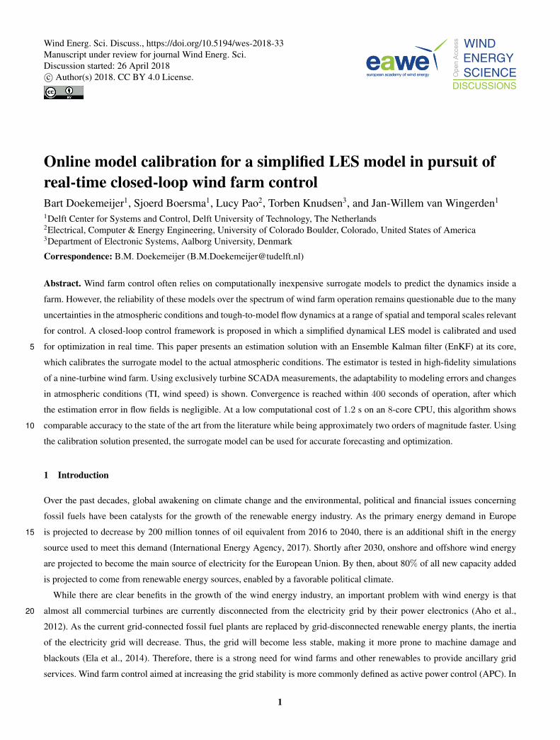
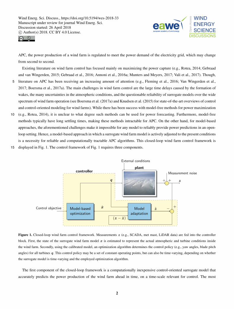


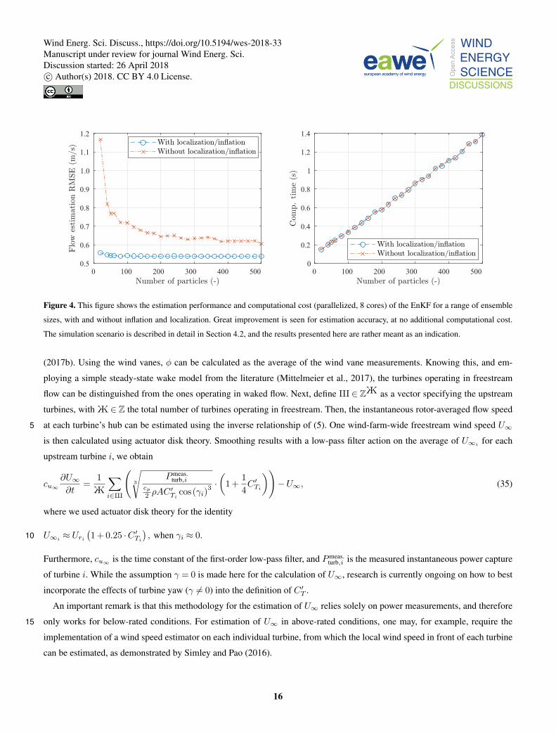


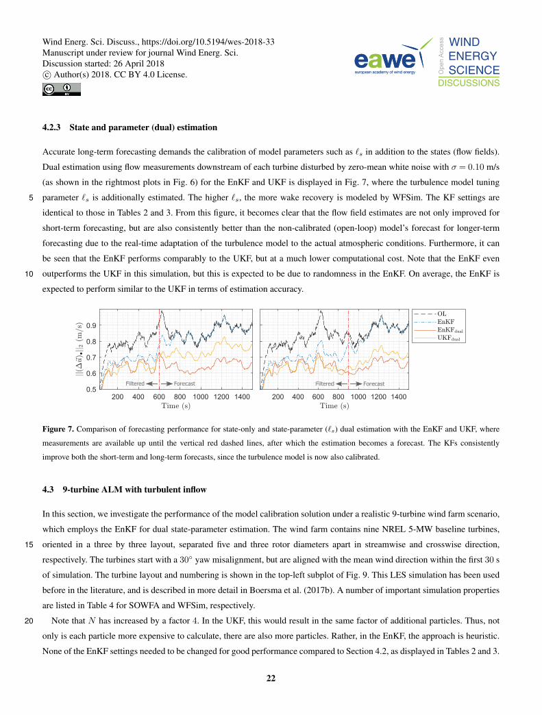


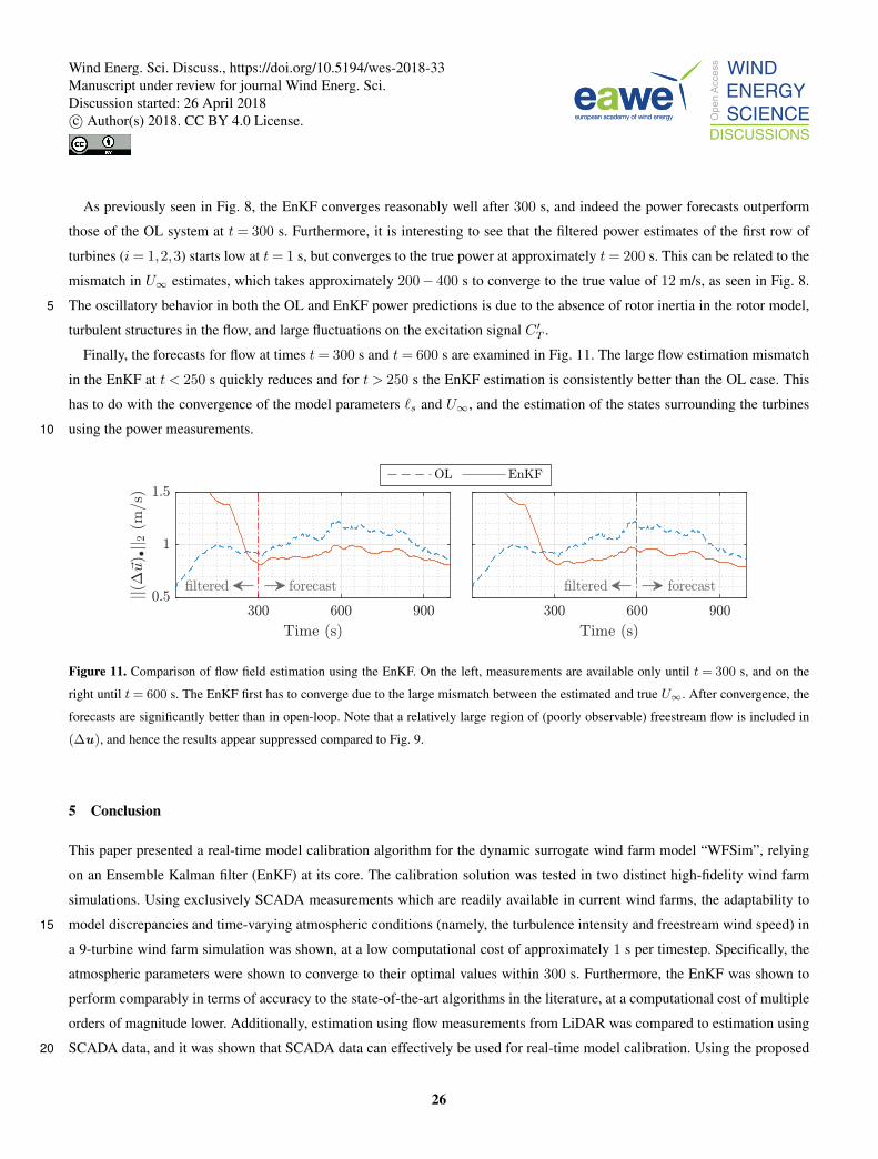


![[ VIP ] Simplied Methodology for Obtaining the Dynamic Model of Robot Manipualtors](https://static.documents.pub/doc/80x56/56d6bdca1a28ab30168f5b69/-vip-simplied-methodology-for-obtaining-the-dynamic-model-of-robot-manipualtors.jpg)


