Online Social Network Data Placement over Clouds

Online Social Network Data

Placement over Clouds

Dissertation

zur Erlangung des mathematisch-naturwissenschaftlichen Doktorgrades

"Doctor rerum naturalium"

der Georg-August-Universität Göttingen

in the PhD Programme in Computer Science (PCS)

of the Georg-August University School of Science (GAUSS)

vorgelegt von

Lei Jiao

aus Shaanxi, China

Göttingen, 2014

Thesis Committee

Prof. Dr. Xiaoming Fu

(Institute of Computer Science, University of Göttingen)

Prof. Jun Li, Ph.D.

(Department of Computer and Information Science,

University of Oregon, USA)

Prof. Dr. Dieter Hogrefe


Members of the Examination Board

Prof. Dr. Xiaoming Fu


Prof. Jun Li, Ph.D.

(Department of Computer and Information Science,

University of Oregon, USA)

Further Members of the Examination Board

Prof. Dr. Dieter Hogrefe


Prof. Dr. Carsten Damm


Prof. Dr. Konrad Rieck


Prof. Dr. Ramin Yahyapour

(GWDG; Institute of Computer Science, University of Göttingen)

Date of the Oral Examination: 10 July 2014

Abstract

Internet services today are often deployed and operated in data centers and

clouds; users access and use the services by connecting to such data centers from

their computing devices. For availability, fault tolerance, and proximities to users

at diverse regions, a service provider often needs to run the service at multiple

data centers or clouds that are distributed at different geographic locations, while

aiming to achieve many system objectives, e.g., a service provider may want to

reduce the money spent in using cloud resources, provide satisfactory service

quality, data availability to users, limit the carbon footprint of the service, and

so on. Inside a data center, a service provider is also concerned about some

system objectives, e.g., running a service across servers may need to diminish

the traffic that passes the oversubscribed core of the data center network.

A variety of system objectives can be addressed by carefully splitting and

placing data at different clouds or servers. For instance, different clouds may

charge different prices and emit different amounts of carbon for executing the

same workload; they also have different proximities to users. Different servers

inside a data center could reside at different positions in the data center network,

where the traffic between servers at a common rack does not affect the network

core but the traffic between servers at different racks may do. It is important for

a service provider to make right decisions about where to place users’ data over

a group of clouds or servers, as data placement influences system objectives.

This thesis investigates the data placement problem for the Online Social

Network (OSN) service, one of the most popular Internet services nowadays.

Data placement for the OSN service has many challenges. First of all, users’

data are interconnected. Ideally, the data of a user and the data of her friend

should be co-located at the same cloud or server so that the user can access all

the required data at a single site, saving any possible additional delay and traffic

going across cloud or sever boundaries. Secondly, the master-slave replication

complicates the data placement. A user may have a master replica that accepts

both read and write operations and several slave replicas that only accept read

operations; master and slave contribute differently to different system objectives

and the best locations to place them can also be different. Thirdly, if multiple

system objectives are considered, they are often intertwined, contradictory, and

cannot be optimized simultaneously. Saving expense needs data to be placed at

cheap clouds; reducing carbon prefers data to be placed at clouds with less carbon

i

Abstract

intensity; providing short latency requires data be placed close to users; data of

friends also need to be co-located. All these requirements cannot be met at the

same time and we desire a certain approach to seek trade-offs. On the other

hand, in the scenario inside a data center, the topology of data center networks

matters because, for different topologies, one often has different network traffic

performance goals and thus different optimal data placements.

Our contribution is that we study three different settings of the OSN data

placement problem by a combination of modeling, analysis, optimization, and

extensive simulations, capturing real-word scenarios in different contexts while

addressing all the aforementioned challenges. In the first problem, we optimize

the service provider’s monetary expense in using resources of geo-distributed

clouds with guaranteed service quality and data availability, while ensuring that

relevant users’ data are always co-located. Our proposed approach is based on

swapping the roles, master or slave, of a user’s data replicas. In the second prob-

lem, we optimize multiple system objectives of different dimensions altogether

when placing data across clouds by proposing a unified approach of decompos-

ing the problem into two subproblems of placing masters and slaves respectively.

We leverage the graph cuts technique to solve the master placement problem

and use a greedy approach to place slaves. In the third problem, focused on

the scenario inside a single data center, we encode different data center network

topologies and performance goals into our data placement problem and solve it

by borrowing our previous idea of swapping the roles of replicas and adapting

it to reaching network performance goals while doing role-swaps. To validate

our proposed approaches for each problem, we carry out extensive evaluations

using real-world large-scale data traces. We demonstrate that, compared with

state-of-the-art, de facto, and baseline methods, our approaches have significant

advantages in saving the monetary expense, optimizing multiple objectives, and

achieving various data center network performance goals, respectively. We also

have discussions on complexity, optimality, scalability, design alternatives, etc.

ii

Acknowledgements

I have been fortunate to work with many people, without whose help this thesis

would never have been possible. I owe tremendous thanks to them.

I give my deep appreciation to my advisor Prof. Dr. Xiaoming Fu. It was

his constant guidance, support, and encouragement that spurred me to pursue

research. His valuable assistance, suggestions, and feedback helped shape all my

research work these years.

I am greatly indebted to Prof. Jun Li, Ph.D., who co-advised my doctoral

study. He spent a lot of time revising, polishing, and improving almost every

single paper of mine. Without his patience and efforts, this thesis would not

have been what it is today.

My special gratitude goes to Dr. Wei Du. He had lots of insightful and

fruitful discussions with me on the details of my work. I learnt and benefited

hugely from our communications and collaboration.

I also thank Tianyin Xu and Dr. Yang Chen for their hands-on, useful advice.

My thanks in addition go to Prof. Dr. Dieter Hogrefe for being a member

of my thesis committee; I also thank him, Prof. Dr. Carsten Damm, Prof. Dr.

Konrad Rieck, and Prof. Dr. Ramin Yahyapour for serving as the examination

board for me. Their comments made this thesis better.

I owe a great deal to my family. Their unconditional and endless love and

support is always my motivation to go forward. To them I dedicate this thesis.

iii

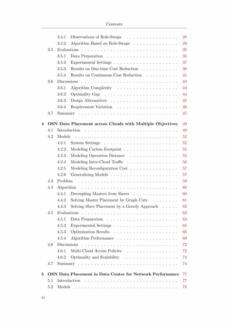
Contents

Abstract . . . . . . . . . . . . . . . . . . . . . . . . . . . . . . . . . . . i

Acknowledgements . . . . . . . . . . . . . . . . . . . . . . . . . . . . . iii

Contents . . . . . . . . . . . . . . . . . . . . . . . . . . . . . . . . . . . v

1 Introduction . . . . . . . . . . . . . . . . . . . . . . . . . . . . . . . 1

1.1 Problem . . . . . . . . . . . . . . . . . . . . . . . . . . . . . . . 1

1.2 Methodology . . . . . . . . . . . . . . . . . . . . . . . . . . . . . 3

1.3 Contributions . . . . . . . . . . . . . . . . . . . . . . . . . . . . 5

1.3.1 Saving Expense while Ensuring Social Locality . . . . . . 5

1.3.2 Addressing Multiple Objectives via Graph Cuts . . . . . 6

1.3.3 Achieving Data Center Network Performance Goals . . . 6

1.4 Deployment Considerations . . . . . . . . . . . . . . . . . . . . . 7

1.5 Thesis Organization . . . . . . . . . . . . . . . . . . . . . . . . . 7

2 Related Work . . . . . . . . . . . . . . . . . . . . . . . . . . . . . . 11

2.1 Placing OSN across Clouds . . . . . . . . . . . . . . . . . . . . . 11

2.2 Placing OSN across Servers . . . . . . . . . . . . . . . . . . . . . 12

2.3 Optimizing Cloud Services . . . . . . . . . . . . . . . . . . . . . 13

2.4 Graph Partitioning . . . . . . . . . . . . . . . . . . . . . . . . . 15

3 OSN Data Placement across Clouds with Minimal Expense . 17

3.1 Introduction . . . . . . . . . . . . . . . . . . . . . . . . . . . . . 17

3.2 Models . . . . . . . . . . . . . . . . . . . . . . . . . . . . . . . . 19

3.2.1 System Settings . . . . . . . . . . . . . . . . . . . . . . . 19

3.2.2 Modeling the Storage and the Inter-Cloud Traffic Cost . 20

3.2.3 Modeling the Redistribution Cost . . . . . . . . . . . . . 21

3.2.4 Approximating the Total Cost . . . . . . . . . . . . . . . 22

3.2.5 Modeling QoS and Data Availability . . . . . . . . . . . 24

3.3 Problem . . . . . . . . . . . . . . . . . . . . . . . . . . . . . . . 25

3.3.1 Problem Formulation . . . . . . . . . . . . . . . . . . . . 25

3.3.2 Contrast with Existing Problems . . . . . . . . . . . . . . 27

3.3.3 NP-Hardness Proof . . . . . . . . . . . . . . . . . . . . . 27

3.4 Algorithm . . . . . . . . . . . . . . . . . . . . . . . . . . . . . . 28

v

Contents

3.4.1 Observations of Role-Swaps . . . . . . . . . . . . . . . . 28

3.4.2 Algorithm Based on Role-Swaps . . . . . . . . . . . . . . 29

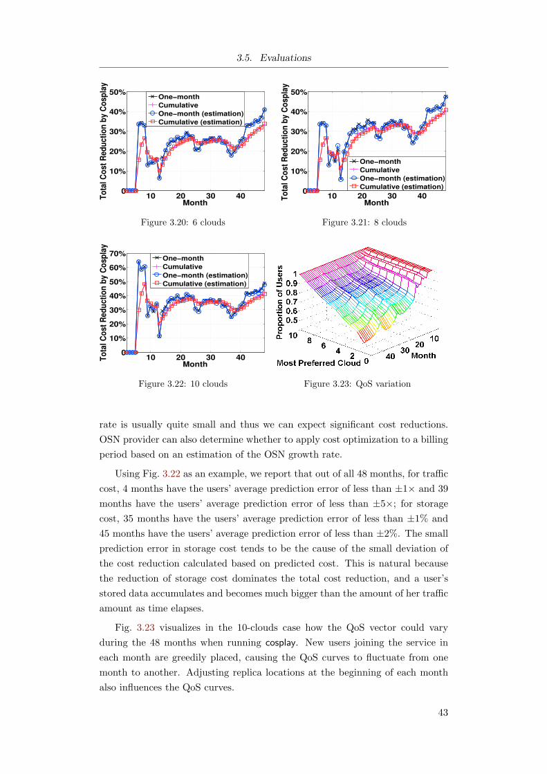
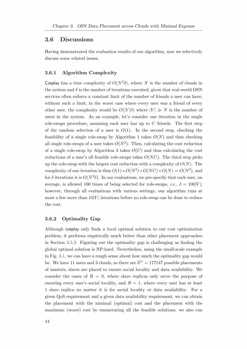
3.5 Evaluations . . . . . . . . . . . . . . . . . . . . . . . . . . . . . . 35

3.5.1 Data Preparation . . . . . . . . . . . . . . . . . . . . . . 35

3.5.2 Experimental Settings . . . . . . . . . . . . . . . . . . . . 37

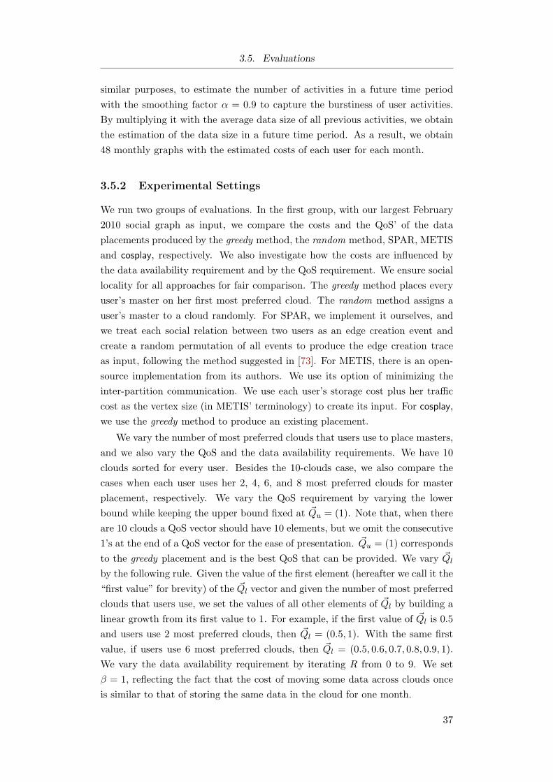
3.5.3 Results on One-time Cost Reduction . . . . . . . . . . . 38

3.5.4 Results on Continuous Cost Reduction . . . . . . . . . . 41

3.6 Discussions . . . . . . . . . . . . . . . . . . . . . . . . . . . . . . 44

3.6.1 Algorithm Complexity . . . . . . . . . . . . . . . . . . . 44

3.6.2 Optimality Gap . . . . . . . . . . . . . . . . . . . . . . . 44

3.6.3 Design Alternatives . . . . . . . . . . . . . . . . . . . . . 45

3.6.4 Requirement Variation . . . . . . . . . . . . . . . . . . . 46

3.7 Summary . . . . . . . . . . . . . . . . . . . . . . . . . . . . . . . 47

4 OSN Data Placement across Clouds with Multiple Objectives 49

4.1 Introduction . . . . . . . . . . . . . . . . . . . . . . . . . . . . . 49

4.2 Models . . . . . . . . . . . . . . . . . . . . . . . . . . . . . . . . 52

4.2.1 System Settings . . . . . . . . . . . . . . . . . . . . . . . 52

4.2.2 Modeling Carbon Footprint . . . . . . . . . . . . . . . . . 55

4.2.3 Modeling Operation Distance . . . . . . . . . . . . . . . 55

4.2.4 Modeling Inter-Cloud Traffic . . . . . . . . . . . . . . . . 56

4.2.5 Modeling Reconfiguration Cost . . . . . . . . . . . . . . . 57

4.2.6 Generalizing Models . . . . . . . . . . . . . . . . . . . . . 57

4.3 Problem . . . . . . . . . . . . . . . . . . . . . . . . . . . . . . . 59

4.4 Algorithm . . . . . . . . . . . . . . . . . . . . . . . . . . . . . . 60

4.4.1 Decoupling Masters from Slaves . . . . . . . . . . . . . . 60

4.4.2 Solving Master Placement by Graph Cuts . . . . . . . . 61

4.4.3 Solving Slave Placement by a Greedy Approach . . . . . 62

4.5 Evaluations . . . . . . . . . . . . . . . . . . . . . . . . . . . . . . 63

4.5.1 Data Preparation . . . . . . . . . . . . . . . . . . . . . . 63


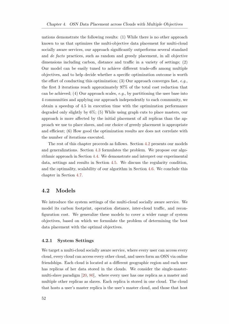
4.5.3 Optimization Results . . . . . . . . . . . . . . . . . . . . 66

4.5.4 Algorithm Performance . . . . . . . . . . . . . . . . . . . 69

4.6 Discussions . . . . . . . . . . . . . . . . . . . . . . . . . . . . . . 72

4.6.1 Multi-Cloud Access Policies . . . . . . . . . . . . . . . . 72

4.6.2 Optimality and Scalability . . . . . . . . . . . . . . . . . 74

4.7 Summary . . . . . . . . . . . . . . . . . . . . . . . . . . . . . . . 74

5 OSN Data Placement in Data Center for Network Performance 77

5.1 Introduction . . . . . . . . . . . . . . . . . . . . . . . . . . . . . 77

5.2 Models . . . . . . . . . . . . . . . . . . . . . . . . . . . . . . . . 78

vi

5.2.1 Revisiting Social Locality . . . . . . . . . . . . . . . . . . 79

5.2.2 Encoding Network Performance Goals . . . . . . . . . . . 79

5.3 Problem . . . . . . . . . . . . . . . . . . . . . . . . . . . . . . . 80

5.4 Algorithm . . . . . . . . . . . . . . . . . . . . . . . . . . . . . . 82

5.4.1 Achieving Performance Goals via Role-Swaps . . . . . . . 82

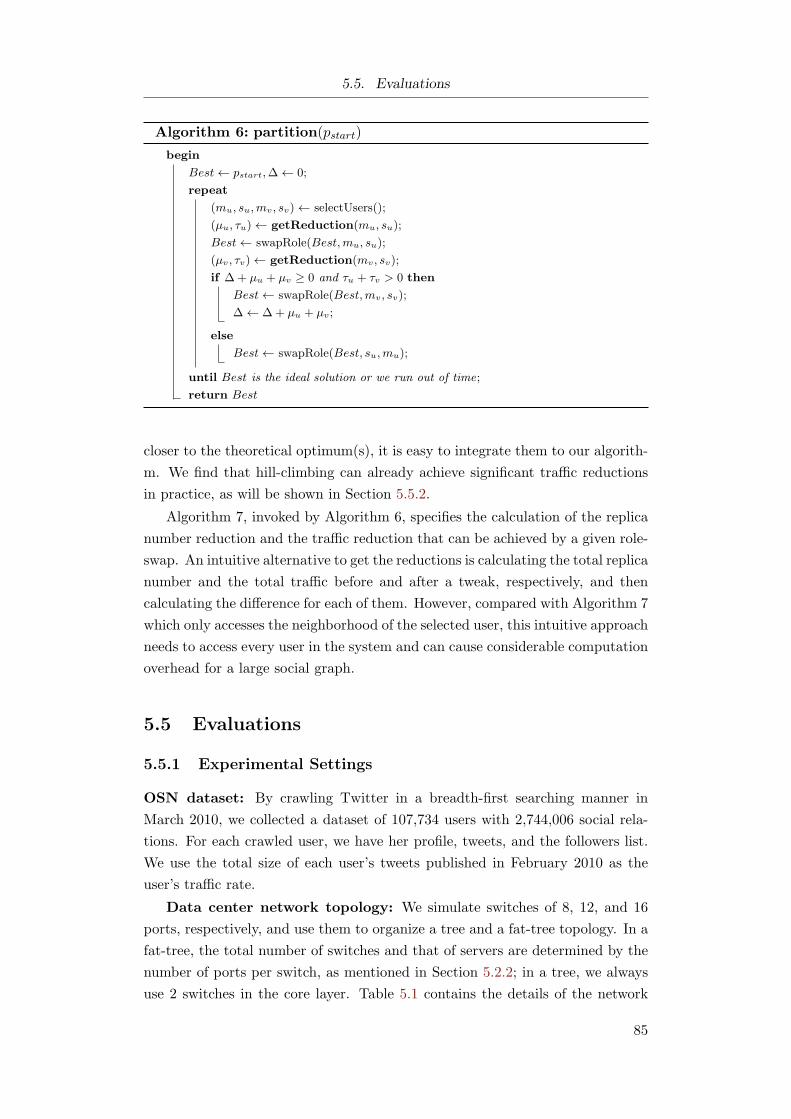
5.4.2 Traffic-Aware Partitioning Algorithm . . . . . . . . . . . 83

5.5 Evaluations . . . . . . . . . . . . . . . . . . . . . . . . . . . . . . 85


5.5.2 Evaluation Results . . . . . . . . . . . . . . . . . . . . . 86

5.6 Discussions . . . . . . . . . . . . . . . . . . . . . . . . . . . . . . 88

5.7 Summary . . . . . . . . . . . . . . . . . . . . . . . . . . . . . . . 88

6 Conclusion . . . . . . . . . . . . . . . . . . . . . . . . . . . . . . . . 91

6.1 Comparative Summary . . . . . . . . . . . . . . . . . . . . . . . 91

6.2 Future Work . . . . . . . . . . . . . . . . . . . . . . . . . . . . . 93

6.2.1 Data Placement vs. Request Distribution . . . . . . . . . 93

6.2.2 Online Optimization over Time . . . . . . . . . . . . . . 93

6.2.3 A Game Theoretic Perspective . . . . . . . . . . . . . . . 94

Bibliography . . . . . . . . . . . . . . . . . . . . . . . . . . . . . . . . . 97

vii

Chapter 1

Introduction

1.1 Problem

A large number of today’s Internet services are deployed and operated in data

centers [17, 23, 47, 89]. Users access and use the services by connecting to data

centers from their computers, mobile phones, or other devices. Data centers, the

service infrastructure, provide resources like computation, storage, and network.

Cloud can provide “Infrastructure-as-a-Service” [34, 66, 71, 83] so that service

providers do not have to build and maintain their own data centers; instead,

they deploy their services in the cloud, which are built and operated by cloud

providers, and pay for cloud resources that they use. A “cloud” here refers to a

special data center that uses dedicated software to virtualize its resources and

deliver them to customers. Running a service in the cloud has many advantages:

cloud resources are ready to consume, letting service providers focus on their

services rather than on building the service infrastructure which may not be their

competence; cloud resources are “infinite”, on demand, and can accommodate

the surges of user requests, making it easy to scale the service; cloud resources are

charged flexibly, “pay-as-you-go”, and can save the expenses of service providers.

No matter operating a service in one’s own data center or in the cloud, a

service provider often needs its service to span multiple geographic areas for the

purposes of availability, scalability, fault tolerance, and proximities to users at

diverse regions [50, 80, 93, 94], with concerns on several different aspects. For

instance, one may want to optimize the total monetary expense spent in using

resources of multiple clouds [92, 98], including the cost of running virtual ma-

chines, storing data, and the cost for the traffic between clouds and between

clouds and the users of the service, and so on. One may also want to provide

good service quality, such as short access latency [61, 95], and satisfactory data

availability [24, 49] to users. One may be even concerned about the carbon foot-

print of the service [58, 102], as carbon becomes an increasingly important issue

nowadays. Depending on the specific scenarios, the concerns can be different.

A range of such concerns can be addressed by appropriately choosing at which

data center or cloud to place which piece of data, given a group of candidate data

centers or clouds that reside at different locations [13, 16, 40, 77]. For example,

different clouds may charge different prices for consuming the same amount

of resources, have different proximities to users, and emit different amounts

1

Chapter 1. Introduction

of carbon for executing the same workload. Hence, data placement across the

clouds can influence the performance and various system objectives of the service.

Inside a data center, choosing at which server to place which piece of data

is also important. It is often not possible to host everything in a single server;

splitting data across servers, however, needs to meet various performance goal-

s [32, 72]. Different servers may reside at different positions in the data center

network. For example, the communication between some servers only passes one

switch because the servers are at a common rack; the communication between

some other servers may need to travel through more switches up to the core layer

of the data center network topology as they are at different racks. Data place-

ment in this case affects the paths that the inter-server communication travels

along and thus further affects the usage of network resources.

This thesis specifically investigates the problem of placing Online Social Net-

work (OSN) data both across multiple clouds or data centers, and across multiple

servers inside a data center. OSN services are undoubtedly among the most pop-

ular Internet services nowadays. Facebook had 1.28 billion monthly active users

as of March 31, 2014 [4]. Besides typical OSN services like Facebook and Twit-

ter, an important observation is that “social” is gradually becoming a universal

component of a large number of services, such as blogging, video sharing, and

others, all what we may call the “socially aware” services.

There are some critical challenges for placing the data of OSN or the socially

aware services over clouds and over servers inside a data center.

First of all, users of the OSN service are interconnected and the placements

of their data are interdependent [13, 35, 37, 72]. It is not that we choose the best

location for a user’s data, a cloud or a server, by considering the information of

this user alone, but that when placing a user’s data, we must also consider other

users who access such data. The feature of OSN services is letting users form

online friendships and communicate with one another, often by accessing the

data of others. Each user is not independent and cannot be treated separately

with regards to data placement. Ideally, for example, if the data of a user and

the data of her friends are always co-located at the same cloud or sever, a user

can access her friends’ data without going to another cloud or server, and thus

save any possible additional delay and traffic. This is unlike conventional web-

browsing services where users may not need to be jointly considered.

Secondly, the master-slave replication of users’ data complicates the place-

ment [28, 80]. It is a common practice that a service may maintain multiple

copies of a user’s data, where one copy may be the master replica and the oth-

ers are all slave replicas. When placing users’ data, we must determine where

to place each replica of each user. The difficulty is that different replicas serve

different purposes and contribute differently to various system objectives. For

example, a master replica accepts both read and write operations from either the

2

1.2. Methodology

user herself or her friends, while a slave replica accepts only read operations from

users; besides, writes to a master need to be propagated to the corresponding

slaves for consistency. The best location for a user’s master may be different

from that for a user’s slave; where to place each of a user’s salves is also an issue.

Thirdly, if multiple system objectives are considered altogether, they are

often intertwined, contradictory, and cannot be accommodated simultaneous-

ly [40, 99]. It is natural for a service provider to bear concerns from multiple

dimensions, for example, monetary expense, QoS, carbon emission, as stated

perviously. We cannot expect that a placement can address all such concerns to

the best. To save money, we like cheap clouds; to provide good QoS, we prefer

to place the data of a user at the cloud close to her; to make less carbon, we had

better use those with less carbon intensity; besides, we should not forget that

users’ data are interdependent. When the clouds that are chosen to address each

concern are different, as is often the case, we desire a certain approach to offer

the capability of seeking trade-offs among multiple objectives.

In fact, the challenges are not limited to what have been stated here. In

the wide-area multi-cloud scenario, we also need to consider how users access

the data [82]. For instance, if a piece of required data is not present at the

current cloud connected by a user, which other cloud with the required data

this user should access determines where the read workload is executed and the

corresponding carbon footprint is generated. In the local-area case inside a data

center, the topology of the data center network matters if one wants to use

data placement to dictate the network resource usage. In this thesis, we aim to

address all such challenges.

1.2 Methodology

We attack the OSN data placement problem via studying the following three

problem settings, corresponding to Chapter 3, Chapter 4, and Chapter 5, re-

spectively. Chapters 3 and 4 investigate OSN data placement across clouds,

and Chapter 5 investigates OSN data placement across servers inside a cloud.

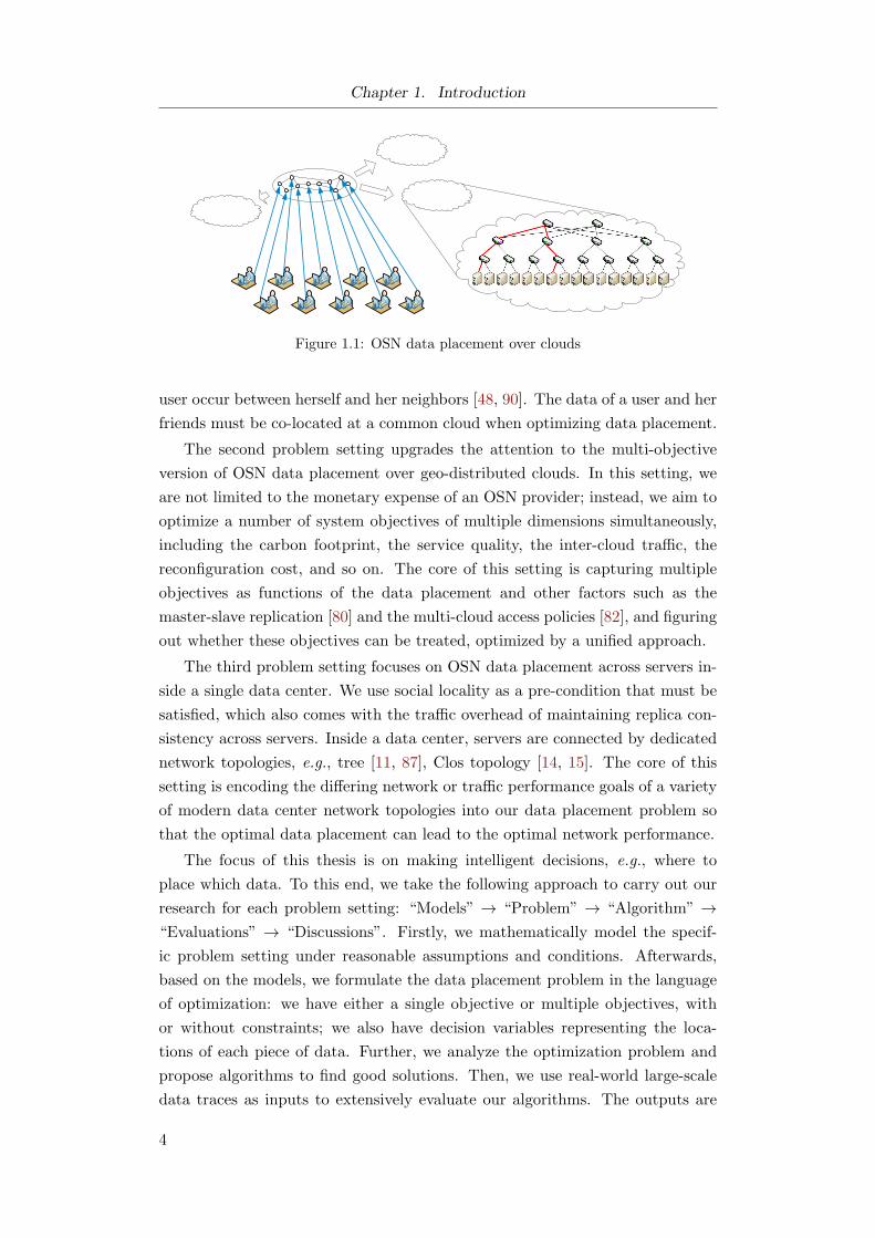
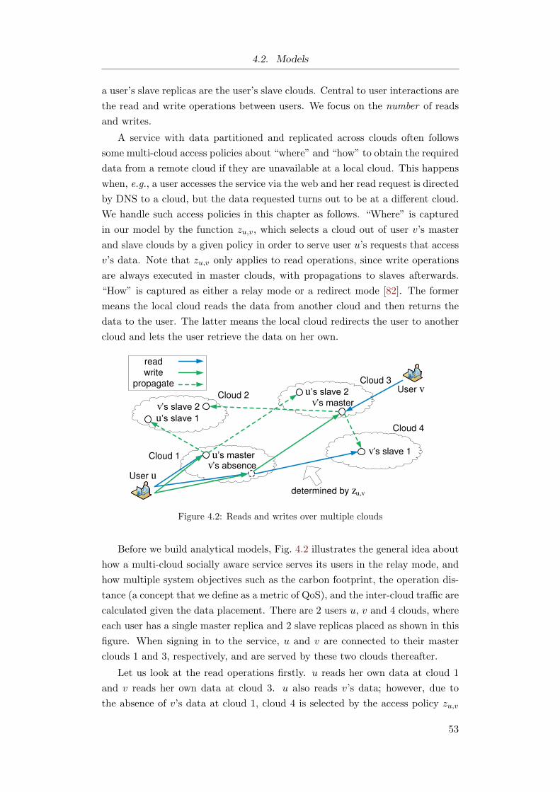
Fig. 1.1 is an overall picture of our work in this thesis. Users access their data

in the OSN service. An OSN provider firstly needs to determine how to dis-

tribute users’ data across multiple clouds, and then inside each cloud, it needs

to determine how to distribute users’ data across multiple servers.

The first problem setting aims to optimize the monetary expense that an

OSN provider spends in using resources of multiple geo-distributed clouds, while

providing satisfactory service quality and data availability to OSN users. In

addition to modeling various costs of a multi-cloud OSN, the QoS requirement,

and the data availability requirement, the core of this setting is ensuring for

every user the social locality [73, 81], the access pattern that most activities of a

3


Figure 1.1: OSN data placement over clouds

user occur between herself and her neighbors [48, 90]. The data of a user and her

friends must be co-located at a common cloud when optimizing data placement.

The second problem setting upgrades the attention to the multi-objective

version of OSN data placement over geo-distributed clouds. In this setting, we

are not limited to the monetary expense of an OSN provider; instead, we aim to

optimize a number of system objectives of multiple dimensions simultaneously,

including the carbon footprint, the service quality, the inter-cloud traffic, the

reconfiguration cost, and so on. The core of this setting is capturing multiple

objectives as functions of the data placement and other factors such as the

master-slave replication [80] and the multi-cloud access policies [82], and figuring

out whether these objectives can be treated, optimized by a unified approach.

The third problem setting focuses on OSN data placement across servers in-

side a single data center. We use social locality as a pre-condition that must be

satisfied, which also comes with the traffic overhead of maintaining replica con-

sistency across servers. Inside a data center, servers are connected by dedicated

network topologies, e.g., tree [11, 87], Clos topology [14, 15]. The core of this

setting is encoding the differing network or traffic performance goals of a variety

of modern data center network topologies into our data placement problem so

that the optimal data placement can lead to the optimal network performance.

The focus of this thesis is on making intelligent decisions, e.g., where to

place which data. To this end, we take the following approach to carry out our

research for each problem setting: “Models” → “Problem” → “Algorithm” →

“Evaluations” → “Discussions”. Firstly, we mathematically model the specif-

ic problem setting under reasonable assumptions and conditions. Afterwards,

based on the models, we formulate the data placement problem in the language

of optimization: we have either a single objective or multiple objectives, with

or without constraints; we also have decision variables representing the loca-

tions of each piece of data. Further, we analyze the optimization problem and

propose algorithms to find good solutions. Then, we use real-world large-scale

data traces as inputs to extensively evaluate our algorithms. The outputs are

4

1.3. Contributions

compared with those produced by other state-of-the-art, de facto, or baseline

approaches. We interpret and explain the evaluation results. Finally, we discuss

the various aspects such as complexity, optimality, scalability, design alterna-

tives, and so on. We either do additional evaluations to assist our discussions or

conduct discussions only based on our models.

1.3 Contributions

We study the three different problem settings as stated previously, capturing

real-world scenarios in different contexts, by a combination of modeling, analysis,

optimization, and simulation.

1.3.1 Saving Expense while Ensuring Social Locality

In the first problem setting, we model the cost of an OSN as the objective,

and model the QoS and the data availability requirements as the constraints of

the data placement optimization problem. Our cost model identifies different

types of costs associated with a multi-cloud OSN, including the storage cost

and the inter-cloud traffic cost incurred by storing and maintaining users’ data

in the clouds, as well as the redistribution cost incurred by our optimization

mechanism itself. All kinds of costs ensure the social locality [73, 81] for every

user as a premise. Translated into the master-slave paradigm that we consider,

it means that a user’s every neighbor must have either a master replica or a slave

replica at the cloud that hosts the user’s own master replica. Our QoS model

links the QoS of the OSN service with the locations of all users’ master replicas

over clouds. Our data availability model relates with the minimum number of

replicas of each user. We prove the NP-hardness of the optimization problem.

Our core contribution is an algorithm named cosplay that is based on our ob-

servations that swapping the roles (i.e., master or slave) of a user’s data replicas

on different clouds can not only lead to possible cost reduction, but also serve

as an elegant approach to ensuring QoS and maintaining data availability. We

carry out extensive experiments by distributing a real-world geo-social Twitter

dataset of 321,505 users with 3,437,409 social relations over 10 clouds all across

the US in a variety of settings. Our results demonstrate that, while always en-

suring the QoS and the data availability as required, cosplay can reduce much

more one-time cost than the state of the arts, and it can also significantly reduce

the accumulative cost when continuously evaluated over 48 months, with OSN

dynamics comparable to real-world cases. We analyze that cosplay has quite a

moderate complexity, and show that cosplay tends to produce data placements

within a reasonably good optimality gap towards the global optimum. We also

discuss other possible design alternatives and extended use cases.

5


1.3.2 Addressing Multiple Objectives via Graph Cuts

In the second problem setting, we allow every user having one master replica and

a fixed number of slave replicas, based on which we model various system objec-

tives including the carbon footprint, the service quality, the inter-cloud traffic,

as well as the reconfiguration cost incurred by changing one data placement to

another, considering the multi-cloud access policies. The big change compared

with the first problem setting is that we give up ensuring social locality for every

user. A possible consequence of this change is that we find all the models of

system objectives composed of one or both of the two parts: a unary term that

only depends on the locations of a single user’s replicas and a pairwise term that

depends on the locations of the replicas of a pair of users. Besides, our models

can be generalized to cover a wide range of other system objectives.

Our core contribution here is a unified approach to optimize the multiple

objectives. We propose to decompose our original data placement problem into

two simpler subproblems and solve them alternately in multiple rounds: in one

problem, given the locations of all slaves, we identify the optimal locations of

all masters by iteratively invoking the graph cuts technique [25, 26, 56]; in the

other subproblem, we place all slaves given the locations of all masters, where

we find that the optimal locations of each user’s slaves are independent and

a greedy method that takes account of all objectives can be sufficient. We

conduct evaluations using a real-world dataset of 107,734 users interacting over

2,744,006 social relations, and place these users’ data over 10 clouds all across

the US. We demonstrate results that are significantly better than standard and

de facto methods in all objectives, and also show that our approach is capable of

exploring trade-offs among objectives, converges fast, and scales to a huge user

base. While proposing graph cuts to address master replicas placement, we find

that different initial placements of all replicas and different methods of placing

slave replicas can influence the optimization results to different extents, shedding

light on how to better control our algorithm to achieve desired optimizations.

1.3.3 Achieving Data Center Network Performance Goals

In the third problem setting, we consider a diversity of modern data center

network topologies inside the data center, identify the different network or traffic

performance goals, and encode these goals into our data placement optimization

problem. While a general network performance goal would be minimizing the

sum of the amount of traffic passing every router, in the conventional three-

layer tree topology with heavy oversubscription minimizing the amount of traffic

passing the core-layer routers seems more important. Here in this setting we still

ensure social locality, which comes with the storage overhead of slave replicas

and the network overhead of the traffic of maintaining replica consistency across

6

1.4. Deployment Considerations

servers. We aim to align such traffic with various network performance goals by

carefully selecting servers to place each user’s master and slave replicas, while

guaranteeing that the storage overhead does not increase.

Our contribution here is borrowing our previous idea of swapping the roles

of data replicas and adapting it to achieving network performance goals during

role-swaps. Through evaluations with a large-scale, real-world Twitter trace, we

show that in a variety of data center network topologies with a varying number

of servers, compared with state-of-the-art algorithms, our algorithm significantly

reduces traffic, achieving various network performance goals without deteriorat-

ing the load balance among servers and causing extra replication overhead.

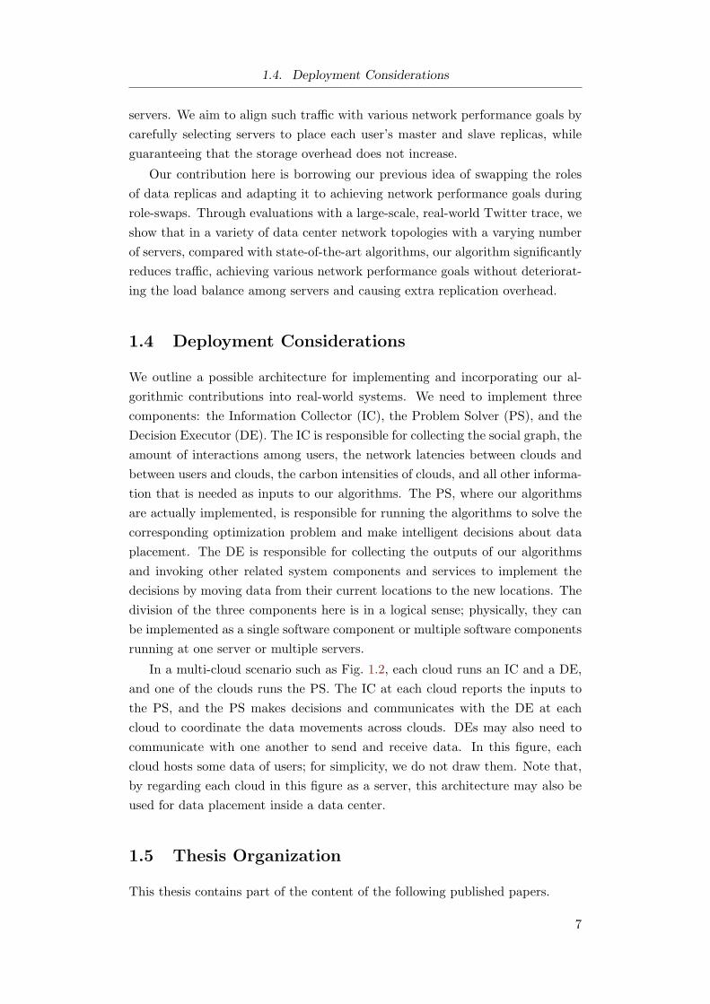
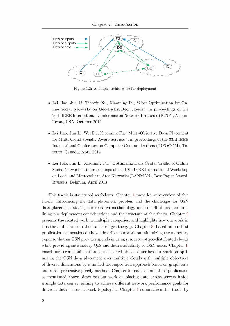
1.4 Deployment Considerations

We outline a possible architecture for implementing and incorporating our al-

gorithmic contributions into real-world systems. We need to implement three

components: the Information Collector (IC), the Problem Solver (PS), and the

Decision Executor (DE). The IC is responsible for collecting the social graph, the

amount of interactions among users, the network latencies between clouds and

between users and clouds, the carbon intensities of clouds, and all other informa-

tion that is needed as inputs to our algorithms. The PS, where our algorithms

are actually implemented, is responsible for running the algorithms to solve the

corresponding optimization problem and make intelligent decisions about data

placement. The DE is responsible for collecting the outputs of our algorithms

and invoking other related system components and services to implement the

decisions by moving data from their current locations to the new locations. The

division of the three components here is in a logical sense; physically, they can

be implemented as a single software component or multiple software components

running at one server or multiple servers.

In a multi-cloud scenario such as Fig. 1.2, each cloud runs an IC and a DE,

and one of the clouds runs the PS. The IC at each cloud reports the inputs to

the PS, and the PS makes decisions and communicates with the DE at each

cloud to coordinate the data movements across clouds. DEs may also need to

communicate with one another to send and receive data. In this figure, each

cloud hosts some data of users; for simplicity, we do not draw them. Note that,

by regarding each cloud in this figure as a server, this architecture may also be

used for data placement inside a data center.

1.5 Thesis Organization

This thesis contains part of the content of the following published papers.

7


Flow of inputs

Flow of outputs

Flow of data

DE

DE

DE

PS

IC

IC

IC

Figure 1.2: A simple architecture for deployment

• Lei Jiao, Jun Li, Tianyin Xu, Xiaoming Fu, “Cost Optimization for On-

line Social Networks on Geo-Distributed Clouds”, in proceedings of the

20th IEEE International Conference on Network Protocols (ICNP), Austin,

Texas, USA, October 2012

• Lei Jiao, Jun Li, Wei Du, Xiaoming Fu, “Multi-Objective Data Placement

for Multi-Cloud Socially Aware Services”, in proceedings of the 33rd IEEE

International Conference on Computer Communications (INFOCOM), To-

ronto, Canada, April 2014

• Lei Jiao, Jun Li, Xiaoming Fu, “Optimizing Data Center Traffic of Online

Social Networks”, in proceedings of the 19th IEEE International Workshop

on Local and Metropolitan Area Networks (LANMAN), Best Paper Award,

Brussels, Belgium, April 2013

This thesis is structured as follows. Chapter 1 provides an overview of this

thesis: introducing the data placement problem and the challenges for OSN

data placement, stating our research methodology and contributions, and out-

lining our deployment considerations and the structure of this thesis. Chapter 2

presents the related work in multiple categories, and highlights how our work in

this thesis differs from them and bridges the gap. Chapter 3, based on our first

publication as mentioned above, describes our work on minimizing the monetary

expense that an OSN provider spends in using resources of geo-distributed clouds

while providing satisfactory QoS and data availability to OSN users. Chapter 4,

based our second publication as mentioned above, describes our work on opti-

mizing the OSN data placement over multiple clouds with multiple objectives

of diverse dimensions by a unified decomposition approach based on graph cuts

and a comprehensive greedy method. Chapter 5, based on our third publication

as mentioned above, describes our work on placing data across servers inside

a single data center, aiming to achieve different network performance goals for

different data center network topologies. Chapter 6 summarizes this thesis by

8

1.5. Thesis Organization

comparing our studies in Chapters 3, 4 and 5 with one another, and finally shares

some of our thoughts on the future work.

9

Chapter 2

Related Work

We discuss existing work in four categories, and for each category, we summarize

how the work fails to address the challenges that are faced by placing OSN over

clouds, and highlight how our work in this thesis bridges the gap. The first two

categories are on placing and optimizing the data of OSN and social media across

clouds and across servers inside a cloud, which may be the work most related to

ours. The third category is about socially oblivious cloud services, demonstrating

what can be some important performance metrics of cloud services and how they

can be optimized. The last category, from a graph theory perspective, introduces

the study of graph partitioning and repartitioning problems that seem similar

to our problems of splitting and replicating OSN.

2.1 Placing OSN across Clouds

The multi-cloud or multi-data-center platform is promising for deploying and op-

erating OSN and socially aware services. A branch of existing work investigates

the challenges and opportunities towards this direction.

Liu et al. [60] focused on the inter-data-center communication of the OSN

service. Maintaining a replica of a remote user’s data at a local data center

reduced the inter-data-center read operations as local users could access such

data without going to remote data centers; however, this replica at the local

data center needed to be updated for consistency with remote replicas and thus

incurred the inter-data-center update operations. The authors proposed to repli-

cate across data centers only the data of the users selected by jointly considering

the read and the update rates in order to ensure that a replica could always

reduce the total inter-data-center communication.

Wittie et al. [91] claimed that Facebook had slow response to users outside

US and Internet bandwidth was wasted when users worldwide requested the

same content. The authors found that the slow response was caused by the

multiple round trips of Facebook communication protocols as well as the high

network latency between users and Facebook US data centers; they also observed

that most communications were among users within the same geographic region.

The authors proposed to use local servers as TCP proxies and caching servers to

improve service responsiveness and efficiency, focusing on the interplay between

user behavior, OSN mechanisms, and network characteristics.

11

Chapter 2. Related Work

Wu et al. [92] advocated using geo-distributed clouds for scaling the social

media streaming service. However, the challenges remained for storing and mi-

grating media data dynamically in the clouds for timely response and moderate

expense. To address such challenges, the authors proposed a set of algorithms

that were able to do online data migration and request distribution over consec-

utive time periods based on Lyapunov optimization techniques. They predicted

the user demands by exploiting the social influence among users; leveraging the

predicted information, their algorithms could also adjust the online optimization

result towards the offline optimum.

Wang et al. [86] targeted social applications which often had a workflow

of “collection” → “processing” → “distribution”. The authors proposed local

processing, which collected and processed user-generated content at local cloud-

s, and global distribution, which delivered processed content to users via geo-

distributed clouds, as a new principle to deploy social applications across clouds,

and designed protocols to connect these two components. They modeled and

solved optimization problems to determine computation allocation and content

replication across clouds, and built prototypes in real-world clouds to verify the

advantages of their design.

The work in this category focuses on the performance of OSN services [60,

91] and social applications [86], and the monetary expense of provisioning and

scaling social media in the clouds [92]. Our work in this thesis investigates

the monetary expense of the OSN service with its QoS and data availability

requirements, as well as the many other facets of the OSN performance over

clouds. To the best of our knowledge, we are the first to include the carbon

footprint of OSN services into consideration, with a complex trade-off among a

large variety of related factors such as QoS and inter-cloud traffic. In addition to

the generality of our models that can capture a diversity of performance metrics

and the uniqueness of our proposed algorithmic approach, we investigate this

complicated joint optimization problem in the context of master-slave replication

while accommodating different multi-cloud access policies.

2.2 Placing OSN across Servers

At a single site, how to partition and replicate the data of OSN and socially

aware services across servers remains another important problem. A body of

existing literature tackles this scenario.

OSN services often adopt distributed hashing to partition the data across

servers [7, 57], which can lead to poor performance such as unpredictable re-

sponse time due to the inter-server multi-get operations, and the response time

is determined by the server with the highest latency. To address this problem,

recent work proposed to eliminate the inter-server multi-get operations by main-

12

2.3. Optimizing Cloud Services

taining social locality, i.e., replicating friends across servers [72, 81] so that all

friends of a user could be accessed at a single server. SPAR [72] minimized the

total number of slave replicas while maintaining social locality for every user

and balancing the number of master replicas in each partition. S-CLONE [81]

maximized the number of users whose social locality could be maintained given

a fixed number of replicas for each user. Another approach [30] to tackle the

same problem explored self-similarities, a feature that was found in OSN inter-

actions and did not exist in OSN social relations. Self-similarity was known as

a driving force to minimize the dissipation of cost/energy in dynamic process.

The authors argued that placing users in the same self-similar subtree at the

same server minimized the inter-server communication.

Carrasco et al. [27] noticed that an OSN user’s queries often only cared

about the most recent messages of friends, and thus dividing messages according

to time stamps and placing those within a particular time range at a particular

server had far less storage overhead than partitioning messages only based on

OSN friendships. Partitioning along the time dimension could also serve as an

approach to optimize OSN performance.

Cheng et al. [31] considered partitioning social media content across servers.

The authors found that when doing such partitioning, not only the social rela-

tions should be considered, one also needed to consider the user access patterns

to each media file otherwise the viewing workload at each server could be skewed.

The authors formulated an optimization problem and solved it to preserve social

relations and to balance the workload among servers.

The work in this category is mainly on OSN and social media placement

optimization across servers at a single site. All such existing work cares more

often the server performance, and very little has been done on the network

performance. The root cause is that they essentially target a server cluster envi-

ronment, instead of a data center environment where the network performance

also needs considerable attention. Our work in this thesis identifies the network

performance goals for different data center networks, captures and encodes them

into our optimization problem. We propose a unified algorithm to place OSN

data across servers to optimize a diversity of such goals while maintaining social

locality. Our work is done in a way that we optimize network performance with-

out hurting server performance, i.e., without affecting the existing load balance

among servers and increasing the total replication overhead.

2.3 Optimizing Cloud Services

There exists rich research work on optimizing cloud services. Besides convention-

al performance metrics such as service latency, energy and carbon increasingly

becomes an important concern of optimization in recent years.

13

Chapter 2. Related Work

Qureshi et al. [74] might be the first to propose to exploit the difference of

electricity prices for clouds at different geo-locations. Electricity prices exhibited

both temporal and geographic variations due to various reasons such as region-

al demand differences, transmission inefficiencies, and diversities of generation

sources. Distributing requests to adjust the workload of each cloud could thus

lead to significant monetary savings for the total electric bills of all the clouds.

The authors also used bandwidth and performance as constraints.

Rao et al. [76] further observed that data centers could consume electrici-

ty from multiple markets: some US regions had wholesale electricity markets

where electricity prices might vary on an hourly or a 15-minute basis while the

prices in other regions without wholesale markets could remain unchanged for

a longer time period. The authors proposed to leverage both the market-based

and the location-based price differences to minimize the total electric bill while

guaranteeing the service delay captured by a queueing model.

Le et al. [58] studied the multi-data-center energy expense problem in a d-

ifferent setting. The authors argued that the brown energy, i.e., which was

produced by coal, should be capped and the green energy, i.e., which was pro-

duced by wind, water, etc., should be explored. Their work proposed a model

framework to capture the energy cost of services in the presence of brown energy

caps, data centers that could use green energy, and multiple electricity prices

and carbon markets. The authors minimized the energy cost by distributing

requests among data centers properly while abiding by service level agreements.

Xu et al. [95] jointly optimized the electricity cost and the bandwidth cost of

geo-distributed data centers. Electricity cost could be optimized via distributing

requests to data centers as stated previously. There was also room for bandwidth

cost optimization. Nowadays a data center often connected to multiple ISPs

simultaneously and a request, once processed at a data center, needed to be

routed back to the user via one of the available ISP links which often had different

prices. To exploit both price differences of electricity and bandwidth, the authors

modeled an optimization problem and solved it by a distributed algorithm.

Gao et al. [40], to the best of our knowledge, did the only work so far of

optimizing multiple dimensions of system objectives of distributed data centers

or clouds. The authors optimized carbon footprint, electricity cost, and access

latency through proper request distribution and content placement across data

centers. They proposed an optimization framework that allowed data center op-

erators to navigate the trade-offs among the three dimensions; they also studied

using their framework to do carbon-aware data center upgrades. A heuristic was

also available to achieve approximate solutions at a faster speed.

Besides electricity and carbon, a substantial body of literatures studies cloud

resource pricing [78] and allocation [54], as well as a range of other related issues

in the cloud scenario. We are not going into further details here.

14

2.4. Graph Partitioning

This category of work targets conventional and socially oblivious services.

Except [40], they often assume full data replication across data centers; even [40]

still cannot serve our purpose. The existing work does not address (1) social

relations and user interactions, (2) writes to contents and the maintenance of

replica consistency, (3) inter-cloud operations that contribute to QoS and inter-

cloud traffic, and (4) the master-slave replication that is widely used in reality,

and thus falls short in the problem space in the first place. In contrast, our

work in this thesis captures all such particular features in the context of socially

aware services and provides trade-offs among a wide range of system performance

metrics via our generalized model framework and a unified algorithmic approach.

2.4 Graph Partitioning

In the last part of this related work section, we briefly introduce the existing

study of graph partitioning and repartitioning problems. Conventionally, such

problems are studied from a graph theoretic and algorithmic perspective.

Graph partitioning aims to divide a weighted graph into a specified number of

partitions in order to minimize either the weights of edges that straddle partitions

or the inter-partition communication while balancing the weights of vertices

in each partition [12]; graph repartitioning additionally considers the existing

partitioning, and pursues the same objective as graph partitioning while also

minimizing the migration costs [79]. State-of-the-art algorithms and solutions

to such problems include METIS [53] and Scotch [70]. We take METIS here as

an example. METIS is a multi-level partitioning algorithm that is composed of

three phases: the coarsening phase, the partitioning phase, and the uncoarsening

phase. In the coarsening phase, vertices are merged iteratively dictated by some

rules and thus the size of the original graph becomes smaller and smaller. In

the partitioning phase, the smallest graph is partitioned. In the uncoarsening

phase, the partitioned graph is projected back to finer graphs iteratively and the

partitioning is also refined following some algorithms until one gets the finest,

original graph. There are many of such merging rules and refining algorithms

that one can consider for a specific instance of a graph partitioning problem.

The problems we study in this thesis have some fundamental differences from

the classic graph partitioning and repartitioning problems. Classic problems han-

dle weighed graphs and have no notion of social locality, QoS, data availability,

carbon, data center network topologies, etc., which makes their algorithms inap-

plicable to our cases, e.g., minimizing the total inter-server communication does

not necessarily minimize the traffic traveling via the core-layer switches or the

total traffic perceived by every switch, nor the carbon footprint and the access

latency. To solve problems that capture such concerns, in this thesis, we propose

novel algorithms based on swapping the roles of data replicas and graph cuts.

15

Chapter 3

OSN Data Placement across

Clouds with Minimal Expense

3.1 Introduction

Internet services today are experiencing two remarkable changes. One is the

unprecedented popularity of Online Social Networks (OSNs), where users build

social relationships, and create and share contents with one another. The oth-

er is the rise of clouds. Often spanning multiple geographic locations, clouds

provide an important platform for deploying distributed online services. Inter-

estingly, these two changes tend to be combined. While OSN services often have

a very large user base and need to scale to meet demands of users worldwide,

geo-distributed clouds that provide Infrastructure-as-a-Service can match this

need seamlessly, further with tremendous resource and cost efficiency advan-

tages: infinite on-demand cloud resources can accommodate the surges of user

requests; flexible pay-as-you-go charging schemes can save the investments of ser-

vice providers; and cloud infrastructures also free service providers from building

and operating ones’ own data centers. Indeed, a number of OSN services are

increasingly deployed on clouds, e.g., Sonico, CozyCot, and Lifeplat [2].

Migrating OSN services towards geographically distributed clouds must rec-

oncile the needs from several different aspects. First, OSN providers want to

optimize the monetary cost spent in using cloud resources. For instance, they

may wish to minimize the storage cost when replicating users’ data at more than

one cloud, or minimize the inter-cloud communication cost when users at one

cloud have to request the data of others that are hosted at a different cloud.

Moreover, OSN providers hope to provide OSN users with satisfactory quality of

service (QoS). To this end, they may want a user’s data and those of her friends

to be accessible from the cloud closest to the user, for example. Last but not

least, OSN providers may also be concerned of data availability, e.g., ensuring

the number of users’ data replicas to be no fewer than a specified threshold across

clouds. Addressing all such needs of cost, QoS, and data availability is further

complicated by the fact that an OSN continuously experiences dynamics, e.g.,

new users join, old users leave, and the social relations also vary.

Existing work on OSN service provisioning either pursues the least cost at

17

Chapter 3. OSN Data Placement across Clouds with Minimal Expense

a single site without the QoS concern as in the geo-distribution case [73, 81],

or aims at the least inter-data-center traffic in the case of multiple data centers

without considering other dimensions of the service [60], e.g., data availability.

More importantly, the models in all such work do not capture the monetary cost

of resource usage and thus cannot fit the cloud scenario. There are some work

on cloud-based social video [86, 92], focusing on leveraging online social rela-

tionships to improve video distribution, however still leaving a gap towards the

OSN service; most optimization research on multi-cloud and multi-data-center

services are not for OSN [13, 54, 78, 95]. They do not capture the OSN features

such as social relationships and user interactions, neither can their models be

applicable to OSN services.

In this chapter, we therefore study the problem of optimizing the monetary

cost of the dynamic, multi-cloud-based OSN, while ensuring its QoS and data

availability as required.

We first model the cost, the QoS, and the data availability of the OSN service

upon clouds. Our cost model identifies different types of costs associated with

multi-cloud OSN while capturing social locality [73, 81], an important feature

of the OSN service that most activities of a user occur between herself and

her neighbors. Guided by existing research on OSN growth and our analysis

of real-world OSN dynamics, our model approximates the total cost of OSN

over consecutive time periods when the OSN is large in user population but

moderate in growth, enabling us to achieve the optimization of the total cost by

independently optimizing the cost of each period. Our QoS model links the QoS

with OSN users’ data locations among clouds. For every user, all clouds available

are sorted in terms of a certain quality metric (e.g., access latency); therefore

every user can have the most preferred cloud, the second most preferred cloud,

and so on. The QoS of the OSN service is better if more users have their data

hosted on clouds of a higher preference. Our data availability model relates with

the minimum number of replicas maintained by each OSN user.

We then base on these models to formulate the cost optimization problem

which considers QoS and data availability requirements. We prove the NP-

hardness of our problem. We propose an algorithm named cosplay based on

our observations that swapping the roles (i.e., master or slave) of a user’s data

replicas on different clouds can not only lead to possible cost reduction, but also

serve as an elegant approach to ensuring QoS and maintaining data availability.

Compared with existing approaches, cosplay reduces cost significantly and finds a

substantially good solution of the cost optimization problem, while guaranteeing

all requirements are satisfied. Furthermore, not only can cosplay reduce the one-

time cost for a cloud-based OSN service, by estimating the heavy-tailed OSN

activities [21, 84] during runtime, it can also solve a series of instances of the

cost optimization problem and thus minimize the aggregated cost over time.

18

3.2. Models

We further carry out extensive experiments. We distribute a real-world geo-

social Twitter dataset of 321,505 users with 3,437,409 social relations over 10

clouds all across the US in a variety of settings. Compared with existing alter-

natives, including some straightforward methods such as the greedy placement

(the common practice of many online services [80, 82]), the random placement

(the de facto standard of data placement in distributed DBMS such as MySQL

and Cassandra [57]), and some state-of-the-art algorithms such as SPAR [73]

and METIS [53], cosplay produces better data placements. While meeting all

requirements, it can reduce the one-time cost by up to about 70%. Further, over

48 consecutive months with OSN dynamics comparable to real-world cases, com-

pared with the greedy placement, continuously applying cosplay can reduce the

accumulative cost by more than 40%. Our evaluations also demonstrate quanti-

tatively that the trade-off among cost, QoS, and data availability is complex, and

an OSN provider may have to try cosplay around all the three dimensions. For

instance, according to our results, the benefits of cost reduction decline when the

requirement for data availability is higher, whereas the QoS requirement does

not always influence the amount of cost that can be saved.

The remainder of this chapter is structured as follows. Section 3.2 describes

our models of the cost, QoS, and data availability of the OSN service over multi-

ple clouds. Section 3.3 formulates the cost optimization problem. Section 3.4 e-

laborates our cosplay algorithm, as well as our considerations and insights behind.

Section 3.5 demonstrates and interprets our evaluations. Section 3.6 discusses

some related issues such as complexity and optimality. Section 3.7 concludes.

3.2 Models

Targeting the OSN service over multiple clouds, we begin with identifying the

types of costs related to cloud resource utilization: the storage cost for storing

users’ data, the inter-cloud traffic cost for synchronizing data replicas across

clouds, the redistribution cost incurred by the cost optimization mechanism it-

self, and some underlying maintenance cost for accommodating OSN dynamics.

We discuss and approximate the total cost of the multi-cloud OSN over time.

Afterwards, we propose a vector model to capture the QoS of the OSN service,

show the features of this model, and demonstrate its usage. Finally, we model

the OSN data availability requirement by linking it with the minimum number

of each user’s data replicas.

3.2.1 System Settings

Clouds and OSN users are all geographically distributed. Without loss of gener-

ality, we consider the single-master-multi-slave paradigm [20, 80]: each user has

19


only one master replica and several slave replicas of her data, where each replica

is hosted at a different cloud. When signing in to the OSN service, a user always

connects to her master cloud, i.e., the cloud that hosts her master replica, and

every read or write operation conducted by a user goes to her master cloud first.

We assume the placement of OSN users’ replicas follows the social locality

scheme [73, 81]. Observing that most activities of an OSN user happen between

the user and her neighbors (e.g., friends on Facebook or followees on Twitter),

this scheme requires that a user’s master cloud host a replica (either the master

or a slave) of every neighbor of the user. This way, every user can read the

data of her friends and her own from a single cloud, and the inter-cloud traffic

only involves the write traffic for maintaining the consistency among a user’s

replicas at different clouds. Social locality has multi-fold advantages: given that

there are often many more reads than writes in an OSN service [22], it can

thus save a large proportion of the inter-cloud traffic; this scheme also incurs a

much lower storage consumption than full replication in that the full replication

requires every cloud to maintain a data replica for every user. Note that for a

user with one master and r slaves, a write on this user’s data always incurs r

corresponding inter-cloud writes to maintain consistency. We consider eventual

consistency in our work, and assume issues such as write conflicts are tackled by

existing techniques.

3.2.2 Modeling the Storage and the Inter-Cloud Traffic Cost

OSN is commonly abstracted as a social graph, where each vertex represents a

user and each edge represents a social relation between two users [64]. We extend

this model by associating three distinct quantities with every user. (1) A user

has a storage cost, which is the monetary cost for storing one replica of her data

(e.g., profile, statuses) in the cloud for one billing period. (2) Similarly, a user

has a traffic cost, which is the monetary cost during a billing period because of

the inter-cloud traffic. As mentioned earlier, due to social locality, in our settings

the inter-cloud traffic only involves writes (e.g., post tweets, leave comments).

We do not consider intra-cloud traffic, no matter read or write, as it is free of

charge [1, 6]. (3) A user has a sorted list of clouds for the purpose of QoS, as

will be described in Section 3.2.5.

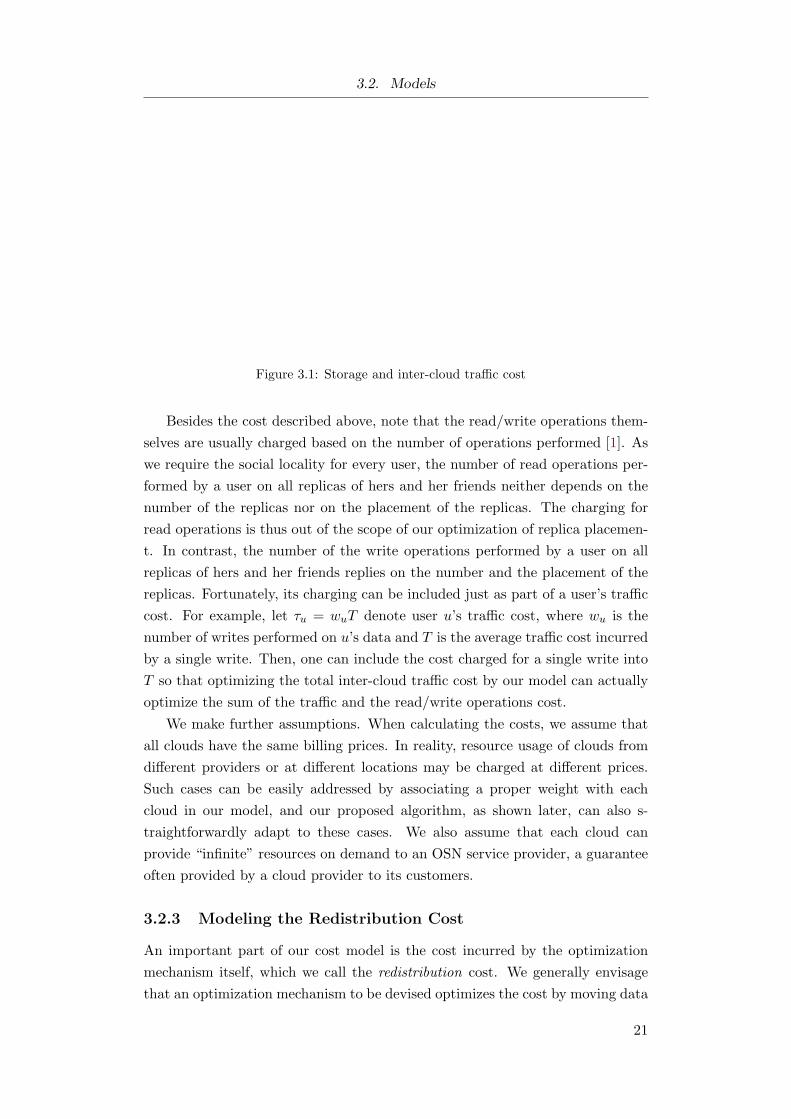
Fig. 3.1 is an example where 11 users are hosted by 3 clouds. Black circles

represent each user’s master replica, and red ones represent the slave replicas

of neighbors to ensure social locality. Solid lines are social relations and dotted

arrows are the synchronization traffic. Within each black circle, the value on the

top is the storage cost of a user, and the value at bottom is the traffic cost. For

this placement, we can find the total storage cost is 330 and the total inter-cloud

traffic cost is 50.

20

3.2. Models

(3, 1, 2) I K

J

(2, 1, 3)

(3, 1, 2)

A B

D

E G

F

H

(1, 3, 2)

(1, 2, 3) (3, 1, 2)

(1, 2, 3) (2, 1, 3)

(2, 3, 1)

(1, 2, 3) (3, 2, 1)

Cloud 1

23

10

C 11

9

36

2

20

7

I’

E’

C’

B’ 6

5

27

5 15

1

10

4 K’

Cloud 2

Cloud 3

C’’

25

2 32

10

11

3 E’’

Master replica

Slave replica

Social relation

Sorted clouds

Storage cost

Traffic cost

Inter-cloud traffic

Figure 3.1: Storage and inter-cloud traffic cost

Besides the cost described above, note that the read/write operations them-

selves are usually charged based on the number of operations performed [1]. As

we require the social locality for every user, the number of read operations per-

formed by a user on all replicas of hers and her friends neither depends on the

number of the replicas nor on the placement of the replicas. The charging for

read operations is thus out of the scope of our optimization of replica placemen-

t. In contrast, the number of the write operations performed by a user on all

replicas of hers and her friends replies on the number and the placement of the

replicas. Fortunately, its charging can be included just as part of a user’s traffic

cost. For example, let τu = wuT denote user u’s traffic cost, where wu is the

number of writes performed on u’s data and T is the average traffic cost incurred

by a single write. Then, one can include the cost charged for a single write into

T so that optimizing the total inter-cloud traffic cost by our model can actually

optimize the sum of the traffic and the read/write operations cost.

We make further assumptions. When calculating the costs, we assume that

all clouds have the same billing prices. In reality, resource usage of clouds from

different providers or at different locations may be charged at different prices.

Such cases can be easily addressed by associating a proper weight with each

cloud in our model, and our proposed algorithm, as shown later, can also s-

traightforwardly adapt to these cases. We also assume that each cloud can

provide “infinite” resources on demand to an OSN service provider, a guarantee

often provided by a cloud provider to its customers.

3.2.3 Modeling the Redistribution Cost

An important part of our cost model is the cost incurred by the optimization

mechanism itself, which we call the redistribution cost. We generally envisage

that an optimization mechanism to be devised optimizes the cost by moving data

21


across clouds to optimum locations, thus incurring such cost. The redistribution

cost is essentially the inter-cloud traffic cost, but in this chapter we use the

term inter-cloud traffic to specifically refer to the inter-cloud write traffic for

maintaining replica consistency, and treat the redistribution cost separately.

We expect that the optimization is executed at a per-billing-period granular-

ity (e.g., per-month) for the following reasons. First, this frequency is consistent

with the billing period, the usual charging unit for a continuously running and

long-term online service. The OSN provider should be enabled to decide whether

to optimize the cost for each billing period, according to her monetary budget

and expected profit, etc. Also, applying any cost optimization mechanism too

frequently may fail the optimization itself. At the time of writing this chapter,

the real-world price of inter-cloud traffic for transferring some data once is quite

similar to that of storing the same amount of data for an entire billing peri-

od [1, 6]. As a result, moving data too frequently can incur more redistribution

cost that can hardly be compensated by the saved storage and inter-cloud traffic

cost. Without loss of generality, we assume that the optimization mechanism is

applied only once at the beginning of each billing period, i.e., the redistribution

cost only occurs at the beginning of every billing period.

3.2.4 Approximating the Total Cost

Consider the social graph in a billing period. As it may vary within the pe-

riod, we denote the final steady snapshot of the social graph in this period as

G′ = (V ′, E′), and the initial snapshot of the social graph at the beginning of

this period as G = (V,E). Thus, the graph G experiences various changes—

collectively called ∆G—to become G′, where ∆G = (∆V,∆E), ∆V = V ′ − V ,

and ∆E = E′ − E.

Now consider the total cost incurred during a billing period. Denoting the

total cost, the storage plus the inter-cloud traffic cost, the maintenance cost, and

the redistribution cost during a period as Ψ, Φ(·), Ω(·), and Θ(·), respectively,

we have

Ψ = Φ(G) + Φ(∆G) + Ω(∆G) + Θ(G).

The storage cost in Φ(G) + Φ(∆G) is for storing users’ data replicas, including

the data replicas of existing users and of those who just join the service in this

period. The inter-cloud traffic cost in Φ(G)+Φ(∆G) is for propagating all users’

writes to maintain replica consistency. The redistribution cost Θ(G) is the cost

of moving data across clouds for optimization; it is only incurred at the beginning

of a period, following our previous assumption. There is also some underlying

cost Ω(∆G) for maintenance, described as follows.

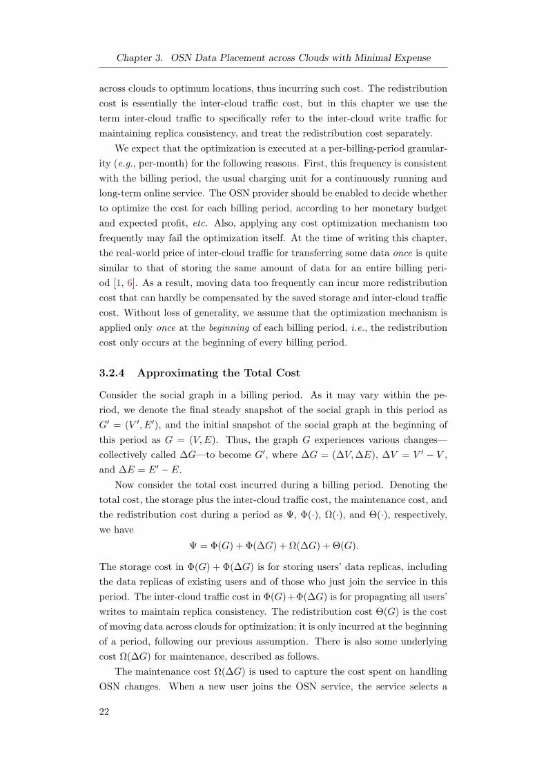
The maintenance cost Ω(∆G) is used to capture the cost spent on handling

OSN changes. When a new user joins the OSN service, the service selects a

22

3.2. Models

ti

Social

graph

Initial

distribution

Optimization

mechanism

1

2

3

1

3

2

1

2

3

2

1

3

1

3

2

1

2

3

Maintenance cost

Redistribution cost

Storage and inter-cloud traffic cost

Figure 3.2: Different types of costs

2

t0 t1 t2 t3

Social

graph

Initial

distribution

Optimization

mechanism

1

2

3

1

2

3

1

1

2

3

2

1

3

3

1 3

2

1

2

3

2

1

3

Figure 3.3: Cost over time

cloud and places this user’s data there. Some time later after this initial place-

ment and no later than the end of the current billing period, the OSN service

must maintain social locality for this user and her neighbors, including creating

new slave replicas on involved clouds as needed, causing the maintenance cost.

However, in reality, Ω(∆G), as well as Φ(∆G), become negligible as the size of

∆G (i.e., |∆V |) becomes much smaller than that of G (i.e., |V |) when the OS-

N user base reaches a certain scale. Existing research observes that real-world

OSNs usually have an S-shape growth [19, 33]. As the user population becomes

larger, the increment of the total number of users or social relations will decay

exponentially [46, 96]. Let us look at the monthly growth rate (i.e., |∆V |/|V |) in

some real examples. According to Facebook [4], after its user population reached

58 million by the end of 2007, it grew with an average monthly rate below 13%

through 2008 and 2009, a rate below 6% through 2010, and then a rate below

4% until the end of 2011 when it reached 845 million. For Twitter, its average

monthly growth rate was less than 8% in most months between March 2006 and

September 2009 [10]; similar rates were observed for YouTube and Flickr [63].

Therefore, we derive an approximated cost model as

Ψ ≈ Φ(G) + Θ(G)

which we will focus on throughout the rest of this chapter. Note that calculating

Ψ requires the storage cost and the traffic cost of each user in G. For any

cost optimization mechanism that runs at the beginning of a billing period, an

estimation is required to predict each user’s costs during this billing period.

Let’s for now deem that the costs can be estimated and known. We defer the

discussion on cost estimation to Section 3.5.1.

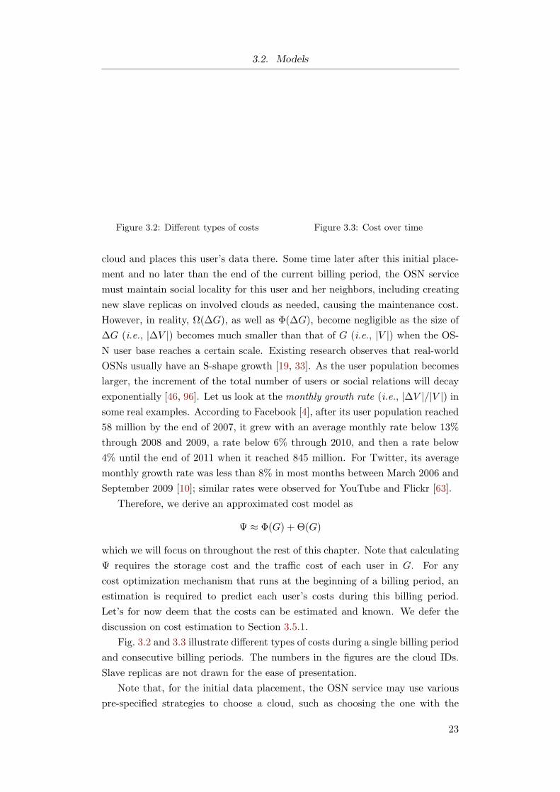
Fig. 3.2 and 3.3 illustrate different types of costs during a single billing period

and consecutive billing periods. The numbers in the figures are the cloud IDs.

Slave replicas are not drawn for the ease of presentation.

Note that, for the initial data placement, the OSN service may use various

pre-specified strategies to choose a cloud, such as choosing the one with the

23


lowest access latency for the user [80, 82]. At this time point the OSN cannot

determine an optimum cloud in terms of cost for a new user, as it knows neither

the user’s storage cost (except for a certain reserved storage such as storing a

profile with pre-filled fields) nor her traffic cost for the current billing period.

We assume that an OSN places a new user’s data on her most preferred cloud.

3.2.5 Modeling QoS and Data Availability

Sorting clouds: Among all clouds, one cloud can be better than another for a

particular user in terms of certain metric(s) (e.g., access latency, security risk).

For instance, concerning access latency, the best cloud to host the data requested

by a user is likely the geographically closest cloud to that user. Given N clouds

and |V | users, with cloud IDs 1, . . . , N (denoted as [N ] hereafter) and user

IDs 1, . . . , |V | (denoted as [|V |] hereafter), clouds can be sorted for user u as

~cu = (cu1, cu2, ..., cuN ), where cui ∈ [N ], ∀i ∈ [N ]. For any cloud cui, cuj , i < j,

we deem that cui is more preferred than cuj ; in other words, placing user u’s

data on the former provides better service quality to this user than the latter.

The clouds cu1, cu2, ..., cuj, ∀j ∈ [N ] are thus the j most preferred clouds of

user u, and the cloud cuj is the jth most preferred cloud of user u. This sorting

approach provides a unified QoS abstraction for every user while making the

underlying metric transparent to the rest of the QoS model.

Defining QoS: We define the QoS of the entire OSN service as a vector

~q = (~q[1], ~q[2], ..., ~q[N ]), with

~q[k] =1

|V |

|V |∑

u=1

k∑

j=1

fu(mu, j), ∀k ∈ [N ],

where mu denotes the ID of the cloud that hosts the master data replica of user

u, fu(i, j) is a binary function that equals to 1 if cloud i is user u’s jth most

preferred cloud but 0 otherwise. Therefore, ~q[k] is the ratio of users whose master

data are placed on any of their respective k most preferred clouds over the entire

user population. This CDF-style vector allows OSN providers to describe QoS

at a finer granularity.

Let us refer back to Fig. 3.1 as an example, where the vector associated with

each circle represents the sorted cloud IDs for the corresponding user. We see

that out of all the 11 users, 7 are hosted on their first most preferred cloud, 10

on either of their two most preferred clouds, and all users on any of their three

most preferred clouds. Thus, the QoS is ~q = ( 711 ,

1011 , 1).

Comparing QoS: There can be different data placements upon clouds.

Each may result in a different corresponding QoS vector. For two QoS vectors

~qa and ~qb representing two placements respectively, we deem that the former

placement provides QoS no better than the latter, i.e., ~qa ≤ ~qb, if every element

24

3.3. Problem

of the former vector is no larger than the corresponding element of the latter,

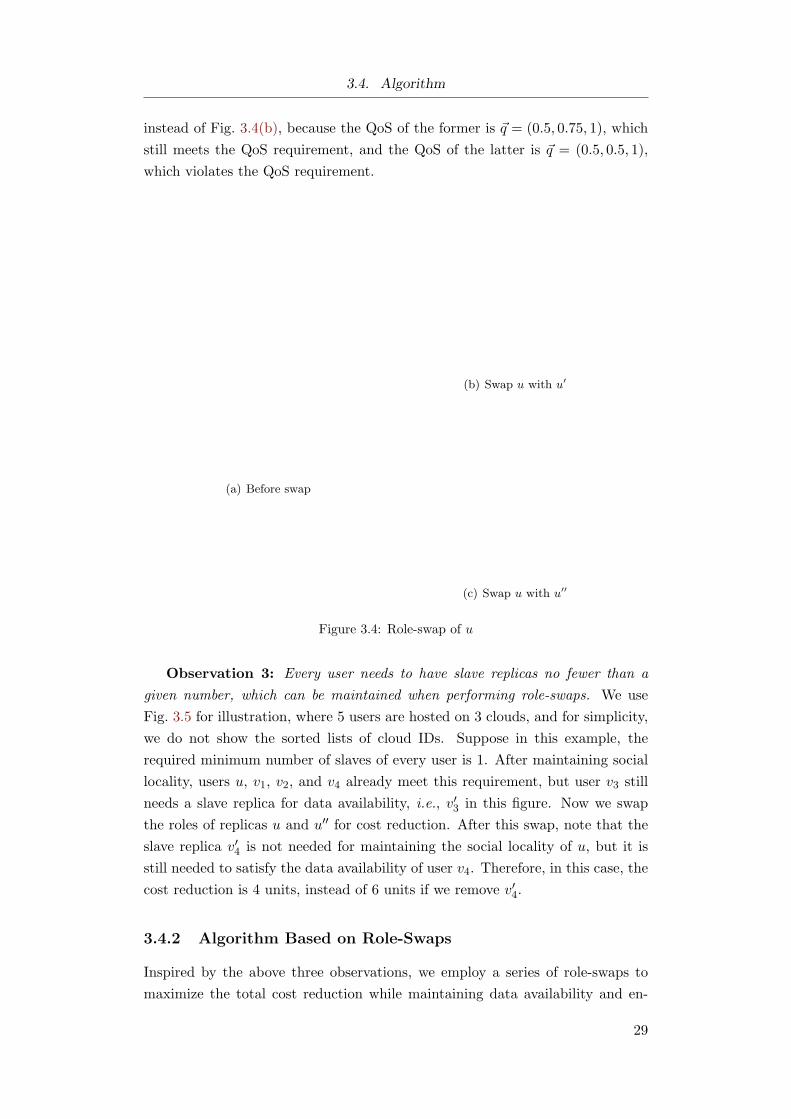
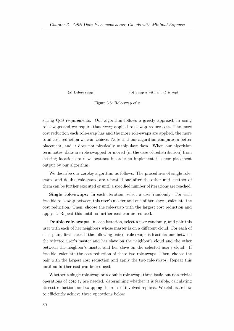
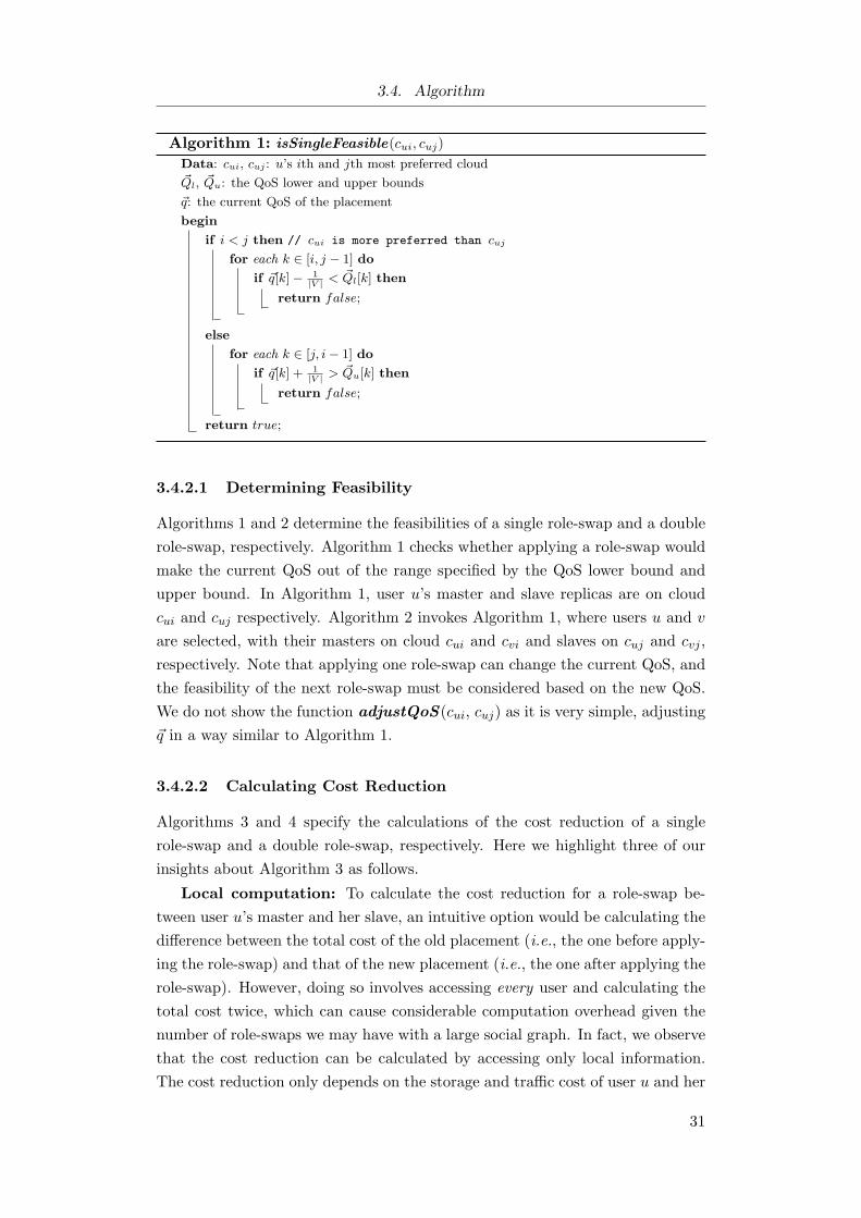
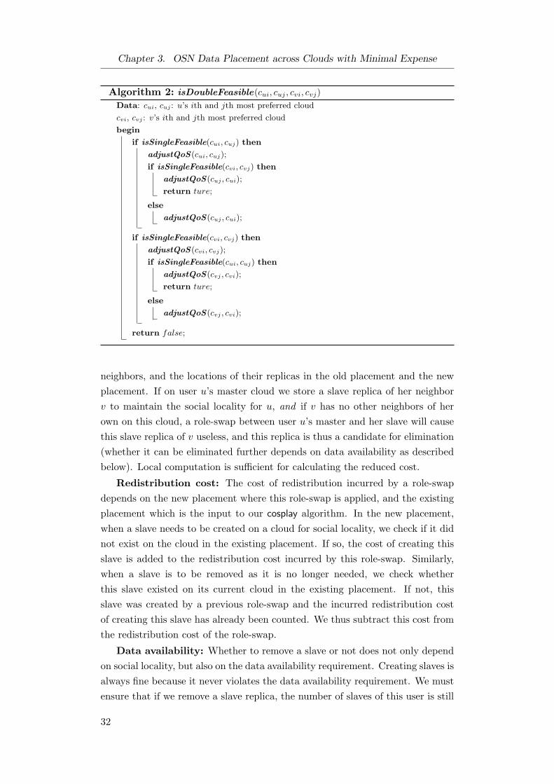
i.e., ~qa[k] ≤ ~qb[k], ∀k ∈ [N ].

QoS requirement: We model the QoS requirement as two vectors ~Ql and~Qu, ~Ql ≤ ~Qu that serve as a lower bound and an upper bound, respectively. In

order to meet the QoS requirement, a data placement must have a QoS ~q that

meets ~Ql ≤ ~q ≤ ~Qu. Specified by the OSN provider, ~Ql captures the worst QoS

that can be tolerated and ~Qu captures the best QoS that can be provided. Note

that we do not require ~Qu represent the placement of every user’s data on her

first most preferred cloud. ~Qu can be set as any valid QoS vector, subject to the

OSN provider’s customized policies and considerations.

As an example, let us see how ~Ql can express “80% of all users must access

data in no more than 200 ms.” In this case, clouds are sorted according to access

latency for every user. For any user u, we can calculate that only putting her

master data replica on any of her nu, nu ∈ [N ] most preferred clouds can grant

her the latency of no more than 200 ms. By denoting nmin = minnu|∀u ∈

[|V |], this requirement can thus be expressed by setting ~Ql[nmin] = 0.8. If

nmin 6= 1, then ~Ql[k], ∀k ∈ 1, . . . , nmin − 1 can be set as any value as long as

0 ≤ ~Ql[k1] ≤ ~Ql[k2] ≤ 0.8, 1 ≤ k1 < k2 < nmin. In fact, ~Ql can express any

fine-grained requirement such as “95% of users’ access must be satisfied within

500 ms, 80% be satisfied within 200 ms and 65% be satisfied within 90 ms.”

Data availability requirement: An OSN provider specifies the data avail-

ability requirement by indicating the minimum number of every user’s slave

replicas. We denote it using a number R, R ∈ 0, . . . , N − 1, where N is the

number of clouds. In order to meet the data availability requirement, each user

must maintain slave replicas no fewer than R. If the number of a user’s slave

replicas to maintain social locality is no smaller than R, the data availability

requirement for this user has already been met and this user does not have to

own more slaves; in contrast, besides the slaves to maintain social locality, if a

user does not have enough slaves to meet the data availability requirement, then

this user must have more slaves to ensure that the total number of her slaves is

equal to R.

3.3 Problem

3.3.1 Problem Formulation

With the models defined in Section 3.2, we are interested in the following prob-

lem: given an existing data placement upon N clouds of OSN G(V,E) with |V |

users, find out the optimal data placement with the minimal total cost—i.e., the

sum of the storage and inter-cloud traffic cost Φ(G) and the redistribution cost

Θ(G) for implementing this optimal placement from the existing placement—

25


while ensuring QoS and data availability meet pre-defined requirements.

We introduce the following notations in order to formulate the problem. mui

and sui are binary decision variables. The former equals to 1 if in the optimal

placement user u’s master replica is placed on cloud i, and 0 otherwise. The

latter equals to 1 if in the optimal placement u has a slave replica placed on cloud

i, and 0 otherwise. m′ui and s′ui are also binary, and are counterparts of mui and

sui respectively in the existing placement. µu is the storage cost for storing one

master or slave replica of user u. τu is the traffic cost for synchronizing one

slave replica of user u. β is the coefficient for converting the storage cost of a

replica to the redistribution cost of moving this replica across clouds. euv ∈ E if

user u and user v are neighbors. fu(i, j) is a binary function indicating whether

cloud i is user u’s jth most preferred cloud (as introduced in Section 3.2.5). The

QoS requirement is given by two vectors ~Ql and ~Qu, and the data availability

requirement is given by a number R. We formulate the problem as follows.

minimize

Φ(G) + Θ(G)

where

Φ(G) =

|V |∑

u=1

(µu

N∑

i=1

(mui + sui) + τu

N∑

i=1

sui)

Θ(G) =

|V |∑

u=1

(βµu

N∑

i=1

(max(mui + sui)− (m′ui + s′ui), 0))

subject to

N∑

i=1

mui = 1, ∀u ∈ [|V |] (3.1)

mui + sui ≤ 1, ∀u ∈ [|V |], ∀i ∈ [N ] (3.2)

mvj + svj = 1, j =N∑

i=1

(imui), if euv ∈ E, ∀u, v ∈ [|V |] (3.3)

N∑

i=1

sui ≥ R, ∀u ∈ [|V |] (3.4)

~Ql[k] ≤1

|V |

|V |∑

u=1

k∑

j=1

fu(

N∑

i=1

(i ·mui), j) ≤ ~Qu[k], ∀k ∈ [N ] (3.5)

Constraint (3.1) ensures that every user has a single master replica. Con-

straint (3.2) ensures that no master and slave replicas of the same user are

co-located on a common cloud. Constraint (3.3) ensures the social locality.

Constraint (3.4) ensures the data availability. Constraint (3.5) ensures that the

26

3.3. Problem

QoS of the data placement meets the QoS requirement. All constraints apply

to both the existing data placement and the optimal placement. Here we do

not write the existing case for the ease of presentation. Our cost optimization

problem is NP-hard.

3.3.2 Contrast with Existing Problems

To the best of our knowledge, existing problems that are most related to our

problem defined above are likely the MIN REPLICA [73] problem and the graph

partitioning [52] problem. Here we highlight why they fail to capture our scenario

in this chapter.

The MIN REPLICA problem minimizes the total number of replicas of user-

s’ data while maintaining social locality, load balance across partitions, and a

given redundancy. Compared with our problem, it falls short in the following as-

pects. First, it does not consider QoS. It balances the number of master replicas

across servers within a single cloud, while we aim to place masters across mul-

tiple clouds in order to ensure QoS meet a pre-defined requirement. Second, it

does not consider data redistribution, as it targets intra-cloud placement where

redistribution is free. In our case, the redistribution cost is inter -cloud and is an

important part of our objective. Third, it does not model the storage cost and

the traffic cost of each user. It minimizes the total number of replicas, while we

aim to minimize the total monetary cost that an OSN service provider has to

pay to the cloud provider.

The graph partitioning problem minimizes the total amount of communica-

tion volume or the total weights of edges across partitions while maintaining

load balance. Compared with our problem, it has no notion of social locality at

all, neither does it capture the QoS and the data availability requirements.

3.3.3 NP-Hardness Proof

We prove the NP-hardness of our cost optimization problem by restriction.

Specifically, we show that the MIN REPLICA problem, which has been proved

NP-hard [73], is contained by our problem as a special case. Firstly, let β = 0

and let µu = 0, τu = 1, ∀u ∈ [1,M ]. This makes the objective of our cost op-

timization problem the same as that of MIN REPLICA, both minimizing the

total number of slave replicas. Secondly, let the list of the sorted clouds of ev-

ery user be identical, i.e., fu(i, j) = fv(i, j), ∀u, v ∈ [1,M ], ∀i, j ∈ [1, N ], and

let ~Ql and ~Qu satisfy ~Ql[k] = ~Qu[k] =kN, ∀k ∈ [1, N ]. This makes Constraint

(3.5) of our problem equivalent to the load balance constraint of MIN REPLICA,

both maintaining an equal number of master replicas across partitions. Thirdly,

note that all other constraints of our problem are the same as their counterparts

of MIN REPLICA. Hence, MIN REPLICA is a case of our problem under the

27


above settings. Due to the NP-hardness of MIN REPLICA, our cost optimiza-

tion problem is NP-hard.

3.4 Algorithm

Our cost optimization problem is an Integer Programming (IP) problem [68].

The huge user population of real-world OSN services translates into a huge

number of decision variables, and the NP-hardness of our problem makes it

impossible to be efficiently solved by existing general-purpose IP solvers. We

thus seek practical heuristics. We propose cosplay, an optimization algorithm

that iteratively swaps the roles of master and slave replicas on different clouds

in order to adjust an existing placement towards the optimal placement.

3.4.1 Observations of Role-Swaps

Our algorithm is inspired by three observations below when swapping a master

replica and a slave replica of a user. In this what we call a role-swap process, the

master replica becomes a slave replica and the slave becomes the master. We

use Fig. 3.4 and Fig. 3.5 to illustrate our observations, where lines and circles

in these figures have the same meanings as in Fig. 3.1, and each user has 1 unit

of storage cost and 1 unit of traffic cost. Note that while symbols like u, v are

supposed to denote users throughout this chapter, we also use them to denote

the master replicas of the corresponding users in the figures here.

Observation 1: Role-swap can lead to possible cost reduction. Fig. 3.4 is

a simple example with 4 users hosted by 3 clouds. For user u, we may choose

to swap the roles of replica u with replica u′ (as in Fig. 3.4(b)), or swap the

roles of replica u with replica u′′ (as in Fig. 3.4(c)), while maintaining the social

locality. Before the swap as in Fig. 3.4(a), there are 10 units of replica storage

and 6 units of inter-cloud traffic. After the swap, as either in Fig. 3.4(b) or in

Fig. 3.4(c), there are 9 units of replica storage and 5 units of inter-cloud traffic.

We thus save 1 unit of replica storage and 1 unit of inter-cloud traffic by paying

1 unit of redistribution cost (caused by copying the replica v3 to create a new

replica v′3 in Fig. 3.4(b), or v′′3 in Fig. 3.4(c)). Overall, we can achieve 1 unit of

cost reduction.

Observation 2: Because of the QoS requirement, not every role-swap is

feasible. When multiple role-swaps for a user are available, we must choose the

one(s) meeting QoS requirements. The two different role-swap choices taken in

Fig. 3.4(b) and in Fig. 3.4(c) result in the same amount of cost reduction. Let us

suppose every cloud has an ID and every user has a sorted list of preferred clouds

as shown in the figure. Before swap, ~q = (0.75, 0.75, 1). If the QoS requirement is

given by ~Qu = (1, 1, 1) and ~Ql = (0.5, 0.75, 1), then we should choose Fig. 3.4(c)

28

3.4. Algorithm

instead of Fig. 3.4(b), because the QoS of the former is ~q = (0.5, 0.75, 1), which

still meets the QoS requirement, and the QoS of the latter is ~q = (0.5, 0.5, 1),

which violates the QoS requirement.

Cloud 1 Cloud 2

Cloud 3

ଷݒ

ଶݒ

ଵݒ

ଵԢݒ

ԢԢݑ ଵԢԢݒ

ݑ ଶԢԢݒ Ԣݑ

ଶԢݒ(1,3,2)

(3,2,1)

(3,1,2)

(2,1,3)

(a) Before swap

ଷݒ

ଶݒ

ଵݒ

Ԣݑ

ԢԢݑ ଵԢԢݒ ݑ ଶԢԢݒ

ଷԢݒ(1,3,2)

(3,2,1)

(3,1,2)

(2,1,3)

Cloud 1 Cloud 2

Cloud 3

(b) Swap u with u′

ଷݒ

ଶݒ

ଵݒ

ݑ ଵԢԢݒ

ԢԢݑ ଶԢԢݒ ԢݑCloud 1 Cloud 2

Cloud 3

ଷԢԢ (1,3,2)ݒ

(3,2,1)

(3,1,2)

(2,1,3)

(c) Swap u with u′′

Figure 3.4: Role-swap of u

Observation 3: Every user needs to have slave replicas no fewer than a

given number, which can be maintained when performing role-swaps. We use

Fig. 3.5 for illustration, where 5 users are hosted on 3 clouds, and for simplicity,

we do not show the sorted lists of cloud IDs. Suppose in this example, the

required minimum number of slaves of every user is 1. After maintaining social

locality, users u, v1, v2, and v4 already meet this requirement, but user v3 still

needs a slave replica for data availability, i.e., v′3 in this figure. Now we swap

the roles of replicas u and u′′ for cost reduction. After this swap, note that the

slave replica v′4 is not needed for maintaining the social locality of u, but it is

still needed to satisfy the data availability of user v4. Therefore, in this case, the

cost reduction is 4 units, instead of 6 units if we remove v′4.

3.4.2 Algorithm Based on Role-Swaps

Inspired by the above three observations, we employ a series of role-swaps to

maximize the total cost reduction while maintaining data availability and en-

29


ଷݒ

ଶݒ

ଵݒ

ଵԢݒ

ԢԢݑ ଵԢԢݒ ݑ ଶԢԢݒ Ԣݑ

ଶԢݒ

ଷԢݒ ସݒ ସԢݒ

(a) Before swap

ଷݒ

ଶݒ

ଵݒ

ݑ ଵԢԢݒ

ସԢݒ ԢԢݑ ଶԢԢݒ Ԣݑ ଷԢݒ ସݒ

(b) Swap u with u′′: v′4 is kept

Figure 3.5: Role-swap of u

suring QoS requirements. Our algorithm follows a greedy approach in using

role-swaps and we require that every applied role-swap reduce cost. The more

cost reduction each role-swap has and the more role-swaps are applied, the more

total cost reduction we can achieve. Note that our algorithm computes a better

placement, and it does not physically manipulate data. When our algorithm

terminates, data are role-swapped or moved (in the case of redistribution) from

existing locations to new locations in order to implement the new placement

output by our algorithm.

We describe our cosplay algorithm as follows. The procedures of single role-

swaps and double role-swaps are repeated one after the other until neither of

them can be further executed or until a specified number of iterations are reached.

Single role-swaps: In each iteration, select a user randomly. For each

feasible role-swap between this user’s master and one of her slaves, calculate the

cost reduction. Then, choose the role-swap with the largest cost reduction and

apply it. Repeat this until no further cost can be reduced.

Double role-swaps: In each iteration, select a user randomly, and pair this

user with each of her neighbors whose master is on a different cloud. For each of

such pairs, first check if the following pair of role-swaps is feasible: one between

the selected user’s master and her slave on the neighbor’s cloud and the other

between the neighbor’s master and her slave on the selected user’s cloud. If

feasible, calculate the cost reduction of these two role-swaps. Then, choose the

pair with the largest cost reduction and apply the two role-swaps. Repeat this

until no further cost can be reduced.

Whether a single role-swap or a double role-swap, three basic but non-trivial

operations of cosplay are needed: determining whether it is feasible, calculating

its cost reduction, and swapping the roles of involved replicas. We elaborate how

to efficiently achieve these operations below.

30

3.4. Algorithm

Algorithm 1: isSingleFeasible(cui, cuj)

Data: cui, cuj : u’s ith and jth most preferred cloud~Ql, ~Qu: the QoS lower and upper bounds

~q: the current QoS of the placement

begin

if i < j then // cui is more preferred than cuj

for each k ∈ [i, j − 1] do

if ~q[k]− 1

|V |< ~Ql[k] then

return false;

else

for each k ∈ [j, i− 1] do

if ~q[k] + 1

|V |> ~Qu[k] then

return false;

return true;

3.4.2.1 Determining Feasibility

Algorithms 1 and 2 determine the feasibilities of a single role-swap and a double

role-swap, respectively. Algorithm 1 checks whether applying a role-swap would

make the current QoS out of the range specified by the QoS lower bound and

upper bound. In Algorithm 1, user u’s master and slave replicas are on cloud

cui and cuj respectively. Algorithm 2 invokes Algorithm 1, where users u and v

are selected, with their masters on cloud cui and cvi and slaves on cuj and cvj ,

respectively. Note that applying one role-swap can change the current QoS, and

the feasibility of the next role-swap must be considered based on the new QoS.

We do not show the function adjustQoS(cui, cuj) as it is very simple, adjusting

~q in a way similar to Algorithm 1.

3.4.2.2 Calculating Cost Reduction

Algorithms 3 and 4 specify the calculations of the cost reduction of a single

role-swap and a double role-swap, respectively. Here we highlight three of our

insights about Algorithm 3 as follows.

Local computation: To calculate the cost reduction for a role-swap be-

tween user u’s master and her slave, an intuitive option would be calculating the

difference between the total cost of the old placement (i.e., the one before apply-

ing the role-swap) and that of the new placement (i.e., the one after applying the

role-swap). However, doing so involves accessing every user and calculating the

total cost twice, which can cause considerable computation overhead given the

number of role-swaps we may have with a large social graph. In fact, we observe

that the cost reduction can be calculated by accessing only local information.

The cost reduction only depends on the storage and traffic cost of user u and her

31


Algorithm 2: isDoubleFeasible(cui, cuj , cvi, cvj)

Data: cui, cuj : u’s ith and jth most preferred cloud

cvi, cvj : v’s ith and jth most preferred cloud

begin

if isSingleFeasible(cui, cuj) then

adjustQoS(cui, cuj);

if isSingleFeasible(cvi, cvj) then

adjustQoS(cuj , cui);

return ture;

else

adjustQoS(cuj , cui);

if isSingleFeasible(cvi, cvj) then

adjustQoS(cvi, cvj);

if isSingleFeasible(cui, cuj) then

adjustQoS(cvj , cvi);

return ture;

else

adjustQoS(cvj , cvi);

return false;

neighbors, and the locations of their replicas in the old placement and the new

placement. If on user u’s master cloud we store a slave replica of her neighbor

v to maintain the social locality for u, and if v has no other neighbors of her

own on this cloud, a role-swap between user u’s master and her slave will cause

this slave replica of v useless, and this replica is thus a candidate for elimination

(whether it can be eliminated further depends on data availability as described

below). Local computation is sufficient for calculating the reduced cost.

Redistribution cost: The cost of redistribution incurred by a role-swap

depends on the new placement where this role-swap is applied, and the existing

placement which is the input to our cosplay algorithm. In the new placement,

when a slave needs to be created on a cloud for social locality, we check if it did

not exist on the cloud in the existing placement. If so, the cost of creating this

slave is added to the redistribution cost incurred by this role-swap. Similarly,

when a slave is to be removed as it is no longer needed, we check whether

this slave existed on its current cloud in the existing placement. If not, this

slave was created by a previous role-swap and the incurred redistribution cost

of creating this slave has already been counted. We thus subtract this cost from

the redistribution cost of the role-swap.

Data availability: Whether to remove a slave or not does not only depend

on social locality, but also on the data availability requirement. Creating slaves is

always fine because it never violates the data availability requirement. We must

ensure that if we remove a slave replica, the number of slaves of this user is still

32

3.4. Algorithm

Algorithm 3: calcCostReducSingle(mu, su)

Data: mu: the cloud hosting u’s master replica

su: the cloud hosting u’s slave replica

µu, τu: u’s storage cost and traffic cost

Pe: the existing placement of all users’ replicas

∆: the cost that can be reduced

δu: the number of u’s slaves that can be reduced

ρ: the number of slaves that incur the redistribution cost

Rmv mu: boolean: true if removing u’s replica on mu, false if not

Rmv su: boolean: true if removing u’s replica on su, false if not

begin

∆⇐ 0, δu ⇐ 0, δv ⇐ 0, ρ⇐ 0;

Rmv mu ⇐ true, Rmv su ⇐ true;

/* calculate the reduced cost incurred by replicas of u’s neighbors */

for each v ∈ u’s neighbors do

δv ⇐ 0, ρ⇐ 0;

if mv 6= mu then

if u is v’s only neighbor on mu then

δv ⇐ δv + 1;

if v has no replica on mu in Pe then

ρ⇐ ρ− 1;

if mv = su then

Rmv su ⇐ false;

if mv 6= su then

if v has no slave replica on su then

δv ⇐ δv − 1;

if v has no replica on su in Pe then

ρ⇐ ρ+ 1;

if mv = mu then

Rmv mu ⇐ false;

if ¬ (v has R slave replicas and δv > 0) then

∆⇐ ∆+ (µv + τv)δv − βµvρ;

/* calculate the reduced cost incurred by replicas of u’s own */

ρ⇐ 0;

if Rmv su = true then

δu ⇐ δu − 1;

if u has no replica on su in Pe then

ρ⇐ ρ+ 1;

if Rmv mu = true then

δu ⇐ δu + 1;

if u has no replica on mu in Pe then

ρ⇐ ρ− 1;

if ¬ (u has R slave replicas and δu > 0) then

∆⇐ ∆+ (µu + τu)δu − βµuρ;

return ∆;

33


Algorithm 4: calcCostReducDouble(mu, su,mv, sv)

begin

∆Ψ1 ⇐ calcCostReducSingle(mu, su);

swapRole(mu, su);

∆Ψ2 ⇐ calcCostReducSingle(mv, sv);

swapRole(su,mu);

return ∆Ψ1 +∆Ψ2;

Algorithm 5: swapRole(mu, su)

Data: mu: the cloud hosting u’s master replica

su: the cloud hosting u’s slave replica

δu: the number of u’s slaves that can be reduced

Rmv mu: boolean: true if removing u’s replica on mu, false if not

begin

δu ⇐ 0, δv ⇐ 0, Rmv mu ⇐ true;


δv ⇐ 0, ρ⇐ 0;

if mv 6= mu then


δv ⇐ δv + 1;

if mv 6= su then


δv ⇐ δv − 1;

if mv = mu then

Rmv mu ⇐ false;

if ¬ (v has R slave replicas and δv > 0) then

if mv 6= mu then


Remove v’s slave at mu;

if mv 6= su then


Create v’s slave at su;

// Do the role-swap

if Rmv mu = true then

δu ⇐ δu + 1;

u’s master at mu becomes a slave;

u’s slave at su becomes the master;

if ¬ (u has R slave replicas and δu > 0) then

if u has a slave replica on mu and Rmv mu = true then

Remove u’s slave at mu;

34

3.5. Evaluations

no fewer than the pre-specified number, thus maintaining the data availability

for this user. If we cannot remove a slave due to data availability, this user should

not be considered when calculating cost reduction of a role-swap that involves

this user, and the slave is also not touched when performing the role-swap.

3.4.2.3 Swapping Roles of Replicas

Algorithm 5 describes the operation of swapping the roles of a user u’s master

on cloud mu and her slave on cloud su. Swapping the roles does not simply

involve u’s replicas alone; instead, it may also involve removing or creating her

neighbors’s slave replicas due to social locality and data availability. The flow of

this algorithm shares some similarities with that of Algorithm 1, as calculating

the cost reduction of a role-swap before it is performed is actually simulating

how the cost would be affected if the role-swap was performed.

3.5 Evaluations

We carry out extensive evaluations by placing real-world Twitter data over 10

clouds all across the US. We demonstrate significant one-time and accumulated

cost reductions compared to existing approaches, while always ensuring QoS

and data availability requirements. By varying the experimental settings, we

also investigate the complex trade-off among cost, QoS, and data availability.

3.5.1 Data Preparation

Collecting data: We crawled Twitter during March and April 2010 in a

breadth-first manner, consistent with previous OSN crawls [64, 85]. We col-

lected 3,117,553 users with 23,883,149 social relations. For each user, we have

her profile, tweets, and the list of followers. Among all the users, 1,157,425 users

provide location information in their profiles.

Sorting clouds for each user: Due to the lack of publicly available dataset

on latencies between OSN users and OSN sites, we cannot sort clouds for users

in terms of latency. However, the geographic distance is widely used as an

important QoS metric in previous work [29, 40]. With our Twitter dataset, we

thus sort clouds for each user in terms of the real-world geographic distance

between a user and the clouds.

We focus on users who are geographically located in the US. With the help

of the database of US Board on Geographic Names [8] and Google Maps, we

convert users’ text locations to geo-coordinates (i.e., [latitude, longitude]). Out

of all these users, we extract the largest connected component of 321,505 users

with 3,437,409 social relations as the input to our evaluations. We then select 10

cities all across the US as cloud locations: Seattle (WA), Palo Alto (CA), Orem

35


Figure 3.6: User locations

10 20 30 400

20%

40%

60%

80%

100%

120%

140%

160%

Month

10 20 30 400

50%

100%

150%

200%

250%

300%

350%

400%

Social relations growth rate

User population growth rate

Figure 3.7: Monthly growth rate

(UT), Chicago (IL), San Antonio (TX), Lansing (MI), Alexandria (LA), Atlanta

(GA), Ashburn (VA), and New York (NY). All these locations have real-world

cloud data centers [3]. Afterwards, we sort all clouds for each user in terms of

the respective geographic distance between a user and the clouds. Fig. 3.6 plots

the locations of all the 321,505 users.

Extracting monthly OSN snapshots: To evaluate cosplay for OSN with

dynamics, we extract monthly graph snapshots out of our largest connected com-

ponent. Under the assumption that each user publishes her first tweet and forms

her social relations immediately after she joins the service, and with the time

stamp of each tweet and the follower list of each user, we find that the earliest

user in our largest connected component joined Twitter in March 2006 and the

latest user joined Twitter in February 2010. We thus can extract 48 monthly

social graphs. Fig. 3.7 shows the monthly growth rates of our 48 graphs. The

user base growing at about 15% since the 16th month is a good approximation

of the real-world OSN growth, as discussed in Section 3.2.

Obtaining monthly costs for each user: We calculate costs by multiply-

ing the unit price with the data size, and use such calculated costs of each user

for each of the 48 months as the ground truth. We use $0.125/GB/month for

storage cost and $0.12/GB for inter-cloud traffic cost [6]. With each tweet and

its time stamp, we can easily find how much data a user publishes in a given

month (i.e., the traffic size of that month), and how much data this user has

accumulated by the end of a given month (i.e., the storage size of that month).

In real world when executing cosplay in consecutive billing periods, it needs an

estimate of each user’s costs for a period at the beginning of the period. Existing

research tells that users’ online activities are bursty and the inter-activity time

is heavy-tailed [21, 84], making the estimation of future activities difficult, not

to mention the estimation of the data size which is of our interest. However, our

goal here is not pursuing the estimation accuracy, but implying the trend of the

size of a user’s produced data so that we can make a right decision of role-swap.

We exploit the Exponentially Weighted Moving Average, a common approach for

36

3.5. Evaluations

similar purposes, to estimate the number of activities in a future time period

with the smoothing factor α = 0.9 to capture the burstiness of user activities.

By multiplying it with the average data size of all previous activities, we obtain

the estimation of the data size in a future time period. As a result, we obtain

48 monthly graphs with the estimated costs of each user for each month.

3.5.2 Experimental Settings

We run two groups of evaluations. In the first group, with our largest February

2010 social graph as input, we compare the costs and the QoS’ of the data

placements produced by the greedy method, the random method, SPAR, METIS

and cosplay, respectively. We also investigate how the costs are influenced by

the data availability requirement and by the QoS requirement. We ensure social

locality for all approaches for fair comparison. The greedy method places every

user’s master on her first most preferred cloud. The random method assigns a

user’s master to a cloud randomly. For SPAR, we implement it ourselves, and

we treat each social relation between two users as an edge creation event and

create a random permutation of all events to produce the edge creation trace

as input, following the method suggested in [73]. For METIS, there is an open-

source implementation from its authors. We use its option of minimizing the

inter-partition communication. We use each user’s storage cost plus her traffic

cost as the vertex size (in METIS’ terminology) to create its input. For cosplay,

we use the greedy method to produce an existing placement.

We vary the number of most preferred clouds that users use to place masters,

and we also vary the QoS and the data availability requirements. We have 10

clouds sorted for every user. Besides the 10-clouds case, we also compare the

cases when each user uses her 2, 4, 6, and 8 most preferred clouds for master

placement, respectively. We vary the QoS requirement by varying the lower

bound while keeping the upper bound fixed at ~Qu = (1). Note that, when there

are 10 clouds a QoS vector should have 10 elements, but we omit the consecutive

1’s at the end of a QoS vector for the ease of presentation. ~Qu = (1) corresponds

to the greedy placement and is the best QoS that can be provided. We vary ~Ql

by the following rule. Given the value of the first element (hereafter we call it the

“first value” for brevity) of the ~Ql vector and given the number of most preferred

clouds that users use, we set the values of all other elements of ~Ql by building a

linear growth from its first value to 1. For example, if the first value of ~Ql is 0.5

and users use 2 most preferred clouds, then ~Ql = (0.5, 1). With the same first

value, if users use 6 most preferred clouds, then ~Ql = (0.5, 0.6, 0.7, 0.8, 0.9, 1).

We vary the data availability requirement by iterating R from 0 to 9. We set

β = 1, reflecting the fact that the cost of moving some data across clouds once

is similar to that of storing the same data in the cloud for one month.

37


In the second group of evaluations, with the inputs of our 48 monthly OSN

snapshots with real-world costs and the other 48 monthly snapshots with esti-

mated costs, we focus on the continuous cost reduction that can be achieved by

cosplay, compared with the greedy method. For each month, we run greedy on

the former, representing the real-world common practice of placing user’s data

on the closest cloud for lowest access latency. We run cosplay on the former to

show the “ideal” cost reduction, assuming we know the exact costs of each user

for each month at the beginning of every month. We also run cosplay on the

latter, where replica locations are adjusted according to the estimated costs of

each user, to show the effectiveness of our estimation approach. Note that cos-

play runs only once at the beginning of every month. When new users join the

system during a month, each user is still placed by the greedy method. When

only using greedy, the total cost for each month is the sum of the storage and the

inter-cloud traffic cost, plus the maintenance cost. When running cosplay, the

total cost for each month additionally includes the redistribution cost. We use

the same ~Qu and β settings as in our first group of evaluations and only consider

the case where every user uses all 10 most preferred clouds. We set R = 0 and

the first value of ~Ql to be 0.5.

In the figures, the cost of every placement is normalized as the quotient of the

placement divided by the standard cost, where the standard cost is the cost of

the greedy placement with R = 0. The storage cost is normalized by the standard

storage cost, the inter-cloud traffic cost and the redistribution cost is normalized

by the standard inter-cloud traffic cost, and the total cost is normalized by the

standard total cost.

3.5.3 Results on One-time Cost Reduction

We note that, throughout Fig. 3.8 to 3.11 and in Fig. 3.14 and 3.15, the first

value of ~Ql is always set as 0.5, and we vary ~Ql in Fig. 3.12 and 3.13.

Fig. 3.8 compares the costs of the placements produced by different methods

over all the 10 clouds with R = 0. For all methods except cosplay, the total cost

is the sum of its storage and inter-cloud traffic cost. For cosplay, the total cost

additionally includes the redistribution cost. The greedy placement has moderate

cost compared with random. Users who are geographically close to one another

tend to have similar sorted lists of clouds. Thus, greedy can assign local users to

the same nearby cloud and random tends to straddle local social relations across

clouds. SPAR has less cost than greedy and random but more than METIS,

indicating that minimizing the number of replicas cannot necessarily minimize

the cost. Cosplay outperforms all others with total cost reductions of 59%, 66%,

50% and 44%, compared to greedy, random, SPAR and METIS, respectively.

Fig. 3.9 depicts the total cost of each method over 10 clouds as R, the mini-

38

3.5. Evaluations

Storage Traffic Total0

0.4

0.8

1.2

1.6

No

rmalized

Co

st

greedy

random

SPAR

METIS

Cosplay

Figure 3.8: Cost comparison (I)

0 1 2 3 4 5 6 7 8 90

0.4

0.8

1.2

1.6

Minimum # of Slaves (R)

No

rma

lize

d T

ota

l C

os

t

greedy

random

SPAR

METIS

Cosplay

Figure 3.9: Cost comparison (II)

StorageTraffic Redis Total0

0.2

0.4

0.6

0.8

1.0

No

rmalized

Co

st

2 clouds

4 clouds

6 clouds

8 clouds

10 clouds

Figure 3.10: Cost of cosplay (I)

0 1 2 3 4 5 6 7 8 90

0.4

0.8

1.2

1.6


No

rma

lize

d T

ota

l C

os

t

2 clouds

4 clouds

6 clouds

8 clouds

10 clouds

Figure 3.11: Cost of cosplay (II)

mum number of slave replicas required for every user to ensure data availability,

varies. When R is small, cosplay achieves more cost reduction via role-swaps

and eliminates those slaves that are no longer needed for social locality. When it

becomes larger, cosplay’s advantages are decreasing, as it cannot eliminate some

slaves as they are needed for data availability even if they are not needed for

social locality. The room for optimization also becomes less. All methods turn

to full replication when R = 9.

Fig. 3.10 dissects the costs of the placements produced by cosplay on users’

2, 4, 6, 8, and 10 most preferred clouds in the case of R = 0. As the number of

involved clouds grows, the storage cost, the inter-cloud traffic cost and the total

cost drops, as more optimization can be done if more clouds are available for

each user. However, the redistribution cost also declines, indicating we pay less

overhead to save more costs. The reason is, as the total number of feasible role-

swaps grows, the number of users with negative redistribution cost also increases,

dragging down the total redistribution cost as more role-swaps place masters on

clouds where users do not have any replica in the existing placement.

Fig. 3.11 demonstrates the total cost of each cosplay placement as R increases.

No matter how R changes, we observe that when users consider placing their

masters on their most preferred clouds of more than 4, the advantages of cosplay

39


0.1 0.2 0.3 0.4 0.5 0.6 0.7 0.8 0.90

0.2

0.4

0.6

0.8

1.0

QoS Lower Bound First Value

No

rma

lize

d T

ota

l C

os

t

2 clouds

4 clouds

6 clouds

8 clouds

10 clouds

Figure 3.12: Cost of cosplay (III)

0.1 0.2 0.3 0.4 0.5 0.6 0.7 0.8 0.90

0.4

0.8

1.2

1.6


No

rma

lize

d T

ota

l C

os

t

10 clouds, R=2

10 clouds, R=4

10 clouds, R=6

10 clouds, R=8

Figure 3.13: Cost of cosplay (IV)

1 2 3 4 5 6 7 8 9 100

0.2

0.4

0.6

0.8

1.0

Most Preferred Cloud

Pro

po

rtio

n o

f U

se

rs

greedy

random

SPAR upper

SPAR lower

METIS upper

METIS lower

Cosplay

Required upper

Required lower

Figure 3.14: QoS comparison

0 1 2 3 4 5 6 7 8 90

1

2

3

4

5


# o

f S

laves f

or

Lo

cality

greedy

random

SPAR

METIS

Cosplay

Figure 3.15: Slave numbers

are not obviously influenced by the number of most preferred clouds. In contrast,

when every user only considers using her 2 most preferred clouds to host her

master, cosplay achieves much less cost reduction. This phenomenon implies that

2 most preferred clouds of each user do not seem to cover the social relations

among users, while 4 most preferred clouds of each user can have clouds of friends

overlapped and masters of friends co-located, and thus fewer slaves are needed

for social locality and the total cost can be much less than the 2-clouds case.

However, this advantage is gradually compensated as the minimum number of

slaves required by every user increases.

Fig. 3.12 shows the total costs cosplay achieves when the QoS requirement

varies with R = 0. As the first value of ~Ql increases, the number of users that are

allowed to be role-swapped decreases and thus less room is left for optimization.

When the first value is small, it does not affect the amount of cost that can be

saved. Although more users are allowed to be role-swapped, the number of role-

swaps that can lead to actual cost reduction is limited—allowing more users to be

role-swapped does not necessarily indicate more cost reduction. When the first

value becomes large enough, operating on fewer most preferred clouds achieves

more cost reduction, which aligns with our intuition that placing together a small

number of users instead of straddling them across clouds could save the cost. As

40

3.5. Evaluations

cosplay operates on a larger number of most preferred clouds, it is easier for

the cost reduction to be affected by the first value as this value grows. This is

natural as more clouds available means more role-swaps can be done to save cost.

Hence, it is easier to be affected when the number of permitted users decreases.

Fig. 3.13 provides the total costs cosplay achieves as both the QoS require-

ment and R vary when operating on all the 10 most preferred clouds. The case

with a larger R tends to be less affected by ~Ql than the case with a smaller R.

This is because when R is larger, the room for optimization becomes small due

to that the number of role-swaps that leads to cost reduction becomes small.

It can be small enough that even when R = 8 the QoS requirement does not

have any effect on the cost. With any given QoS requirement, a larger R always

comes with a lower cost reduction, consistent with Fig. 3.11.

Fig. 3.14 visualizes the QoS vectors of the placements produced by all the

methods over the 10 clouds. No doubt that greedy has the best QoS. Random

has the linear QoS as expected. SPAR or METIS partitions a graph into a given

number of partitions. With 10 clouds, there exist 10! = 3,628,800 different ways

of placing the 10 partitions upon the 10 clouds. Each placement has its own

QoS. Out of all 10! QoS vectors, we obtain the largest value and the smallest

value for each of the 10 dimensions of the QoS vector. We can therefore draw

the upper and lower QoS bounds for SPAR and METIS, respectively. SPAR

and METIS are only able to produce QoS similar to random, while cosplay can

always keep the QoS within any pre-defined upper and lower bounds.

Fig. 3.15 investigates how many more slaves we need to ensure the social

locality for every user, except the minimum number of slaves that are maintained

for data availability (some of them may also serve social locality). This figure

draws the average number of additional slaves needed for social locality in the

placements produced by different methods. We see that, while meeting the data

availability requirement, cosplay always needs the fewest number of additional

slaves for social locality of all users. Cosplay not only minimizes the cost, it also

reduces the number of replicas. What is interesting is that, SPAR, an algorithm

of minimizing the replica number, is beat by METIS. This is because SPAR

runs as a procedure of responding to a series of edge creation events and only

guarantees the minimal number of replicas of involved users in a local sense,

while METIS takes the whole social graph as input and thus achieves better

results in a global sense.

3.5.4 Results on Continuous Cost Reduction

We note that, as stated in Section 3.5.1, we mainly focus on the time periods

after the 16th month. The two peaks of user population growth in the 26th and

37th month are also reflected in our results.

41


10 20 30 400

5%

10%

15%

20%

25%

30%

35%

Month

Ma

inte

na

nc

e C

os

t o

ve

r T

ota

l C

os

t

greedy

Cosplay 2 clouds

Cosplay 4 clouds

Cosplay 6 clouds

Cosplay 8 clouds

Cosplay 10 clouds

Figure 3.16: Maintenance cost

10 20 30 400

1%

2%

Month

Re

dis

trib

uti

on

ov

er

To

tal

Co

st

Cosplay 2 clouds

Cosplay 4 clouds

Cosplay 6 clouds

Cosplay 8 clouds

Cosplay 10 clouds

Figure 3.17: Redistribution cost

10 20 30 400

10%

20%

20%

40%

Month

To

tal C

ost

Red

ucti

on

by C

osp

lay

One−month

Cumulative

One−month (estimation)

Cumulative (estimation)

Figure 3.18: 2 clouds

10 20 30 400

10%

20%

30%

40%

50%

Month

To

tal C

ost

Red

ucti

on

by C

osp

lay

One−month

Cumulative




Fig. 3.16 and 3.17 report the ratios of the maintenance cost and the redis-

tribution cost over the total cost in each month, respectively. Fig. 3.16 verifies

our cost model as the maintenance cost of greedy occupies less than 5% of the

total cost, which is the reason why we can neglect the maintenance cost incurred

by newly-joined users in our approximated cost model. Cosplay significantly re-

duces the total cost for each month, causing the maintenance cost to occupy

larger proportions out of the total cost. Fig. 3.17 shows that the redistribution

cost always keeps below 2% of the total cost of a month.

From Fig. 3.18 to Fig. 3.22, we find the one-time cost reduction for each

month and the cumulative cost reduction until each month, compared with

greedy. We make several observations. Firstly, our estimation approach per-

forms effectively. The one-month and the cumulative cost reductions achieved

by running cosplay on estimated costs do not deviate too much from, and al-

most overlap with reductions achieved by running cosplay on real-world costs.

Secondly, the cost reduction climbs up as time elapses, and increases as more

clouds are involved for each user. In the 10-clouds case, the accumulative total

cost reduction goes towards more than 40%. Thirdly, the cost reduction can

be deteriorated by large monthly growth rates, as in the months where local

peaks occur. However, as discussed previously, the real-world monthly growth

42

3.5. Evaluations

10 20 30 400

10%

20%

30%

40%

50%

Month

To

tal C

ost

Red

ucti

on

by C

osp

lay

One−month

Cumulative




10 20 30 400

10%

20%

30%

40%

50%

Month

To

tal C

ost

Red

ucti

on

by C

osp

lay

One−month

Cumulative




10 20 30 400

10%

20%

30%

40%

50%

60%

70%

Month

To

tal C

ost

Red

ucti

on

by C

osp

lay

One−month

Cumulative



Figure 3.22: 10 clouds Figure 3.23: QoS variation

rate is usually quite small and thus we can expect significant cost reductions.

OSN provider can also determine whether to apply cost optimization to a billing

period based on an estimation of the OSN growth rate.

Using Fig. 3.22 as an example, we report that out of all 48 months, for traffic

cost, 4 months have the users’ average prediction error of less than ±1× and 39

months have the users’ average prediction error of less than ±5×; for storage

cost, 35 months have the users’ average prediction error of less than ±1% and

45 months have the users’ average prediction error of less than ±2%. The small

prediction error in storage cost tends to be the cause of the small deviation of

the cost reduction calculated based on predicted cost. This is natural because

the reduction of storage cost dominates the total cost reduction, and a user’s

stored data accumulates and becomes much bigger than the amount of her traffic

amount as time elapses.

Fig. 3.23 visualizes in the 10-clouds case how the QoS vector could vary

during the 48 months when running cosplay. New users joining the service in

each month are greedily placed, causing the QoS curves to fluctuate from one

month to another. Adjusting replica locations at the beginning of each month

also influences the QoS curves.

43


3.6 Discussions

Having demonstrated the evaluation results of our algorithm, now we selectively

discuss some related issues.

3.6.1 Algorithm Complexity

Cosplay has a time complexity of O(N2δ), where N is the number of clouds in

the system and δ is the number of iterations executed, given that real-world OSN

services often enforce a constant limit of the number of friends a user can have;

without such a limit, in the worst case where every user was a friend of every

other user, the complexity would be O(|V |δ) where |V | ≫ N is the number of

users in the system. As an example, let’s consider one iteration in the single

role-swaps procedure, assuming each user has up to C friends. The first step

of the random selection of a user is O(1). In the second step, checking the

feasibility of a single role-swap by Algorithm 1 takes O(N) and thus checking

all single role-swaps of a user takes O(N2). Then, calculating the cost reduction

of a single role-swap by Algorithm 3 takes O(C) and thus calculating the cost

reductions of a user’s all feasible role-swaps takes O(NC). The third step picks

up the role-swap with the largest cost reduction with a complexity of O(N). The

complexity of one iteration is thus O(1)+O(N2)+O(NC)+O(N) = O(N2), and

for δ iterations it is O(N2δ). In our evaluations, we pre-specify that each user, on

average, is allowed 100 times of being selected for role-swaps, i.e., δ = 100|V |;

however, through all evaluations with various settings, our algorithm runs at

most a few more than 10|V | iterations before no role-swap can be done to reduce

the cost.

3.6.2 Optimality Gap

Although cosplay only finds a local optimal solution to our cost optimization

problem, it performs empirically much better than other placement approaches

in Section 3.5.3. Figuring out the optimality gap is challenging as finding the

global optimal solution is NP-hard. Nevertheless, using the small-scale example

in Fig. 3.1, we can have a rough sense about how much the optimality gap would

be. We have 11 users and 3 clouds, so there are 311 = 177147 possible placements

of masters; slaves are placed to ensure social locality and data availability. We

consider the cases of R = 0, where slave replicas only serve the purpose of

ensuring every user’s social locality, and R = 1, where every user has at least

1 slave replica no matter it is for social locality or data availability. For a

given QoS requirement and a given data availability requirement, we can obtain

the placement with the minimal (optimal) cost and the placement with the

maximum (worst) cost by enumerating all the feasible solutions; we also run

44

3.6. Discussions

0.1 0.2 0.3 0.4 0.5 0.6 0.7 0.8 0.90.5

1.0

1.5

2.5

2.5

3.0

3.5


Ra

tio

ov

er

Glo

ba

l O

pti

mu

m

R=0,Cosplay/Min.

R=0,Max./Min.

R=1,Cosplay/Min.

R=1,Max./Min.

Min./Min.

Figure 3.24: Optimality gap

cosplay. Fig. 3.24 is the result. For example, when R = 0 and the QoS first

value is 0.5, cosplay finds the solution whose cost is 1.26 times of the optimal

cost while in this case the maximum cost is 2.56 times of the optimal cost; when

R = 1, cosplay almost always finds an optimal solution. Compared with the

former, there is less room for optimization in the latter case; one may imagine

that in the extreme case of R = 2 no optimization can be done, as the total

cost is fixed no matter how masters and slaves are placed. We deem that an

approximation ratio like this is reasonably good.

3.6.3 Design Alternatives

It appears that role-swaps limit the solution to the initial placement, i.e., a role

swap does not seem to be able to move a user’s data to a cloud that has none

of her replicas in the initial placement. We will demonstrate and explain in

the following that (1) allowing movements does not help much in reducing the

cost, and (2) only role-swaps alone can move a considerable amount of users to

the clouds that do not host their replicas in the initial placement. Although

not included in this chapter, Algorithm 3 and 5 have already been adapted to

allowing movements. A movement refers to moving a master replica from one

cloud to another cloud which does not have a slave replica of the same user.

As in role-swaps, social locality also needs to be ensured by creating slaves of

neighbors if necessary. After adaption to movements, in each iteration, our

algorithm can perform the operation, either a role-swap or a movement, whose

cost reduction is the maximal out of all feasible role-swaps and movements. We

thus run additional evaluations as in Fig. 3.25 and 3.26. Fig. 3.25 indicates that

even allowing movements, the number of movements performed only occupies

a small portion of the total number of all the operations performed; in fact,

the placement obtained has almost the same cost as in the only role-swaps case

(which is not shown in the figure). The reason that role-swaps tend to suffice

and movements may not be important is that a movement can hardly reduce the

45


0.1 0.2 0.3 0.4 0.5 0.6 0.7 0.8 0.90

1%

2%

3%

4%

5%


Ra

tio

of

# o

f N

on

Ro

le−

sw

ap

s

10 clouds,R=0

10 clouds,R=2

10 clouds,R=410 clouds,R=6

10 clouds,R=8

Figure 3.25: Ratio of # of movements

0.1 0.2 0.3 0.4 0.5 0.6 0.7 0.8 0.90

10%

20%

30%

40%

50%

60%


Ra

tio

of

Use

rs B

eyo

nd

In

it C

lou

ds

Init Replica=1

Init Replica=2

Init Replica=3

Init Replica=4

Init Replica=5

Init Replica=6

Init Replica=7

Init Replica=8

Init Replica=9

Figure 3.26: Users beyond initial locations

total cost, unlike a role-swap: firstly, a movement incurs redistribution cost itself

by moving the master replica to the destination cloud, while a role-swap does not

have this cost; secondly, it may also incur redistribution cost by creating slaves of

neighbors at the destination cloud. In a role-swap of a user, as the user has a slave

serving social locality at the destination cloud, it is highly likely that neighbors

already have masters there, which does not hold for a movement. Fig. 3.26

indicates that, when no movements allowed and only role-swaps performed, a

considerable portion of users have ever had their masters swapped to clouds

other than where their slaves are placed in the initial placement. For example,

when the QoS first value is 0.1, for users who have 2 replicas (including master)

in the initial placement, 45% of them have ever been beyond the initial clouds

while cosplay runs. In this figure we set R = 0. As a user’s slaves are created to

maintain the social locality of a neighbor’s master, the new slaves will cause the

user’s master to be swapped to the clouds where they are created; a user’s master

is not restricted to those clouds hosting her slaves in the initial placement.

3.6.4 Requirement Variation

As the OSN evolves, the OSN provider’s data availability requirement and QoS

requirement may change. The change of the former, however, can be easily han-

dled. If a user needs more slaves to improve the data availability, one can choose

some clouds and create the needed slaves there. Note that such slaves only ac-

cept propagated writes for consistency, as social locality is already ensured by

existing slaves. The cost associated with these new slaves created for data avail-

ability does not reply on at which clouds they are placed. On the other hand, if

fewer slaves are expected as the current level of data availability is unnecessarily

high, one can then remove slaves which do not serve the social locality. The

QoS requirement can also be changed by the OSN provider so that an exist-

ing placement that satisfies the old requirement may not necessarily meet the

new requirement; also, when users move their locations and their preferences for

46

3.7. Summary

clouds change accordingly, the QoS of a placement may vary and not satisfy the

QoS requirement any more. So in this case, how to minimize its cost while mak-

ing such a placement satisfy the new QoS requirement and the data availability

requirement? One approach can be firstly moving data to make the placement

meet the QoS requirement, which is always feasible, and afterwards running our

algorithm as we do to minimize its cost. Here one may want to achieve the first

step at the minimum redistribution cost by composing some algorithm based on

our adapted version of cosplay.

3.7 Summary

In this chapter, we study the problem of optimizing the monetary cost spent

on cloud resources when deploying an online social network (OSN) service over

multiple geo-distributed clouds. We model the cost of OSN data placement,

quantify the OSN quality of service (QoS) with our vector approach, and address

OSN data availability by ensuring a minimum number of replicas for each user.

Based on these models, we present the optimization problem of minimizing the

total cost while ensuring the QoS and the data availability as required. We

propose cosplay as our algorithm. By extensive evaluations with large-scale geo-

social Twitter data, cosplay is verified to incur substantial cost reductions over

existing and state-of-the-art approaches. It is also characterized by significant

one-time and accumulated cost reductions over 48 months with the QoS and the

data availability always meeting pre-defined requirements.

47

Chapter 4

OSN Data Placement across

Clouds with Multiple

Objectives

4.1 Introduction

Cloud-based Internet services intrinsically have multiple system objectives, in-

cluding budgeting the monetary expenditure spent on cloud resource usage [44,

92], ensuring the service quality perceived by users (e.g., access latency) [61, 95],

and even reducing the carbon footprint of the service [40, 58], to name a few.

Such services are often deployed over multiple geographically distributed clouds

to meet the demand of users at diverse regions and for fault tolerance, which,

in turn, provides a unique opportunity to optimize the service for many of its

system objectives by carefully choosing at which cloud to place the data ac-

cessed by users. For example, different clouds may charge different prices for the

same amount of resource consumption, have different proximity to users, and

emit different amounts of carbon for the same workload, i.e., they have different

carbon intensities. Data placement determines how the workload of a service is

distributed over clouds, and thus affects various system objectives of the service.

The data placement problem is particularly challenging for multi-cloud ser-

vices that are socially aware, where users build social relationships and share

contents with one another, as reflected by Online Social Network (OSN) services

and many non-OSN services with social components [2]. Fig. 4.1 illustrates

how one such service is provided at distributed clouds to serve users at differ-

ent locations, where every user can access every cloud and users form an OSN

via online friendships. The challenges for optimizing data placement for such

services mainly manifest themselves as follows:

First, because of social relations and interactions of users in a socially aware

service, the data of every user are interconnected with data of some others, and

data placement on the basis of individual users probably cannot yield optimal

results. With heavy interactions between online friends [48, 90], for example, it

would be better to have their data placed closely. Ideally, if the data of a user

and the data of her friends are always co-located at the same cloud, the user

49

Chapter 4. OSN Data Placement across Clouds with Multiple Objectives

Physical Network (A Logical View)

Social Network

Figure 4.1: A multi-cloud socially aware service

can access her friends’ data without going to another cloud, and thus save the

additional delay and traffic associated with further operations. This feature dis-

tinguishes social data placement from content placement in conventional content

distribution networks, where data are independently delivered to users.

Moreover, the diverse objectives for data placement are often intertwined

and even contradictory, and may not be satisfied simultaneously [40]. The social

nature, for example, requires friends’ data to be placed closely. For low access

latency, data accessed by each user—including those of her friends and her own—

are preferred to be located at the clouds close to a user. However, to reduce the

monetary expense or the carbon footprint, it is beneficial to place more users’

data at clouds that are cheaper in price or more efficient in carbon intensity. A

data placement approach thus needs to be capable of seeking trade-offs among

multiple objectives.

Further complicating the problem are the multi-cloud master-slave paradig-

m [80] and the multi-cloud access policies [82]. When the data of every user

have a master replica and multiple slave replicas, as is often the case in many

services, these replicas contribute differently to system objectives. The location

of a user’s master contributes to the write latency perceived by all those who

write to this user’s data. The locations of a user’s slaves contribute to the read

latency, and different users may read different replicas of a user. If a data replica

is not available at a current cloud, different multi-cloud access policies regulate

differently “where” and “how” to obtain the required data from another cloud,

thus potentially leading to different optimal data placements.

Unfortunately, most previous optimization research on multi-cloud or multi-

data-center services [40, 58, 61, 74, 76, 95] cannot capture users’ social relations

and their interactions in socially aware services. There are multiple studies

on multi-cloud OSN and social media services [60, 86, 92], but they do not

address the carbon issue and are not able to weigh costs of multiple dimensions.

Furthermore, except the work in [60], little has been done to investigate multi-

cloud data placement in the context of the master-slave paradigm—which is very

50

4.1. Introduction

common in reality—and multi-cloud access policies.

In this chapter, we investigate and solve the multi-objective data placement

problem of multi-cloud socially aware services using a combination of model-

ing, analysis, and extensive simulations. We capture this problem by building

a model framework that generalizes to a large variety of system objectives. We

address the aforementioned challenges by proposing a novel approach that lever-

ages the graph cuts technique [25, 26, 56]. We verify our models and approach

via evaluations driven by large-scale real-world data.

Starting with modeling the carbon footprint, the service quality, the inter-

cloud traffic of the socially aware service, as well as the reconfiguration cost

incurred by changing a given data placement to another, we generalize our models

to cover a wide range of system objectives of different dimensions, allowing them

to be treated within a common framework. The data placement problem is thus

about finding best locations for each user’s master and slave replicas in order to

minimize the total cost. An interesting observation of our models is that the cost

of every dimension of a socially aware service can be naturally cast into one or

both of the two parts: the unary cost that depends on the locations of replicas

of an individual user, and the pairwise cost that depends on the locations of

replicas of a pair of users, i.e., one user who conducts read and write operations

and the other user whose data are read or written.

Our core contribution is a novel approach that solves the data placement

problem. Intuitively, the unary cost and the pairwise cost correspond to vertices

and edges of a graph respectively, motivating us to connect our data placement

problem that is centered around cost minimization with the problem of finding

the minimum cut of a graph, and to solve the former via solving the latter with

the help of the graph cuts technique. Towards this end, we propose to decompose

our original problem into two subproblems and solve them alternately in multiple

rounds. In one subproblem, given the locations of all slaves, we identify the

optimal locations of all masters by iteratively cutting the corresponding graphs.

In the other subproblem, we place all slaves given the locations of all masters,

where we find that the optimal locations of each user’s slaves are independent

and a greedy scheme that takes account of all objectives can usually be sufficient.

Our approach achieves good data placements overall. On one hand, to the best

of our knowledge, the state-of-the-art graph-cut technique guarantees the best

solutions; on the other hand, our greedy scheme can empirically achieve results

close to the theoretical optimum. By applying it separately to each community

of the entire user base, our approach further scales to a huge user population.

Doing so may degrade the optimization performance, but only moderately due

to the community structure of users in socially aware services.

With 107,734 users interacting over 2,744,006 social relations that span all

across the US, we perform data placement over 10 distributed clouds. Our eval-

51


uations demonstrate the following results: (1) While there is no other approach

known to us that optimizes the multi-objective data placement for multi-cloud

socially aware services, our approach significantly outperforms several standard

and de facto practices, such as random and greedy placement, in all objective

dimensions including carbon, distance and traffic in a variety of settings; (2)

Our model can be easily tuned to achieve different trade-offs among multiple

objectives, and to help decide whether a specific optimization outcome is worth

the effort of conducting this optimization; (3) Our approach converges fast, e.g.,

the first 3 iterations reach approximately 97% of the total cost reduction that

can be achieved; (4) Our approach scales, e.g., by partitioning the user base into

4 communities and applying our approach independently to each community, we

obtain a speedup of 4.5 in execution time with the optimization performance

degraded only slightly by 6%; (5) While using graph cuts to place masters, our

approach is more affected by the initial placement of all replicas than the ap-

proach we use to place slaves, and our choice of greedy placement is appropriate

and efficient; (6) How good the optimization results are does not correlate with

the number of iterations executed.

The rest of this chapter proceeds as follows. Section 4.2 presents our models

and generalizations. Section 4.3 formulates the problem. We propose our algo-

rithmic approach in Section 4.4. We demonstrate and interpret our experimental

data, settings and results in Section 4.5. We discuss the regularity condition,

and the optimality, scalability of our algorithm in Section 4.6. We conclude this

chapter in Section 4.7.

4.2 Models

We introduce the system settings of the multi-cloud socially aware service. We

model its carbon footprint, operation distance, inter-cloud traffic, and recon-

figuration cost. We generalize these models to cover a wider range of system

objectives, based on which we formulate the problem of determining the best

data placement with the optimal objectives.

4.2.1 System Settings

We target a multi-cloud socially aware service, where every user can access every

cloud, every cloud can access every other cloud, and users form an OSN via online

friendships. Each cloud is located at a different geographic region and each user

has replicas of her data stored in the clouds. We consider the single-master-

multi-slave paradigm [20, 80], where every user has one replica as a master and

multiple other replicas as slaves. Each replica is stored in one cloud. The cloud

that hosts a user’s master replica is the user’s master cloud, and those that host

52

4.2. Models

a user’s slave replicas are the user’s slave clouds. Central to user interactions are

the read and write operations between users. We focus on the number of reads

and writes.

A service with data partitioned and replicated across clouds often follows

some multi-cloud access policies about “where” and “how” to obtain the required

data from a remote cloud if they are unavailable at a local cloud. This happens

when, e.g., a user accesses the service via the web and her read request is directed

by DNS to a cloud, but the data requested turns out to be at a different cloud.

We handle such access policies in this chapter as follows. “Where” is captured

in our model by the function zu,v, which selects a cloud out of user v’s master

and slave clouds by a given policy in order to serve user u’s requests that access

v’s data. Note that zu,v only applies to read operations, since write operations

are always executed in master clouds, with propagations to slaves afterwards.

“How” is captured as either a relay mode or a redirect mode [82]. The former

means the local cloud reads the data from another cloud and then returns the

data to the user. The latter means the local cloud redirects the user to another

cloud and lets the user retrieve the data on her own.

u’s masterv’s absence

Cloud 1

Cloud 2

Cloud 3

Cloud 4

User u

User v

u’s slave 1

u’s slave 2v’s slave 2

v’s slave 1

v’s master

read

write

propagate

determined by zu,v

Figure 4.2: Reads and writes over multiple clouds

Before we build analytical models, Fig. 4.2 illustrates the general idea about

how a multi-cloud socially aware service serves its users in the relay mode, and

how multiple system objectives such as the carbon footprint, the operation dis-

tance (a concept that we define as a metric of QoS), and the inter-cloud traffic are

calculated given the data placement. There are 2 users u, v and 4 clouds, where

each user has a single master replica and 2 slave replicas placed as shown in this

figure. When signing in to the service, u and v are connected to their master

clouds 1 and 3, respectively, and are served by these two clouds thereafter.

Let us look at the read operations firstly. u reads her own data at cloud 1

and v reads her own data at cloud 3. u also reads v’s data; however, due to

the absence of v’s data at cloud 1, cloud 4 is selected by the access policy zu,v

53


and is contacted by cloud 1 to fetch v’s data. Then such data are relayed to u

via cloud 1. Next, let us look at the write operations. u writes her own data at

cloud 1, and such write is propagated to u’s slaves at cloud 2 and 3. u writes v’s

data, and due to the absence of v’s master at cloud 1, such write is forwarded

to cloud 3. Then the write to v at cloud 3 also propagates to v’s slaves at cloud

2 and 4. Finally, let us see how system objectives are calculated:

• Carbon footprint: u reads and writes her own data at cloud 1, reads

v’s data at cloud 4, and writes v’s data at cloud 3, so the carbon footprint

incurred by these operations is generated at clouds 1, 3 and 4, respectively.

Similarly, the carbon footprint incurred by v’s read is generated at cloud

3; the carbon footprint incurred by all propagated writes is at clouds 2, 3

and 4.

• Operation distance: u’s read and write on her own data travels the

distance between u and cloud 1. u’s read on v’s data travels the distance

between u and cloud 1, plus that between cloud 1 and cloud 4; u’s write

on v’s data travels the distance between u and cloud 1, plus that between

cloud 1 and cloud 3. v’s read on her own data travels the distance between

v and cloud 3.

• Inter-cloud traffic: The traffic between clouds includes that between

cloud 1 and cloud 4 due to u’s read, that between cloud 1 and cloud 3 due

to u’s write, as well as all those incurred by propagated writes.

Fig. 4.2 exemplifies the relay mode; in the redirect mode, the operations

distance does not involve any distance between clouds. Besides, the carbon

intensity, i.e., the amount of carbon emitted for processing one unit of workload,

may be different at different clouds. Our models capture more details, including

the reconfiguration cost, i.e., the cost of changing one data placement to another.

We introduce the notations that are used in the rest of this chapter. We

use u, v to denote users and i, j to denote clouds. The decision variables to be

solved are mu and su,l, l = 1, ..., k, ∀u, indicating the location of u’s master (i.e.,

the ID of u’s master cloud) and those of u’s k slaves (i.e., the IDs of u’s k slave

clouds), respectively. k is the number of slave replicas each user has. ru and wu

denote the number of reads and that of writes conducted by user u on her own

data. ruv and wuv denote the number of reads and that of writes conducted by

user u on user v’s data. Nu is the set of user u’s neighbors, where two users

are considered neighbors if and only if there exists at least one read or write

operation between them. zu,v(mu,mv, sv,1, ..., sv,k) is the function returning the

ID of the selected cloud according to a given policy. δ(x, y) is a binary function

that returns 1 if x 6= y, and 0 otherwise. Other notations that are not introduced

here are explained just before they are used.

54

4.2. Models

4.2.2 Modeling Carbon Footprint

The total carbon footprint of the service depends on the workload of each cloud,

i.e., the read and write operations which are executed at each cloud, and also

on the carbon intensity of the region where a cloud is located. A user reads and

writes her own data at her master cloud, and all of a user’s writes are eventually

propagated from her master cloud to all her slave clouds for consistency. When

a user u reads another user v’s data, the cloud determined by zu,v serves such

reads. When u writes v’s data, the writes go to v’s master cloud for execution,

and further propagate to all of v’s slave clouds.1

Let ε be the energy consumption of a single read or write operation and ei

be the carbon intensity of the region where cloud i is located. We write the total

carbon footprint as∑

uDc

u +∑

u

∑

v∈Nu

V cu→v, (4.1)

where Dcu = Dc

u′ + Dc

u′′, with Dc

u′ = εemu(ru + wu +

∑

v∈Nuwvu), representing

the carbon at u’s master cloud incurred by all of u’s reads and writes on her

own data and all the writes conducted by u’s neighbors on u’s data, and Dcu′′ =

∑

k

l=1 (εesu,l(wu +∑

v∈Nuwvu)), representing the carbon at all of u’s slave clouds

incurred when all writes to u are propagated to her slaves, and V cu→v = εezu,v ruv

refers to the carbon at the cloud zu,v when u reads her neighbor v.

Our model here applies to both the relay mode and the redirect mode, as the

carbon footprint focuses on at which clouds the read and write operations occur

and it does not care about how to reach such clouds.

4.2.3 Modeling Operation Distance

We define the operation distance of a service as the total geographic distance

traveled by all reads and writes occurred in this service, and we use this notion

as a measure of service quality.

In the relay mode, for example, if a user issues a read request and this request

is forwarded due to data absence at her master cloud, then the distance traveled

by this read is the distance between the user and her master cloud plus the

distance between her master cloud and the cloud that this request is forwarded

to. 2 All operations issued by a user firstly go to her master cloud, and then

if the data required by some operations are not available there, such operations

continue to travel to the destination clouds which have the required data. Thus,

1Issues out of the scope of our work include write conflicts resolution [80]. We assume such

issues are addressed by existing techniques, which does not affect our work as long as all writes

are eventually executed.2Aligning with eventual consistency, we assume a write operation returns to the user as soon

as it is completed on the maser replica [20]. Therefore, the operation distance of a write does

not involve propagations.

55


the operation distance is calculated as follows, where d·,· is the distance between

a user and a cloud, or between two clouds:

∑

uDd

u +∑

u

∑

v∈Nu

V du→v, (4.2)

where Ddu = du,mu(ru + wu +

∑

v∈Nu(ruv + wuv)) is the user-cloud distance, i.e.,

the total distance traveled by all of u’s operations to go from u herself to her

master cloud, and V du→v = dmu,zu,vδ(mu, zu,v)ruv + dmu,mvδ(mu,mv)wuv is the

inter-cloud distance, i.e., the sum of the total distance traveled from u’s master

cloud to the cloud zu,v when u reads v and the total distance traveled from u’s

master cloud to v’s master cloud when u writes v.

In the redirect mode, a user issues a read request to her master cloud which

redirects this request to a proper cloud, i.e., the user issues the same read request

to this proper cloud to get the required data on her own. We may consider

two cases. In the first case where every read request needs a redirection, the

operation distance of a read is the distance between a user and her master cloud

plus the distance between the user and the cloud that she contacts to retrieve

the required data. In the second case where the user may have a local cache,

e.g., a web cookie, so that she needs to contact her master cloud only once to

cache the redirect information before reading the data of others. For all reads to

others, there is a common distance between the user and her master cloud; for

each later read, the distance is only that between the user and the cloud that

she contacts to retrieve the required data. Based on Ddu in (4.2), the operation

distance for these two cases are calculated as follows, respectively:

∑

uDd

u +∑

u

∑

v∈Nu

V du→v

′(4.3)

and∑

uDd

u

′+∑

u

∑

v∈Nu

V du→v

′, (4.4)

where Ddu′= du,mu(ru +wu + 1), V d

u→v′= du,zu,v ruv + du,mvwuv. Note that there

is no inter-cloud distance involved in the redirect mode.

4.2.4 Modeling Inter-Cloud Traffic

In the relay mode, the inter-cloud traffic can be incurred by inter-cloud opera-

tions, e.g., reads and writes that cannot be completed at a local cloud due to

absence of data and are thus executed at a remote cloud. The total amount of

such inter-cloud traffic is follows, assuming t bytes of traffic incurred by a single

operation:∑

u

∑

v∈Nu

V tu→v, (4.5)

where V tu→v = t(δ(mu, zu,v)ruv + δ(mu,mv)wuv) is the sum of the inter-cloud

traffic incurred when u reads and writes v.

56

4.2. Models

Note that the inter-cloud traffic incurred by propagated writes for replica

consistency, however, is ruled out of our optimization framework. Such traffic is

fixed when the inputs are given. It only depends on the number of slave replicas

of each user and the number of writes received by each user; it does not vary

along with the placement of replicas.

In the redirect mode, users always access clouds without any replay, so there

is no inter-cloud traffic considered by our optimization framework.

4.2.5 Modeling Reconfiguration Cost

We define the reconfiguration cost as independent of relay or redirect modes.

Different from carbon, operation distance, and inter-cloud traffic, all of which

are associated with one data placement, the reconfiguration cost is a measure of

the cost incurred by changing one data placement to another. While there may

be many ways to define the reconfiguration cost, here we focus on the number

of affected users, i.e., those whose masters change locations.

Let m′u denote the location of u’s master in the initial data placement, and

mu denote its location in the optimal one. The reconfiguration cost is

∑

uDr

u, (4.6)

where Dru = δ(m′

u,mu) simply calculates whether u’s master remains at the

cloud where it used to be. We will further extend this definition of the reconfig-

uration cost later in Section 4.4.3.

4.2.6 Generalizing Models

We generalize (4.1) to the intra-cloud cost that is incurred at all clouds. The

intra-cloud cost is calculated by replacing εei in (4.1) with αi, where we think

of αi as a property (that can be of any dimension) only specific to cloud i. The

intra-cloud cost can represent the following metrics:

• The carbon footprint as in (4.1), if αi = εei;

• The electricity fees, if αi = εqi, where qi is the per unit electricity price of

the region where cloud i is located;

• The fees of using Virtual Machines (VMs) in the clouds, if αi = Tpi/M,

where T is the time period during which all operations under consideration

are executed, pi is the price per VM per time unit at cloud i, and M is the

number of operations that one VM accommodates during T.

For the relay mode, we generalize∑

uDdu to the user-cloud cost that is in-

curred between all user-cloud pairs. Replacing du,i with αu,i, a property only

57


specific to user u and cloud i, enables the user-cloud cost to represent the fol-

lowing metrics:

• The operation distance between users and clouds, as∑

uDdu in (4.2), if

αu,i = du,i;

• The reconfiguration cost as in (4.6), if αu,i = δ(m′u, i)/G where G = ru +

wu +∑

v∈Nu(ruv + wuv);

• The total network delay or hop counts between users and clouds, if αu,i =

xu,i, where xu,i is the network delay or hop count between u and i.

For the redirect mode, by replacing du,i with αu,i, a property specific to user

u and cloud i, we generalize∑

uDdu to the user-cloud cost as the cost that is

incurred between users and clouds when users access the data of their own and

the cost that is incurred by redirection. Similarly, replacing du,j with αu,j in∑

u

∑

v∈NuV du→v

′generalizes it to the user-cloud cost that is incurred between

users and clouds when users access the data of others.

•∑

uDdu can represent

∑

uDdu′as in (4.4), if αu,i = du,i((ru + wu + 1)/G)

where G is explained above.

We finally generalize∑

u

∑

v∈NuV du→v to the inter-cloud cost that is incurred

between all pairs of clouds. It is calculated by using αi,j that is specific to a

pair of clouds i, j to replace di,j in∑

u

∑

v∈NuV du→v. The inter-cloud cost can

represent the following metrics:

• The operation distance between clouds, as∑

u

∑

v∈NuV du→v in (4.2), if

αi,j = di,j ;

• The inter-cloud traffic as in (4.5), if αi,j = t;

• The total inter-cloud network delay or hop counts, similarly.

Our generalized models potentially cover a wide range of metrics that can be

used as system objectives of the multi-cloud socially aware service, going beyond

the concerns of cloud customers, i.e., socially aware service providers in our case.

The electricity fee is, for instance, not of the interest of cloud customers as they

do not directly pay for it, but rather a concern of cloud or data center operators

who can also leverage our models to seek optimization. One can explore our

models to express even more metrics in the multi-cloud environment.

58

4.3. Problem

4.3 Problem

Based on (4.1), (4.2), (4.3), (4.4), (4.5), (4.6), and putting all objectives together,

we minimize the following cost function:

∑

uDu(mu, su,1, ..., su,k)+

∑

u

∑

v∈Nu

Vu→v(mu,mv, sv,1, ..., sv,k),(4.7)

where

Du = Dcu +Dd

u +Dru, Vu→v = V c

u→v + V du→v + V t

u→v (4.8)

in the relay mode, and

Du = Dcu +Dd

u

∗+Dr

u, Vu→v = V cu→v + V d

u→v

′(4.9)

in the redirect mode. Recall that in Section 4.2.3, we consider two cases of the

redirect mode: Ddu∗= Dd

u if every read/write request needs a redirection in prior,

and Ddu∗= Dd

u′if a user only needs to contact her master cloud once for all later

read/write requests.

Our formulation features the optimization problem in the following structure:

Du only depends on the locations of a single user’s data (her master and slaves),

and Vu→v depends on the locations of a pair of neighboring users’ data (the

master of user u who conducts operations and the master and slaves of user v

who receives operations). We refer to the former as the unary cost, as it contains

the decision variables of only one user, and the latter as the pairwise cost, as it

contains the decision variables of a pair of users.

Note that (4.8) is equivalent to the sum of the three types of costs defined

in Section 4.2.6, with αi = εei, αu,i = du,i + δ(m′u, i)/G, and αi,j = di,j + t;

(4.9) is also equivalent to the sum of the three types of costs with αi = εei,

αu,i = du,i + δ(m′u, i)/G and αu,j = du,j for the first case of redirect mode, with

αi = εei, αu,i = (du,i(ru + wu + 1) + δ(m′u, i))/G and αu,j = du,j for the second

case of redirect mode. Due to the generality of the three types of costs, solving

our optimization problem with (4.8) and (4.9) implies solving a class of problems

with a variety of system objectives in the relay and the redirect modes.

One can associate a weight with each objective, or with each of the three

types of costs. For the ease of presentation, we do not write such weights in all

our formulas. One can tune these weights by standard approaches in order to

seek trade-offs among objectives based on one’s own requirements.

As a multi-objective optimization problem, our problem is mainly subject

to the constraint of no co-location of a user’s replicas at a common cloud, i.e.,

mu 6= su,l, su,l 6= su,l′ , where l, l′ = 1, ..., k, l 6= l′, ∀u. Note that we do not

regard cloud capacity as a constraint for the following reasons: (1) From a cloud

customer’s perspective, a cloud can provide “infinite” resources on demand; (2)

59


By assuming an unlimited capacity of each cloud, we aim at a lower bound of

the total cost possible with our framework.

4.4 Algorithm

This section describes how we solve the data placement problem defined in (4.7).

This problem is intractable due to its NP-hardness; it is difficult to solve due to

its discrete, combinatorial nature. For N clouds and M users where every user

has k slaves, the size of the solution space is ( N !k!(N−k−1)!)

M , which is huge for

real world services with a very large user base. Our general idea is developing

practical and efficient heuristics to seek good approximate solutions.

4.4.1 Decoupling Masters from Slaves

Based on our observation of the problem’s structure as stated in Section 4.3, we

come up with two insights as follows.

Insight 1: The difficulty in optimizing (4.7) roots partially in that the

decisions of placing master replicas and slave replicas affect each other. If we

can “split” the master placement and the slave placement, it may be easier to

solve each of them.

Insight 2: Our problem may be potentially connected to the minimal s-

t cut problem [39]. Intuitively and naively, consider two clouds and a social

network, and let’s assign users to clouds. We can add edges to the social graph

by connecting every user with every cloud, regarding one cloud as the s terminal

and the other as the t terminal. The weight of the edge between any two users

is the pairwise cost of assigning them to different clouds, and the weight of the

edge between a user and a cloud is the unary cost of assigning this user to this

cloud. Consequently, by finding the minimal s-t cut of this graph, we find the

set of edges with the minimum total cost, where each edge between a user and a

cloud represents the optimal assignment of the user to the corresponding cloud.

Motivated by these two insights, we decompose our data placement problem

into two subproblems.

Master replicas placement: The first subproblem is placing users’ mas-

ter replicas given the placement of users’ slave replicas, which is formulated as

minimizing∑

uDu(mu) +

∑

u

∑

v∈Nu

Vu→v(mu,mv). (4.10)

Leveraging a more sophisticated version of iterative minimal s-t cuts [25, 26, 56]

as will be described in Section 4.4.2, we can identify the optimal assignments of

users’ masters to clouds.

Slave replicas placement: The second subproblem is placing users’ slave

replicas given the placement of users’ master replicas, which is formulated as

60

4.4. Algorithm

minimizing

∑

uDu(su,1, ..., su,k) +

∑

u

∑

v∈Nu

Vu→v(sv,1, ..., sv,k). (4.11)

As will be shown in Section 4.4.3, minimizing the total cost incurred by all users’

slaves can be achieved by independently minimizing the cost incurred by each

user’s slaves.

Overall, our approach consists of solving the two subproblems of minimizing

(4.10) and (4.11) alternately via fixed-point iterations, as in Fig. 4.3. Starting

with an initial placement of all masters and slaves, we solve the two subproblems

iteratively to reduce the total cost and to improve the solution of each subprob-

lem, until no further cost reduction is possible or until an expected number of

iterations are executed.

Master Replicas

Placement

Slave Replicas

Placement

Initialization

Return

Graph Cuts

Greedy

Graph Cuts

Converge

Figure 4.3: Our fixed-point iteration approach

4.4.2 Solving Master Placement by Graph Cuts

The idea is iterating cloud pairs and finding the minimal s-t cut for each pair [26].

Every minimal s-t cut represents the optimal assignments of involved masters

to a pair of clouds. The algorithm keeps iterating cloud pairs to update the

assignments until the total cost of the assignments of all masters cannot be

reduced any more.

Fig. 4.4 visualizes how this works. Users, i.e., their master replicas, are in

the middle while at the top and the bottom are the clouds. An edge between

two users means the two users have interactions. An edge between a user and

a cloud indicates that the user’s master is placed at that cloud. Initially, every

user is connected to a cloud arbitrarily. Selecting a cloud pair, e.g., the blue ones

in this figure, it constructs a graph by connecting both clouds to every user who

is connected to one of the two clouds, as in the left part of Fig. 4.4, and assigns

an appropriate weight to each edge in this constructed graph. The weight of the

edge between a user u and a cloud i is computed based on Du(i), reflecting how

much u wants her master to be placed at i, while the weight of the edge between

two users u and v is computed based on Vu→v(i, j) + Vv→u(j, i), reflecting how

61


much u and v want their masters to be placed at i and j, respectively. We

can always find the minimal s-t cut of the constructed graph by the max-flow

algorithm [39]. The right part of Fig. 4.4 marks the cut edges by double dashes,

where other edges of the constructed graph that are not in the cut set are not

shown. The algorithm continues by selecting another cloud pair, e.g., a blue one

and the red one, constructs a graph by adding edges, and calculates the minimal

s-t cut for the optimal assignments of involved users to these two clouds, etc.

Minimal s-t CutCloud

User

Figure 4.4: Using graph cuts to place master replicas

4.4.3 Solving Slave Placement by a Greedy Approach

Note that we can use∑

u

∑

v∈NuVu→v(sv,1, ..., sv,k) =

∑

u

∑

v∈NuVv→u(su,1, ..., su,k)

to transform (4.11) into∑

u(Du(su,1, ..., su,k) +

∑

v∈Nu

Vv→u(su,1, ..., su,k)),

implying that slave data placements for different users are independent, given

the locations of all users’ masters. Therefore, we can solve this subproblem by

finding the optimal placement of the slave replicas of each user separately.

A greedy method to place a user’s slave replicas finds the current best cloud

for a slave replica, places it there, and repeats doing this until all the k slaves of

this user are placed. The cost incurred by placing place u’s lth (2 ≤ l ≤ k) slave

at cloud i (i 6= mu, i 6= su,l′ , l′ = 1, ..., l − 1) is γu,i = αi(wu +

∑

v∈Nuwvu) +

βu,i|z′′′v,u − βu,i|z′′v,u , where βu,i =∑

v∈Nu((αzv,u + αmv ,zv,uδ(mv, zv,u))rvu) in the

relay mode and βu,i =∑

v∈Nu((αzv,u + αv,zv,u)rvu) in the redirect mode, α· and

α·,· are as explained in Section 4.2.6. βu,i|z′′′v,u means calculating βu,i by replacing

zv,u with z′′′v,u = zv,u(su,1, ..., su,l−1, i), and βu,i|z′′v,u means calculating βu,i by

replacing zv,u with z′′v,u = zv,u(su,1, ..., su,l−1). z′′′v,u returns the selected cloud if

u’s lth slave is placed at cloud i, and z′′v,u returns the selected cloud when this

slave does not exist in the system. Therefore, the best cloud for u’s lth slave is

i = argmini γu,i. When l = 1, we naturally do not have βu,i|z′′v,u and only use

βu,i|z′′′v,u=i in γu,i.

An exhaustive method is also possible. Except a user’s master cloud, one

can select k clouds out of all other clouds to place this user’s k slaves, and

62

4.5. Evaluations

after checking all the possibilities, place slaves on those where the total incurred

cost is minimal. This exhaustive approach always finds the theoretical/global

minimum. However, compared with the aforementioned greedy method with

a time complexity of O(kN), the exhaustive approach runs at O(Nk/

(k− 1)!),

where N is the total number of clouds.

With all the knowledge so far about slave replicas, we can extend γu,i to

include δ′u(i) as part of it, where δ′u(i) = 0 if i ∈ s′u,1, ..., s′u,k and δ′u(i) = 1

otherwise, and s′u,l, l = 1, ..., k, are u’s slave locations in the initial placemen-

t. δ′u(i), jointly with (4.6), enables us to calculate the total number of moved

masters and slaves as the reconfiguration cost.

4.5 Evaluations

With real-world traces, we do extensive evaluations in a variety of realistic set-

tings. We demonstrate both the optimization results and the algorithm perfor-

mance. In the former, we find that our approach achieves significantly better

results than existing approaches, and can explore trade-offs among objectives;

in the latter, we see that our approach converges fast, scales to a huge user

base, and the choices of initial placements and slave placements can influence

the optimization results to different extents.

4.5.1 Data Preparation

Users: We obtained 107,734 users all across the US with 2,744,006 social rela-

tions among them by crawling Twitter in a breadth-first manner in 2010. We

translate each user’s profile location into geographic coordinates (i.e., [latitude,

longitude]), enabling us to calculate the geographic distance. Our Twitter graph

is a single connected component, and is used as an undirected social graph

throughout our evaluations, as in [72]. Fig. 4.5 is a CDF, showing that about

30% of social relations in our dataset stretch within 500 km and all the rest

spread almost uniformly over geographic distance.

Clouds: According to the geographic distribution of users, we select 10

regions across the US and select a city out of each region as the location of a

cloud. Fig. 4.5 confirms that our clouds are at or near locations with dense user

populations, as about 80% of users can find a cloud closest to them with no

longer than 500 km. Fig. 4.6 indicates that 30% of all friends of a user have

the same closest cloud as the user. Considering more clouds, we see that, e.g.,

the 5 closest clouds to a user can include the closest cloud to about 60% of all

the user’s friends. The default factors for estimating carbon emissions are also

reported on a per region basis[9]. Table 4.1 lists the cities we select in a carbon

ascending order.

63


0.5 1 1.5 2 2.5 3 3.5 4 4.5 50

20%

40%

60%

80%

100%

Geographic Distance (in 1000 km)

Pro

po

rtio

n

Social Relation

User to the Closest Cloud

User to the 2nd Closest Cloud

User to the 3rd Closest Cloud

Figure 4.5: Geo-distribution of users

1 2 3 4 5 6 7 8 9 100

20%

40%

60%

80%

100%

# of Closest Clouds

Pro

po

rtio

n o

f F

rie

nd

s C

ove

red

Figure 4.6: Geo-distribution of friends

0 20% 40% 60% 80% 100%0

20%

40%

60%

80%

100%

Proportion of Most Interactive Users

Pro

port

ion o

f In

tera

ctions

Reads

Writes

Figure 4.7: Interaction distribution over

users

0 20% 40% 60% 80% 100%0

20%

40%

60%

80%

100%

Proportion of Friends Invovled

Pro

po

rtio

n o

f U

se

rs

Reads

Writes

Figure 4.8: Interaction distribution over

friends

Interactions: It is extremely hard to obtain interaction traces, especially

for read operations such as one user browsing another user’s profile. Service

providers are often reluctant to share such data due to competition and privacy

concerns [65]. User interactions differ from other types of cloud workloads in how

read and write operations are distributed among users and among users’ friends.

Recent literature, fortunately, disclosed such features for a small-scale and local

OSN [48, 90], making it possible to synthesize realistic user interactions. Fig. 4.7

and 4.8 provide CDF distributions of the operations synthesized among our real-

world Twitter users. Without loss of generality, we have precisely scaled the OSN

interactions of the smaller, regional OSN to our large-scale, geo-distributed OSN.

We highlight how we capture the distributions of real-world user interactions

and achieve the aforementioned realistic synthesization with our social graph.

We first do curve fitting for the distributions of reads and writes among top

interactive users, and the distributions of reads and writes among each user’s

friends reported in [48], and use these fitted curves as inputs. With a given total

number of reads and that of writes conducted by all users, we then perform the

following steps: (1) Sort all users in the descending order of social degree. With

the reads and writes distributions among top interactive users, calculate for each

64

4.5. Evaluations

Table 4.1: Carbon intensities of cloud locations

City State eGRID Region [9]CO2

(lb/MWh)

Palo Alto CA WECC California 658.68

Fall River MA NPCC New England 728.41

Seattle WA WECC Northwest 819.21

Secaucus NJ RFC East 947.42

Ashburn VA SERC Virginia/Carolina 1035.87

Miami FL FRCC All 1176.61

San Antonio TX ERCOT All 1181.73

Atlanta GA SERC South 1325.68

Lansing MI RFC Michigan 1659.46

St. Louis MO SERC Midwest 1749.75

user the number of reads and that of writes that this user conducts to her neigh-

bors. (2) With the sorted users and the distributions of reads and writes among

each user’s friends, calculate for each user the number of neighbors that this user

reads and writes. (3) For each user, select the specified number (as calculated in

the previous step) of neighbors, and for a user’s each selected neighbor, assign

the number of reads and writes conducted by this user to this neighbor as being

proportional to this neighbor’s social degree (as in the preferential model [45]).

Note that we do not consider users’ geographical locations during this procedure,

as location does not obviously influence interactions [51].


Interaction workload: As stated in the previous section, we can control the

total number of reads and that of writes to produce different workloads while

always maintaining the featured distributions of interactions. We use the ratio

of the total number of reads over that of writes “R/W” to denote workloads.

We evaluate the case of “R/W = 10”, to reflect the fact that OSN services have

many more reads than writes [48, 60], and the case of “R/W = 1”, to investigate

how “R/W” affect the benefits of our approach.

Number of slaves: We have 10 clouds, and we evaluate 8 cases by iterating

the number of slave replicas per user from 1 to 8. The number of slaves per user

depends on a lot of factors, e.g., data availability requirements, the monetary

budget of the service provider, etc. We do not intend to decide what number is

the best for a provider. Here what we want to check is whether our solution is

better in all objective dimensions than existing approaches for any given number

of slaves per user.

Multi-cloud access policies: We evaluate some policies that we consider

would be the most practical ones in reality. For the relay mode, based on (4.12)

65


in Section 4.6.1, we evaluate the “Master” policy where z′u,v = mv, and the

“Closest” policy where z′u,v = argmini(dmu,i), ∀i ∈ mv, sv,1, ..., sv,k. For the

redirect mode, we evaluate the “Closest” policy where zu,v = argmini(du,i),

∀i ∈ mv, sv,1, ..., sv,k for both cases of “redirect only once” and “redirect every

time”. We do not want to decide which the best access policy can be; instead,

we want to check for every given policy whether our approach is consistent in

optimizing all objectives.

Weights of multi-objectives: We have four objectives to optimize and

thus four weights. We vary the weights to seek trade-offs among objectives, and

use the ratio of weights to denote our variations. Note that we have normalized

all dimensions of inputs to the same order of magnitude in value, and the ratios

reported throughout the evaluations are the ones of weights associated with the

normalized inputs.

Figure settings: Table 4.2 summarizes the specific settings corresponding

to each figure. “A/F” means that a figure is varying this setting for comparison,

and relevant information is available in the figure itself. Note that we do not

consider the reconfiguration cost except in Fig. 4.18, thus the ratios in this table

are between three weights rather than four; other information about settings

that is not summarized in this table is mentioned along with the interpretation

of each figure.

Table 4.2: Evaluation settings for figures

Fig. R/W Slave # Policy Weights Mode

4.11, 4.12, 4.19

4.22, 4.2410 A/F Closest 1:1:1 Relay

4.9, 4.10, 4.13 10 A/F A/F 1:1:1 Relay

4.14, 4.15 10 A/F A/F 1:1:1 Redirect

4.16 A/F 4 A/F 1:1:1 Relay

4.17 10 4 Closest A/F Relay

4.18, 4.20

4.21, 4.2310 4 Closest 1:1:1 Relay

Algorithmic settings: We implement different placement methods by C++.

In particular, as for our proposed approach to solve master data placement, we

calculate various costs according to our models and feed them to the gco-v3.0

library [25, 26, 56], an open source implementation of graph cuts. We invoke

this library with the option of α-β-swap [26].

4.5.3 Optimization Results

How much benefit can we gain? We compare the data placements pro-

duced by our approach with those produced by random placement, the standard

66

4.5. Evaluations

1 2 3 4 5 6 7 80

0.5

1.0

1.5

2.0

2.5

# of Slave Replicas per User

Norm

alized O

pera

tion D

ista

nce

Master, Random

Master, Greedy

Master, Ours

Closest, Random

Closest, Greedy

Closest, Ours

Figure 4.9: Operation distance

1 2 3 4 5 6 7 80

0.1

0.2

0.3

0.4

0.5

0.6


Norm

alized Inte

r−C

loud T

raffic

Random

Greedy

Master, Ours

Closest, Ours

Figure 4.10: Inter-cloud traffic

1 2 3 4 5 6 7 80

0.1

0.2

0.3

0.4

0.5


No

rma

lize

d I

nte

r−C

lou

d T

raff

ic

Read

Write

Figure 4.11: Greedy traffic

1 2 3 4 5 6 7 80

0.1

0.2

0.3

0.4

0.5


No

rma

lize

d I

nte

r−C

lou

d T

raff

ic

Read

Write

Figure 4.12: Our traffic

practice of distributed databases (e.g., MySQL) and key-value stores (e.g., Cas-

sandra), and by greedy placement, the de facto practice of many real-world

services [80, 82]. The random approach places each replica of a user randomly

at one of the clouds. The greedy approach places a user’s master at the closest

cloud to that user, and places her k slaves at the other closest k clouds to that

user. As in Fig. 4.3, our approach uses greedy placement at initialization.

Fig. 4.9 shows the operation distance of different data placements. The

distance always drops as a user has more slaves, since data become available at

more clouds and more operations can be completed locally or nearby. Greedy

beats random because slaves randomly placed at clouds are less likely to benefit

friends, due to the locality shown in Fig. 4.6. Our approach beats both random

and greedy. Across all cases, we save 33%-54% distance when the master policy

is applied, and 7%-48% when the closest policy is applied, compared with greedy.

We save even more compared with random. The benefit of our approach over

others roughly decreases as the slave number increases, because the number of

clouds that do not have a user’s replica becomes smaller and less room is left for

optimization by rearranging replica locations.

Fig. 4.10 depicts the inter-cloud traffic (including those incurred by the propa-

gated writes) of different data placements. In the random and greedy placements,

67


1 2 3 4 5 6 7 80.4

0.5

0.6

0.7

0.8

0.9

1.0


Norm

alized C

arb

on F

ootp

rint

Master, Random

Master, Greedy

Master, Ours

Closest, Random

Closest, Greedy

Closest, Ours

Figure 4.13: Carbon footprint

1 2 3 4 5 6 7 80

0.5

1.0

1.5

2.0

2.5


No

rma

lize

d O

pe

ratio

n D

ista

nce

Redirect Every Time, Random

Redirect Every Time, Greedy

Redirect Every Time, Ours

Redirect Only Once, Random

Redirect Only Once, Greedy

Redirect Only Once, Ours

Figure 4.14: Operation distance

1 2 3 4 5 6 7 80.4

0.5

0.6

0.7

0.8

0.9

1.0


Norm

aliz

ed C

arb

on F

ootp

rint

Random

Greedy

Redirect Every Time, Ours

Redirect Only Once, Ours

Figure 4.15: Carbon footprint

Distance Traffic Carbon0

0.2

0.4

0.6

0.8

Reduced C

ost (o

ver

Gre

edy)

Master, R/W=10

Closest,R/W=10

Master, R/W=1

Closest,R/W=1

Figure 4.16: Influence of workload

the amount of traffic does not depend on access policies. With our approach,

using different policies as inputs leads to different placements and thus different

amounts of traffic. Our data placements have 13%-78% less traffic than others.

We dissect the traffic details in Fig. 4.11 and 4.12, where we show greedy and

our approach with the closest policy as examples. The growth of the number

of slaves per user incurs more write traffic to maintain consistency, while the

amount of read traffic becomes less due to the increased data availability at

more clouds. Overall, random and greedy have the total traffic descend; the

traffic of our solutions keeps increasing, as we reduce the read traffic by a large

fraction and the write traffic becomes a dominance.

Fig. 4.13 focuses on the carbon footprint. Our approach saves 10%-30%

carbon compared to random and greedy. The essential feature that distinguishes

carbon from distance and traffic is that both the latter encourage data to be

placed closely, as stated in Section 4.6.2; carbon does not necessarily favor this,

but rather depends on at which clouds the operations are executed. Random has

a steadily growing carbon as the slave number increases, since it tends to span

each user’s replicas all across the clouds with carbon intensity also spanning a

certain range, as in Table 4.1. Greedy’s carbon changes up and down since it

places data collectively and tends to always use a set of nearby clouds.

68

4.5. Evaluations

Fig. 4.14 and 4.15 visualize the operation distance and the carbon footprint

for the redirect mode, respectively. Overall, we observe similar trends compared

with the relay mode. Our approach always has smaller distance and lower carbon

footprint than random and greedy. It is natural than redirect every time has

larger distance than redirect only once. Random placement with redirect every

time has much larger distance than other cases; in the greedy case, as every user’s

master cloud is the closest to a user, adding an access to one’s master cloud before

one’s every access to friends’ data does not lead to too much additional operation

distance on the whole. This is also the reason why our approach cannot optimize

that much as for the relay mode, as there is not so much space for optimization.

How does the workload influence the benefit? Fig. 4.16 describes how

the total number of reads and writes among users may influence the advantages

of our approach. For both policies, our approach optimizes distance and traffic

more than carbon, when there are more reads than writes, and vice versa. This

is normal, because the advantage of our approach lies in optimizing reads, and

writes excluding the propagated ones. More writes imply more propagations,

leaving the system with less room for optimization, which, in turn, indicates

that our approach is more suitable and capable for read-intensive services like

socially aware ones and many others.

What are the trade-offs among objectives? Fig. 4.17 indicates that, by

tuning the weight of each objective, one can seek a range of trade-offs without

changing any other part of our framework. Here we choose to tune distance

and traffic as an example while fixing the weight of carbon. We set the ratio of

the distance weight over the traffic weight to be (1) 1:1, (2) 10:1, (3) 1:10, and

(4) 10:10. We make the following observations: (2) has a larger distance weight

than (1), and thus (2) is smaller in distance, and is in turn larger in traffic and

carbon; (3) has a larger traffic weight than (1), and thus (3) is smaller in traffic

and larger in distance and carbon; (4) has larger distance and traffic weights

than (1), and is thus smaller in these two dimensions and larger in carbon.

Fig. 4.18 additionally considers the reconfiguration cost, i.e., the total num-

ber of moved masters and slaves. By controlling the weight of the reconfiguration

cost, one can set it as cheap or expensive to move replicas across clouds. In this

figure, we set this weight to be 1 and 10, respectively. An interesting observa-

tion is setting it to be 10 times larger can efficiently prohibit replica movements

across clouds. However, this does not prevent optimization, as the 1 case moves

a huge many more replicas and only optimizes about 30% more than the 10 case.

4.5.4 Algorithm Performance

How fast does our approach converge? Fig. 4.19 illustrates the total costs

of the data placement after each iteration of our approach, varying the number

69


Distance Traffic Carbon0.4

0.5

0.6

0.7

0.8

0.9

1.0

Norm

alized C

ost (o

ver

Gre

edy)

Weights= 1: 1:1

Weights=10: 1:1

Weights= 1:10:1

Weights=10:10:1

Figure 4.17: Tuning weights

Distance Traffic CarbonReconfig0

0.2

0.4

0.6

0.8

1.0

Norm

alized C

ost (o

ver

Gre

edy)

Weight=1

Weight=10

Figure 4.18: Reconfiguration

0 1 2 3 4 5 6 7 80.6

0.7

0.8

0.9

1.0

# of Executed Iterations

Norm

alized T

ota

l C

ost

k = 1

k = 2

k = 3

k = 4

k = 5

k = 6

k = 7

k = 8

Figure 4.19: Convergence

2 3 4 50

0.2

0.4

0.6

0.8

1.0

# of Partitions

Ratio o

ver

No P

art

itio

nin

g

Saved Time

Neglected Edges

Neglected Interactions

Degraded Total Cost

Figure 4.20: Scalability

of slaves per user. One iteration includes an execution of graph cuts to solve

the master replicas placement and an execution of our greedy method to solve

the slave replicas placement. This figure indicates that the most cost reduction

is achieved in the first iteration. For all cases, the largest number of required

iterations is 8, after which no cost can be reduced any more. Our approach

is highly efficient and converges fast. In practice, one can even adopt an early

stop strategy, i.e., running 2 or 3 iterations and terminating the algorithm is

sometimes already sufficient to achieve a large part of optimization.

How scalable is our approach? Fig. 4.20 demonstrates the scalability of

our approach. We use METIS [53] to partition our original dataset into several

partitions, and then apply our approach to each partition independently while

neglecting the inter-partition interactions. Doing so saves up to 85% (in the

5-partition case) of the total execution time, and only degrades the total cost

of the optimal data placement by less than 8%, compared with running our

approach directly on the original dataset. This success roots in the community

structure of OSN social relations and interactions; thus even neglecting 45%

social relations and the associated 22% interactions of the original dataset only

has a slight influence on the optimization. For real-world data with a stronger

community structure, we expect even less cost degradation.

70

4.5. Evaluations

20 40 60 80 1000

2%

4%

6%

8%

10%

12%

Run #

De

via

tio

n o

f T

ota

l C

ost

Master

Closest

Figure 4.21: Influence of initial placements

on cost

1 2 3 4 5 6 7 8−0.3%

−0.2%

−0.1%

0

0.1%

0.2%


De

via

tio

n o

f T

ota

l C

ost

Master

Closest

Figure 4.22: Influence of slave placements

on cost

20 40 60 80 100−2

0

2

4

6

8

10

Run #

De

via

tio

n o

f #

of

Ite

ratio

ns

Master

Closest

Figure 4.23: Influence of initial placements

on iteration #

1 2 3 4 5 6 7 8−2

−1

0

1

2

3


De

via

tio

n o

f #

of

Ite

ratio

ns

Master

Closest

Figure 4.24: Influence of slave placements

on iteration #

How does the initial placement influence the benefit of our ap-

proach? Fig. 4.21 runs our approach using 100 different random placements as

the initial placements respectively and focuses on how much more total cost the

resultant placements have, compared with running our approach using greedy

placement as the initial placement. We see that using random placement in

initialization leads to placements with up to 10% more cost, suggesting greedy

placement is a good choice for initialization. Under the master policy, few place-

ments initialized by random exceed the placement initialized by greedy by more

than 5% cost. In other words, compared with handling the closest policy, our

approach tends to be less affected by the choices of initial placements (i.e., ran-

dom or greedy) when handling the master policy. This is possibly because the

former depends on the locations of all replicas to identify the closest one while

the latter depends more on where the master is.

How does the slave placement influence the benefit of our ap-

proach? Fig. 4.22 uses the exhaustive approach to place slaves during our

fixed-point iterations and compares the total costs of the resultant placements

with those using the greedy approach to place slaves during the iterations, all

71


adopting greedy placement in initialization. In contrast to the choices of initial

placements as in Fig. 4.21, the choices of placing slaves almost does not influence

the resultant cost at all, as the deviations of the cost fluctuates only between

±0.3%. This provides strong support for us not to use the exhaustive approach

to place slaves; placing slaves greedily is sufficient. Under the master policy,

our approach even achieves exactly the same resultant cost no matter placing

slaves greedily or exhaustively in each iteration. The reason is in this case the

placement of a user’s each slave is independent so that the greedy approach and

the exhaustive search lead to the same placements of all of a user’s slaves.

How does the initial placement influence the execution of our ap-

proach? Fig. 4.23 investigates how many more iterations are executed until

convergence when running our approach with random placement as the initial

placement, compared with using greedy placement as the initial placement. A

negative number means the number of iterations in the former case is actually

fewer than in the latter case. According to this figure, the number of iterations

under the master policy do not deviate that much compared with the number

of iterations under the closest policy. Note that in Fig. 4.19 the closest policy

with greedy as the initial placement needs to run 5 iterations, the same policy

now with random as the initial placement needs to run up to 9 additional it-

erations; compared with Fig. 4.21, the cost of the resultant placement is larger

even when more iterations are executed. The number of iterations depends on

the placements of masters and slaves at each iteration, which is often complex,

making it hard to predict; how good the optimization results are does not seem

to correlate with the number of iterations executed.

How does the slave placement influence the execution of our ap-

proach? Fig. 4.24 shows the number of additional iterations that are executed

until convergence when running our approach using exhaustive placement for

slaves during each iteration, with greedy placement as the initial placement.

Due to the same reason as explained with Fig. 4.22, the number of iterations is

the same for either the exhaustive or greedy placement of slaves under the master

policy. Under the closest policy, the number of additional iterations fluctuates.

Compared with Fig. 4.23, we see that, under both data access policies, the slave

placement is less influential on the number of iterations executed compared with

the initial placement.

4.6 Discussions

4.6.1 Multi-Cloud Access Policies

The multi-cloud access policy zu,v matters. The graph cuts technique that we

use requires the pairwise cost to obey the regularity property [56]. Translat-

72

4.6. Discussions

ed into our case, it means when solving the master replicas placement problem,

Vu→v(mu,mv)+Vv→u(mv,mu) must satisfy Vu→v(i, i)+Vv→u(i, i)+Vu→v(j, j)+

Vv→u(j, j) ≤ Vu→v(i, j)+Vv→u(j, i)+Vu→v(j, i)+Vv→u(i, j), ∀u, v, i, j. zu,v is an

important factor that determines whether and how Vu→v(mu,mv)+Vv→u(mv,mu)

satisfies regularity. Regularity encourages the co-location of the masters of users

who have interactions between them, which matches the requirement of social

data placement. In this section, we analyze how our case satisfies regularity.

For the relay mode, to align Vu→v + Vv→u = V cu→v + V d

u→v + V tu→v + V c

v→u +

V dv→u+V t

v→u with regularity, we deduce two sufficient conditions: zu,v(mu,mv) =

zu,v(mu), ∀u, v; zu,v(mu,mv) = mv, ∀u, v. The regularity is satisfied as long as

one of these two conditions holds. The former requires zu,v, the selection of one

of v’s clouds, not depend on which v’s master cloud is. This can be implemented

by making the selection only out of v’s slave clouds, e.g., selecting the slave cloud

of v that is closest to u’s master cloud. The latter requires zu,v always select v’s

master cloud, which is naturally true in a system with no slave replicas.

For the redirect mode, we need to align Vu→v + Vv→u = V cu→v + V d

u→v′+

V cv→u + V d

v→u′with regularity. The corresponding two sufficient conditions are

zu,v(mu,mv) = zu,v(mu), ∀u, v and zu,v(mu,mv) = zu,v(mv), ∀u, v. The former

has been explained above; the latter requires the selection of one of v’s clouds

not depend on which u’s master cloud is, which can be implemented by selecting

the cloud with v’s replica (either master or slave) that is closest to u. Note

that, compared with the conditions for the relay mode, zu,v(mu,mv) = zu,v(mv)

contains zu,v(mu,mv) = mv, i.e., the graph cuts technique covers more access

policies in the redirect mode than in the relay mode, which is partially because

we consider one more dimension, the inter-cloud dimension, in the latter.

We believe the above conditions are able to cover a range of real-world multi-

cloud access policies. A specific policy that does not meet any of the above

conditions does not necessarily mean we cannot apply graph cuts to solve the

placement problem. For example, consider the following policy:

zu,v =

mu, if mu = mv or mu = sv,l, ∃l ∈ 1, ..., k

z′u,v(mu,mv), otherwise, (4.12)

where u always accesses her master cloud if v has a replica co-located there,

and accesses another cloud if not. One can verify that this zu,v does not

necessarily satisfy regularity. The approach that we take to handle such cas-

es is that, based on the real-world, specific inputs to the problem, we can

often easily tune the weights associated with the objectives in order to make

Vu→v(mu,mv)+Vv→u(mv,mu) satisfy regularity in value. In the relay mode for

example, Vu→v(i, i) + Vv→u(i, i) + Vu→v(j, j) + Vv→u(j, j) = (αi +αj)(ruv + rvu),

and Vu→v(i, j)+Vv→u(i, j)+Vu→v(j, i)+Vv→u(j, i) = (αz′u,v(i,j)+αz′u,v(j,i)

)ruv +

(αz′v,u(i,j)+ αz′v,u(j,i)

)rvu + (V du→v(i, j) + V t

u→v(i, j) + V du→v(j, i) + V t

u→v(j, i) +

73


V dv→u(i, j)+V t

v→u(i, j)+V dv→u(j, i)+V t

v→u(j, i)). It is obvious that the the latter

equation is definitely no smaller than the former if αi = αj , ∀i, j holds. As dis-

cussed in Section 4.2.6, αi’s can capture the carbon intensity, the electricity or

VM price. In reality, the difference of each of these quantities at different clouds

or regions does not differ by more than one order of magnitude [40, 74]—it is

thus easy to tune the weights associated with V du→v, V

tu→v and αi to make the

latter equation large enough, which translates into the practical success of graph

cuts no matter what zu,v is used by service providers.

4.6.2 Optimality and Scalability

We briefly discuss our perspectives on how optimal the solutions found by our

approach can be and how our algorithm can scale to a huge user population.

Optimality: We believe our solutions are reasonably good, as the two sub-

problems are either solved by the current state-of-the-art technique of graph cuts

or fairly easy to be solved due to the independence among users. To the best

of our knowledge, each subproblem is solved to the best that can be achieved

to date. Although our approach may not find the Pareto efficient solution, the

advantages of our solutions are experimentally justified by our evaluations with

real-world data which will be shown in the next section.

Scalability: The most time-consuming part of our approach is calculating

the minimal s-t cut by the max-flow algorithm, especially for an extremely large

user population. However, in socially aware services, users often form commu-

nities within which they interact heavily and across which sparsely. We can

thus partition the user base into communities by algorithms like METIS [53],

and then apply our approach to each community independently. We will also

demonstrate some results regarding this point.

4.7 Summary

While socially aware services attract billions of users, the need for such services

to meet multiple system objectives has become compelling. The unique features

of socially aware services that distinguish themselves from other Internet services

pose a new problem of optimizing data placement over multiple geographically

distributed clouds.

In this chapter, we firstly build models that generalize to a variety of sys-

tem objectives, capturing user interactions, the master-slave paradigm, and the

multi-cloud access policies. We then propose an approach with multiple itera-

tions, with each iteration solving master and slave data placement separately,

leveraging our finding that the master placement subproblem can be effectively

solved via graph cuts. Evaluations with real-world data show that our approach

74

4.7. Summary

is not only able to optimize every dimension of the socially aware service, but can

also pursue a diversity of trade-offs among objectives, converge fast, and scale to

a large user base; they further show that different choices of the initial placement

of all replicas and different methods of slave replicas placement influence the op-

timization results and the algorithm performance to different extents, shedding

light on how to better control our algorithm to achieve desired optimizations.

75

Chapter 5

OSN Data Placement in Data

Center for Network

Performance

5.1 Introduction

Online Social Networks (OSNs) are extremely popular destinations for Internet

users nowadays. With users of such a huge scale, it is imperative to implement

a scalable backend system to support users’ data storage and access. Current

OSN data center infrastructures often adopt distributed DBMS (e.g., MySQL)

and/or key-value stores (e.g., Cassandra [57]), which essentially distribute users’

data among servers randomly. Though simple and efficient, random distribution

fails to match the OSN data access patterns and can suffer from performance

problems. For instance, in a typical OSN service such as Facebook News Feed or

Twitter, to display a user’s home page, the service must access and collect the

data of this user’s every friend from multiple servers, with unpredictable response

time determined by the server with the highest latency. This problem is quite

severe when servers and the data center network are under heavy workload.

To address this issue, it has been proposed to replicate the data of a user’s

every friend to the server where this user’s own data are stored, i.e., maintaining

social locality so that services such as News Feed can be resolved within a single

server [72]. In this paradigm, each user has a single master replica, with which

the replicas of friends’ data are co-located on the same server; each user also

has multiple slave replicas on different servers co-located with friends’ master

replicas. The overheads of social locality are two-fold: the replication storage of

slave replicas and the traffic from master to slaves to maintain consistency.

Existing work mainly focuses on optimizing the storage [72, 81], yet overlooks

the traffic aspect. According to [72], the minimum average number of slave

replicas per user to ensure social locality is up to 20 for an OSN service on

a cluster of 512 servers. Given about 3.2 billion daily Facebook comments [5]

and the average packet size of 1 KB, the traffic for synchronizing replicas can

be up to about 60 TB per day, which could consume considerable data center

network resources, not to mention other user-generated contents. In industrial

77

Chapter 5. OSN Data Placement in Data Center for Network Performance

data centers, the networks are often the bottleneck [14, 62, 75]; besides, the

user-facing service traffic (e.g., the traffic between OSN service and OSN users)

and the backend synchronization traffic shares a common data center network

infrastructure, competing for network resources [11]. Therefore, optimizing the

backend traffic can yield more network resources for the user-facing service, and

can improve the salability of data center networks.

In this chapter, we study the problem of social-locality-aware partitioning

of the OSN data backend in a data center environment. While embracing so-

cial locality’s advantages such as eliminating unpredictable inter-server response

time, we aim to minimize its overhead in the traffic aspect without ruining the

existing optimization (if any) of the storage aspect.

We explicitly consider data center network topologies (e.g., tree [11, 62, 87],

Clos topology [14, 15, 43], etc.) together with social locality. Different topologies

have different features, we thus define diverse network performance goals for the

synchronization traffic to save network resource consumption. We further for-

mulate the traffic optimization problem and propose a unified solution to achieve

all network performance goals—our traffic-aware partitioning algorithm which is

inspired by the fact that carefully swapping the roles of the master replica and

a slave replica of a user can lead to traffic reduction. Trace-driven simulations

with a large-scale, real-world Twitter dataset demonstrate that, compared with

state-of-the-art algorithms, such as random placement (i.e., the standard place-

ment in MySQL and Cassandra), SPAR [72], and METIS [53], our algorithm

can reduce the synchronization traffic by approximately 30%-70% in a variety of

data center network topologies with a number of servers, without affecting the

existing load balance among servers and increasing the total replication storage.

The rest of this chapter is organized as follows. Section 5.2 introduces so-

cial locality, data center networks, and proposes network performance goals.

Section 5.3 presents the problem formulation. Section 5.4 elaborates our traffic-

aware partitioning algorithm. Section 5.5 describes our experiments and shows

the evaluation results. Section 5.6 analyzes the complexity of our algorithm and

discusses the design trade-off. Section 5.7 concludes.

5.2 Models

We briefly introduce the social locality paradigm and data center network topolo-

gies. For different topologies, we propose diverse network performance goals for

the synchronization traffic. We then present the traffic optimization problem

with diverse goals by a unified formulation.

78

5.2. Models

5.2.1 Revisiting Social Locality

“Social locality” is a data replication scheme independent of data partitioning.

The former means how many replicas should a piece of data have and on which

sever to place each replica, while the latter means how to divide the whole dataset

into separate subsets in order to place each of them on a different server. The

social locality scheme chooses to replicate the data of a user’s every friend on

the server that hosts this user’s own data, which has proved to be an effective

approach to overcome the performance problems of OSN services.

Social locality is a single-master-multi-slave paradigm. The partition that

hosts a user’s master is determined by the partitioning scheme; the partitions

that host a user’s slaves are determined by the social relations among users.

Replica consistency is maintained by the synchronization traffic from a user’s

master to her slaves. Load balance in this context refers to balancing the number

of masters among servers [72].

5.2.2 Encoding Network Performance Goals

The de facto standard of data center network topology is the two- or three-layer

tree [11], interconnecting servers by switches and/or routers. In a three-layer

tree, at the bottom, servers in the same rack are connected to a top-of-rack or

edge switch. Each edge switch is connected to an aggregation switch, and each

aggregation switch is connected to one or multiple core switches. Given that

each edge switch connects with k1 servers and each aggregation switch connects

with k2 edge switches, the number of servers that are hosted by one aggregation

switch is thus k1k2. The tree topology is quite often oversubscribed in modern

data centers in order to lower the total cost of such design [14].

A couple of full-capacity topologies (e.g., fat-tree [14], BCube [41], etc.) have

been proposed to overcome the oversubscription problem of the tree topology.

Fat-tree is a design that is composed of servers and k-port switches. In a fat-

tree, there are k pods with k/2 edge switches and k/2 aggregation switches in

each pod, k2/4 core switches, and k3/4 servers. The k/2 ports of each edge

switch connect with k/2 servers, and the rest k/2 ports connect with different

aggregation switches in the same pod. The rest k/2 ports of each aggregation

switch connect with different core switches.

Fig. 5.1 depicts a tree and a fat-tree, with k1 = k2 = 2 and k = 4, respectively.

Targeting at different data center topologies, we define diverse performance

goals for the synchronization traffic. For the tree topology, it is desirable to lo-

calize the traffic to save the utilization of the oversubscribed upper-layer network

links [75]. If a user’s master and all her slaves are on servers in the same rack,

synchronization only involves intra-rack traffic; otherwise, the synchronization

traffic must go beyond the edge switch to upper layers in order to reach replicas

79


Aggregation

Edge

Core

(a) Three-layer tree

Aggregation

Edge

Core

Pod

(b) Fat-tree

Figure 5.1: Data center network topologies

on servers in another rack. Fig. 5.1(a) uses red lines to exemplify a path between

servers via the core switch. We consequently define the following goal of traffic

localization:

• Goal #1 Minimize the core synchronization traffic, i.e., the traffic travel-

ing through core switch(es)

For full-capacity topologies, it is not necessary to localize the traffic due to

the absence of oversubscription [75], but it is desirable to reduce the utilization

of every switch and link to improve the network scalability [62]. We thus have

the following goal, which is also applicable to the tree topology:

• Goal #2 Minimize the total synchronization traffic, i.e., the sum of the

traffic perceived by every switch

Note that the performance goals of a data center network are not limited to

the ones that we define here, e.g., for a fat-tree, localizing the traffic also makes

sense if upper-layer links suffer from congestion. As will be shown next, it is easy

to use our model to express any network performance goal, and our proposed

algorithm provides a general and efficient approach to reach all these goals.

5.3 Problem

OSN is often modeled as a graph [64], where each user is represented by a vertex

and each social relation between two users is represented by an edge between

80

5.3. Problem

the corresponding two vertices. We additionally consider each user’s traffic rate

(i.e., the size of the data generated by a user).

Given such a social graph with each user’s traffic rate, we are interested in the

problem of partitioning the graph into N partitions, maintaining social locality

for each user with the synchronization traffic achieving our network performance

goals. Additional inputs to the problem include pre-specified numbers of master

replicas on each server and a pre-specified total number of slave replicas in the

entire system. Our partitioning ensures that, the number of masters on each

server equals to the corresponding pre-defined number for this server (i.e., guar-

anteeing the load assignment across servers, or load balance if such number is

the same for all servers), and the total number of slaves in the system does not

exceed the pre-defined number (i.e., guaranteeing the total replication storage

within the given quota).

We introduce notations to formulate the problem. G = (V,E) denotes the

undirected social graph, where V is the set of vertices (i.e., users) and E is the

set of edges (i.e., social relations). eij is the edge between user i and user j.

ti is the traffic rate of user i. A(i, j) is the value representing the adjacency

between server i and server j in the N × N control matrix A, where N is the

total number of servers. Mj is the pre-defined number of masters on server j

and S is the pre-defined total number of slaves in the system. m(i, j) is binary,

being 1 if the master of user i is assigned to server j and being 0 otherwise. Thus

mi =∑

∀j(j ×m(i, j)) is the server which hosts user i’s master. s(i, j) is similar

to m(i, j) but representing the assignment of salves to servers. We formulate the

problem as follows.

minimize

∑

∀i

∑

∀j∈j|sij=1,∀j

(ti ×A(mi, j × s(i, j)))

subject to

∑

∀j

m(i, j) = 1,∀i (5.1)

m(i′,mi) + s(i′,mi) = 1, ∀i, i′, eii′ ∈ E (5.2)∑

∀i

m(i, j) = Mj ,∀j (5.3)

∑

∀i

∑

∀j

s(i, j) ≤ S (5.4)

The objective is to minimize the traffic from masters to slaves, counted by

a given control matrix. Each of our goals can be expressed by a particular

control matrix. Thus our problem formulation applies uniformly to all the goals

81


that are defined previously. Constraint (5.1) ensures a single master for every

user. Constraint (5.2) ensures social locality for every user. Constraint (5.3)

ensures that the distribution of masters on servers matches the pre-defined load

assignment. Constraint (5.4) ensures that the total replication storage does not

exceed the pre-defined quota.

The control matrix is used to count the traffic for a given performance goal

in a given data center topology. For Goal #1, we only care about the core-layer

traffic, and thus we only set the adjacency value between any two servers located

under different aggregation switches to 1. For Goal #2, we count the traffic at

every switch. If there are n switches in the communication path between any two

servers, the adjacency value between these two servers are set to n. Aligned with

the descriptions of data center network topologies in Section 5.2.2, we present as

follows the control matrices for the goals of the tree and the fat-tree topology,

respectively.

• Control matrix of tree for Goal #1:

At1(i, j) =

0, i = j

0, i 6= j ∧⌊

ik1

⌋

=⌊

jk1

⌋

0, i 6= j ∧⌊

ik1

⌋

6=⌊

jk1

⌋

∧⌊

ik1k2

⌋

=⌊

jk1k2

⌋

1, otherwise

• Control matrices of tree and fat-tree for Goal #2:

At2(i, j) =

0, i = j

1, i 6= j ∧⌊

ik1

⌋

=⌊

jk1

⌋

3, i 6= j ∧⌊

ik1

⌋

6=⌊

jk1

⌋

∧⌊

ik1k2

⌋

=⌊

jk1k2

⌋

5, otherwise

Aft2(i, j) =

0, i = j

1, i 6= j ∧⌊

2ik

⌋

=⌊

2jk

⌋

3, i 6= j ∧⌊

2ik

⌋

6=⌊

2jk

⌋

∧⌊

4ik2

⌋

=⌊

4jk2

⌋

5, otherwise

5.4 Algorithm

The traffic optimization problem is an Integer Linear Program that generally

belongs to NP-hard problems. We thus focus on developing a heuristic approach

that works well in practice.

5.4.1 Achieving Performance Goals via Role-Swaps

Starting with an initial solution (i.e., a trial assignment of all replicas to servers),

our algorithm tweaks this solution iteratively to search the solution space. Each

82

5.4. Algorithm

tweak operation changes the current assignment into a new one that has less

traffic counted by the control matrix, without violating any constraint.

Swapping the roles of a user’s master and slave can be used as the tweak

operation. As an example, Fig. 5.2 is a local view of part of the tree topology,

where three servers are interconnected by two edge switches and one aggregation

switch. The box below each server shows the current data replicas on this server.

There are four users u, v1, v2 and v3. Black circles are masters, and red ones are

slaves that exist for maintaining social locality of masters. Solid lines represent

social relations and dotted arrows represent the synchronization traffic. Let’s

consider the total traffic perceived by every switch, and let’s assume all users

have the same traffic rate of 1 unit, for example. The existing data assignment

has the total traffic of 15 units, as in Fig. 5.2(a). Fig. 5.2(b) and Fig. 5.2(c)

perform the role-swaps. Firstly, we swap the roles of user u’s master and her

slave u′, reducing the total traffic to 11 units. Secondly, we select v2 and v′2, and

swap the roles in order to maintain the existing load assignment. Social locality

must be maintained after each role-swap. Overall, we achieve 4 units traffic

reduction without altering the load assignment of the existing data placement

(i.e., the number of masters on each server remains the same before and after

the two role-swaps) and without increasing the total replication storage (i.e., the

total number of slaves does not increase after the two role-swaps).

Note that, in order to always guarantee the load assignment, a single tweak

must include two role-swaps, i.e., we must select two users and do the role-swap

for each of them. The two users’ masters are on different servers, and each user’s

slave is co-located with the other user’s master. Only two users satisfying this

condition can be considered as candidates for a tweak operation.

5.4.2 Traffic-Aware Partitioning Algorithm

Algorithm 6 provides the pseudo codes of our partitioning algorithm. pstart is

the starting solution; Best maintains the best solution that has been found. For

a tweak, two users u and v are selected. mu is the server that hosts u’s single

master, and su is the server that hosts u’s slave involved in this tweak. µu is the

total number of slave replicas that can be reduced and τu is the amount of traffic

(counted by the control matrix) that can be saved by swapping the roles of u’s

master on mu and her slave on su. mv, sv, µv, and τv have similar meanings for

user v. ∆ denotes the total number of slave replicas that has been reduced so

far compared with the starting solution.

Algorithm 6 adopts a hill-climbing strategy by requiring that every tweak

must reduce the traffic (i.e., τu + τv > 0). We are aware of other design options,

e.g., Simulated Annealing [55] which in our case allows tweaks with traffic in-

crease, etc. While such techniques may discover better solutions or approximate

83


ଷݒ ଵݒ

ଶԢݒ ଶݒ ԢԢݑ

Ԣݑ ݑ

ଷԢݒ

ଵԢݒ(a) Before swapping: traffic = 15

ଶݒ ଵݒ

Ԣݑ ݑ ଷԢԢݒ ԢԢݑ ଷݒ ଵԢݒ

ଶԢݒ (b) After swapping the roles of u and u′: traffic = 11

ݑ ଶԢݒ ଵݒ

ଷԢԢݒ ԢԢݑ ଷݒ ଵԢݒ

Ԣݑ ଶݒ

(c) After swapping the roles of v2 and v′2: traffic = 11

Figure 5.2: Using role-swaps to reduce the traffic

84

5.5. Evaluations

Algorithm 6: partition(pstart)

begin

Best← pstart,∆← 0;

repeat

(mu, su,mv, sv)← selectUsers();

(µu, τu)← getReduction(mu, su);

Best← swapRole(Best,mu, su);

(µv, τv)← getReduction(mv, sv);

if ∆+ µu + µv ≥ 0 and τu + τv > 0 then

Best← swapRole(Best,mv, sv);

∆← ∆+ µu + µv;

else

Best← swapRole(Best, su,mu);

until Best is the ideal solution or we run out of time;

return Best

closer to the theoretical optimum(s), it is easy to integrate them to our algorith-

m. We find that hill-climbing can already achieve significant traffic reductions

in practice, as will be shown in Section 5.5.2.

Algorithm 7, invoked by Algorithm 6, specifies the calculation of the replica

number reduction and the traffic reduction that can be achieved by a given role-

swap. An intuitive alternative to get the reductions is calculating the total replica

number and the total traffic before and after a tweak, respectively, and then

calculating the difference for each of them. However, compared with Algorithm 7

which only accesses the neighborhood of the selected user, this intuitive approach

needs to access every user in the system and can cause considerable computation

overhead for a large social graph.

5.5 Evaluations


OSN dataset: By crawling Twitter in a breadth-first searching manner in

March 2010, we collected a dataset of 107,734 users with 2,744,006 social rela-

tions. For each crawled user, we have her profile, tweets, and the followers list.

We use the total size of each user’s tweets published in February 2010 as the

user’s traffic rate.

Data center network topology: We simulate switches of 8, 12, and 16

ports, respectively, and use them to organize a tree and a fat-tree topology. In a

fat-tree, the total number of switches and that of servers are determined by the

number of ports per switch, as mentioned in Section 5.2.2; in a tree, we always

use 2 switches in the core layer. Table 5.1 contains the details of the network

85


Algorithm 7: getReduction(mu, su)

begin

µu ← 0, τu ← 0;

Non mu ← ∅, Non su ← ∅;

Adjacency mu ← 0, Adjacency su ← 0;

Remove m← true,Remove s← true;


if mv 6= mu then

Non mu ← Non mu

⋃mv;


µu ← µu + 1, τu ← τu + tv ×A(mv,mu);

if mv = su then

Remove s← false;

if mv 6= su then

Non su ← Non su⋃

mv;

if u is v’s only neighbor on su then

µu ← µu − 1, τu ← τu − tv ×A(mv, su);

if mv = mu then

Remove m← false;

if Remove s = true then

µu ← µu − 1;

if Remove m = true then

µu ← µu + 1;

for each i ∈ Non mu do

Adjacency mu ← Adjacency mu +A(mu, i);

for each i ∈ Non su do

Adjacency su ← Adjacency su +A(su, i);

τu ← τu + tu × (Adjacency mu −Adjacency su);

return (µu, τu)

configurations. For each topology, we build the corresponding control matrix by

the formulas presented in Section 5.3.

Initial assignment: The initial assignment is the starting solution in our

evaluations. For our social graph with each user’s traffic rate, we use random

placement, SPAR [72], and METIS [53] to generate an initial assignment of mas-

ter replicas to servers, respectively; slave replicas are then assigned to servers

to maintain social locality for each user. We implement SPAR, strictly follow-

ing [72]; METIS has an open-source implementation that we can directly use.

5.5.2 Evaluation Results

The results are illustrated in Fig. 5.3, 5.4, 5.5, and 5.6, where “TA-” denotes our

traffic-aware partitioning, starting with a specified initial assignment, and traffic

86

5.5. Evaluations

Table 5.1: Data center network configurations

k, k1, k2 8 12 16

# of servers 128 432 1024

# of switchestree 20 41 70

fat-tree 80 180 320

128 432 10240

0.2

0.4

0.6

0.8

# of Servers

No

rma

lize

d T

raff

ic

Random

SPAR

METISTA−Random

TA−SPAR

TA−METIS

Figure 5.3: Core-layer traffic

128 432 10240

0.2

0.4

0.6

0.8

1.0

# of Servers

No

rma

lize

d T

raff

ic

RandomSPAR

METIS

TA−Random

TA−SPARTA−METIS

Figure 5.4: Perceived traffic (tree)

128 432 10240

0.2

0.4

0.6

0.8

1.0

# of Servers

No

rma

lize

d T

raff

ic

Random

SPAR

METISTA−Random

TA−SPAR

TA−METIS

Figure 5.5: Perceived traffic (fat-tree)

128 432 10240

20%

40%

60%

80%

# of Servers

Ratio o

f R

educed T

raffic

TA−Random,tree

TA−Random,fat−tree

TA−SPAR,treeTA−SPAR,fat−tree

TA−METIS,tree

TA−METIS,fat−tree

Figure 5.6: Traffic reduction ratio

values have been normalized.

Fig. 5.3 shows the traffic that passes the core-layer switches in the tree topol-

ogy. We use our algorithm to reduce such core-layer traffic to achieve Goal #1.

Fig. 5.4 and 5.5 compare the total traffic perceived by every switch in a tree and

a fat-tree, respectively. We apply our algorithm to reduce such traffic to achieve

Goal #2. We find that, for any given topology with a fixed number of servers,

users placed by METIS tend to incur less core-layer traffic and total perceived

traffic than by random and SPAR. This meets our expectation. METIS explicit-

ly minimizes the inter-server traffic, while SPAR minimizes the total number of

slave replicas, equivalent to minimizing the inter-server traffic with the assump-

tion that each user has the same traffic rate, i.e., SPAR essentially ignores the

difference of users’ traffic rates. As the number of servers increases, the number

87


of users per server drops and users tend to be placed under different aggregation

switches, causing the core-layer traffic and the total perceived traffic to grow.

We notice that our traffic-aware partitioning algorithm can significantly re-

duce the core-layer traffic and the total perceived traffic on top of random, SPAR

and METIS, respectively. Our algorithm makes no assumption about the ini-

tial assignment and the underlying data center network topology, and can work

effectively. Fig 5.6 makes clear the ratio of the reduced traffic over the total

perceived traffic. It is easy to see that our algorithm is not sensitive to the type

of data center topologies since tree and fat-tree have similar traffic reduction

ratios for a fixed number of servers. It also shows that random has the largest

traffic reduction ratio than SPAR and METIS, implying that random has a larg-

er room for our algorithm to optimize. Both SPAR, which optimizes the total

replication storage, and METIS, which optimizes the inter-server traffic, cannot

automatically meet our Goal #1 or Goal #2 (i.e., they do not place replicas to

achieve specific network performance goals), while our traffic-aware partitioning

algorithm can minimize the traffic to achieve the network performance goals.

5.6 Discussions

We discuss the complexity of our algorithm, which partially guides its design.

The time complexity of Algorithm 7 is O(|V | + 2 × N) = O(|V |), where |V |

is the total number of users and N is the total number of servers, given N ≪

|V |. Without Algorithm 7, the intuitive method of calculating the reductions as

mentioned above will be of O(|V |2).

In Algorithm 6, we need to select two users with their role-swaps. Different

selection strategies usually have different trade-offs between time complexity

and the amount of traffic reduction. A greedy selection may have a good traffic

reduction, but it takes more time, because after a role-swap is performed, we

must re-calculate the reductions of role-swaps of all this selected user’s neighbors,

which takes O(|V |2) if we do all calculations by Algorithm 7, and then sort all

the role-swaps again, which takes O(|E| log |E|) where |E| is the total number

of social relations. Therefore, the greedy selection has a complexity of O(|V |2 +

|E| log |E|). In contrast, a random selection only has O(1), but may achieve less

reductions than greedy. We take random selection here.

5.7 Summary

As the OSN data have to be partitioned among multiple servers in a data center,

in this chapter we studied how to partition them not only with social locality,

but also with optimized inter-server traffic. We model the problem, propose a

traffic-aware partitioning algorithm, and evaluate how our algorithm works with

88

5.7. Summary

real-world Twitter data. Our experiments show that regardless of the data center

topology and the initial data assignment, our algorithm can significantly reduce

the core-layer traffic and the total traffic that is perceived by every switch. Its

performance is better than not only random data partitioning, but also state-of-

the-art algorithms including SPAR and METIS.

89

Chapter 6

Conclusion

6.1 Comparative Summary

This thesis selectively studies three different problem settings that we believe

are typical to represent real-world scenarios of placing OSN data across clouds

and across servers inside a cloud. We model optimization problems with various

system objectives, and based on the features of each problem, we propose novel

algorithms that find good data placements. Experiments using real-world data

traces demonstrate the advantages of our algorithms, compared with other state-

of-the-art, de facto, and baseline methods. We also have discussions on algorithm

complexity, optimality, scalability, design alternatives, etc.

On one hand, our studies in Chapters 3, 4, and 5 connect with one another.

Chapters 3 and 4 focus on the wide-area multi-cloud scenario, and Chapter 5

focuses on the local-area scenario inside a single cloud. They are orthogonal: if

an OSN provider wants to deploy its service at multiple clouds, it may firstly

use our work in Chapters 3 and 4 to assign data to clouds, and afterwards for

the data assigned to each cloud, it may leverage our work in Chapter 5 to assign

them to servers inside a cloud. When placing data across clouds, we assume

that each cloud hosts at most one replica for a user, either a master or a slave;

however, once such decisions have been made—e.g., if we determine to place a

slave replica of a specific user at a specific cloud, then inside this cloud, there

can be multiple copies of this slave replica and one of them may be regarded

as “master” to synchronize the rest copies for consistency—our work on data

placement inside a cloud can be applicable.

On the other hand, our studies in Chapters 3, 4, and 5 differ from one another.

In the problem space, Chapters 3 and 5 assume social locality for every user,

where a user has one master and the number of her slaves depends on where her

neighbors’ masters are placed as her slaves serve the social locality for her every

neighbor. This approach guarantees for every user that no read operation needs

to go across cloud or server boundaries. The decision variables are actually only

the locations of masters, because once masters are placed, the locations of the

slaves for social locality are also determined. In contrast, Chapter 4 assumes no

social locality but a single master and a fixed number of slaves for every user.

A user’s every replica, either a master or a slave, has the freedom to be placed

at any cloud in the system. Every replica has a corresponding decision variable.

91

Chapter 6. Conclusion

This approach, while permitting operations to go across clouds, aims to optimize

objectives that depend on all operations including reads, writes, and propagated

writes to maintain consistency.

Besides, our work in Chapters 3 and 5 uses a coarse-grained manner, assum-

ing some cost associated with every user, and does not explicitly define how the

cost of a user depends on the read and write operations performed; in Chapter 4,

we make it fine-grained, and relate various system objectives with the number

of read and write operations. We model constrained, single-objective optimiza-

tion problems in Chapters 3 and 5 and model an unconstrained, multi-objective

optimization problem in Chapter 4.

In the solution space, Chapters 3 and 5 use the same algorithmic idea about

swapping the roles of replicas while achieving various goals during role-swaps:

QoS and data availability as in the former and data center traffic performance

as in the latter. Role-swap is simply a kind of “tweak” operation, by which,

starting with the initial solution, a placement as in our case, one can tweak the

solution and check whether the objective, the cost as in our case, becomes better.

As such, one tweaks the solution to be better and better in order to reach the

optimum gradually. However, it is not straightforward to calculate the objective

value of a tweaked solution, and thus we propose the role-swap algorithms so

that one can obtain it efficiently in terms of time complexity. Chapter 4, on the

other hand, takes a different approach to solve its problem. Our observations

of the problem formulation motivate us to firstly decompose the problem into

subproblems and then solve each subproblem given the solution of the other

subproblem. By iterating this decomposition procedure for multiple rounds until

each subproblem cannot be solved better, we reach a good solution to the original

problem. The nature of this approach is that, for an initial solution, we tweak

part of it to make the objective better given the other part of it, and do this

alternately in multiple rounds to reach the optimum gradually. Our work here

focuses on the decomposition and on solving the master replica placement by a

special technique, i.e., graph cuts.

Further, in the evaluations, Chapters 3 and 5 use pure Twitter data, includ-

ing the social graph and the size of each user’s tweets, while Chapter 4 uses

the Twitter social graph but synthesizes the interactions, i.e., read and write

operations among users, to align with the user interaction features disclosed

by existing literatures. Chapters 3 and 4 also use users’ real-world geographic

locations in addition to cloud locations, while Chapter 5 produces data center

network topologies as part of inputs. There are many parameters of the inputs

to our evaluations. In Chapter 3 where we have a constrained optimization prob-

lem, we vary the settings of the constraints to see how the objective is influenced;

in Chapter 4 where we have no constraints, we vary the settings to change the

inputs to see their influence on the various objectives.

92

6.2. Future Work

6.2 Future Work

To end this thesis, we share some of our thoughts on the future work.

6.2.1 Data Placement vs. Request Distribution

This thesis focuses on data placement and relates various system objectives to

the locations of data; however, system objectives can additionally depend on

which clouds users’ requests are assigned to [40, 58, 88, 95]. Recalling that in

Chapter 4, in the scenario of multiple clouds, we assume that a user always

connects to the cloud that hosts her master replica, and her every request, no

matter read or write, goes to her master cloud first. In other words, the location

of the master replica determines where a user’s requests go. Through such a

binding, system objectives are modeled as only depending on data locations.

But in fact, without such a binding, for any given data placement, optimally

assigning users’ requests to the clouds that have the required data is yet another

optimization problem. For instance, if we permit a user’s read request to her

own data to be served by any of the clouds that host either a master or a slave

replica of hers, then we have a joint optimization problem where we need to

determine which clouds to host a user’s data replicas as well as which of such

clouds is supposed to serve her read requests. We also need to determine, for

the read requests to her every friend, which of her friend’s clouds that host her

friend’s data to serve such requests. Note that the write requests, either to her

own data or her friend, can still be assumed to be always served by the master

cloud of hers or her friend. A more complicated setting can be that we do not

use the master-slave paradigm at all, and assume every replica of a user is equal

and can receive both read and write operations while write conflicts are handled

by other techniques and are out of the scope. In this case, in addition, we need

to determine where to assign write requests. Compared with our current version

of the data placement problem, the joint optimization problem should be harder,

simply because the latter has more decision variables. The optimal solutions of

the latter should be no worse than the optimal solutions of the former in terms

of system objectives, because the latter has a larger solution space which strictly

contains the solution space of the former.

6.2.2 Online Optimization over Time

Most of this thesis only handles the “offline” case. The inputs such as each user’s

storage cost and traffic cost, each user’s numbers of read and write operations

are static, given, and fixed. The decisions of where to place data are also made

for only one time. Even in Chapter 3 where we consider a series of time periods

and decisions need to be made for multiple times, we treat each time period as

93

Chapter 6. Conclusion

a separate and independent data placement problem and aim to optimize the

monetary expense in each period for its own sake. For real-world services, how-

ever, a more intriguing model may aim to optimize the total monetary expense

or various system objectives over time, which desires an “online” algorithm. For

instance, an ideal online algorithm may run at every time period based on the

information about the current time period and also the pervious time periods,

while ensuring that the total expense over time is within a bounded gap to the

offline optimum, i.e., the optimal total expense over time assuming the infor-

mation about every period is known in prior. Techniques including Lyapunov

optimization [36, 59, 92, 97, 100, 101] would be a candidate framework to de-

sign online algorithms with guaranteed bounds; we may also need to modify our

models, making it solvable by such techniques but still capture the real-world

scenarios. One may also investigate and discuss, assuming a certain amount of

future information is known in prior, how much closer the online optimum can

be to the offline optimum compared with the case where no future information

is known at all.

6.2.3 A Game Theoretic Perspective

No matter placing OSN data across clouds or inside a cloud, this thesis investi-

gates where to place the data of a single service; however, in reality, a cloud as a

common infrastructure is often shared by multiple services which may belong to

different service providers. Given a group of geo-distributed clouds, each service

provider makes decisions about where to place the data of its service in order to

selfishly pursue the optimization of its own system performance or objectives.

In such a scenario, the performance of one service can be affected by the other

service if both services share a common cloud or a common server. Let’s con-

sider the following example of access latency. The access latency of a service

perceived by a user depends on the out-of-cloud latency, which is basically the

network latency between a user and the cloud, and the in-cloud latency, which is

the latency inside the cloud including the time of waiting and processing. While

the former part is our focus in this thesis, i.e., selecting a cloud by considering

its proximities to users with the assumption that proximity is a good approxima-

tion to network latency, the latter part has not been addressed in this thesis. If

one service occupies a server exclusively, it has all the server’s CPU time; but if

there are two services isolated but co-located at a common server, perhaps each

service only acquires half of the server’s CPU time on average. Consequently,

the latency of processing a request in the sharing case is twice as much as that

in the exclusive case. This is a typical multi-party scenario that can be captured

by game theory [18, 38, 42, 67, 69, 78]: a service is a player; a placement of users’

data of a service is a strategy of a player, and all possible placements compose a

94

6.2. Future Work

player’s strategy set; the access latency of a service, which depends on all players’

strategies, is the payoff of a player. Then we have a static, pure-strategy game.

Issues that may be interesting include whether this game has a pure-strategy

Nash equilibrium where every service cannot provide shorter access latency to

its users by unilaterally changing its data placement, and how close this equilib-

rium, if exists, is to the social optimal placement where the sum of the latencies

of all services is globally optimal. The challenges for investigating such issues

lie in that the strategy set of each player, though finite, is large and the payoff

function is complicated.

95

Bibliography

[1] Amazon EC2 Pricing. http://aws.amazon.com/ec2/pricing.

[2] Case Studies. http://aws.amazon.com/solutions/case-studies.

[3] Data Center Map. http://www.datacentermap.com/cloud.html.

[4] Facebook Newsroom. http://newsroom.fb.com.

[5] How to Use Facebook for Business Marketing. http://www.facebook.

com/business/overview.

[6] Pricing Overview. http://www.windowsazure.com/pricing.

[7] Twitter/Gizzard. http://github.com/twitter/gizzard.

[8] U.S. Board on Geographic Names (BGN). http://geonames.usgs.gov/.

[9] U.S. Energy Information Administration (EIA). http://www.eia.gov/.

[10] State of the Twittersphere. HubSpot, Inc., Jan. 2010.

[11] Cisco Data Center Infrastructure 2.5 Design Guide. Cisco Systems, Inc.,

Nov. 2011.

[12] A. Abou-Rjeili and G. Karypis. Multilevel algorithms for partitioning

power-law graphs. In IPDPS, 2006.

[13] S. Agarwal, J. Dunagan, N. Jain, S. Saroiu, A. Wolman, and H. Bhogan.

Volley: Automated data placement for geo-distributed cloud services. In

NSDI, 2010.

[14] M. Al-Fares, A. Loukissas, and A. Vahdat. A scalable, commodity data

center network architecture. In SIGCOMM, 2008.

[15] M. Al-Fares, S. Radhakrishnan, B. Raghavan, N. Huang, and A. Vahdat.

Hedera: Dynamic flow scheduling for data center networks. In NSDI, 2010.

[16] M. Alicherry and T.V. Lakshman. Network aware resource allocation in

distributed clouds. In INFOCOM, 2012.

97

http://aws.amazon.com/ec2/pricing

http://aws.amazon.com/solutions/case-studies

http://www.datacentermap.com/cloud.html

http://newsroom.fb.com

http://www.facebook.com/business/overview

http://www.facebook.com/business/overview

http://www.windowsazure.com/pricing

http://github.com/twitter/gizzard

http://geonames.usgs.gov/

http://www.eia.gov/

Bibliography

[17] M. Alizadeh, A. Greenberg, D.A. Maltz, J. Padhye, P. Patel, B. Prabhakar,

S. Sengupta, and M. Sridharan. Data center tcp (dctcp). In SIGCOMM,

2011.

[18] D. Ardagna, B. Panicucci, and M. Passacantando. A game theoretic for-

mulation of the service provisioning problem in cloud systems. In WWW,

2011.

[19] L. Backstrom, D. Huttenlocher, J. Kleinberg, and X. Lan. Group formation

in large social networks: membership, growth, and evolution. In SIGKDD,

2006.

[20] J. Baker, C. Bond, J.C. Corbett, JJ Furman, A. Khorlin, J. Larson, J.M.

Leon, Y. Li, A. Lloyd, and V. Yushprakh. Megastore: Providing scalable,

highly available storage for interactive services. In CIDR, 2011.

[21] A.L. Barabasi. The origin of bursts and heavy tails in human dynamics.

Nature, 435(7039):207–211, 2005.

[22] F. Benevenuto, T. Rodrigues, M. Cha, and V. Almeida. Characterizing

user behavior in online social networks. In IMC, 2009.

[23] T. Benson, A. Akella, and D.A. Maltz. Network traffic characteristics of

data centers in the wild. In IMC, 2010.

[24] K.D. Bowers, A. Juels, and A. Oprea. Hail: a high-availability and integrity

layer for cloud storage. In CCS, 2009.

[25] Y. Boykov and V. Kolmogorov. An experimental comparison of min-

cut/max-flow algorithms for energy minimization in vision. IEEE Trans-

actions on Pattern Analysis and Machine Intelligence, 26(9):1124–1137,

2004.

[26] Y. Boykov, O. Veksler, and R. Zabih. Fast approximate energy minimiza-

tion via graph cuts. IEEE Transactions on Pattern Analysis and Machine

Intelligence, 23(11):1222–1239, 2001.

[27] B. Carrasco, Y. Lu, and J. Trindade. Partitioning social networks for

time-dependent queries. In EuroSys SNS, 2011.

[28] E. Cecchet, R. Singh, U. Sharma, and P. Shenoy. Dolly: virtualization-

driven database provisioning for the cloud. In VEE, 2011.

[29] F. Chen, K. Guo, J. Lin, and T. La Porta. Intra-cloud lightning: Building

cdns in the cloud. In INFOCOM, 2012.

98

[30] H. Chen, H. Jin, N. Jin, and T. Gu. Minimizing inter-server communi-

cations by exploiting self-similarity in online social networks. In ICNP,

2012.

[31] X. Cheng and J. Liu. Load-balanced migration of social media to content

clouds. In NOSSDAV, 2011.

[32] M. Chowdhury, S. Kandula, and I. Stoica. Leveraging endpoint flexibility

in data-intensive clusters. In SIGCOMM, 2013.

[33] H. Chun, H. Kwak, Y.H. Eom, Y.Y. Ahn, S. Moon, and H. Jeong. Com-

parison of online social relations in volume vs interaction: a case study of

cyworld. In IMC, 2008.

[34] A. Ciuffoletti. Monitoring a virtual network infrastructure: an iaas per-

spective. ACM SIGCOMM Computer Communication Review, 40(5):47–

52, 2010.

[35] C. Curino, E. Jones, Y. Zhang, and S. Madden. Schism: a workload-driven

approach to database replication and partitioning. In VLDB, 2010.

[36] W. Deng, F. Liu, H. Jin, C. Wu, and X. Liu. Multigreen: Cost-minimizing

multi-source datacenter power supply with online control. In ACM e-

Energy, 2013.

[37] Q. Duong, S. Goel, J. Hofman, and S. Vassilvitskii. Sharding social net-

works. In WSDM, 2013.

[38] Y. Feng, B. Li, and B. Li. Bargaining towards maximized resource utiliza-

tion in video streaming datacenters. In INFOCOM, 2012.

[39] L.R. Ford and D.R. Fulkerson. Maximal flow through a network. Canadian

Journal of Mathematics, 8(3):399–404, 1956.

[40] P.X. Gao, A.R. Curtis, B. Wong, and S. Keshav. It’s not easy being green.

In SIGCOMM, 2012.

[41] C. Guo, G. Lu, D. Li, H. Wu, X. Zhang, Y. Shi, C. Tian, Y. Zhang, and

S. Lu. Bcube: a high performance, server-centric network architecture for

modular data centers. In SIGCOMM, 2009.

[42] J. Guo, F. Liu, D. Zeng, J. Lui, and H. Jin. A cooperative game based

allocation for sharing data center networks. In INFOCOM, 2013.

[43] Z. Guo, Z. Zhang, and Y. Yang. Exploring server redundancy in nonblock-

ing multicast data center networks. In INFOCOM, 2012.

99

Bibliography

[44] M. Hajjat, X. Sun, Y.-W. E. Sung, D. Maltz, S. Rao, K. Sripanidkulchai,

and M. Tawarmalani. Cloudward bound: planning for beneficial migration

of enterprise applications to the cloud. In SIGCOMM, 2010.

[45] I. Hoque and I. Gupta. Disk layout techniques for online social network

data. IEEE Internet Computing, 16(3):24–36, 2012.

[46] H. Hu and X. Wang. Evolution of a large online social network. Physics

Letters A, 373(12-13):1105–1110, 2009.

[47] V. Jalaparti, P. Bodik, S. Kandula, I. Menache, M. Rybalkin, and C. Yan.

Speeding up distributed request-response workflows. In SIGCOMM, 2013.

[48] J. Jiang, C. Wilson, X. Wang, P. Huang, W. Sha, Y. Dai, and B.Y. Zhao.

Understanding latent interactions in online social networks. In IMC, 2010.

[49] A. Juels and A. Oprea. New approaches to security and availability for

cloud data. Communications of the ACM, 56(2):64–73, 2013.

[50] S. Kadambi, J. Chen, B. Cooper, D. Lomax, R. Ramakrishnan, A. Silber-

stein, E. Tam, and H. Garcia-Molina. Where in the world is my data? In

VLDB, 2011.

[51] A. Kaltenbrunner, S. Scellato, Y. Volkovich, D. Laniado, D. Currie, E.J.

Jutemar, and C. Mascolo. Far from the eyes, close on the web: impact of

geographic distance on online social interactions. In SIGCOMM WOSN,

2012.

[52] G. Karypis. METIS: A Software Package for Partitioning Unstructured

Graphs, Partitioning Meshes, and Computing Fill-Reducing Orderings of

Sparse Matrices. 2013.

[53] G. Karypis and V. Kumar. A fast and high quality multilevel scheme

for partitioning irregular graphs. SIAM Journal on Scientific Computing,

20(1):359–392, 1999.

[54] A. Khanafer, M. Kodialam, and K.P.N. Puttaswamy. The constrained ski-

rental problem and its application to online cloud cost optimization. In

INFOCOM, 2013.

[55] S. Kirkpatrick, C.D. Gelatt, and M.P. Vecchi. Optimization by simmulated

annealing. Science, 220(4598):671–680, 1983.

[56] V. Kolmogorov and R. Zabin. What energy functions can be minimized

via graph cuts? IEEE Transactions on Pattern Analysis and Machine

Intelligence, 26(2):147–159, 2004.

100

[57] A. Lakshman and P. Malik. Cassandra: a decentralized structured storage

system. ACM SIGOPS Operating Systems Review, 44(2):35–40, 2010.

[58] K. Le, O. Bilgir, R. Bianchini, M. Martonosi, and T.D. Nguyen. Managing

the cost, energy consumption, and carbon footprint of internet services. In

SIGMETRICS, 2010.

[59] S. Li, Y. Zhou, L. Jiao, X. Yan, X. Wang, and M.R. Lyu. Delay-aware

cost optimization for dynamic resource provisioning in hybrid clouds. In

ICWS, 2014.

[60] G. Liu, H. Shen, and H. Chandler. Selective data replication for online

social networks with distributed datacenters. In ICNP, 2013.

[61] Z. Liu, M. Lin, A. Wierman, S.H. Low, and L.L.H. Andrew. Greening

geographical load balancing. In SIGMETRICS, 2011.

[62] X. Meng, V. Pappas, and L. Zhang. Improving the scalability of data center

networks with traffic-aware virtual machine placement. In INFOCOM,

2010.

[63] A. Mislove. Online Social Networks: Measurement, Analysis, and Appli-

cations to Distributed Information Systems. PhD thesis, Rice University,

2009.

[64] A. Mislove, M. Marcon, K.P. Gummadi, P. Druschel, and B. Bhattacharjee.

Measurement and analysis of online social networks. In IMC, 2007.

[65] M. Mondal, B. Viswanath, A. Clement, P. Druschel, K.P. Gummadi,

A. Mislove, and A. Post. Defending against large-scale crawls in online

social networks. In CoNEXT, 2012.

[66] J. Mudigonda, P. Yalagandula, J. Mogul, B. Stiekes, and Y. Pouffary.

Netlord: a scalable multi-tenant network architecture for virtualized dat-

acenters. In SIGCOMM, 2011.

[67] A. Nahir, A. Orda, and D. Raz. Workload factoring with the cloud: A

game-theoretic perspective. In INFOCOM, 2012.

[68] G.L. Nemhauser and L.A. Wolsey. Integer and combinatorial optimization.

Wiley New York, 1988.

[69] D. Niu, C. Feng, and B. Li. A theory of cloud bandwidth pricing for

video-on-demand providers. In INFOCOM, 2012.

[70] F. Pellegrini and J. Roman. Scotch: A software package for static mapping

by dual recursive bipartitioning of process and architecture graphs. In

HPCN Europe, 1996.

101

Bibliography

[71] L. Popa, G. Kumar, M. Chowdhury, A. Krishnamurthy, S. Ratnasamy,

and I. Stoica. Faircloud: sharing the network in cloud computing. In

SIGCOMM, 2012.

[72] J.M. Pujol, V. Erramilli, G. Siganos, X. Yang, N. Laoutaris, P. Chhabra,

and P. Rodriguez. The little engine(s) that could: Scaling online social

networks. In SIGCOMM, 2010.

[73] J.M. Pujol, V. Erramilli, G. Siganos, X. Yang, N. Laoutaris, P. Chhabra,

and P. Rodriguez. The little engine(s) that could: Scaling online social net-

works. IEEE/ACM Transactions on Networking, 20(4):1162–1175, 2012.

[74] A. Qureshi, R. Weber, H. Balakrishnan, J. Guttag, and B. Maggs. Cutting

the electric bill for internet-scale systems. In SIGCOMM, 2009.

[75] C. Raiciu, S. Barre, C. Pluntke, A. Greenhalgh, D. Wischik, and M. Han-

dley. Improving datacenter performance and robustness with multipath

tcp. In SIGCOMM, 2011.

[76] L. Rao, X. Liu, L. Xie, and W. Liu. Minimizing electricity cost: Opti-

mization of distributed internet data centers in a multi-electricity-market

environment. In INFOCOM, 2010.

[77] Y. Rochman, H. Levy, and E. Brosh. Resource placement and assignment

in distributed network topologies. In INFOCOM, 2013.

[78] H. Roh, C. Jung, W. Lee, and D.-Z. Du. Resource pricing game in geo-

distributed clouds. In INFOCOM, 2013.

[79] K. Schloegel, G. Karypis, and V. Kumar. Wavefront diffusion and lmsr:

Algorithms for dynamic repartitioning of adaptive meshes. IEEE Trans-

actions on Parallel and Distributed Systems, 12(5):451–466, 2001.

[80] Y. Sovran, R. Power, M.K. Aguilera, and J. Li. Transactional storage for

geo-replicated systems. In SOSP, 2011.

[81] D.A. Tran, K. Nguyen, and C. Pham. S-clone: Socially-aware data repli-

cation for social networks. Computer Networks, 56(7):2001–2013, 2012.

[82] N. Tran, M.K. Aguilera, and M. Balakrishnan. Online migration for geo-

distributed storage systems. In USENIX ATC, 2011.

[83] L.M. Vaquero, L. Rodero-Merino, and R. Buyya. Dynamically scaling

applications in the cloud. ACM SIGCOMM Computer Communication

Review, 41(1):45–52, 2011.

102

[84] A. Vazquez, J.G. Oliveira, Z. Dezso, K.I. Goh, I. Kondor, and A.L.

Barabasi. Modeling bursts and heavy tails in human dynamics. Physi-

cal Review E, 73(3):036127, 2006.

[85] B. Viswanath, A. Mislove, M. Cha, and K.P. Gummadi. On the evolution

of user interaction in facebook. In SIGCOMM WOSN, 2009.

[86] Z. Wang, L. Sun, X. Chen, W. Zhu, J. Liu, M. Chen, and S. Yang.

Propagation-based social-aware replication for social video contents. In

ACM Multimedia, 2012.

[87] X. Wen, K. Chen, Y. Chen, Y. Liu, Y. Xia, and C. Hu. Virtualknotter:

Online virtual machine shuffling for congestion resolving in virtualized dat-

acenter. In ICDCS, 2012.

[88] P. Wendell, J.W. Jiang, M.J. Freedman, and J. Rexford. Donar: decen-

tralized server selection for cloud services. In SIGCOMM, 2010.

[89] C. Wilson, H. Ballani, T. Karagiannis, and A. Rowtron. Better never than

late: Meeting deadlines in datacenter networks. In SIGCOMM, 2011.

[90] C. Wilson, B. Boe, A. Sala, K.P.N. Puttaswamy, and B.Y. Zhao. User

interactions in social networks and their implications. In EuroSys, 2009.

[91] M.P. Wittie, V. Pejovic, L. Deek, K.C. Almeroth, and B.Y. Zhao. Exploit-

ing locality of interest in online social networks. In CoNEXT, 2010.

[92] Y. Wu, C. Wu, B. Li, L. Zhang, Z. Li, and F.C.M. Lau. Scaling social

media applications into geo-distributed clouds. In INFOCOM, 2012.

[93] Z. Wu, M. Butkiewicz, D. Perkins, E. Katz-Bassett, and H.V. Madhyastha.

Spanstore: Cost-effective geo-replicated storage spanning multiple cloud

services. In SOSP, 2013.

[94] Z. Wu and H.V. Madhyastha. Understanding the latency benefits of multi-

cloud webservice deployments. ACM SIGCOMM Computer Communica-

tion Review, 43(1):13–20, 2013.

[95] H. Xu and B. Li. Joint request mapping and response routing for geo-

distributed cloud services. In INFOCOM, 2013.

[96] Y. Yang, Q. Chen, and W. Liu. The structural evolution of an online

discussion network. Physica A: Statistical Mechanics and its Applications,

389(24):5871–5877, 2010.

[97] Y. Yao, L. Huang, A. Sharma, L. Golubchik, and M. Neely. Data centers

power reduction: A two time scale approach for delay tolerant workloads.

In INFOCOM, 2012.

103

Bibliography

[98] L. Zhang, C. Wu, Z. Li, C. Guo, M. Chen, and F.C.M. Lau. Moving big

data to the cloud: An online cost-minimizing approach. IEEE Journal on

Selected Areas in Communications, 31(12):2710–2721, 2013.

[99] Z. Zhang, M. Zhang, A. Greenberg, Y.C. Hu, R. Mahajan, and B. Chris-

tian. Optimizing cost and performance in online service provider networks.

In NSDI, 2010.

[100] J. Zhao, H. Li, C. Wu, Z. Li, Z. Zhang, and F.C.M. Lau. Dynamic pricing

and profit maximization for the cloud with geo-distributed data centers.

In INFOCOM, 2014.

[101] Z. Zhou, F. Liu, H. Jin, B. Li, B. Li, and H. Jiang. On arbitrating the

power-performance tradeoff in saas clouds. In INFOCOM, 2013.

[102] Z. Zhou, F. Liu, B. Li, B. Li, H. Jin, R. Zou, and Z. Liu. Fuel cell generation

in geo-distributed cloud services: A quantitative study. In ICDCS, 2014.

104

Date post:	06-Dec-2021
Category:	Documents
Upload:	others
View:	1 times
Download:	0 times

Online Social Network Data Placement over Clouds

Documents