Online vs. Offline Learning, Variance Reduction, and SVRG

CS6787 Lecture 5 — Fall 2021

Recall from Lecture 2

• Gradient descent• Computationally slow to run• Statistically converges at a linear rate

• Stochastic gradient descent (SGD)• Fast iterations, no dependence on dataset size• Statistically converges at a slower rate — or to a noise ball

Ehkxt � x

⇤k2i= O(�t)

Ehkxt � x

⇤k2i= O(1/t)

Can We Do Better?

• Is there an algorithm that has the computational structure of SGD, but still gets the fast linear rates of gradient descent?

• Intermediate question: can we find problems for which vanilla SGD already converges at a linear rate, rather than converging to a noise ball?• If we find such a problem, we can understand why it

happens.

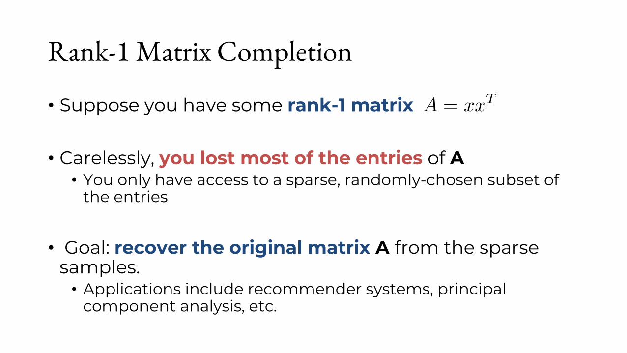
Rank-1 Matrix Completion

• Suppose you have some rank-1 matrix

• Carelessly, you lost most of the entries of A• You only have access to a sparse, randomly-chosen subset of

the entries

• Goal: recover the original matrix A from the sparse samples.• Applications include recommender systems, principal

component analysis, etc.

A = xxT

Matrix Completion as Optimization

• Simplest thing: minimize squared error between model and samples.

• Is this convex?

• We can try to solve this with SGD: randomly choose (i, j) and run

minimizexX

(i,j)2samples

(eTi xxT ej � eTi Aej)

2

xt+1 = xt � 2↵(eTi xxT ej � eTi Aej)(eie

Tj x+ eje

Ti x)

X

(i,j)2samples

(xixj �Aij)2

<latexit sha1_base64="gK6qxinoQZVt+6r1aM2qeU/kwQY=">AAACHXicbVBNTxsxEPUCpWkokJYjF4sIKUgl2k0j0WNaLj2CRD6kbLryOhNwYntX9ixKtNo/wqV/hQuHVhWHXlD/TZ2QAwSeNNLTezOamRenUlj0/X/e2vrGm823pXflrffbO7uVDx87NskMhzZPZGJ6MbMghYY2CpTQSw0wFUvoxpPTud+9BmNFoi9wlsJAsUstRoIzdFJUaYY2U1FeE5/GRzQUmoYIU8wtU6kEWxS0No0EnUZjeky/RrkYF0c/GlGl6tf9BehLEixJlSxxFlX+hsOEZwo0csms7Qd+ioOcGRRcQlEOMwsp4xN2CX1HNVNgB/niu4IeOmVIR4lxpZEu1KcTOVPWzlTsOhXDK7vqzcXXvH6Goy+DXOg0Q9D8cdEokxQTOo+KDoUBjnLmCONGuFspv2KGcXSBll0IwerLL0mnUQ8+1xvnzWrr2zKOEtknB6RGAnJCWuQ7OSNtwskNuSW/yG/vp3fn/fHuH1vXvOXMHnkG7+E/uLuhCg==</latexit>

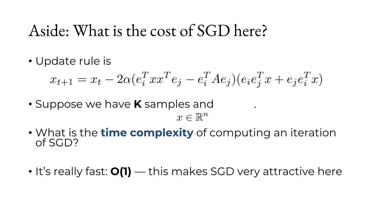
Aside: What is the cost of SGD here?

• Update rule is

• Suppose we have K samples and .

• What is the time complexity of computing an iteration of SGD?

• It’s really fast: O(1) — this makes SGD very attractive here

xt+1 = xt � 2↵(eTi xxT ej � eTi Aej)(eie

Tj x+ eje

Ti x)

x 2 Rn

Demo

A Linear Rate for SGD? Why?

• Variance of the gradient estimator goes to zero over time.

• What is the variance at a particular point x?

• At an optimal point, xxT = A, the variance is zero!

E

���rf(x)���2�=

4

K

X

(i,j)2samples

��(eTi xxT ej � eTi Aej)(eieTj x+ eje

Ti x)

��2

=4

K

X

(i,j)2samples

(eTi xxT ej � eTi Aej)

2((eTj x)2 + (eTi x)

2)

The Role of Variance

• Hypothesis: if the variance becomes small when we get close to the optimum, we converge at a linear rate.

• In fact, we can prove that we get a linear rate if for some C

• Or more generally

E

���rf(x)���2� C

���Ehrf(x)

i���2= C krf(x)k2

Var⇣rf(x)

⌘ C kx� x⇤k2

Can we make this happen for any objective?

• One way to do it:

• In expectation, this is the same since

• And if the samples are Lipschitz continuous with parameter L,

rg(x) = rf(x)�rf(x⇤)

E [rg(x)] = rf(x)�rf(x⇤) = rf(x)� 0

krg(x)k2 = krf(x)�rf(x⇤)k2 L2 kx� x⇤k2

Does this mean we can always get a linear rate?

• Yes! ...for any strongly convex problem where we know the solution.

• Doesn’t seem very useful.

• What if we can approximate the solution? For

• But now our gradients are biased — SGD converges to

rg(x) = rf(x)�rf(x)

x ⇡ x⇤

x not x⇤

Unbiased gradients with approximate solutions

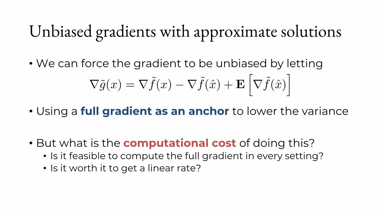
• We can force the gradient to be unbiased by letting

• Using a full gradient as an anchor to lower the variance

• But what is the computational cost of doing this?• Is it feasible to compute the full gradient in every setting?• Is it worth it to get a linear rate?

rg(x) = rf(x)�rf(x) +Ehrf(x)

i

Online and Offline Learning

Two Types of Settings for ML Problems

• Online learning• The training examples arrive one-at-a-time as we are learning• We don’t have access to all the training examples• Not even necessarily a finite training set — new training

examples may be generated in real time in response to e.g.changes in the environment

• Offline learning• We have access to all the training examples upfront• The objective is a finite sum over the given training set

Online Learning

• Have some distribution of training examples, and goal is to

• But we don’t actually have an expression for the distribution

• All we can do is draw samples from it

minimizew Ex⇠distribution [loss(w; x)]

x1, x2, x3, . . .

Advantages of Online Learning

• Online learning generally doesn’t overfit as much• Why? The training distribution is the same as the test

distribution.

• Online learning easily handles new data from the environment

• Systems benefit: we don’t need to materialize the entire training set• Great for scaling up to problems that don’t fit in memory

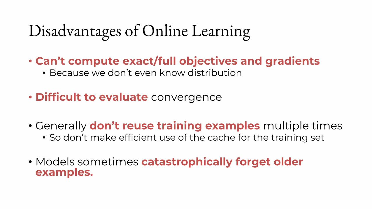
Disadvantages of Online Learning

• Can’t compute exact/full objectives and gradients• Because we don’t even know distribution

• Difficult to evaluate convergence

• Generally don’t reuse training examples multiple times• So don’t make efficient use of the cache for the training set

• Models sometimes catastrophically forget older examples.

Limitations on Online Learning

• 1-D least squares regression: for some distribution μ over R,

• Optimal solution is just the mean, regardless of what μis

minimizexEu⇠µ

1

2(x� u)2

�

x⇤ = Eu⇠µ [u]

Limitations on Online Learning (continued)

• Suppose there were an online learning algorithm that converged at a linear rate for this 1-D least squares problem. Using t samples:

• But we know (from statistics) the lowest-variance estimator for the mean of a distribution, given t samples, is just the sample mean

• Contradiction. No online algorithm can be this good!

E⇥(xt � x

⇤)2⇤= O(�t)

u =1

t

tX

i=1

ut ) Var (u) =1

tVar (ut)

Limitations on Online Learning (continued)

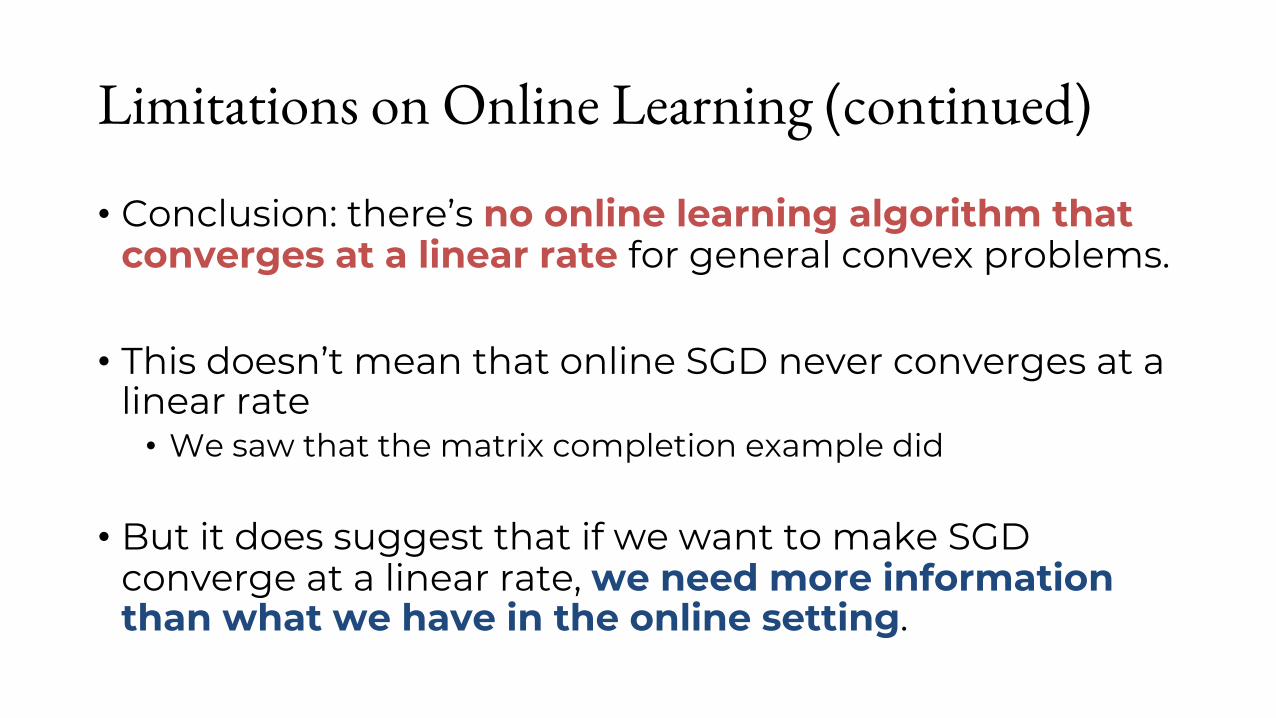
• Conclusion: there’s no online learning algorithm that converges at a linear rate for general convex problems.

• This doesn’t mean that online SGD never converges at a linear rate• We saw that the matrix completion example did

• But it does suggest that if we want to make SGD converge at a linear rate, we need more information than what we have in the online setting.

Aside: Online Learning in Research

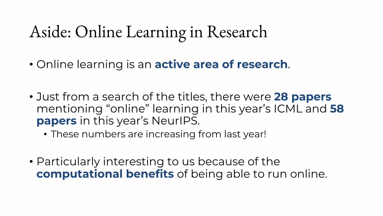
• Online learning is an active area of research.

• Just from a search of the titles, there were 28 papers mentioning “online” learning in this year’s ICML and 58 papers in this year’s NeurIPS.• These numbers are increasing from last year!

• Particularly interesting to us because of the computational benefits of being able to run online.

Offline Learning

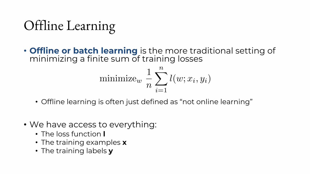
• Offline or batch learning is the more traditional setting of minimizing a finite sum of training losses

• Offline learning is often just defined as “not online learning”

• We have access to everything:• The loss function l• The training examples x• The training labels y

minimizew1

n

nX

i=1

l(w;xi, yi)

Benefits of Offline Learning

• Can compute exact/full objectives and gradients

• Consequence: it’s trivially possible to converge at a linear rate• Just use gradient descent

• Can we leverage this to make an SGD-like algorithm fast?

Stochastic Variance-Reduced Gradient (SVRG)

Recall: Unbiased low-variance samples• From a few slides ago, we were looking at using samples of

the form

• These samples have reduced variance when is close to

• We asked when we could do this, and now we have an answer:• Only in the offline setting!

• Question: how do we use this in an algorithm?

rg(x) = rf(x)�rf(x) +Ehrf(x)

i

x x⇤

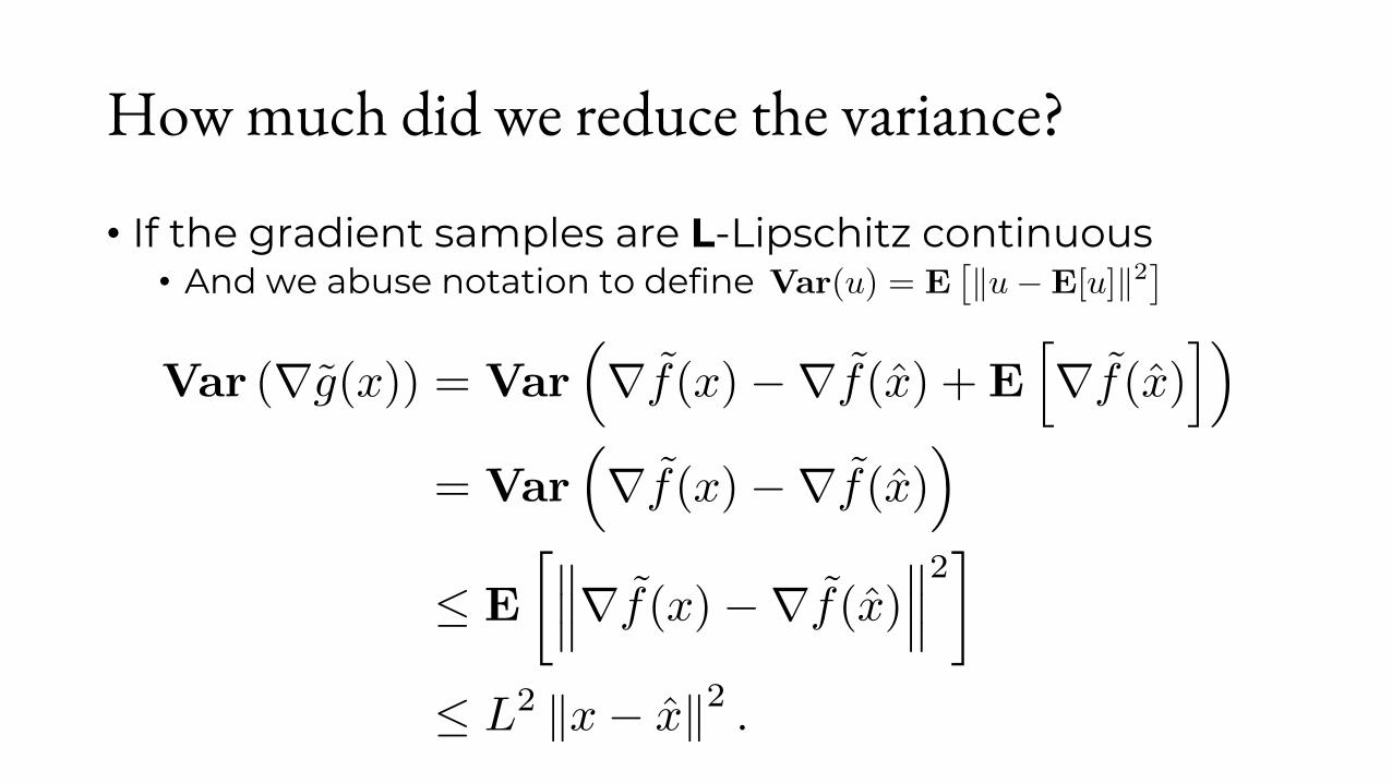
How much did we reduce the variance?

• If the gradient samples are L-Lipschitz continuous• And we abuse notation to define

Var (rg(x)) = Var⇣rf(x)�rf(x) +E

hrf(x)

i⌘

= Var⇣rf(x)�rf(x)

⌘

E

���rf(x)�rf(x)���2�

L2 kx� xk2 .

Var(u) = E⇥ku�E[u]k2

⇤<latexit sha1_base64="HUGHJcpLVcJsATE//jTQwSYmAYs=">AAACLXicbZDLSgMxFIYz9VbrrerSTbAIdWGZEUE3gngBlwq2CjNjyaSZNjRzITkRyjgv5MZXEcFFRdz6GmZqhXr5IfDznXPIOX+QCq7AtodWaWp6ZnauPF9ZWFxaXqmurrVUoiVlTZqIRN4ERDHBY9YEDoLdpJKRKBDsOuifFPXrOyYVT+IrGKTMj0g35iGnBAxqV0+9iEAvCLMWkXldb+ND/E3Ock+wEFzs3WONdya4q30Db3exJ3m3B367WrMb9kj4r3HGpobGumhXn71OQnXEYqCCKOU6dgp+RiRwKlhe8bRiKaF90mWusTGJmPKz0bU53jKkg8NEmhcDHtHJiYxESg2iwHQWG6vftQL+V3M1hAd+xuNUA4vp10ehFhgSXESHO1wyCmJgDKGSm10x7RFJKJiAKyYE5/fJf01rt+EYf7lXOzoex1FGG2gT1ZGD9tEROkcXqIkoekBPaIherUfrxXqz3r9aS9Z4Zh39kPXxCXaIp6M=</latexit><latexit sha1_base64="HUGHJcpLVcJsATE//jTQwSYmAYs=">AAACLXicbZDLSgMxFIYz9VbrrerSTbAIdWGZEUE3gngBlwq2CjNjyaSZNjRzITkRyjgv5MZXEcFFRdz6GmZqhXr5IfDznXPIOX+QCq7AtodWaWp6ZnauPF9ZWFxaXqmurrVUoiVlTZqIRN4ERDHBY9YEDoLdpJKRKBDsOuifFPXrOyYVT+IrGKTMj0g35iGnBAxqV0+9iEAvCLMWkXldb+ND/E3Ock+wEFzs3WONdya4q30Db3exJ3m3B367WrMb9kj4r3HGpobGumhXn71OQnXEYqCCKOU6dgp+RiRwKlhe8bRiKaF90mWusTGJmPKz0bU53jKkg8NEmhcDHtHJiYxESg2iwHQWG6vftQL+V3M1hAd+xuNUA4vp10ehFhgSXESHO1wyCmJgDKGSm10x7RFJKJiAKyYE5/fJf01rt+EYf7lXOzoex1FGG2gT1ZGD9tEROkcXqIkoekBPaIherUfrxXqz3r9aS9Z4Zh39kPXxCXaIp6M=</latexit><latexit sha1_base64="HUGHJcpLVcJsATE//jTQwSYmAYs=">AAACLXicbZDLSgMxFIYz9VbrrerSTbAIdWGZEUE3gngBlwq2CjNjyaSZNjRzITkRyjgv5MZXEcFFRdz6GmZqhXr5IfDznXPIOX+QCq7AtodWaWp6ZnauPF9ZWFxaXqmurrVUoiVlTZqIRN4ERDHBY9YEDoLdpJKRKBDsOuifFPXrOyYVT+IrGKTMj0g35iGnBAxqV0+9iEAvCLMWkXldb+ND/E3Ock+wEFzs3WONdya4q30Db3exJ3m3B367WrMb9kj4r3HGpobGumhXn71OQnXEYqCCKOU6dgp+RiRwKlhe8bRiKaF90mWusTGJmPKz0bU53jKkg8NEmhcDHtHJiYxESg2iwHQWG6vftQL+V3M1hAd+xuNUA4vp10ehFhgSXESHO1wyCmJgDKGSm10x7RFJKJiAKyYE5/fJf01rt+EYf7lXOzoex1FGG2gT1ZGD9tEROkcXqIkoekBPaIherUfrxXqz3r9aS9Z4Zh39kPXxCXaIp6M=</latexit><latexit sha1_base64="HUGHJcpLVcJsATE//jTQwSYmAYs=">AAACLXicbZDLSgMxFIYz9VbrrerSTbAIdWGZEUE3gngBlwq2CjNjyaSZNjRzITkRyjgv5MZXEcFFRdz6GmZqhXr5IfDznXPIOX+QCq7AtodWaWp6ZnauPF9ZWFxaXqmurrVUoiVlTZqIRN4ERDHBY9YEDoLdpJKRKBDsOuifFPXrOyYVT+IrGKTMj0g35iGnBAxqV0+9iEAvCLMWkXldb+ND/E3Ock+wEFzs3WONdya4q30Db3exJ3m3B367WrMb9kj4r3HGpobGumhXn71OQnXEYqCCKOU6dgp+RiRwKlhe8bRiKaF90mWusTGJmPKz0bU53jKkg8NEmhcDHtHJiYxESg2iwHQWG6vftQL+V3M1hAd+xuNUA4vp10ehFhgSXESHO1wyCmJgDKGSm10x7RFJKJiAKyYE5/fJf01rt+EYf7lXOzoex1FGG2gT1ZGD9tEROkcXqIkoekBPaIherUfrxXqz3r9aS9Z4Zh39kPXxCXaIp6M=</latexit>

Var (rg(x)) = Var⇣rf(x)�rf(x) +E

hrf(x)

i⌘

= Var⇣rf(x)�rf(x)

⌘

E

���rf(x)�rf(x)���2�

L2 kx� xk2 .

Var (rg(x)) = Var⇣rf(x)�rf(x) +E

hrf(x)

i⌘

= Var⇣rf(x)�rf(x)

⌘

E

���rf(x)�rf(x)���2�

L2 kx� xk2 .

Var (rg(x)) = Var⇣rf(x)�rf(x) +E

hrf(x)

i⌘

= Var⇣rf(x)�rf(x)

⌘

E

���rf(x)�rf(x)���2�

L2 kx� xk2 .

Is this enough for a linear rate for SGD?

• No, variance at the optimum is reduced, but still not zero!

• Idea: what if we used a sequence of that approaches the optimum?

• Then the variance would go to zero over time! • Intuition: if the variance goes to zero at a linear rate, then SGD

should also converge at a linear rate.

Var (rg(x⇤)) L2 kx⇤ � xk2 .

x

Is this enough? (continued)

• If we have a sequence of that converges to the optimum at a linear rate, then we can use it to reduce the variance of SGD so that it converges to the optimum at a linear rate.

• This also doesn’t seem useful.

• Critical insight: use the iterates of SGD as• So, if SGD converges at a linear rate, then SGD will converge at

a linear rate• Seems circular — but we can make it rigorous

x

x

How often to use full gradient samples?

• Can we use every iteration of SGD as an “anchor” point?

• We could…but this would just be gradient descent.

• Instead, use a full gradient sample periodically• every K iterations of SGD for some hyperparameter K• sometimes called an epoch

rg(x) = rf(x)�rf(x) +Ehrf(x)

i

= rf(x).

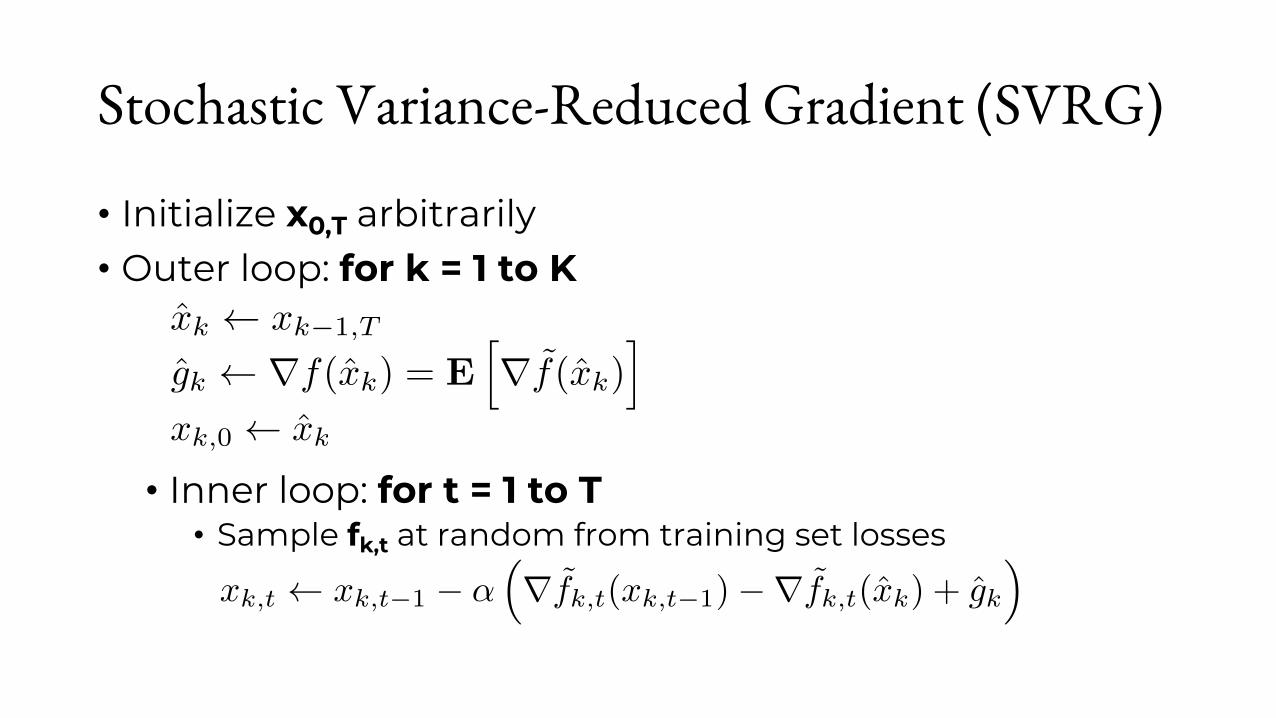
Stochastic Variance-Reduced Gradient (SVRG)

• Initialize x0,T arbitrarily• Outer loop: for k = 1 to K

• Inner loop: for t = 1 to T• Sample fk,t at random from training set losses

xk xk�1,T

gk rf(xk) = Ehrf(xk)

i

xk,0 xk

xk,t xk,t�1 � ↵⇣rfk,t(xk,t�1)�rfk,t(xk) + gk

⌘

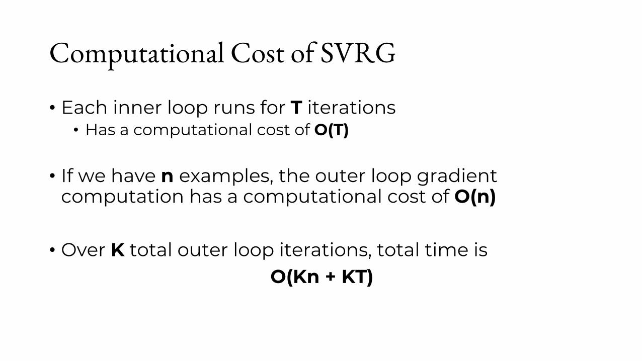
Computational Cost of SVRG

• Each inner loop runs for T iterations• Has a computational cost of O(T)

• If we have n examples, the outer loop gradient computation has a computational cost of O(n)

• Over K total outer loop iterations, total time is O(Kn + KT)

Memory Burden of SVRG

• In addition to the copy of the model that needs to be stored for vanilla SGD, we also need to store• An additional copy of the model vector for the anchor point• An additional vector to store its exact/full gradient

• If the model is of size d, we will need to store a total of 3d numbers• Plus the training set, which is usually much larger

• Takeaway: no significant memory cost to run SVRG

x

Linear Rates for SVRG

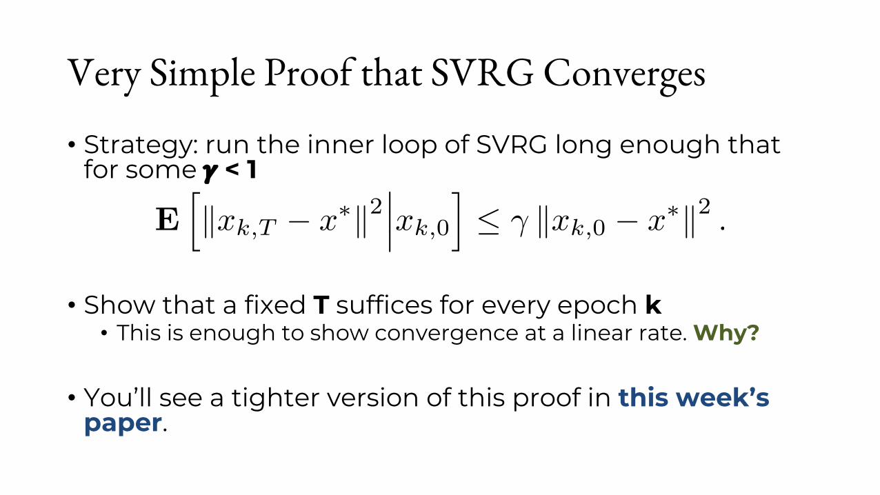
Very Simple Proof that SVRG Converges

• Strategy: run the inner loop of SVRG long enough that for some 𝛾 < 1

• Show that a fixed T suffices for every epoch k• This is enough to show convergence at a linear rate. Why?

• You’ll see a tighter version of this proof in this week’s paper.

Ehkxk,T � x⇤k2

���xk,0

i � kxk,0 � x⇤k2 .

Analysis of an Inner Iterate of SVRG

• Starting with the iterate:

• Let’s simplify it a little by abusing notation to drop the ksubscripts

xk,t = xk,t�1 � ↵⇣rfk,t(xk,t�1)�rfk,t(xk) + gk

⌘

xt = xt�1 � ↵⇣rft(xt�1)�rft(x) +rf(x)

⌘

Analysis (continued)

• Expected distance to the optimum:

• To proceed, need to bound the second order/variance term

E [xt � x⇤|xt�1] = E

���xt�1 � x⇤ � ↵⇣rft(xt�1)�rft(x) +rf(x)

⌘���2����xt�1

�

= kxt�1 � x⇤k2 � 2↵(xt�1 � x⇤)TEhrft(xt�1)�rft(x) +rf(x)

���xt�1

i

+ ↵2E

���rft(xt�1)�rft(x) +rf(x)���2����xt�1

�

= kxt�1 � x⇤k2 � 2↵(xt�1 � x⇤)Trf(xt�1) + ↵2 krf(xt�1)k2

+ ↵2Var⇣rft(xt�1)�rft(x) +rf(x)

���xt�1

⌘

Ehkxt � x⇤k2

���xt�1

i

Analysis (continued)

• Important property: for constant c,

• We can use this to simplify the second order term:

Var (X + c) = Var (X)

Var⇣rft(xt�1)�rft(x) +rf(x)

���xt�1

⌘

= Var⇣rft(xt�1)�rft(x)

���xt�1

⌘

E

���rft(xt�1)�rft(x)���2����xt�1

�

L2 kxt�1 � xk2 2L2 kxt�1 � x⇤k2 + 2L2 kx� x⇤k2

Analysis (continued)

• Substituting this back, we get

• Now we can reduce the first part using strong convexity/Lipschitz

E [xt � x⇤|xt�1] kxt�1 � x⇤k2 � 2↵(xt�1 � x⇤)Trf(xt�1) + ↵2 krf(xt�1)k2

+ ↵2⇣2L2 kxt�1 � x⇤k2 + 2L2 kx� x⇤k2

⌘Ehkxt � x⇤k2

���xt�1

i

Ehkxt � x⇤k2

���xt�1

i kxt�1 � x⇤k2 � 2↵µ kxt�1 � x⇤k2 + ↵2L2 kxt�1 � x⇤k2

+ ↵2⇣2L2 kxt�1 � x⇤k2 + 2L2 kx� x⇤k2

⌘

= (1� 2↵µ+ 3↵2L2) kxt�1 � x⇤k2 + 2↵2L2 kx� x⇤k2

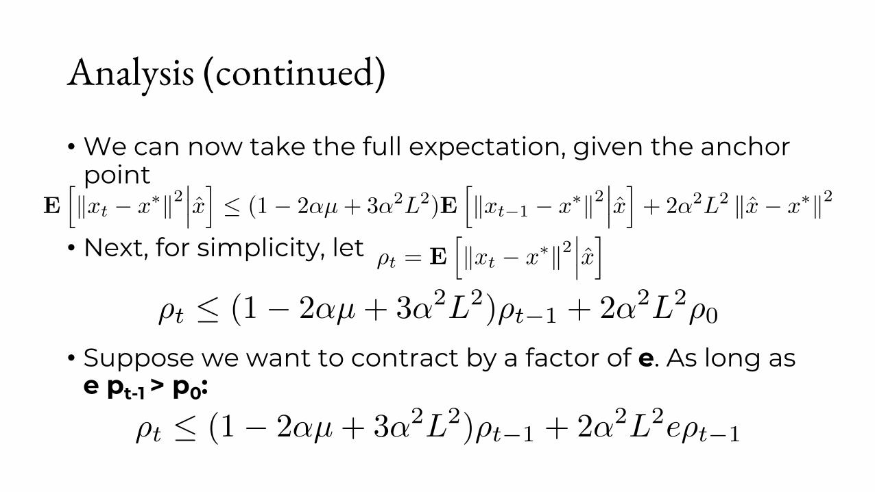
Analysis (continued)

• We can now take the full expectation, given the anchor point

• Next, for simplicity, let

• Suppose we want to contract by a factor of e. As long ase pt-1 > p0:

⇢t = Ehkxt � x⇤k2

���xi

⇢t (1� 2↵µ+ 3↵2L2)⇢t�1 + 2↵2L2⇢0

Ehkxt � x⇤k2

���xi (1� 2↵µ+ 3↵2L2)E

hkxt�1 � x⇤k2

���xi+ 2↵2L2 kx� x⇤k2

⇢t (1� 2↵µ+ 3↵2L2)⇢t�1 + 2↵2L2e⇢t�1

Analysis (continued)

• Now we have

• Setting the step size such that

⇢t (1� 2↵µ+ 3↵2L2)⇢t�1 + 2↵2L2e⇢t�1

(1� 2↵µ+ 5↵2L2e)⇢t�1

↵µ = 5↵2L2e

⇢t ✓1� µ2

5L2e

◆⇢t�1 ) ⇢t

✓1� µ2

5L2e

◆t

⇢0 exp

✓� µ2

5L2et

◆t

⇢0

Analysis (continued)

• Now, this was all contingent upon e pt-1 > p0.

• How many iterations do we need to get there?• Need t such that

• It suffices to pick any

exp

✓� µ2

5L2et

◆ 1

e

t � 5L2e

µ2

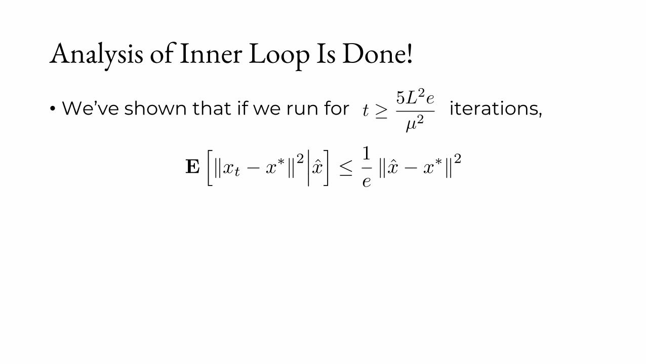
Analysis of Inner Loop Is Done!

• We’ve shown that if we run for iterations,

• In particular, this means that across outer loop iterations,

t � 5L2e

µ2

Ehkxt � x⇤k2

���xi 1

ekx� x⇤k2

Ehkxk+1 � x⇤k2

i 1

eEhkxk � x⇤k2

i

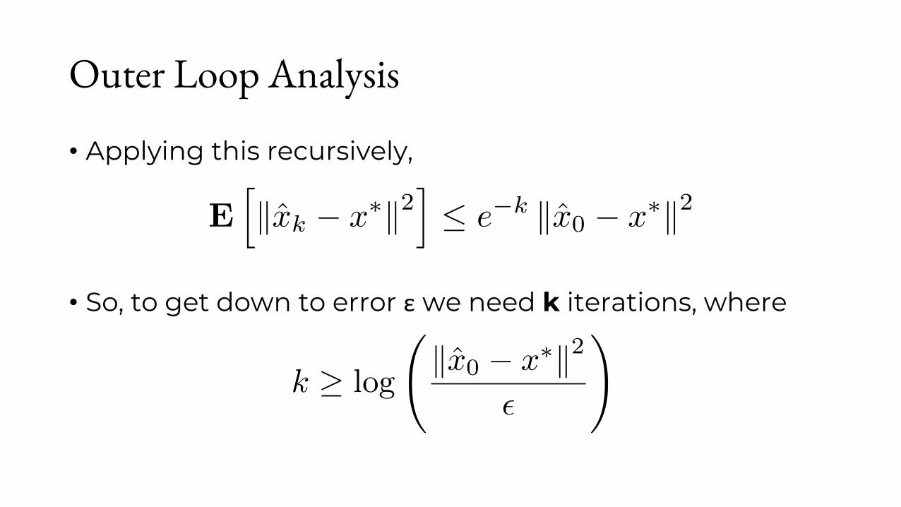
Outer Loop Analysis

• Applying this recursively,

• So, to get down to error ε we need k iterations, where

Ehkxk � x⇤k2

i e�k kx0 � x⇤k2

k � log

kx0 � x⇤k2

✏

!

Bringing it Together

• Total number of stochastic gradient iterations needed is

• This is a linear rate!• Although there’s a much tighter proof in the paper this week

with better dependence on the condition number.

tk � 5L2e

µ2log

kx0 � x

⇤k2

✏

!= O

✓log

✓1

✏

◆◆

Demo

Issues with Variance Reduction

• Computational cost

• Overfitting

• Interaction with other techniques

• Choosing parameters• Metaparameter optimization

Other Methods for Variance Reduction

SAG

• Stochastic average gradient

• At each step, randomly update a single example’s gradient estimate using the current iterate, like SGD

• But, use the sum of all gradient estimates to perform an update

Systems Comparison: SAG vs SVRG

• SAG requires us to store a gradient sample for each training example

• What is the memory cost of doing this, if we have ntraining examples and our model has dimension d?

• Answer: it’s O(nd)

• Compare to SVRG which required O(3d)

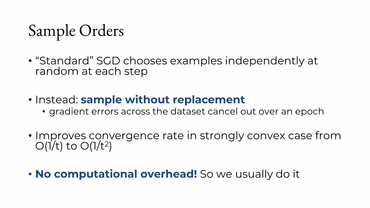
Sample Orders

• “Standard” SGD chooses examples independently atrandom at each step

• Instead: sample without replacement• gradient errors across the dataset cancel out over an epoch

• Improves convergence rate in strongly convex case from O(1/t) to O(1/t2)

• No computational overhead! So we usually do it

Many other variance reduction methods

• SAG• SAGA• SVRG• SDCA – stochastic dual coordinate ascent• Several methods in the distributed setting• Etc.

Questions?

•Upcoming things• Paper Presentation #3 on Monday — read paper before

class• Paper Review #2 due on Monday.