41
Onondaga County Regional Stream Simulation Study Dan Coyle Major Prof. – Dr. Hassett MPS Degree
| Date post: | 20-Dec-2015 |
| Category: |
Documents |
| View: | 217 times |
| Download: | 2 times |

Onondaga County Regional Stream Simulation Study
Dan CoyleMajor Prof. – Dr. Hassett
MPS Degree

OUTLINE
• 1. Introduction
• 2. Study Questions and Objectives
• 3. Model Development
• 4. Results- output charts
• 5. Discussion
Water Resource Management
• Various water processes- water cycle
• Quantity- availability
• Quality- for use
• Resource- value for use
• Damages- problems
• Common to many problems & theory – need for estimates of stream flows

2. Study Questions & Objectives
• Literature search- 2 broad questions
• Model type selection?
• Model development?
• Second iteration is very limited
Categorization of Streamflow Models
• Lumped vs. spatial distributed
• Event versus continuous models
• Theoretical versus empirical
• My choice- lumped, continuous, & empirical
Develop or select model?
• Purposes- needs, ideas, motivations
• Learning curves- cost, time
• Limitations- risks, restrictions
• Assumptions- applicability
• Versatility & ease of use-extensibility
• Time & Money- budget, patience

Study Objective and Development Process
• Create and Evaluate Relatively Simple (and hence Extensible) Streamflow Model(s) Suitable for Central New York Using Readily Available Data Sources
• Utilize Model Development Process Common to Software Engineering Projects

Streamflow as Simulation Problem
• Stream flows- candidate models
• Extract model parameters- simple
• Calibrate parameter values- test
• Predict flows- validate model for ungauged flows

Considerations in Model Development
• A) Limit Streams to Those in National Water Information System (www.usgs.gov)
• B) Meteorological Data from Local National Weather Service Stations) (www.noaa.gov)
• C) Lumped Landuse Descriptors• D) User application container• E) System life cycle• F) Candidate models• G) Base flow separation• H) Application logic

Stream Selection
Name
USGS #
Area
mi2Years Land
Use
Spafford Trib. 04240149800.11 2000-2 Rural
Trib.#6, Below 042379460.32 2000-3 Rural
Meadowbrook 042452363.06 2001-3 Urban
Harborbrook 0424010010.0 2001-3 Suburban
Ley 0424012029.9 2002,3 Urban
Onondaga Cr. Cardiff 04237946
33.9. 2001-4 Rural

3. Model Development -System Life Cycle
• Problem definition- purpose
• Feasibility analysis- possible
• Project design- specifications
• Construction- write, build
• Monitoring- use & test
• Analysis- evaluate
• Control- maintain & adjust
Review of User Application Containers
• MS-Excel- time series, solver, UI
• MS-Access- DB development
• Arc GIS- newer
• Arc View- older
• VB- programming

Candidate Models
• Rainfall Excess - effective precipitation
• Base flow separation from total flow
• Rational Model
• Storages
• Soil Conservation Service Runoff
• Moisture indices & other scaling factors
• Water Balances

Rational Model
Linear Percentage of rainfall
necipitatioctionainFallFraEffectiveRRunOff Pr*

Storages
• Container outflow
servoirtRateConsFlow Re*tan

SCS Curve Numbers
• Runoff from single storm event
)*8.0/()*2.0( 2 SPSPQ
10/1000 rCurveNumbeS
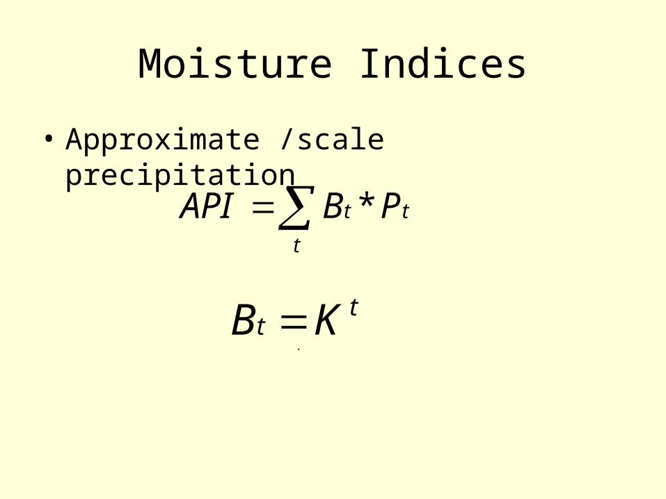
Moisture Indices
• Approximate /scale precipitation
t
t
t PBAPI *
tt KB
.

Water Balance Storage
• For soil moisture flow or evaporation wells
PETPWBS
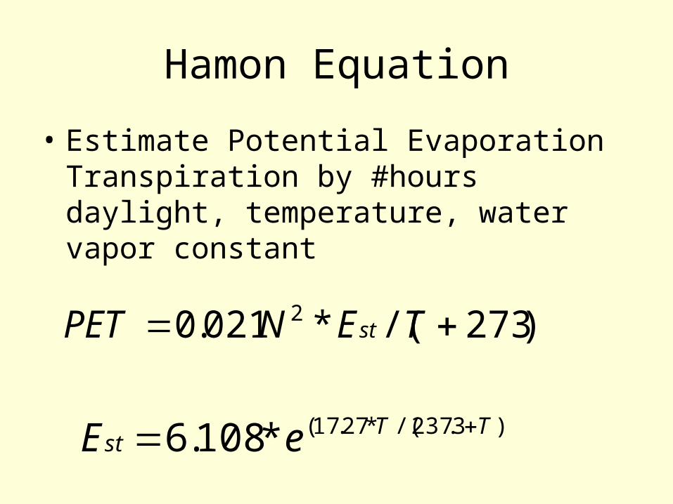
Hamon Equation
• Estimate Potential Evaporation Transpiration by #hours daylight, temperature, water vapor constant
)273/(*021.0 2 TENPET st
)3.237/(*27.17(*108.6 TTst eE

Geographic Averaging
• To weight or scale multiple weather stations
)tan/1/()tan/1( i iii cediscedisWeight

Step Absolute Relative Error
• Solver Optimization Function and averaged over time steps
)/)( observedpredictedobservedARAE
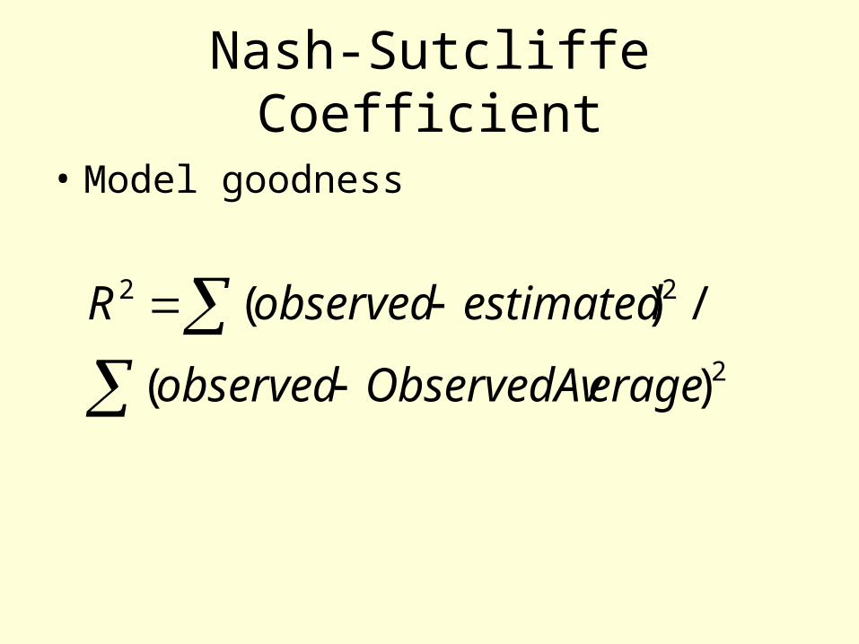
Nash-Sutcliffe Coefficient
• Model goodness
2
22
)(
/)(
erageObservedAvobserved
estimatedobservedR
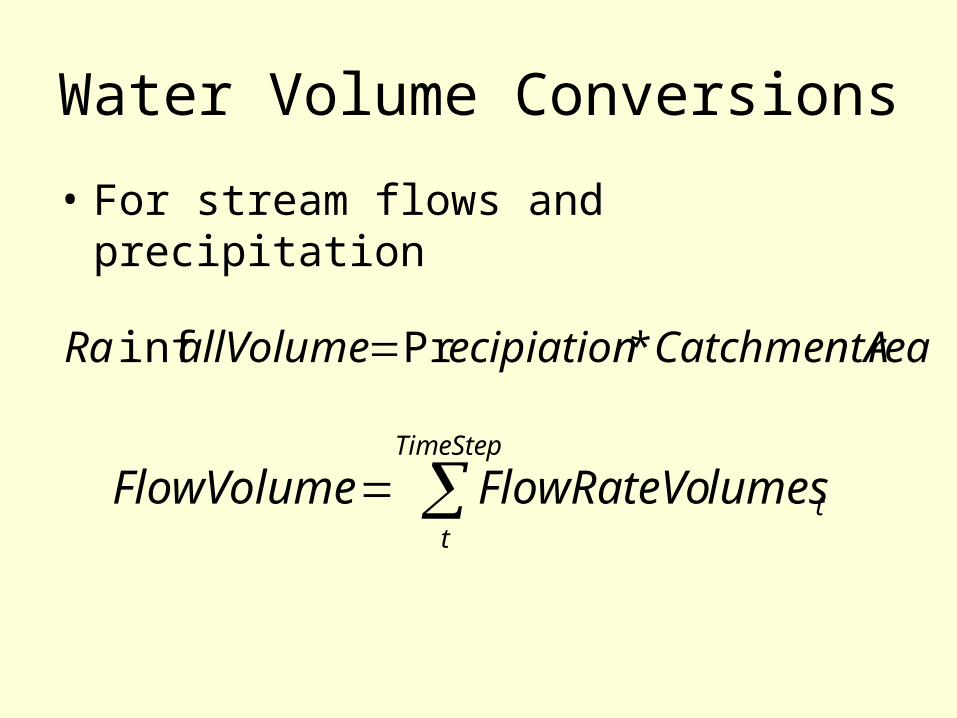
Water Volume Conversions
• For stream flows and precipitation
reaCatchmentAecipiationallVolumeRa *Prinf
TimeStep
ttlumesFlowRateVoFlowVolume

Sample Application logic
• 1) Calculate parameter averages /values
• 2) Calculate slope or store (& subtract from) contribution for base / flows
• 3) Calculate other contributions
• 4) Add up for flow time step
• 5) Check if new average period (step 1)
• 6) Step 2

Model Equations
Sample logic
))((*tan 111
ttt
t
fQuickRunOfflowstoragetRateCons
QFlow
1* tt BaseflowSlopeStepBaseFlow
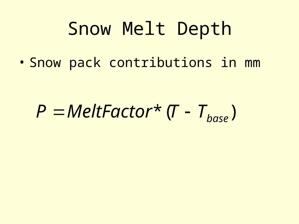
Snow Melt Depth
• Snow pack contributions in mm
)(* baseTTMeltFactorP

4. ResultsTable 2. Overview of models
Model Name
Baseflow Run Off
QuickFlow
PET Years /Season
Monthly slope (sm)
sloped line %rain 11/01-10/03
Monthly store (rm)
reservoir %rain 11/01-10/03
daily slope (sd)
sloped line %rain Summers 2000-4
daily store (rd)
reservoir %rain %rain store Summers 2000-4
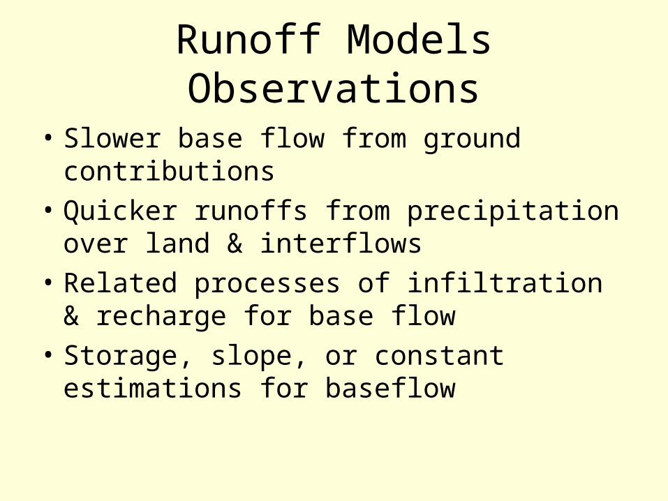
Runoff Models Observations
• Slower base flow from ground contributions
• Quicker runoffs from precipitation over land & interflows
• Related processes of infiltration & recharge for base flow
• Storage, slope, or constant estimations for baseflow

Month Storage, 11/01-10/02
-0.8
-0.6
-0.4
-0.2
0
0.2
0.4
0.6
0.8
1
0 5 10 15
Month
Rech
arge
Fra
ctio
n
Spafford
Below
Meadow
Harbor
Cardiff
Prec.-PET
Figure 9. Monthly model recharge fractions for first year
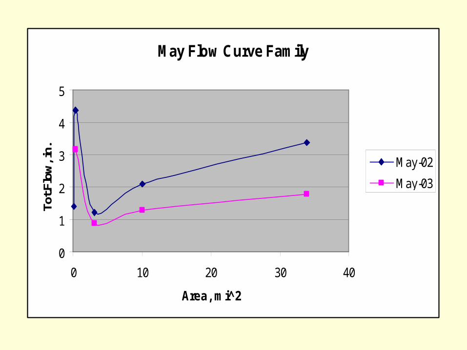
May Flow Curve Family
0
1
2
3
4
5
0 10 20 30 40
Area, mi^2
Tot.F
low
, in.
May-02
May-03

Month Storage
-0.1
0
0.1
0.2
0.3
0.4
0.5
0.6
0.7
0.8
0 10 20 30 40
Area, sq.mi.
Rec
harg
e Fr
actio
n
May-02
May-03
Figure 11. Monthly model recharge fraction and area relational curves

Month Storage
-0.2
0
0.2
0.4
0.6
0.8
1
1.2
1.4
1.6
0 10 20 30 40
Area, mi**2
Dec
ay R
ate
Con
stan
t
May-02
May-03
Figure 8. Monthly model decay rate curves
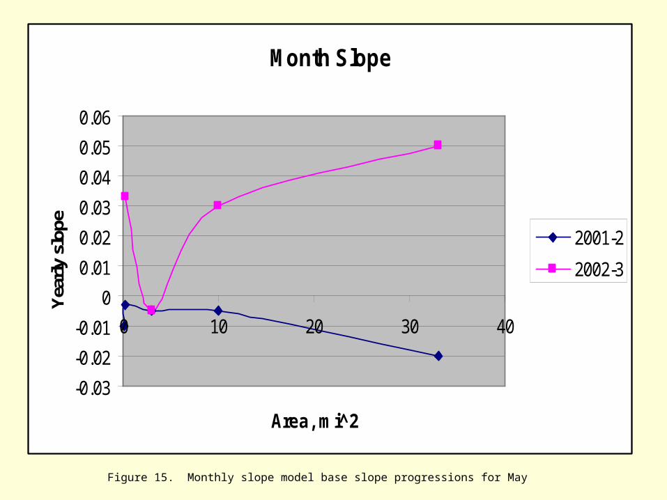
Month Slope
-0.03
-0.02
-0.01
0
0.01
0.02
0.03
0.04
0.05
0.06
0 10 20 30 40
Area, mi^2
Yea
rly
slop
e
2001-2
2002-3
Figure 15. Monthly slope model base slope progressions for May
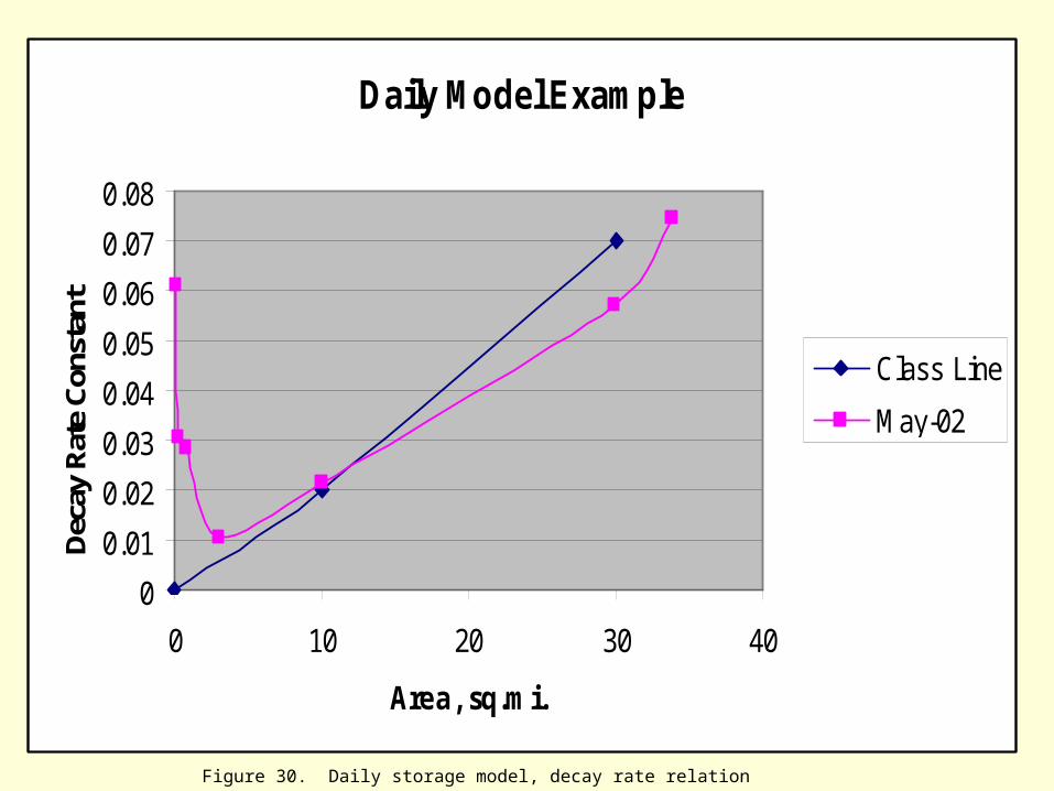
Daily Model Example
0
0.01
0.02
0.03
0.04
0.05
0.06
0.07
0.08
0 10 20 30 40
Area, sq.mi.
Dec
ay R
ate
Con
stan
t
Class Line
May-02
Figure 30. Daily storage model, decay rate relation

Daily Model Example
0
0.1
0.2
0.3
0.4
0.5
0.6
0.7
0.8
0 10 20 30 40
Area, mi^2
Stor
e Re
char
ge F
ract
ion
Class Line
May-02
Figure 31. Daily model reservoir recharge

2002 Flow Predictions
0
50
100
150
200
250
300
-10 0 10 20 30 40
Drainage area, mi**2
% R
elat
ive
Err
or sd-Meadow, 18.2%
sd-Harbor, 12.9%
rd-Harbor, 10.7%
Figure 36. Flow estimates from Tables 6, 8, & 10

Onondaga Creek @ Cardiff
0
10
20
30
40
50
60
9/21/2002
10/1/2002
10/11/2002
10/21/2002
10/31/2002
11/10/2002
Date
Flow
(cfs
) Actual Daily AverageFlow
Simulated Flows
Figure 26. Sample simulation of daily flow

5. Discussion
• Ease of use, vesatile & situational
• PET under/over estimated winter/summer
• 50% Prediction – daily models
• Flow & area relation: rate & recharge
• Approximate PET, recharge factor yearly association
• Runoff spikes underestimated usually
Future
• Shorter parameter average periods
• Finish winter season models with snow melt
• Exponential storage relation?
• Missed key parameter association?
Optimizing function
• Error calculation - minimize
• Relative average error – steady flows
• Monthly step error summaries
• Absolute differences – peaks?
• Nash-Sutcliffe Coefficients?
• Other candidate models?

Conceptual models
• Hydrologic cycle- water budget, possible • Lumped & continuous- set choice • Simplified or approximate- analytical vs.
numerical • Historical or stochastic-simulation vs. synthesis • Physical or mathematical- analog vs. equations • Descriptive or conceptual- observations vs.
theory • Dynamic vs. static


