We study a single-product setting in which a firm can source from two suppliers, one that is unreliable andanother that is reliable but more expensive. Suppliers are capacity constrained, but the reliable supplier
may possess volume flexibility. We prove that in the special case in which the reliable supplier has no flexibilityand the unreliable supplier has infinite capacity, a risk-neutral firm will pursue a single disruption-managementstrategy: mitigation by carrying inventory, mitigation by single-sourcing from the reliable supplier, or passiveacceptance. We find that a supplier’s percentage uptime and the nature of the disruptions (frequent but shortversus rare but long) are key determinants of the optimal strategy. For a given percentage uptime, sourcingmitigation is increasingly favored over inventory mitigation as disruptions become less frequent but longer.Further, we show that a mixed mitigation strategy (partial sourcing from the reliable supplier and carryinginventory) can be optimal if the unreliable supplier has finite capacity or if the firm is risk averse.
Contingent rerouting is a possible tactic if the reliable supplier can ramp up its processing capacity, that is,if it has volume flexibility. We find that contingent rerouting is often a component of the optimal disruption-management strategy, and that it can significantly reduce the firm’s costs. For a given percentage uptime,mitigation rather than contingent rerouting tends to be optimal if disruptions are rare.
Key words : supply uncertainty; dual-sourcing; volume flexibilityHistory : Accepted by Candace A. Yano, operations and supply chain management; received August 1, 2003.This paper was with the author 1 year and 1 month for 4 revisions.
1. IntroductionIn March 2000, lightning caused a fire that shut downthe Philips Semiconductor plant in Albuquerque,New Mexico, for six weeks, leading to a shortage ofcomponents for both Ericsson and Nokia. Accordingto The Wall Street Journal, “company officials say they[Ericsson] lost at least $400 million in potential rev-enue” and “when the company revealed the damagefrom the fire for the first time publicly last July, itsshares tumbled 14% in just hours” (Latour 2001). InFebruary 1997, a fire in a Toyota brake-supplier plantled directly to a two-week shut down of 18 Toyotaplants in Japan, with a resulting cost of $195 mil-lion (Treece 1997). Fires, of course, are not the onlycause of disruptions. Hurricane Mitch caused catas-trophic damage to banana production in many partsof Central America in 1998. It took many growers overa year to recover, leading to a prolonged loss of sup-ply for Dole and Chiquita (Griffy-Brown 2003). Anearthquake in Taiwan severely disrupted supply ofessential components to the personal-computer indus-try leading up to the 1999 holiday season (Burrows1999).It is informative to compare the supply chain strate-
gies of companies and their resulting ability to copewith some of the above-mentioned disruptions. Nokia
lost all of its supply from the Philips plant, but itwas able to temporarily increase production at alter-native suppliers during the disruption, and so suf-fered little financial impact. In contrast, Ericsson hadbeen “weeding out backup suppliers for many parts”and, according to Jan Ahrenbring, Ericsson’s market-ing director for consumer goods, the company con-sequently “did not have a Plan B” (Latour 2001).Ericsson’s single-source strategy caused it to lose over$400 million in potential revenue. A similar con-trast appears in the Hurricane Mitch situation. Chiq-uita, although it lost significant supply, was able totemporarily increase production at some of its other(unaffected) suppliers in the region. Dole had no alter-native suppliers in the region and lost 70% of itsregional supply. Dole suffered a 4% decline in rev-enues (and lost over $100 million) while Chiquitaincreased revenues by 4% in the fourth quarter of 1998(Griffy-Brown 2003). Firms do not need to rely exclu-sively on supply-side tactics during a disruption. Dellwas able to leverage its demand-management capabil-ities to shift demand to alternative products that wereless supply constrained during the 1999 Taiwaneseearthquake disruption, whereas Apple, lacking thesame demand-management capability, was much lessable to cope with the disruption (Griffy-Brown 2003).
Financial mitigation Business interruption In the fourth quarter of 2003, Palm Inc. received a $6.4 million insurance settlement arisinginsurance from an earlier fire at a supplier’s factory.
Operational mitigation Inventory Playmates Toys mitigated the impact of the 2002 west-coast dock disruption by investing in inventoryearlier in the year.
The U.S. Strategic Petroleum Reserve protects the U.S. against interruptions in crude-oil supplies.
Sourcing Nokia’s multiple-supplier sourcing strategy mitigated the impact of the Philips Semiconductor disruptionin 2000.
Chiquita’s multiple-location sourcing strategy mitigated the impact of the 1998 Hurricane Mitch disruption.
Operational contingency Rerouting Nokia responded to the Philips Semiconductor disruption by temporarily increasing production atalternative suppliers.
Chiquita responded to the Hurricane Mitch disruption by temporarily increasing production at alternativelocations.
New Balance responded to the west-coast dock disruption by rerouting ships to the east coast and by airfreighting supplies.
Chrysler responded to the air-traffic disruption in the immediate aftermath of September 11th bytemporarily switching to ground transportation to move components from a U.S. supplier to theDodge Ram assembly plant in Mexico.
Demand management Dell responded to the disruption in memory supply caused by the 1999 Taiwanese earthquake by shiftingcustomer demand to lower-memory personal computers.
Firms can use a number of tactics to manage therisk of disruptions (see Table 1). Mitigation tactics arethose in which the firm takes some action in advanceof a disruption (and so incurs the cost of the actionregardless of whether a disruption occurs). Contin-gency tactics are those in which a firm takes an actiononly in the event a disruption occurs. We note thata contingent-rerouting tactic is viable only if suppli-ers have volume flexibility, that is, the ability to tem-porarily increase their processing capacity. A firm isnot limited to choosing a single tactic, and in manycircumstances a combination of tactics might be theappropriate strategy for managing disruption risk.Mitigation and contingency actions are not free, andtherefore passive acceptance of the disruption riskmay be appropriate in certain circumstances. Passiveacceptance is often the default strategy even when it isnot appropriate. In a recent survey (Poirier and Quinn2004), only 33% of firms responded that they paid“sufficient attention to supply chain vulnerability andrisk mitigation actions.” The focus of this paper ison operational tactics for managing disruption risk.In particular, we focus on the supply-side tactics ofinventory, sourcing, and rerouting.We study a single-product setting in which a firm
can source from two suppliers, one that is unreliableand another that is reliable but more expensive. Sup-pliers are capacity constrained, but the reliable sup-plier may possess volume flexibility. In the specialcase where the reliable supplier has no flexibility,we prove that a risk-neutral firm will pursue apure (i.e., not mixed) disruption-management strat-egy (mitigation by carrying inventory, mitigation by
single-sourcing from the reliable supplier, or pas-sive acceptance) if the unreliable supplier has infi-nite capacity. We find that supplier reliability and thenature of the disruptions (e.g., frequent but short ver-sus rare but long) are key determinants of the optimalstrategy. For a given supplier reliability, as measuredby percentage uptime, sourcing mitigation tends tobe favored over inventory mitigation as disruptionsbecome less frequent but longer. We prove that amixed mitigation strategy (partial sourcing from thereliable supplier and carrying inventory) can be opti-mal if the firm is risk averse or if the unreliablesupplier has finite capacity. Finite capacity amplifiesthe effect of disruptions because the unreliable sup-plier cannot immediately recover from a disruption.We find that this issue of delayed recovery stronglyinfluences the firm’s optimal disruption-managementstrategy.We also characterize the firm’s optimal disruption-
management strategies when the reliable supplierpossesses volume flexibility. We introduce an opera-tional definition of volume flexibility that is charac-terized by the amount of extra capacity that becomesavailable and the speed with which it becomes avail-able. Volume flexibility allows contingent rerouting tobe a tactic. We find that contingent rerouting is oftena component of the optimal disruption-managementstrategy and that it can significantly reduce the firm’scosts. One might expect that rare disruptions wouldfavor a contingency tactic, as contingent costs areincurred only in the event of a disruption. Interest-ingly, for a given supplier reliability, we find that
sourcing mitigation often becomes optimal as disrup-tions become less frequent.The remainder of this paper is organized as follows.
Section 2 surveys the existing literature. A generalmodel is presented in §3. A restricted version of themodel is analyzed in §4. Section 5 returns to the gen-eral model and conclusions are presented in §6. Theproofs for this paper can be found in the online sup-plement (available on the Management Science websiteat http://mansci.pubs.informs.org/ecompanion.html)along with certain technical details that, while impor-tant building blocks, are of secondary importanceto the main results. An unabridged version of thispaper (available from the author upon request) con-tains an extended treatment of the risk-averse alloca-tion decision considered in §5.1. We use the followingmathematical notation in the paper: �x�+ =max�x�0�;�x�− = max�−x�0�; �x� = largest integer less than orequal to x; �x� = smallest integer greater than or equalto x.
2. Literature ReviewWhile the mitigation and contingency frameworkseems like a natural one for supply-uncertainty prob-lems, we are not aware of its usage in the existingsupply-uncertainty literature. Nevertheless, we usethis framework in positioning this paper in relation tothe existing literature.In supply-disruption models, a supplier (or re-
source) is either up or down. When the supplier is upit delivers an order in full and on time, but no ordercan be supplied when it is down. The supply pro-cess is characterized by the interfailure-time distribu-tion and the repair-time distribution. The status of anysupplier is always known to the firm in the disrup-tion literature of which we are aware. The majority ofsupply-disruption papers focus on a single-supplierproblem (Meyer et al. 1979, Bielecki and Kumar 1988,Parlar and Berkin 1991, Parlar and Perry 1995, Gupta1996, Song and Zipkin 1996, Moinzadeh and Aggar-wal 1997, Parlar 1997, Arreola-Risa and De Croix1998). With no alternative source available, inventorymitigation is the only disruption-management strat-egy under consideration in these papers.Parlar and Perry (1996) and Gürler and Parlar
(1997) are, to the best of our knowledge, the onlysupply-disruption papers that consider more than onesupplier. Both papers consider a firm that faces con-stant demand and sources from two identical-cost,infinite-capacity suppliers. The firm faces a fixed costof ordering (although the fixed cost is only incurredonce even if the order is split between suppliers).Interfailure and repair times are exponentially dis-tributed for both suppliers in Parlar and Perry (1996).The authors propose a suboptimal ordering policy
that is solved numerically. Gürler and Parlar (1997)extend the work of Parlar and Perry by consider-ing the case of Erlang-k interfailure times and gen-eral repair times. They develop a cost expression thatneeds to be numerically evaluated and demonstratehow to numerically optimize the inventory for thecase of Erlang-2 interfailure distributions and expo-nential repair times.It is informative to consider the implications of
the infinite-capacity and the identical-cost assump-tions made by Parlar and Perry (1996) and Gürler andParlar (1997) in relation to our mitigation-contingencyframework. The identical-cost assumption removesany downside to sourcing mitigation: the firm is com-pletely indifferent between suppliers if both suppli-ers are up when an order is placed. The combinationof the identical-cost and infinite-capacity assump-tions removes any downside to contingent rerout-ing: if one supplier is down, then the firm has nocost incentive to postpone ordering until that sup-plier is back up, nor is there any limitation onthe order quantity it places with the other supplier.With no downside to sourcing mitigation or con-tingent rerouting, these two papers cannot (and donot purport to) offer any insights into the trade-offsbetween different disruption-management strategies;their contribution lies in the proposed solutions tothe inventory-optimization problem. By consideringfinite-capacity suppliers that differ in cost, our papergoes beyond the existing literature by explicitly mod-eling the trade-offs and limitations inherent in miti-gation and contingency strategies. This then enablesus to provide insights into the structure of an optimaldisruption-management strategy as well as the factorsthat make one strategy preferable over another. Wenote that our paper also allows for uncertain demand.Yield-uncertainty models differ from supply-dis-
ruption models in that there is uncertainty at thetime of order placement as to the fraction of theorder that will be delivered. Much of the literatureon yield uncertainty is focused on single-suppliermodels. Our attention in this survey is restrictedto multiple-supplier models. We refer the interestedreader to Yano and Lee (1995) for a comprehensivereview of the yield-uncertainty literature. There isa limited literature on multiple-sourcing in the con-text of yield uncertainty. Gerchak and Parlar (1990),Agrawal and Nahmias (1997), Gurnani et al. (2000),Dada et al. (2003), Tomlin and Wang (2005), Anupindiand Akella (1993), Parlar and Wang (1993), andSwaminathan and Shanthikumar (1999) all investi-gate supplier diversification in the presence of yielduncertainty, with the latter three being the only onesto consider multiperiod problems. The focus of allthese papers is on inventory and sourcing mitiga-tion. In the single-period problems, contingent rerout-ing does not arise because no sourcing actions are
allowed after uncertainty has been resolved; in themultiperiod problems, the state of a supplier is thesame at the start of each period and so there is noreason to reroute supply.The literature on random capacity has a random
upper bound on production in each period andhas typically focused on single-supplier (or machine)problems, e.g., Ciarallo et al. (1994), Khang andFujiwara (2000), and Bollapragada et al. (2004a, b).One exception is the paper of Kouvelis and Milner(2002), which allows for multiple suppliers in the con-text of outsourcing.All of the multiple-sourcing papers cited above
assume identical lead-time suppliers. Even in theabsence of supply uncertainty, the use of multiplesuppliers can be beneficial if the suppliers differ inlead times and demand is uncertain (see Fukuda1964, Moinzadeh and Nahmias 1988, Scheller-Wolfand Tayur 1998, Sethi et al. 2003, and Feng et al. 2004).We now turn our attention to the literature on flex-
ibility. We refer the reader to Sethi and Sethi (1990),Gerwin (1993), and Suarez et al. (1995) for reviewsof flexibility. Mix flexibility, whereby a resource canproduce multiple products, has been widely studiedin the literature, including in Fine and Freund (1990),Jordan and Graves (1995), Van Mieghem (1998),Kouvelis and Vairaktarakis (1998), Graves and Tom-lin (2003), and Tomlin and Wang (2005). Volume flex-ibility, whereby a resource can temporarily alter itscapacity, has received much less attention.So-called quantity-flexible or options contracts in
the newsvendor contracting literature (e.g., Barnes-Schuster et al. 2002) are somewhat related to volumeflexibility. A firm commits to the purchase of a cer-tain number of units and sets an option reservationquantity. After some demand uncertainty is resolved,the firm has the flexibility of exercising some frac-tion of the reserved options. The firm pays a highermarginal price in total for reserved units than it doesfor committed units. One can think of committedunits as being mitigation inventory and the exercis-ing of reserved options as being a contingent action.A key aspect of these models is that the firm itselfchooses the option reservation quantity, and so thelimitation placed on its contingent action is a directresult of its own earlier decision. Note that there isno supply uncertainty in these models. The defini-tion of volume flexibility as the ability to temporarilyadjust capacity fits more naturally in a multiperiodsetting. Tsay and Lovejoy (1999) is the only multi-period, quantity-flexible contract paper of which weare aware. Again, there is no supply uncertainty intheir model. Tsay and Lovejoy consider a model inwhich a firm can revise previous orders placed witha supplier. Order revisions (upwards or downwards)are bounded, and looser bounds are associated with
higher supplier flexibility. Presumably a supplier withmore volume flexibility can offer a higher degree ofrevision flexibility in the contract.Our paper makes a key contribution to the litera-
ture on flexibility by introducing an operational def-inition of volume flexibility that directly captures asupplier’s ability to temporarily adjust capacity. Ourmodel captures two critical dimensions of volumeflexibility—the magnitude of the capacity increase,and the time it takes for the extra capacity to becomeavailable.Increased attention is being paid to the consid-
eration of risk in operational decisions, especiallyin the context of a single-product newsvendor, e.g.,Eeckhoudt et al. (1995), Agrawal and Seshadri (2000),Schweitzer and Cachon (2000), and Caldentey andHaugh (2004). Sourcing strategies are likely to bestrongly influenced by the firm’s attitudes towardrisk, and so we consider both risk-neutral and risk-averse decision making in this paper. To the bestof our knowledge, the only other supply-uncertaintypaper that considers risk aversion is Tomlin andWang (2005). However, that paper investigates a fun-damentally different setting: a single-period, yield-uncertainty problem in which the firm faces trade-offsbetween mix flexibility and dual-sourcing. Contin-gency actions are not considered in that paper.
3. The ModelIn our model, the firm operates an infinite-horizon,periodic-review inventory systemwith complete back-logging of unmet demand. Demand in period t, Dt ,is drawn from a stationary distribution with strictlypositive support. On-hand inventory at the end of aperiod costs h per unit, and back orders at the end ofa period cost p per unit.The firm has two suppliers (U and R) available
to it. Supplier U is unreliable in the sense that it iseither up or down in a period. We assume that sup-plier U ’s failure and repair transitions are such thatsupplier U can be modeled as a discrete-time Markovprocess. Further assumptions and definitions regard-ing the Markov process are provided at the end ofthis section. Supplier U is assumed to have a con-stant capacity of �u per period. Production is instanta-neous, but there is a transit lead time of L≥ 0 periodsbefore production arrives at the firm. Supplier R iscompletely reliable and also has instantaneous pro-duction and a transit lead time of L periods. The firmchooses an allocation 0 ≤ w ≤ 1, such that it orderswDt in every period from supplier R. For its givenallocation w, supplier R provides sufficient capacity toproduce wDt each period. It cannot, however, instan-taneously ramp up capacity during a disruption tosupplier U . As with Nokia and Chiquita’s suppliers,
we assume that supplier R can potentially providevolume flexibility during a disruption. The function���� denotes the volume flexibility profile; if given �periods’ notice, supplier R can increase its capacity by���� ≥ 0. We assume that ���� is nondecreasing in � ,and we assume that volume flexibility is only madeavailable during a disruption. In particular we willassume the following structure for the volume flex-ibility function: ���� = 0 for � < �r and ���� = � > 0for � ≥ �r . We refer to � as the flexibility magnitudeand �r ≥ 0 as the flexibility response time. Our flexibil-ity profile is then parameterized by ��r� ��. Magnitudeand response time are two key parameters of volumeflexibility: “To replace more than two million poweramplifiers, they [Nokia] asked one Japanese and oneU.S. supplier of the same chip to make millions moreeach. Largely because Nokia is such an important cus-tomer, both took the additional order with only fivedays of lead time” (Latour 2001).Units ordered from supplier U cost cu per unit.
Supplier R charges cr per unit for its normal alloca-tion and charges cf ≥ cr per unit provided from itsvolume-flexible capacity. We assume that cf ≥ cr toreflect that volume flexibility may be associated witha higher marginal cost. We also assume that cr ≥ cuso as to ignore the trivial case where single-sourcingfrom R is clearly optimal. While the motivating exam-ples in the introduction discussed disruptions at sup-pliers external to the firm, our model makes noassumption as to the ownership of either supplier—either or both suppliers could be internal or externalto the firm.All events during period t occur in the following
sequence:• The state of supplier U is observed at the begin-
ning of the period.• Demand is observed.• Ordering decisions are made.• Units produced by a supplier in period t − L
arrive.• Demand is filled (if possible) and holding/back-
order costs are incurred.• Supplier U ’s state transition occurs at the end of
the period.A number of papers (e.g., Kalymon 1971, Song
and Zipkin 1993, Parlar et al. 1995, and Song andZipkin 1996) study Markovian inventory systems inthe context of single-sourcing. The paper by Song andZipkin (1996) is particularly relevant, and we lever-age a number of their results in certain proofs. Thesequence of events above mirrors that proposed bySong and Zipkin, with the exception that we use theconvention (as in Graves 1988, 1999) that demand isobserved before an order is placed, and so in effectour lead time is shorter by one time unit.We define the following variables:
qtu: the order placed on supplier U in period t. Wenote that qtu = 0 if supplier U is down, as there is nopoint in placing an order.
qtr : the order placed on supplier R’s regular capacityin period t. By assumption, this is qtr = wDt where0≤w ≤ 1 is the allocation chosen by the firm.
qtf : the order placed on supplier R’s flexible capac-ity in period t. We note that qtf = 0 if supplier U isup, because flexible capacity is made available onlyduring a disruption.
xt : on-hand inventory level (positive or negative) atthe end of period t.
zt : inventory position (on hand, on order, and intransit) at the end of period t.The ordering and inventory/back-order costs in
period t are then given by
c�qtu� qtr � q
tf �= cuq
tu + crq
tr + cf q
tf and
�C�xt�= p�−xt�+ +h�xt�
+�(1)
respectively. We note that an extension to the case inwhich the firm pays inventory-holding costs for unitsin transit is easily accommodated. We assume thatthere is no cost associated with a volume-flexibilityrequest, and so the firm will request such a capac-ity increase during a disruption. As evidenced bythe Ericsson case, however, a firm may not respondimmediately to a disruption at a supplier. We there-fore assume that the firm does not respond with acapacity-increase request until the start of period �fof a disruption, where �f ≥ 1. For example, if �f = 1,then the firm responds instantaneously to a disrup-tion and places a capacity-increase request at the startof the first period of a disruption, whereas if �f = 2,then the firm doesn’t place a capacity-increase requestuntil the start of the second period. We refer to �f asthe firm’s response time. Given our above assump-tion about the supplier’s volume-flexibility profile,the effective flexible capacity available to the firm inperiod i of a disruption is then 0 if i < �f +�r and � ifi≥ �f + �r . We define the supply chain response timeas �SC = �f + �r .While ordering decisions are tactical in nature, the
allocation decision is strategic. An allocation of w= 0or w = 1 indicates the firm single-sources from sup-plier U or supplier R, respectively. An allocation of0 < w < 1 indicates the firm dual-sources. We notethat even if w = 0, the firm may avail itself of sup-plier R’s volume flexibility if it so chooses. An exten-sion to the case in which supplier R only makesflexibility available if w ≥ wmin > 0 is easily han-dled. Ordering decisions and allocation decisions arelikely made at different levels of the organization,with the allocation decisions made at a higher level.For a given allocation w, we assume that orderingdecisions are made to minimize the long-run average
cost. The firm, however, may exhibit risk aversion inmaking the allocation decision. We consider both amean-variance and a conditional value-at-risk (CVaR)approach in considering risk. Further details regard-ing these approaches are given in §5.1.We now specify our assumptions about supplier U ’s
discrete-time Markov process. Let i = 0�1� ! ! ! ��denote the number of periods (including the currentperiod) for which supplier U has been down. In otherwords, i = 0 if supplier U is up and i = 1� ! ! ! �� ifsupplier U is down and was down in each of theprevious i − 1 periods. The probability of a failure1 − "�0� is assumed to be independent of the num-ber of periods for which U has been up. The prob-ability "�i� of a disruption ending after i periods forwhich U has been down is assumed to depend onlyon i. With these assumptions, supplier U ’s failure andrepair process can be modeled as a Markov chain withstate space i= 0�1� ! ! ! ��. Let i+ denote the state aftera transition from state i ≥ 0; then either i+ = 0, withprobability "�i�, or i+ = i+1, with probability 1−"�i�.We note that for i = 1� ! ! ! ��, "�i� is the probabilitythat a disruption ends after i periods conditional onit having lasted i − 1 periods, i.e., "�i� is the hazardrate for the repair process. We assume that the "�i�are nondecreasing in i for i > 0, i.e., the longer a dis-ruption has lasted the more likely it is to end in thecurrent period, a reasonable model for many disrup-tions. The residual life r�i� at the start of the ith period�i > 0� of a disruption is the remaining number ofperiods until the disruption ends. The mean residuallife r �i� is the expected remaining number of peri-ods until the disruption ends. We note that r �i� ≤1/"�i� and that the increasing hazard rate assump-tion implies that r �i� is nonincreasing in i= 1� ! ! ! ��.Steady-state probabilities for the Markov chain aredenoted by $�i�. The cumulative distribution functionfor the steady-state probabilities is given by F �i� =∑i
�=0$���.The aim of this research is to provide insights into
the factors that influence a firm’s optimal disruption-management strategy. As such, the model should notbe viewed as being designed for decision support. Wehave made a number of simplifying assumptions thatmerit discussion. We ignore any fixed cost of order-ing. In essence, we assume that either fixed costs arenegligible or the underlying base time unit is largeenough that it is sensible to place an order in everyperiod. This latter interpretation is reasonable only solong as the time scale for disruptions is larger thanthe time scale for orders. Our model is appropriatefor firms that order on a daily or weekly basis and areconcerned about disruptions (such as discussed in theintroduction) that may last on the order of weeks oreven months. If fixed costs are such that ordering oncea month is optimal but disruptions are on the scale of
days, then our model is inappropriate. The model isappropriate for monthly ordering as long as the firmis primarily faced with the risk of catastrophic disrup-tions (e.g., Hurricane Mitch), which can cause lossesof supply that may last for months.We assume equal lead times for both suppliers.
In certain circumstances this is a reasonable approx-imation of reality. For example, one of Nokia’s alter-native suppliers to the U.S.-based Philips plant wasalso located in the United States. In other circum-stances, lead times may differ significantly. As men-tioned earlier, it has been established in the literaturethat multiple-sourcing is beneficial if suppliers dif-fer in their lead times. We note that many of thesepapers either make a restrictive assumption that leadtimes differ by one unit (e.g., Fukuda 1964) or elseresort to heuristics (e.g., Moinzadeh and Nahmias1988) or simulation-based optimization (Scheller-Wolfand Tayur 1998) to solve models in which supplierlead times are not consecutive. Feng et al. (2005)show that the optimal policy structure is sensitiveto the consecutive lead-time assumption and thata base-stock policy is no longer optimal when theassumption is relaxed. A goal of our research is toprovide insight into disruption-management strate-gies, and we assume equal lead times so as to removethe nonidentical lead-time motive for dual-sourcing.All of the dual-sourcing, supply-uncertainty paperscited earlier make a similar assumption. A decision-support model might need to incorporate fixed costsand general lead-time suppliers. Solving such a modelwould likely require heuristics or simulation-basedoptimization.In closing this section, we introduce a key lemma
used in a number of later proofs. Consider the fol-lowing inventory system. Demand in each period isstochastic but stationary. The demand random vari-able, denoted by D, has a strictly positive support.Supply is completely reliable, with a guaranteed leadtime of L ≥ 0. Ordering costs are linear but statedependent, with c�0� = cu and c�i� = cf , i > 0. Thestate space and state transitions are identical to thatdescribed above for supplier U . Using a long-runaverage cost criterion, the following results hold forthis inventory system.
Lemma 1. A state-dependent, base-stock policy is opti-mal. The optimal base-stock levels y∗�i� are such thaty∗�i�≤ yM for i≥ 1, where yM minimizes E� �C�y−D�L���,and D�L� is the L-fold convolution of D. y∗�i� is nonincreas-ing in i. If Dt = d with probability 1 (i.e., deterministicdemand), then y∗�0�≥ Ld, y∗�i�= Ld for 0< i≤ icrit, andy∗�i�=−� for i > icrit, where icrit is the maximum valueof i such that r �i� > �cf − cu�/p if r �1� > �cf − cu�/p andicrit = 0 otherwise. If demand is D′
t = kDt where k≥ 0, thenthe optimal base-stock levels and the optimal cost are ky∗�i�and kV ∗ respectively, where V ∗ is the optimal cost whenk= 1.
4. A Restricted ModelIn this section, we focus on a restricted version of themodel in which we assume that (i) the firm is riskneutral, (ii) demand is deterministic (equal to 1 with-out loss of generality), and (iii) supplier U has infinitecapacity. Each of these assumptions will be relaxedin §5.
4.1. The Optimal Ordering PolicyOn a tactical level, the firm needs to determine theoptimal ordering policy. For a given supplier R allo-cation w, the firm must decide the quantity qu�0� toorder from supplier U when it is up, and the quan-tity qf �i� to order from supplier R’s volume flexibilitywhen supplier U is down, i.e., the timing and quan-tity of contingent-rerouting orders.We first consider two extreme cases of volume flex-
ibility: (1) supplier R offers no flexibility, that is,����= 0 for � = 0� ! ! ! ��; and (2) supplier R offersinstantaneous and infinite volume flexibility, that is,����=� for � = 0� ! ! ! �� (in this case we also assumethat the firm responds to a disruption immediately,i.e., �f = 1). We will use the abbreviation II-flexibility torefer to the instantaneous and infinite-flexibility case.
Theorem 1. In the zero-flexibility case, a base-stockpolicy is optimal for orders placed with supplier U whensupplier U is up. Furthermore, y∗
Z�0�w� ≥ L, wherey∗Z�0�w� is the optimal base-stock level. In the II-flexibility
case, a base-stock policy is optimal for orders placed withsupplier U when supplier U is up, and a state-dependentbase-stock policy is optimal for the contingent-reroutingorders when supplier U is down. Furthermore, y∗
I I �0�w�≥L, y∗
I I �i�w� = L for 0 < i ≤ icrit, and y∗I I �i�w�=−� for
i > icrit, where y∗I I �i�w� is the optimal base-stock level in
state i.
Demand in each period is 1 and the firm alwaysorders w from supplier R’s regular capacity. There-fore, in the II-flexibility case, qf �i� = �y∗
I I �i�w� −�z�i−�− �1−w���+ is the rerouting quantity requiredin state i to bring the ending inventory position toat least y∗
I I �i�w�, where i− denotes the state immedi-ately prior to state i and z�i−� is the ending inventoryposition in the prior period. We note that icrit capturesthe trade-off between rerouting and back orders andthat icrit increases as the rerouting cost decreases rel-ative to the back-order cost. The contingent-reroutingpolicy has the following properties.• There exists a threshold value icrit such that if the
disruption has lasted more than icrit periods, then itis optimal to wait until the disruption is over ratherthan to reroute production, that is, qf �i� = 0 for allinventory positions if i > icrit.• If the disruption has lasted less than or equal to
icrit periods and the inventory position is high enoughto prevent a back order L periods from now, then thefirm should not reroute any production.
• If the disruption has lasted less than or equalto icrit periods but the inventory position is not highenough to prevent a back order L periods from now,then the firm should reroute a sufficient quantity toprevent any back orders but not so large a quantity asto build inventory, i.e., it should reroute just enoughto bring its inventory position to L.We now consider the case of partial flexibility or a
delayed firm response. In this case the firm faces con-straints on the quantity it can reroute. In particular,��i− �SC�= 0 for i < �SC and ��i− �SC�= � for i ≥ �SC ,that is, it cannot reroute any quantity if i < �SC andcan reroute at most � per period if i≥ �SC . Recall that�SC = �f + �r .
Theorem 2. In the partial-flexibility (or delayed-firm-response) case, a base-stock policy is optimal for ordersplaced with supplier U when supplier U is up, and a mod-ified state-dependent base-stock policy is optimal for thecontingent-rerouting orders when supplier U is down. Ifthe firm’s inventory position is below the state-dependentbase-stock level y∗
where y∗PF �i�w� = L + n�i��1 − w − ��+ for 0 < i ≤ icrit;
y∗PF �i�w�=−� for i > icrit; n�i� is the maximum integer
n≥ 0 such that cf − cu <M�i�n� and n�i� is defined onlyfor 0 < i ≤ icrit; M�i�n� = �p + h�P�r�i� ≥ n�r�i + n� −hr�i�; and P�r�i� ≥ n� is the probability that the residuallife is at least n periods.
Note that n�i� ≥ 0 as i ≤ icrit and that the n�i�are nonincreasing in i. This theorem states that dur-ing a disruption, the firm attempts to reach a state-dependent base-stock level, but it may not be able todo so because of the volume-flexibility capacity con-straint. We see again that it is not optimal to rerouteif i > icrit. In the II-flexibility case, the optimal base-stock level is L for 0 < i ≤ icrit, the logic being thatcontingent rerouting is perfectly reliable, demand isconstant at 1, and the lead time is L. With partial flex-ibility, this result still holds if �≥ 1−w, the intuitionbeing that if the inventory position is above L andthe flexible capacity has come online, the firm shouldnot yet reroute as it has sufficient capacity to alwayskeep the inventory position at L if it so chooses. Thererouting policy differs, however, if � < 1−w. In thiscase, the extra capacity � is not sufficient to compen-sate for the lost supply 1− w, and so the firm mayreroute lost production before its inventory positionfalls below L so as to prevent future back orders thatresult from the rerouting-capacity constraint. Rerout-ing before the inventory position falls below L meansthat the firm will incur additional inventory costsuntil the inventory position falls below L but willreduce the back orders incurred after that point. Thistrade-off is reflected in the M�i�n� function.
If icrit = 0, then the firm never reroutes lost pro-duction in any state, i.e., the contingency strategyis never used to manage disruption risk. However,icrit > 0 does not imply that a contingency strategyis necessarily used; the optimal base-stock level instate 0 might be sufficient to last beyond icrit, in whichcase rerouting will not occur.
4.2. The Optimal Base-Stock Level WhenSupplier U Is Up
Having characterized the optimal ordering policy,we now proceed to develop the long-run averagecost expression as a function of y�0�w� and w.Recall that y�0�w� is the base-stock level when sup-plier U is up, and w is supplier R’s allocation. Lettingy�0�w�= I0 +L, we will develop the long-run averagecost expression as a function of I0 and w. We will thenoptimize for the base-stock level and supplier R’s allo-cation. In what follows, we will at times use the term“average” in place of “long-run average.” The aver-age cost can be written as
CLRA = cuquLRA�I0�w�+ crq
rLRA�I0�w�+ cf q
fLRA�I0�w�
+hI+LRA�I0�w�+ pI−LRA�I0�w�� (2)
where for a given base stock y�0�w�= I0+L and sup-plier R allocation w,• quLRA�I0�w� is the average quantity per period
sourced from supplier U ,• qrLRA�I0�w� is the average quantity per period
sourced from supplier R’s regular capacity,• q
fLRA�I0�w� is the average quantity per period
sourced from supplier R’s flexible capacity,• I+LRA�I0�w� is the average (nonnegative) on-hand
inventory level, and• I−LRA�I0�w� is the average back order level.We note that quLRA�I0�w�+ qrLRA�I0�w�+ q
fLRA�I0�w�=
1 and that qrLRA�I0�w� = w by definition. Therefore,Equation (2) can be rewritten as
CLRA = cu + �cr − cu�w+ �cf − cu�qfLRA�I0�w�
+hI+LRA�I0�w�+ pI−LRA�I0�w�! (3)
As detailed in Appendix A2 (in the online sup-plement), we can use the renewal reward theoremto derive the following expressions for the averagequantities:
qfLRA�I0�w�=
�∑i=1
qf �i�$�i�� (4)
I+LRA�I0�w�
= I0$�0�+�∑i=1
[I0 − i�1−w�+
i∑k=1
qf �k�
]+$�i�� (5)
I−LRA�I0�w�=�∑i=1
[I0 − i�1−w�+
i∑k=1
qf �k�
]−$�i�! (6)
These long-run average expressions are in fact thesteady-state expected values, and so the long-runaverage cost is equal to the steady-state expected cost.The quantity rerouted in state i, qf �i�, depends on thevolume-flexibility profile. Expressions for q
fLRA�I0�w�,
I+LRA�I0�w�, and I−LRA�I0�w� tailored to the volume-flexibility profile assumed in this paper can be foundin Appendix A2 (in the online supplement).We now define two key variables that influence the
optimal base-stock level:
i∗1 = F −1[
p
p+h
]�
iS =
0� if �cf − cu�$�1� < hF �0�
maximum i such that �cf − cu�$�i�≥ hF �i− 1��otherwise.
Both i∗1 and iS refer to numbers of periods and cap-ture different trade-offs facing the firm. The trade-off between inventory and back orders is capturedby i∗1. We note that i∗1 increases as inventory becomescheaper relative to back orders. One can think of i∗1as a newsvendor-type variable. In fact, as shownbelow, i∗1 is the number of periods’ coverage providedby the optimal base stock in the zero-flexibility case.The trade-off between inventory and rerouting is cap-tured by iS . It is cheaper for the firm to carry an addi-tional unit of inventory than to reroute in period i ofa disruption if i ≤ iS . Note that iS increases as inven-tory becomes cheaper relative to rerouting. As notedearlier, the trade-off between back orders and rerout-ing is captured by icrit. For a given allocation w, theoptimal base-stock level y∗�0�w�= I∗0 �w�+ L is speci-fied by the following theorem for all values of �f , �r ,and �. Recall that �SC = �f + �r .
Theorem 3. If w= 1, then I∗0 �w�= 0. If w< 1, then
maximum I0 such that(�h+p�F �T �I0�w��−pF �N �I0�w�−1�
−�cf −cu�$�N�I0�w��
)≥0�
otherwise�
and
T �I0�w�=⌊
I01−w
⌋�
N �I0�w�=
�SC − 1+⌈��SC − 1��1−w�− I0
�− �1−w�
⌉�
T �I0�w� < �SC − 1
T �I0�w�+ 2� T �I0�w�≥ �SC − 1�
i�w�=⌊���SC − 1��1−w�− ��− �1−w���icrit − �SC��
+
�1−w�
⌋!
4.3. The Optimal Sourcing StrategyWe now proceed to determine the optimal sourc-ing strategy. Recall that w∗ = 1 implies that the firmsingle-sources from supplier R, 0<w∗ < 1 implies thefirm dual-sources, and w∗ = 0 implies the firm single-sources from supplier U .We first consider the two extreme cases of volume
flexibility: II-flexibility and zero flexibility.
Theorem 4. Single-sourcing is optimal in both cases,that is, w∗
I I ∈ �0�1� and w∗Z ∈ �0�1�. If single-sourcing
from supplier U is optimal for the zero-flexibility case,then it is also optimal for the II-flexibility case, i.e.,w∗
Z = 0⇒w∗I I = 0. If single-sourcing from supplier R is
optimal for the II-flexibility case, then it is also optimal forthe zero-flexibility case, i.e., w∗
I I = 1⇒w∗Z = 1.
This theorem tells us that an extreme sourcing strat-egy is optimal at both ends of the flexibility profile.Does this extreme result hold for intermediate flexi-bility regimes? To answer this question, we now con-sider the case in which supplier R offers only partialflexibility and/or the firm does not respond instan-taneously to a disruption. Define E1�i� =
∑i�=0 �$���,
E2�i� =∑�
�=i+1 �$���, K1�i� = E1�i�− iF �i�, and K2�i� =E2�i�−i�1−F �i��. The optimal sourcing strategy for thecase of partial flexibility (or delayed firm response) isgiven in the following theorem.
Theorem 5. If i∗1 > icrit (that is, rerouting is too expen-sive relative to inventory), then volume flexibility is neverused and single-sourcing is optimal, i.e., w∗ ∈ �0�1�, with
w∗ = 0 ⇐⇒ cr ≥ cu −hK1�i∗1�+ pK2�i
∗1�! (7)
If i∗1 ≤ icrit, but �SC > icrit (that is, the supply chain responsetime is too slow and/or rerouting is too expensive rela-tive to back orders), then volume flexibility is never usedand single-sourcing is optimal, i.e., w∗ ∈ �0�1�, with Equa-tion (7) again determining the optimal supplier choice. Ifi∗1 ≤ icrit, and �SC ≤ icrit (that is, rerouting is a viable optionboth in terms of cost and supply chain response time), thenthe optimal sourcing strategy depends on both the supplychain response time �SC and the flexibility magnitude � inthe manner specified by Table 2.
If dual-sourcing is optimal, then w∗ ≥ �1− ��+, thatis, the firm chooses an allocation such that the magni-tude of flexibility is sufficient to prevent (if it choosesto) any further increase in back orders once flexi-bility becomes available. We segmented the sourcingstrategy by the flexibility parameters, as this gavethe cleanest segmentation. Of course, other parame-ters influence the optimal allocation, either indirectlythrough their influence on i∗1, iS , and icrit, or directlythrough their influence on the purchasing costs. Innumerical tests, the behavior of w∗ with respect tomodel parameters was as one would expect, e.g., sup-plier R’s allocation was increasing in the back-ordercost p and inventory-holding cost h and decreasing inits relative cost cr/cu and supplier U ’s reliability [asmeasured by $�0�, the steady-state probability that Uis up]. Supplier R’s allocation was found to be par-ticularly sensitive to relative cost and reliability. Wealso found that supplier R’s allocation decreased inthe level of flexibility it offered, as flexibility allowsthe firm to engage in contingent rerouting rather thanmitigation sourcing (i.e., routine sourcing from sup-plier R). Suppliers are therefore advised to be cautiousabout offering flexibility.
4.4. The Optimal Disruption-ManagementStrategy
Having characterized the optimal rerouting, inven-tory, and sourcing decisions for the firm, we nowproceed to use these results to characterize the set
Table 2 Optimal Sourcing Strategy When i∗1 ≤ icrit and �SC ≤ icrit
Flexibility magnitude
Response time Low (i.e., � < 1) High (i.e., �≥ 1)
Intermediate response Single- or dual-source Single- or dual-source(i.e., �SC > iS + 1) w ∗ = 0 or 1− �≤ w ∗ ≤ 1 0≤ w ∗ ≤ 1
Fast response Single- or dual-source Single-source(i.e., �SC ≤ iS + 1 w ∗ ∈ 0�1− ��1� w ∗ ∈ 0�1�
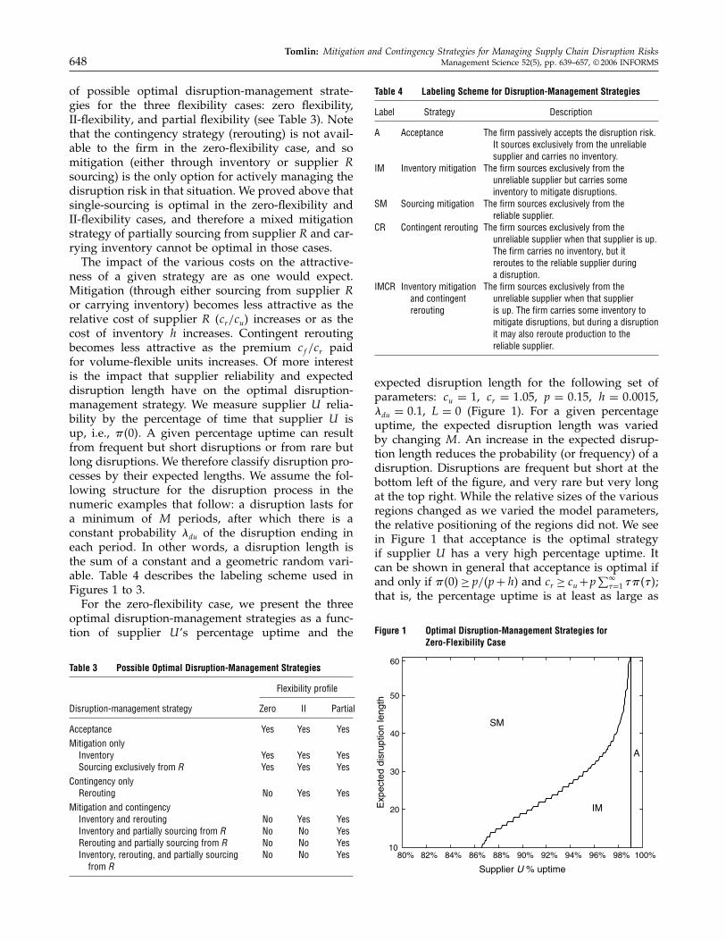
of possible optimal disruption-management strate-gies for the three flexibility cases: zero flexibility,II-flexibility, and partial flexibility (see Table 3). Notethat the contingency strategy (rerouting) is not avail-able to the firm in the zero-flexibility case, and somitigation (either through inventory or supplier Rsourcing) is the only option for actively managing thedisruption risk in that situation. We proved above thatsingle-sourcing is optimal in the zero-flexibility andII-flexibility cases, and therefore a mixed mitigationstrategy of partially sourcing from supplier R and car-rying inventory cannot be optimal in those cases.The impact of the various costs on the attractive-
ness of a given strategy are as one would expect.Mitigation (through either sourcing from supplier Ror carrying inventory) becomes less attractive as therelative cost of supplier R �cr/cu� increases or as thecost of inventory h increases. Contingent reroutingbecomes less attractive as the premium cf /cr paidfor volume-flexible units increases. Of more interestis the impact that supplier reliability and expecteddisruption length have on the optimal disruption-management strategy. We measure supplier U relia-bility by the percentage of time that supplier U isup, i.e., $�0�. A given percentage uptime can resultfrom frequent but short disruptions or from rare butlong disruptions. We therefore classify disruption pro-cesses by their expected lengths. We assume the fol-lowing structure for the disruption process in thenumeric examples that follow: a disruption lasts fora minimum of M periods, after which there is aconstant probability "du of the disruption ending ineach period. In other words, a disruption length isthe sum of a constant and a geometric random vari-able. Table 4 describes the labeling scheme used inFigures 1 to 3.For the zero-flexibility case, we present the three
optimal disruption-management strategies as a func-tion of supplier U ’s percentage uptime and the
Table 3 Possible Optimal Disruption-Management Strategies
Flexibility profile
Disruption-management strategy Zero II Partial
Acceptance Yes Yes YesMitigation only
Inventory Yes Yes YesSourcing exclusively from R Yes Yes Yes
Contingency onlyRerouting No Yes Yes
Mitigation and contingencyInventory and rerouting No Yes YesInventory and partially sourcing from R No No YesRerouting and partially sourcing from R No No YesInventory, rerouting, and partially sourcing No No Yes
from R
Table 4 Labeling Scheme for Disruption-Management Strategies
Label Strategy Description
A Acceptance The firm passively accepts the disruption risk.It sources exclusively from the unreliablesupplier and carries no inventory.
IM Inventory mitigation The firm sources exclusively from theunreliable supplier but carries someinventory to mitigate disruptions.
SM Sourcing mitigation The firm sources exclusively from thereliable supplier.
CR Contingent rerouting The firm sources exclusively from theunreliable supplier when that supplier is up.The firm carries no inventory, but itreroutes to the reliable supplier duringa disruption.
IMCR Inventory mitigation The firm sources exclusively from theand contingent unreliable supplier when that supplierrerouting is up. The firm carries some inventory to
mitigate disruptions, but during a disruptionit may also reroute production to thereliable supplier.
expected disruption length for the following set ofparameters: cu = 1, cr = 1!05, p = 0!15, h = 0!0015,"du = 0!1, L = 0 (Figure 1). For a given percentageuptime, the expected disruption length was variedby changing M . An increase in the expected disrup-tion length reduces the probability (or frequency) of adisruption. Disruptions are frequent but short at thebottom left of the figure, and very rare but very longat the top right. While the relative sizes of the variousregions changed as we varied the model parameters,the relative positioning of the regions did not. We seein Figure 1 that acceptance is the optimal strategyif supplier U has a very high percentage uptime. Itcan be shown in general that acceptance is optimal ifand only if $�0�≥ p/�p+h� and cr ≥ cu+p
∑��=1 �$���;
that is, the percentage uptime is at least as large as
Figure 1 Optimal Disruption-Management Strategies forZero-Flexibility Case
Figure 2 Optimal Disruption-Management Strategies for II-FlexibilityCase �cf = 2�5cr
80% 82% 84% 86% 88% 90% 92% 94% 96% 98% 100%10
20
30
40
50
60
Supplier U % uptime
Exp
ecte
d di
srup
tion
leng
th
SM
IM
CR
A
a newsvendor fractile and the reliable-supplier costis at least as large as the unreliable-supplier costplus expected back-order costs. Acceptance is there-fore favored in environments of high supplier relia-bility, with the definition of “high” being dependenton the costs of mitigation and the cost of back orders.For a given percentage uptime, inventory mitigationis favored if disruptions tend to be short (and hencemore frequent), but sourcing mitigation is favored ifdisruptions tend to be long (and hence less frequent).The reason that sourcing mitigation is favored overinventory mitigation as disruptions become longerand less frequent is that more inventory is requiredin such environments, and so inventory mitigationbecomes less attractive. Carrying high amounts ofinventory for rare events is not an attractive strategy if
Figure 3 Optimal Disruption-Management Strategies for II-FlexibilityCase �cf = 1�25cr
80% 82% 84% 86% 88% 90% 92% 94% 96% 98% 100%10
20
30
40
50
60
Supplier U % uptime
Exp
ecte
d di
srup
tion
leng
th
IMCR
CR
SM
another mitigation option (in our case, sourcing fromsupplier R) is available.Mitigation is the only available strategy in the zero-
flexibility case, but contingent rerouting is availablewhen supplier R provides volume flexibility. Whilecontingent-rerouting costs more than regular pro-duction, i.e., cf ≥ cr > cu, the benefit of the contin-gency strategy is that the firm only incurs the highercontingent-rerouting cost during a disruption. Withmitigation strategies, the firm incurs a cost (eitherinventory or the higher supplier R sourcing cost)even when supplier U is up. One might thereforeexpect that a contingency strategy would be preferredif disruptions are rare events, i.e., if the probabil-ity of supplier failure is very low. The story, how-ever, is somewhat more nuanced than this. Using thesame parameters as above, we present the optimaldisruption-management strategy for the II-flexibilitycase when the relative rerouting cost is very high,i.e., cf = 2!5cr (see Figure 2) and when it is lower,i.e., cf = 1!25cr (see Figure 3). We see from Figure 2that a contingency strategy can be optimal even fora very high rerouting cost. As the rerouting costdecreases, contingent rerouting (either in isolation orcombined with inventory mitigation) is preferred overa larger region. Again, while the relative sizes ofthe various regions vary as parameters change, therelative positioning of the regions does not. Contin-gent rerouting becomes less attractive as supplier U ’spercentage uptime decreases (for a given expecteddisruption length), the reason being that the bene-fit of the contingent-rerouting strategy decreases asthe higher contingency-rerouting cost is incurred agreater percentage of the time. Sourcing mitigationis never optimal in the II-flexibility case if cf = cr ,as contingent rerouting is no more expensive thanmitigation sourcing but is incurred less frequently.Contingent rerouting also becomes less attractive asthe expected disruption length increases (for a givensupplier U percentage uptime). Eventually mitiga-tion, either through inventory or routine sourcingfrom supplier R, becomes optimal as the disrup-tion length increases. This indicates that a mitiga-tion strategy is preferred to the contingency strategywhen the frequency of disruption is very low, a resultthat might seem counterintuitive. The reason for thisagain lies with the fraction of time the contingentcost is incurred. Whereas the percentage downtime isconstant for a given percentage uptime, the percent-age of time spent rerouting is not constant; it dependson the expected disruption length. Recall from The-orems 1 and 2 that the use of contingent reroutingdepends on the residual life of a disruption. As theexpected disruption length increases, the firm spendsmore time in states in which rerouting is optimal, andhence the relative benefit of the contingency strategy
decreases until a point is reached at which mitigationbecomes optimal.We see from Figures 1, 2, and 3 that the optimal
disruption-management strategy depends on whethervolume flexibility is available. Volume flexibility en-ables a contingency strategy, and a contingency strat-egy can be preferable to a mitigation (or acceptance)strategy. Does volume flexibility significantly reducea firm’s long-run average costs? In Figures 4 and 5we illustrate the relative cost reduction achieved byII-flexibility (over zero flexibility) as a function of sup-plier U ’s percentage uptime and the expected dis-ruption length using the same parameters as in Fig-ures 2 and 3. The relative cost reduction is zero inregions where contingent rerouting is not an optimalstrategy, and so the three-dimensional surface graphsreflect the regions illustrated in Figures 2 and 3. In theregions where contingent rerouting is optimal, we seethat II-flexibility can result in a cost reduction of 3%–4%. This is a reduction in the overall costs (includingprocurement) and not simply a reduction in inven-tory and back-order costs. As such, this is a significantreduction. In fact, if one could make supplier U per-fectly reliable in the zero-flexibility case, then the max-imum savings from doing this would be 4.76% (as thereliable-supplier cost of 1.05 places an upper boundon the possible long-run average cost when supplierU is unreliable). We therefore see that the availabil-ity of II-flexibility is almost as beneficial as perfectsupplier reliability even when the cost of exercisingthat flexibility is expensive. Note that as the rerout-ing cost decreases to cf = cr , the relative cost reduc-tion increases and the region in which those reductionsoccur also grows.II-flexibility is unlikely to exist for most firms,
either because suppliers do not offer it (e.g., Nokia’ssuppliers took five days to increase production) orbecause the firm does not respond instantaneously toa supplier disruption (e.g., Ericsson did not respond
Figure 4 Cost Reduction Arising from II-Flexibility �cf = 2�5cr
Figure 5 Cost Reduction Arising from II-Flexibility �cf = 1�25cr
with contingent-rerouting requests until several ofweeks after the disruption). Partial flexibility is a morereasonable model of the reality most firms face. Itis of interest to understand how quickly the bene-fits of II-flexibility decrease as flexibility decreases.Recall that we parameterize supplier flexibility by themagnitude � and the response time �r , and that flex-ibility decreases as the magnitude decreases or asthe response time increases. In Figure 6 we presentexchange curves (or contours) for magnitude andresponse time for three different expected disruptionlengths (expressed in numbers of periods). The con-tours specify the percentage (from 10% to 90%) of theII-flexibility benefit that is delivered by partial flexi-bility. An uptime percentage of 97% was chosen andthe same cost parameters as in Figure 3 were used.Two observations are noteworthy, as they were
observed in many other numeric examples. First, forvery high magnitudes, the performance of partialflexibility is more sensitive to response-time degra-dation when the expected disruption length is low.This reflects the fact that the extra capacity is oflittle value if a disruption is nearly over by thetime capacity becomes available. Second, the trade-off between magnitude and response is more extremewhen disruptions are short (and hence more frequent)in nature: for high response times, a large increase inmagnitude is needed to offset a small degradation inresponse time (again this reflects the fact that magni-tude is of little value if it becomes available when adisruption is nearly over), but for low response times,a very small increase in magnitude offsets a largedegradation in response time (this reflects the fact thatinventory can compensate for an increase in responsetime, and as discussed above, carrying inventory isrelatively less expensive when disruptions are shortand frequent rather than long and rare). Measur-ing response time relative to the expected disrup-tion length, we found that for very high magnitudes
Figure 6 Partial Flexibility Exchange Curves for a 97% Uptime Percentage as Expected Disruption Length (EDL) Increases
1.00 0.75 0.50 0.25 00
5
10
15
20
25
30
35
40
Flexibility magniture
Fle
xibi
lity
resp
onse
tim
e
EDL = 7
1.00 0.75 0.50 0.25 00
5
10
15
20
25
30
35
40
Flexibility magnitude
EDL = 14
1.00 0.75 0.50 0.25 00
5
10
15
20
25
30
35
40EDL = 28
Flexibility magniture
10%,
20%,
...,
90%
Contours
Contours
Contours
the performance of partial flexibility is more sensi-tive to the relative response time when the expecteddisruption length is greater. This observation againreflects the fact that inventory can compensate for anincrease in response time. As inventory is unattractivewhen disruptions are long and rare, inventory is lesseffective at compensating for an increase in relativeresponse time.In closing we mention that all the above figures
assume instantaneous firm response time, i.e., �f = 0.For a noninstantaneous firm response time, the flex-ible capacity becomes available after the sum of thefirm’s response time and the supplier’s response time,i.e., �f + �r , and so one can still use the above figuresby interpreting the response time to be the combinedresponse time.
4.5. The Impact of Misestimating SupplierReliability
Our model assumes that the firm can accurately char-acterize the reliability of a supplier. In practice, a firmmay have to estimate a supplier’s reliability whenchoosing a disruption-management strategy. We con-ducted a numeric study to investigate the impactof parameter misestimation on the long-run averagecost. We assumed the same disruption structure asin the earlier numeric examples, namely a disruptionlength that is the sum of a constant plus a geomet-ric random variable. Recall that the model assumes
a constant probability of failure when supplier U isup. In our study, we focused on the misestimationof the failure probability, and assumed that the firmcould accurately estimate repair probabilities. Thereis a one-to-one relationship between the failure prob-ability and supplier U ’s uptime percentage (for agiven disruption process), and we therefore use theuptime percentage as the parameter that the firm esti-mates. For each problem instance we assumed thatthe true uptime percentage was 97% but that thefirm’s estimate of the uptime percentage could devi-ate from the true value by as much as ±3%. We solvedfor the firm’s optimal strategy given its estimate ofthe uptime percentage and then calculated the actuallong-run average cost of the resulting strategy giventhe true uptime percentage. The impact of uptimemisestimation was then measured by the percentageincrease in long-run average cost resulting from theincorrect estimate. We fixed the holding cost h at0.0015, the unreliable-supplier cost cu at 1, the flexi-bility premium cf /cr at 1.05, the firm response time�f at 1, and the lead time L at 1. We conducted a full-factorial study for the parameters listed in Table 5.In Table 6 we present the percentage cost increase
(over all the relevant instances) resulting from sup-plier uptime misestimations for zero flexibility andII-flexibility �� = 1� �r = 0�. While misestimation cansignificantly increase costs (with the cost increase
being as high as 7.36% in one case), II-flexibility sig-nificantly reduces the negative effect of misestimation.In addition to reducing a firm’s long-run average cost,volume flexibility results in a disruption-managementstrategy that tends to be more robust to parametermisestimation. We observed the following results inthe numeric study. The cost increase due to overesti-mation was typically higher than the cost increase dueto underestimation. There were, however, instancesfor which the reverse was true—underestimationtended to result in a larger cost increase than overes-timation when the back-order cost was low. The costincrease arising from misestimation increased as theback-order cost increased and as the expected dis-ruption length increased. The cost increase typicallydecreased as the flexibility magnitude increased andas the flexibility response time decreased, but therewere some instances in which flexibility amplified themisestimation penalty.
5. Extensions to the Restricted ModelWe now relax three key assumptions of the restrictedmodel: risk neutrality, deterministic demand, and infi-nite supplier U capacity. Unless otherwise stated, weassume instantaneous lead times �L = 0� in all thatfollows.
5.1. Risk Aversion in the Allocation DecisionUp to this point we have assumed that the allocationdecision w is made with an objective of minimizingthe long-run average cost. We now relax this assump-tion by allowing for risk aversion in the allocationdecision.
Table 6 Average and Maximum Percentage Cost Increases Due toUptime Misestimation
Using a mean-variance approach, we consider afirm that is concerned with both the expectation C�w�and variance V �w� of the steady-state distribution ofcosts for a given allocation w. Recall that the long-run average cost was shown to equal the steady-stateexpected cost per period. A common mean-varianceobjective is to minimize C�w� + 3V �w� where 3 ≥ 0is a variance penalty. Multiplying this objective by1/�1+3�, we obtain an equivalent objective function
4�w�5�= �1−5�C�w�+5V �w�� 0≤ 5≤ 1� (8)
where 5 = 3/�1+3� is the relative variance penalty.At 5 = 0 the firm minimizes the expected cost perperiod, and at 5= 1 the firm minimizes the varianceof costs. Let w∗�5� minimize 4�w�5�.
Theorem 6. For any flexibility profile ��r� ��, w∗�5� isnondecreasing in 5, that is, a higher allocation is sourcedfrom supplier R as the relative variance penalty increases.
We proved above that single-sourcing is optimal inthe zero-flexibility and II-flexibility cases for a risk-neutral firm. This result is no longer true under amean-variance objective. We observed in numericaltests that the optimal allocation, and hence the opti-mal disruption-management strategy, was sensitive tothe variance penalty. In Figure 7 we present the opti-mal disruption-management strategies for both therisk-neutral and mean-variance objectives as a func-tion of supplier U ’s percentage uptime and the dis-ruption length for the zero-flexibility case using thefollowing set of parameters: cu = 1, cr = 1!05, p= 0!15,h = 0!0015, "du = 1, and 5 = 0!05. We use the samelabeling scheme as described earlier in Table 4, butthere is now an additional strategy, labeled MPSI,which is mitigation through partial sourcing fromsupplier R and carrying inventory. In this strategy,the firm sources from both suppliers if there is nodisruption and also carries inventory to mitigate dis-ruptions. There is a large region in which inventorymitigation (IM) is the optimal strategy in the risk-neutral setting. In contrast, MPSI is the dominantstrategy for the mean-variance objective. We note thatthe fraction sourced from supplier R increases in thedisruption length and decreases in supplier U ’s up-time. As with the risk-neutral case, single-sourcingfrom supplier R becomes optimal as disruptionsbecome longer (and hence more rare) for a given sup-plier U percentage uptime.Arguably, a mean-variance approach is inappropri-
ate for firms facing situations in which there are rel-atively small probabilities of severe events, i.e., veryrare but very long disruptions. In such cases, the firmmight wish to minimize expected cost subject to someconstraint on downside risk. A CVaR approach can beused to handle such situations. We refer the reader tothe unabridged version of this paper for a treatmentof the CVaR approach.
Figure 7 Optimal Disruption Strategies for Risk-Neutral and Mean-Variance Objectives
84% 88% 92% 96% 100%10
20
30
40
50Mean variance
Supplier U % uptime
Exp
ecte
d di
srup
tion
leng
th
84% 88% 92% 96% 100%10
20
30
40
50Risk neutral
Supplier U % uptime
Exp
ecte
d di
srup
tion
leng
thSM SM
IM
IM
A
MPSI
A
5.2. Stochastic DemandBecause single-sourcing is optimal in the zero-flexi-bility and II-flexibility cases for the restricted model,a mixed mitigation strategy of partial sourcing fromsupplier R and carrying inventory cannot be opti-mal for these cases. Demand is deterministic in therestricted model, and this raises the possibility thata mixed mitigation strategy might be optimal ifdemand is stochastic. Because we already know thatpartial sourcing can be optimal for a risk-averse firm,we restrict attention to a risk-neutral firm to focusattention on the impact of demand uncertainty on theoptimal sourcing (and hence disruption-management)strategy.
Theorem 7 (II-Flexibility). (a) For a given supplier Rallocation w, a state-dependent base-stock policy is optimal.The optimal base-stock levels are y∗
I I �i�w� = �1− w�y∗�i�,where y∗�i� is the same as in Lemma 1. The y∗
I I �i�w� arenonincreasing in i. (b) Single-sourcing is optimal, that is,w∗ ∈ �0�1�!
A zero-flexibility system is equivalent to an II-flex-ibility system with cf = �. This observations leadsdirectly to the following theorem.
Theorem 8 (Zero Flexibility). (a) For a given sup-plier R allocation w, a base-stock policy is optimal forsupplier U orders when it is up. The optimal base-stock
level is y∗Z�0�w�= �1−w�y∗
��0�, where y∗��0� is the base-
stock level in Lemma 1 if cf = �. (b) Single-sourcing isoptimal, that is, w∗ ∈ �0�1�.
The single-sourcing result for the zero-flexibilityand II-flexibility cases therefore still holds even ifdemand is stochastic. The fact that the single-sourcingresult is preserved under stochastic demand meansthat a mixed disruption-management strategy (par-tial sourcing from supplier R and carrying inventory)cannot be optimal for these two extreme flexibilitycases in the stochastic-demand case. Note that if L> 0,then the firm might hold inventory even if it single-sources from supplier R. Such inventory would, how-ever, be held for the sole purpose of protecting againstdemand uncertainty as there is no supply uncertaintyif the firm single-sources from supplier R.In closing we note that the optimal supplier choice
is not necessarily the same for the zero-flexibility andII-flexibility cases. Define w∗
I I and w∗Z as the optimal
supplier R allocation for the II-flexibility and zero-flexibility cases respectively.
Corollary 1. w∗Z = 0⇒w∗
I I = 0. w∗I I = 1⇒w∗
Z = 1.
So, if single-sourcing from supplier U is optimalfor the zero-flexibility case, then it is optimal for theII-flexibility case. Likewise, if single-sourcing fromsupplier R is optimal for the II-flexibility case, then itis optimal for the zero-flexibility case.
5.3. Finite Capacity at Supplier USupplier U capacity is assumed to be infinite inthe restricted model, with the consequence that sup-plier U can immediately recover any lost productiononce a disruption ends. This in turn means that thefirm is able to fully replenish its mitigation inven-tory before any new disruption can occur. The resultsof the restricted model all go through if supplier Uhas sufficient capacity to immediately recover anylost production. Immediate recovery is, however, astrong assumption, and in this section we investi-gate the impact of supplier U ’s capacity �u on thefirm’s optimal disruption-management strategy. Wefocus attention on the zero-flexibility case, for whichsingle-sourcing was proven to be optimal when sup-plier U had infinite capacity. We make the followingassumptions:• Risk neutrality in the allocation decision, as
we know that risk aversion can make dual-sourcingoptimal.• Zero fixed cost of ordering, and so the base time
unit is infinitesimal (continuous-time model).• Constant demand rate d (d = 1 without loss
of generality), as we know that stochastic demanddoes not alter the single-sourcing result for the zero-flexibility case.• Exponentially distributed uptimes, with rate "ud
(up to down).• Exponentially distributed downtimes, with rate
"du (down to up).The allocation w is the order rate placed with sup-
plier R. Supplier R provides a capacity �r so that it canproduce at a rate of w and no higher (because there iszero flexibility). As supplier R is perfectly reliable, weare then left with a single unreliable-supplier systemwith demand rate of 1−w. The long-run average costis then given by
CLRA�w�= crw+ cu�1−w�+ J ∗�u�w�� (9)
where J ∗�u�w� is the optimal long-run average inven-tory/back-order cost for a single-supplier system withdemand 1−w and capacity �u.
Theorem 9. The firm must source a minimum of
w ≥[1− �u
("ud
"du +"ud
)]+
from supplier R for the system to be stable. The optimalordering policy is a modified base-stock policy. If supplier Uis up, then the optimal order rate for supplier U is
qut ={1−w� if xt = y∗�0�w�
�u� if xt < y∗�0�w��
where xt is the inventory at time t. The optimal base-stocklevel y∗�0�w� is given by
y∗�0�w�
=
0� if"ud
"du +"ud
(1+ p
h
)�u
�u − �1−w�≤ 1
log(
"ud
"du +"ud
(1+ p
h
)�u
�u − �1−w�
)"du
1−w− "ud
�u − �1−w�
�
otherwise!
The optimal inventory/back-order cost is given by
J ∗�u�w�=
"ud
"du+"ud
p7�1−w�
"du�u−�"du+"ud��1−w��
if"ud
"du+"ud
(1+ p
h
)�u
�u−�1−w�≤1
h�1−w�
"du+"ud
+hlog
("ud
"du+"ud
(1+ p
h
)�u
�u−�1−w�
)"du
1−w− "ud
�u−�1−w�
�
otherwise!
The optimal allocation w∗ is nonincreasing in �u.
We proved above that single-sourcing is optimal inthe zero-flexibility case when supplier U has infinitecapacity. This result is no longer true when supplier Uhas limited capacity. We observed in numerical teststhat the optimal allocation, and hence the optimaldisruption-management strategy, was sensitive to thesupplier U ’s capacity. In Figure 8 we present the opti-mal disruption-management strategies for both theinfinite-capacity and finite-capacity cases as a functionof percentage uptime and expected disruption lengthfor the following set of parameters: cu = 1, cr = 1!1,p= 0!15, h= 0!0015, "du = 0!1, and �u = 1!5. We use thesame labeling scheme as before, but there is now anadditional strategy, labeled MPS, which is mitigationthrough partial sourcing from supplier R. In this strat-egy, the firm sources from both suppliers if there is nodisruption but does not carry inventory to mitigatedisruptions. There is a large region in which IM is theoptimal strategy for the infinite-capacity case. In con-trast, mitigation through partial sourcing from sup-plier R and carrying inventory (MPSI) is the dominant
Figure 8 Optimal Disruption Strategies for Infinite-Capacity and Finite-Capacity Cases
96% 97% 98% 99% 100%10
15
20
25
30
35
40
45
50
Exp
ecte
d di
srup
tion
leng
th
Exp
ecte
d di
srup
tion
leng
th
Infinite capacity
96% 97% 98% 99% 100%10
15
20
25
30
35
40
45
50
Supplier U % uptimeSupplier U % uptime
Finite capacity
SM
MPSI
IM
A
SM
IM
A
MPS
strategy in the finite-capacity case. Capacity influ-ences a supplier’s ability to recover from a disruption,and a supplier’s ability to recover has a large impacton the firm’s optimal disruption-management strat-egy. We observed that the fraction sourced from sup-plier R increases in the expected disruption length fora fixed supplier U ′s percentage uptime. This reflectsthe fact that recovery takes longer when disruptionsare longer. We also observed that the fraction sourcedfrom supplier R decreases in supplier U percentageuptime for a fixed expected disruption length. Thisreflects the fact that supplier U spends less time inrecovery mode as its percentage uptime increases.
6. ConclusionsAn effective disruption-management strategy is a nec-essary component of a firm’s overall supply chainstrategy. Firms that passively accept the risk of disrup-tions leave themselves open to the danger of severefinancial and market-share loss, as evidenced by thePhilips Semiconductor and Hurricane Mitch disrup-tions discussed in the introduction. Active disruption-management strategies rely on mitigation and/or con-tingency actions. In this paper, we have focused on thesupply-side tactics available to a firm: sourcing mitiga-tion, inventory mitigation, and contingent rerouting.We established that, along with cost, supplier charac-teristics such as percentage uptime, disruption length,capacity, and flexibility, and firm characteristics suchas risk tolerance, play a large role in determining
the firm’s optimal disruption-management strategy.Percentage uptime and disruption length influencethe optimal disruption-management strategy throughtheir impact on the frequency and level at which mit-igation and contingency costs are incurred. Capacityplays an important role through its effect on a sup-plier’s recovery time in the aftermath of a disruption.Volume flexibility can substantially benefit the firm, asit enables contingent rerouting to be an element of thefirm’s strategy, and this can significantly reduce thefirm’s costs. We showed that inventory mitigation wasnot an attractive strategy in an environment of rarebut long disruptions, as significant quantities of inven-tory need to be carried for extended periods without adisruption. This result is at least partly driven by theassumption of a constant probability of failure. In cer-tain circumstances, for example labor disputes, a firmmay have advance warning that a disruption is morelikely. Such advance information then allows the firmto build mitigation inventory in advance of a potentialdisruption rather than carrying mitigation inventorycontinuously. The role of advance information in dis-ruption management is the focus of ongoing research.In closing, we note that the operations literature has
devoted significantly more attention to mix flexibilitythan to volume flexibility. Interestingly, a recent sur-vey revealed that “more than 50% [of respondents]identified volume flexibility within supply chain man-agement and operations as the key area for improve-ment in 2002/2003” (Sheppard and Kent 2002, p. 40).
Volume flexibility provides an alternative to inventoryin managing temporary imbalances in supply anddemand, which can arise because of supply-side dis-ruptions or temporary shifts in demand. We believethat our model of volume flexibility, parameterized bymagnitude and response time, provides a foundationfor future research into the benefits of volume flexibil-ity in contexts other than disruption management.An online supplement to this paper is available on
the Management Science website (http://mansci.pubs.informs.org/ecompanion.html).
AcknowledgmentsThis research was supported in part by an award from theFrank H. Kenan Institute of Private Enterprise. The author isgrateful for the invaluable comments and suggestions pro-vided by the referees, the associate editor, and the depart-ment editor on earlier versions of this paper.
ReferencesAgrawal, N., S. Nahmias. 1997. Rationalization of the supplier base
in the presence of yield uncertainty. Production Oper. Manage-ment 6 291–308.
Agrawal, V., S. Seshadri. 2000. Impact of uncertainty and risk aver-sion on price and order quantity in the newsvendor problem.Manufacturing Service Oper. Management 2 410–423.
Anupindi, R., R. Akella. 1993. Diversification under supply uncer-tainty. Management Sci. 39 944–963.
Arreola-Risa, A., G. A. De Croix. 1998. Inventory managementunder random disruptions and partial back-orders. Naval Res.Logist. 45 687–703.
Barnes-Schuster, D., Y. Bassok, R. Anupindi. 2002. Coordinationand flexibility in supply contracts with options. ManufacturingService Oper. Management 4 171–207.
Bielecki, T., P. R. Kumar. 1988. Optimality of zero-inventory policiesfor unreliable manufacturing systems. Oper. Res. 36 532–541.
Bollapragada, R., U. S. Rao, J. Zhang. 2004a. Managing two-stageserial inventory systems under demand and supply uncer-tainty and customer service level requirements. IIE Trans. 3673–85.
Bollapragada, R., U. S. Rao, J. Zhang. 2004b. Managing inventoryand supply performance in assembly systems with randomcapacity and demand. Management Sci. 50 1729–1743.
Burrows, P. 1999. The vice trapping PC makers. Business WeekOnline (October 25).
Caldentey, R., M. Haugh. 2004. Optimal control and hedging ofoperations in the presence of financial markets. Math. Oper. Res.Forthcoming.
Ciarallo, F. W., R. Akella, T. E. Morton. 1994. A periodic review, pro-duction planning model with uncertain capacity and uncertaindemand—optimality of extended myopic policies. ManagementSci. 40 320–332.
Dada, M., N. C. Petruzzi, L. B. Schwarz. 2003. A newsvendor modelwith unreliable suppliers. Working paper, Krannert GraduateSchool of Management, Purdue University, West Lafayette, IN.
Eeckhoudt, L., C. Gollier, H. Schlesinger. 1995. The risk-averse (andprudent) newsboy. Management Sci. 41 786–794.
Feng, Q., S. P. Sethi, H. Yan, H. Zhang. 2005. Are base-stock policiesoptimal in inventory problems with multiple delivery modes?Oper. Res. Forthcoming.
Fine, C. H., R. M. Freund. 1990. Optimal investment in product-flexible manufacturing capacity. Management Sci. 36 449–466.
Fukuda, Y. 1964. Optimal policies for the inventory problem withnegotiable lead time. Management Sci. 10 690–708.
Gerwin, D. 1993. Manufacturing flexibility: A strategic perspective.Management Sci. 39 395–410.
Gerchak, Y., M. Parlar. 1990. Yield randomness, cost trade-offs anddiversification in the EOQ model. Naval Res. Logist. 37 341–354.
Graves, S. C. 1988. Safety stocks in manufacturing systems. J. Man-ufacturing Oper. Management 1 67–101.
Graves, S. C. 1999. A single-item inventory model for a nonstation-ary demand process. Manufacturing Service Oper. Management 150–61.
Graves, S. C., B. T. Tomlin. 2003. Process flexibility in supply chains.Management Sci. 49 907–919.
Griffy-Brown, C. 2003. Just-in-time to just-in-case. Graziadio Bus.Rep. 6.
Gupta, D. 1996. The �Q� r� inventory system with an unreliablesupplier. INFOR 34 59–76.
Gürler, Ü., M. Parlar. 1997. An inventory problem with two ran-domly available suppliers. Oper. Res. 45 904–918.
Gurnani, H., R. Akella, J. Lehoczky. 2000. Supply management inassembly systems with random yield and random demand. IIETrans. 32 701–714.
Jordan, W. C., S. C. Graves. 1995. Principles on the benefits of man-ufacturing flexibility. Management Sci. 41 577–594.
Kalymon, B. 1971. Stochastic prices in a single-item inventory pur-chasing model. Oper. Res. 19 1434–1458.
Khang, D. B., O. Fujiwara. 2000. Optimality of myopic orderingpolicies for inventory model with stochastic supply. Oper. Res.48 181–184.
Kouvelis, P., J. M. Milner. 2002. Supply chain capacity and outsourc-ing decisions: The dynamic interplay of demand and supplyuncertainty. IIE Trans. 34 717–728.
Kouvelis, P., G. Vairaktarakis. 1998. Flowshops with processing flex-ibility across production stages. IIE Trans. 30 735–746.
Latour, A. 2001. Trial by fire: A blaze in Albuquerque sets off majorcrisis for cell-phone giants. Wall Street Journal (January 29).
Meyer, R. R., M. H. Rothkopf, S. A. Smith. 1979. Reliability andinventory in a production-storage system. Management Sci. 25799–807.
Moinzadeh, K., P. Aggarwal. 1997. Analysis of a production/inventory system subject to random disruptions. ManagementSci. 43 1577–1588.
Moinzadeh, K., S. Nahmias. 1988. A continuous review model foran inventory system with two supply modes. Management Sci.34 761–773.
Parlar, M. 1997. Continuous review inventory problem with ran-dom supply interruptions. Eur. J. Oper. Res. 99 366–385.
Parlar, M., D. Berkin. 1991. Future supply uncertainty in EOQ mod-els. Naval Res. Logist. 38 107–121.
Parlar, M., D. Perry. 1995. Analysis of a �Q� r�T � inventory policywith deterministic and random yields when future demand isuncertain. Eur. J. Oper. Res. 84 431–443.
Parlar, M., D. Perry. 1996. Inventory models of future supply uncer-tainty with single and multiple suppliers. Naval Res. Logist. 43191–210.
Parlar, M., D. Wang. 1993. Diversification under yield randomnessin inventory models. Eur. J. Oper. Res. 66 52–64.
Parlar, M., Y. Wang, Y. Gerchak. 1995. A periodic review inventorymodel with Markovian supply availability. Internat. J. Produc-tion Econom. 42 131–136.
Poirier, C. C., F. J. Quinn. 2004. How are we doing? A survey ofsupply chain progress. Supply Chain Management Rev. 8 24–31.
Scheller-Wolf, A., S. Tayur. 1998. A Markovian dual-sourceproduction-inventory model with order bands. Working paper#1998-E200, GSIA, Carnegie Mellon University, Pittsburgh, PA.
Schweitzer, M. E., G. P. Cachon. 2000. Decision bias in the newsven-dor problem with a known demand distribution: Experimentalevidence. Management Sci. 46 404–420.
Sethi, A. K., S. P. Sethi. 1990. Flexibility in manufacturing systems:A survey. Internat. J. Flexible Manufacturing Systems 2 289–328.
Sethi, S., H. Yan, H. Zhang. 2003. Inventory models with fixed costs,multiple delivery modes and forecast updates. Oper. Res. 51321–328.
Sheppard, I., D. Kent. 2002. Executive interviews reveal weak spotsin supply chain management. Semiconductor Fabtech 16 37–40.
Song, J.-S., P. H. Zipkin. 1993. Inventory control in a fluctuatingdemand environment. Oper. Res. 41 351–370.
Song, J.-S., P. H. Zipkin. 1996. Inventory control with informationabout supply conditions. Management Sci. 42 1411–1419.
Suarez, F. F., M. A. Cusumano, C. H. Fine. 1995. An empiricalstudy of flexibility in manufacturing. Sloan Management Rev. 3725–32.
Swaminathan, J. M., J. G. Shanthikumar. 1999. Supplier diversifica-tion: Effect of discrete demand. Oper. Res. Lett. 24 213–221.
Tomlin, B., Y. Wang. 2005. On the value of mix flexibility and dualsourcing in unreliable newsvendor networks. ManufacturingService Oper. Management 7 37–57.
Treece, J. B. 1997. Just-too-much single sourcing spurs Toyota pur-chasing review. Automotive News (March 3).
Tsay, A. A., W. S. Lovejoy. 1999. Quantity flexible contracts and sup-ply chain performance. Manufacturing Service Oper. Management1(2) 89–111.
Van Mieghem, J. A. 1998. Investment strategies for flexible re-sources. Management Sci. 44 1071–1078.
Yano, C. A., H. L. Lee. 1995. Lot sizing with random yield: A review.Oper. Res. 43 311–334.