ONTOLOGY-BASED APPROACH TO SIMULATION WITH APPLICATION TO CITRUS WATER AND NUTRIENT MANAGEMENT By YUNCHUL JUNG A THESIS PRESENTED TO THE GRADUATE SCHOOL OF THE UNIVERSITY OF FLORIDA IN PARTIAL FULFILLMENT OF THE REQUIREMENTS FOR THE DEGREE OF MASTER OF ENGINEERING UNIVERSITY OF FLORIDA 2008 1
Transcript
ONTOLOGY-BASED APPROACH TO SIMULATION WITH APPLICATION TO CITRUS WATER AND NUTRIENT MANAGEMENT
By
YUNCHUL JUNG
A THESIS PRESENTED TO THE GRADUATE SCHOOL OF THE UNIVERSITY OF FLORIDA IN PARTIAL FULFILLMENT
OF THE REQUIREMENTS FOR THE DEGREE OF MASTER OF ENGINEERING
2 LITERATURE REVIEW .......................................................................................................17
Ontology Based Simulation....................................................................................................17 Model-Based Approach to Ontology......................................................................................19
3 ONTOLOGY-BASED APPROACHES AND TOOLS FOR SIMULATION ......................23
Background Technologies ......................................................................................................23 Ontology ..........................................................................................................................23 Ontology Management System (OMS) ...........................................................................24
Model and Simulation Ontology ............................................................................................24 EquationEditor........................................................................................................................26
Equation Object Model (EOM) .......................................................................................26 Components of the EquationEditor .................................................................................27
SimulationEditor.....................................................................................................................31 Additional Tools and Facilities...............................................................................................36
4 APPLICATION TO CITRUS WATER AND NUTRIENT MANAGEMENT.....................40
The CWMS Model .................................................................................................................40 Description of Model.......................................................................................................40 Model Base of the CWMS Model ...................................................................................44 Examples of Model Representing Process ......................................................................47 Examples of CWMS Model Implementation ..................................................................49
Soil geometric dimension.........................................................................................49 Time step ..................................................................................................................52 Root density..............................................................................................................53 Water dynamics........................................................................................................55 Nitrogen balance ......................................................................................................58
Application Implementation ...................................................................................................60 Model Extension.....................................................................................................................63 Model Performance ................................................................................................................64 Model Sensitivity Analysis.....................................................................................................64
5
5 SUMMARY AND FUTURE WORK ....................................................................................68
LIST OF REFERENCES...............................................................................................................71
Table page 3-1 List of operators in EquationEditor....................................................................................30
4-1 Input factors related with water input and hydraulic conductivity ....................................65
4-2 Sensitivity analysis result including main effects and two-factor interactions..................67
7
LIST OF FIGURES
Figure page 3-1 Concepts and relations in model ontology for simulation .................................................25
3-2 Class diagram of Lyra equation object model retrieving instances of model ontology.....27
3-3 Features of the symbol editor in the EquationEditor: symbol ID, symbol, unit and description of Cell Crop Evapotranspiration .....................................................................28
3-4 Database constraints and array dimension description of a symbol ..................................29
3-5 Equation ID and equation of Cell Evapotranspiration in the mathematical statement editor ..................................................................................................................................29
3-6 Unit ID, unit and definition of centimeter of water in unit editor......................................31
3-7 Structure editor showing a compartmental diagram of a soil-water model .......................32
3-8 Relationships between ontology-based simulation system, generated code and application..........................................................................................................................35
3-9 Symbol reference diagram focusing on Layer Daily Evapotranspiration..........................36
3-10 Result of generating markup language for the equation A=B+C ......................................39
4-1 Conceptualization of soil geometry of CWMS model.......................................................42
4-2 Examples of soil profile areas............................................................................................42
4-3 Relationship among equation symbols for water and nitrogen balance ............................45
4-4 Taxonomy diagram of the CWMS model..........................................................................46
4-5 Morgan’s infiltration rate model in the CWMS model......................................................50
4-6 Equations of profile number ..............................................................................................50
Abstract of Thesis Presented to the Graduate School of the University of Florida in Partial Fulfillment of the Requirements for the Degree of Master of Engineering
ONTOLOGY-BASED APPROACH TO SIMULATION WITH APPLICATION TO CITRUS
WATER AND NUTRIENT MANAGEMENT
By
Yunchul Jung
August 2008 Chair: Howard Beck Cochair: Kelly Morgan Major: Agricultural and Biological Engineering
Simulation in agriculture and natural resource management is a popular methodology for
studying environmental and agricultural system problems. Traditionally, building a simulation is
treated as a software engineering problem, and simulations are implemented through manual
coding in a particular programming language. Problems of implementing a model and
developing a simulation system include difficulties in managing and reusing existing models and
simulation system because it is hard to understand the detailed specification of the system model
when it is written in a specific program language. Also, model specification may be lost during
the programming process, and it is difficult to maintain documentation describing the system
because documents are external to the programming process. Visual simulation environments
reduce the burden of programming, but there are still problems related to sharing knowledge
about the system.
An ontology is an explicit specification of a conceptualization, which can be used to create
a formal representation describing and categorizing concepts and relationships among the
concepts in a particular domain. Ontologies enable sharing through a common understanding of
10
the structure of information in a domain, enhance reuse of domain knowledge, and make domain
assumptions explicit by separating domain knowledge from operational knowledge. While
ontologies have been used in many domains as a way to represent generic domain knowledge, an
ontology-based approach to modeling and simulation in the domain of agriculture and natural
resources has not been well explored.
In this thesis, ontology-based modeling and simulation methodologies and tools are
developed which can be used by modeler and researcher to build mathematical models and
simulations, and in the process provide a better way of representing knowledge about models,
improve sharing and reusability, and provide a new basis for analysis of models and model
elements. These tools are applied to develop CWMS (Citrus Water Management System) model
as a way of evaluating the effectiveness of the proposed approach. An ontology for CWMS was
developed using the Lyra ontology management system. Tools that were developed for building
ontology-based models and simulations include the SimulationEditor, which is a high level
modeling environment for designing a system structure based on a graphic interface, and the
EquationEditor, which is a tool for designing a model in equation form and representing
knowledge of each equation and symbol by using the underlying ontology.
The main contribution of this thesis is the application of ontology-based techniques to
modeling and simulation in agriculture and natural resource domains through the development of
these tools and their application to a particular problem.
11
CHAPTER 1 INTRODUCTION
Simulation in agriculture and natural resource management is a popular methodology for
studying environmental and agricultural system problems. There has been much works on
modeling crop, soil, water and nutrients in specific research domains (Peart and Curry, 1998),
and recently interests in modeling and simulation methodology have moved to a reuse of existing
models and simulation systems for building a large system (Leon et al., 2002). This will require
better communication of model structure and components to the community of model builders
who collaborate on an international level.
Traditionally, modeling and simulation are tasks based on programming to implement the
processes necessary for operating or solving a model to mimic real system behavior within a
particular domain. General processes include developing computer logic and flow diagrams,
writing computer code, and implementing code on a computer to produce desired outputs (Peart
and Curry, 1998). While visual simulation, an approach to modeling and simulating based on
building diagrams of system components, is an intuitive and simple way to do this, programming
languages are still used for developing more complicated simulating system because there are
limitations on representing ability.
Classical problems of implementing a model and developing a simulation system include
difficulties in managing and reusing existing models and system that are written in a particular
programming language. Understanding a program written in a specific program language is
difficult because it is too hard to get information about the detailed specification of the system.
Usually this information is lost during the transformation to the program code (Furmento et al.,
2001) and documents describing the model are physically separated from the implementation.
Although documentations such as a paper or a manual and descriptions in program code partially
12
cover the gap in understanding, often documentation contain inaccurate information, the
document description does not adequately explain the entire system in detail, and it is difficult to
maintain both the system implementation and supporting documents.
Some simulation programs, such as Stella (Steed, 1992) and Simile (Muetzelfeldt and
Massheder, 2003), solve many of these problems by providing a visual modeling environment
and supporting embedded simulation and reporting tools. Visual environments eliminate or
greatly simplify the process of programming and make models much easier to design and
develop compared to hand coding of models in a traditional programming language, but sharing
of modeling products is still restricted because these tools use proprietary model representation
formats. Program source code is assumed to be an easily reusable, executable, flexible and
expandable way of sharing models, so that even visual programs provide the functionality for
generating program source code in a specific programming language from the models. However,
the problem is that different symbols and mathematical expressions are used for the same
concepts at the different viewpoints of modeller, so that there are enormous overlaps of concept
and interaction in models. These issues motivate research on ways to explicitly represent the
knowledge in a model (Lacy and Gerber, 2004; Cuske et al., 2005).
An ontology is an explicit specification of a conceptualization (Gruber, 1995), which has
been applied to create a formal representation describing and categorizing concepts and the
relationships among concepts in a particular domain. Classes are main elements of an ontology,
which describes concepts in the domain, and properties represent various features and attributes
of the concept. There is no single correct ontology of a particular domain, and several different
ontologies might exist depending on the task or role of ontology in that domain (Guarino, 1997).
13
Ontologies are based on object-oriented design, and thus appear to be similar to object-
oriented programming (Rumbaugh et al., 1991) and Unified Modeling Language (UML) (Booch
et al., 1997), but they are different in several important aspects (Noy and McGuinness, 2001). In
object-oriented programming, classes are regarded as types for instance, and each instance has
one class as its type, whereas, ontologies declare that classes are regarded as sets of individuals,
and each individual can belong to multiple classes. Also, in object-oriented programming classes
have behavior defined through functions and methods. Ontologies are not programming
languages, and classes in ontologies make their meaning explicit without any methods
(Knublauch et al., 2006). This is an important distinction, because methods are coded using a
programming language and thus behavior is not explicitly represented and is largely unknown
except through manual analysis or processing of the program code.
Ontologies enable sharing of a common understanding of the structure of domain
knowledge, reuse of domain knowledge, making domain assumptions explicit, separating
domain knowledge from operational knowledge, and analysis of domain knowledge (Noy and
McGuinness, 2001). These capabilities can be applied to the modeling and simulation domain. In
recent studies, it has been determined that ontologies increase the potential for interoperability,
integration, and reusability of simulation models (Miller et al., 2004). Also, ontologies can be a
useful for the description, development, and composition of simulation models, and for mapping
of input/output data.
In the domain of agriculture and natural resources, an ontology-based approach to
simulation, which represents a model with ontology concepts, can address several problems with
current methodology used to develop simulations. Whereas ontologies have been used as a way
to build generic domain knowledge, only recently have attempts been made to develop an
14
ontology-based approach to modeling and simulation. There have been many well-studied
physical processes in agriculture and natural resources, and different perspectives on the
problems led to development of many similar but varied models. Also, as the problems in the
agricultural domain has been diversified and widened to the environmental and natural resource
domain, requirements increase for modeling and simulation to solve multi-scale problems and to
integrate existing models rather than to develop new models for specific problems (Ewert et al.,
2006). Therefore, a comprehensive management system to manage these diverse models is
needed.
The objectives of the research presented in this thesis are twofold; 1) to develop ontology-
based methodologies and tools to be used by modeler and researcher for building mathematical
models and simulation in the agricultural and natural resource domain and 2) to apply the
methodology and tools to develop a sophisticated soil water and nutrient model for evaluating
the efficiency of the proposed ontology-based simulation approach.
Several software components were developed as a part of this research. The
SimulationEditor is a high-level modeling environment for specifying a system structure based
on a graphical interface. The EquationEditor is a tool for describing a model in equation form
and for representing knowledge of the equations and symbols used in the model. The Citrus
Water Management System (CWMS) is an application program applying the ontology-based
simulation methodologies. CWMS provides growers with site-specific optimal nutrient and
irrigation recommendations by simulating models based on soil characteristics, nutrient uptake
patterns and weather conditions. The motivations behind this research are 1) to create
methodologies based on ontology techniques to explicitly represent models and related
mathematical expressions of parameters, 2) to create an environment for building reusable and
15
sharable model knowledge, 3) to provide the core representational facilities of structure
diagrams, symbols/equations and descriptions, 4) to use the ontology as a database for
systematically storing models and model elements, and 5) to assess the value of ontology-based
simulation approach by applying it to modeling and simulation of CWMS.
The main contribution of this research includes the development of a methodology of
ontology-based simulation, which provide two main software tools; the SimulationEditor and
EquationEditor. These tools were used successfully to design and build a model and simulation
for citrus water and nutrient management.
16
CHAPTER 2 LITERATURE REVIEW
Ontology Based Simulation
Recently, ontologies have received much attention for implementing mathematical models
and building simulation systems. The aim of adapting ontologies for simulation systems is
similar across various projects, but the design and implementation of an ontology is different
depending on the problem domain (Benjamin et al., 2006).
Miller et al. (2004) noted that for modeling and simulation an ontology provides standard
terminology which increases the potential for application interoperability and reuse of simulation
artifacts. Furthermore, semantics represented in an ontology can be used for discovery of
simulation components, composition of simulation components, implementation assistance,
verification, and automated testing. He proposed a web-accessible ontology for discrete-event
modeling (DEMO), which defines a taxonomy of models by describing structural
characterization (State-oriented, Event-oriented, Activity-oriented, and Process-oriented models)
and a model mechanism explaining how to run the model.
Although Miller focused on the creation of an ontology for general stochastic models such
as Markov Processes or Petri Nets, Fishwick and Miller (2004) placed emphasis on capturing
mostly object or instance-based knowledge. He presented a software framework, RUBE, which
provides an integration method for the phenomenon of model and model object, and multiple
visual modes of display to provide interfaces for developing dynamic model. 3D visualization
(Park and Fishwick, 2005) is used to animate the responses of models. An ontology is used to
define a schema of simulation model types and models, and a sample air reconnaissance scene is
represented with the Web Ontology Language, OWL.
17
Some studies (Raubel and Kuhn, 2004; Cuske et al., 2005) addressed the use of a static
ontology (Jurisica et al., 2004), which describes static aspect of the world focusing on entities,
and in a simulation focusing on the data and the rules governing the simulation. They understood
that data used by a model is a key characteristic of semantics, which an ontology of an
information system should define, rather than building an ontology which is independent from
simulation form or contents. For example, ontology-based task simulation (Raubel and Kuhn,
2004) uses an ontology for evaluating the usability and utility of a task or data for the decision-
making process. JOntoRisk (Cuske et al., 2005), which is an ontology-based simulation platform
in risk management domain, proposed a three level ontology hierarchy, consisting of a meta risk
ontology, a domain risk model, an a risk knowledge base. Especially, a meta risk ontology
defines the common characteristics of risk management simulation with world elements which
are affected by risk, functional dependencies between world elements, random elements which
are input parameters, and stochastic dependencies between random elements. Models refined
from a meta risk ontology at a domain risk model have a strength on validating or reviewing the
meta structure of simulation system.
SEAMLESS (Ittersum et al., 2007) is a component-based framework for agricultural
systems which is used to assess agricultural and environmental policies and technologies from
the field-farm level to the regional level in the European Union. For SEAMLESS, an ontology is
designed to relate different concepts from models, indicators, and source data at different level,
and to structure domain knowledge and semantic meta-information about components for
retrieving and linking knowledge in components. It also is used to check the linkage between
components through input and output variables in the system. An ontology, the Model Interface
Ontology, encapsulates knowledge of biophysical agricultural models. Static and dynamic
18
models are included, and the system dynamics approach which describes a system with stocks
and flows are applied to conceptualize models. This approach to model ontologies provides
advantages which include the simplicity of model representation by using states, inputs, and
outputs, but it has limits on representing mathematical expressions of models and manipulating
models to build complex system. SEAMLESS does not attempt to represent models based on
their mathematical equation form in the ontology.
A web-based simulation using an ontology in the hydrodynamic domain (Islam and
Piasecki, 2004) is used to solve the governing equations for a two dimensional hydrodynamic
model. A model ontology is created to describe a numerical model by defining a specific
metadata set that describes hydrodynamic model data, which is used to search and retrieve
metadata information. This approach gives an advantage in prescribing geospatial data and
model data at model level. However, there is a limitation on building and describing model
equation, and model should be provided in a specific form required by the system.
The Modelling Support Tool, MoST (Scholten et al., 2007), a software framework for
supporting the full modeling process, used an ontological knowledge base (KB). The KB is a
collection of knowledge on modeling for various domains of water management, which is
developed by domain experts. They adopt ontological approaches to develop a knowledge
structure, store the knowledge to the KB following an ontological structure, and build software
applications to use the KB.
Model-Based Approach to Ontology
A model base is a massive collection of models and model components. As the number
and scale of models grow, the conceptualization and role of models within a problem domain
becomes wider and more complex. Some models may be considered as an integration of related
unit process models, while previously a single-process model itself was enough to make a
19
simulation. As various concepts are applied to develop an ontology to build a model, it becomes
a challenge to develop an ontology which contains different categorical views and which can be
used to manage models (Ewert et al., 2006).
As there are diverse aspects to understanding and describing models in a specific domain,
it is not easy to reuse existing model with other models or to replace a model with other models
which satisfies the same requirements of input data and parameters. In large-scale problem
domains, the need increases for comparing and evaluating models in order to locate an adequate
model for a given environment. Lu et al. (2004) compared different models for estimating leaf
area, and Eitzinger et al. (2004) performed a evaluation and comparison of water balance
components in different models. To provide a model base, there is an effort to develop a set of
crop models for a various crops and integrating models with farm decision support system
(Reddy and Anbumozhi, 2004).
A modular approach to model development (Jones et al., 2001) introduced by categorizing
and organizing crop model with biological, environmental and management module as a form of
software component, which is an executable unit of independent production, in the agro-
ecological domain (Donatelli et al., 2006a,b). Although they offer useful ideas on categorizing
and reusing the existing components, they cannot fully address the difficulties of model
management because they are developed for a specific program environment such as a
FORTRAN and C++.
These difficulties make it important to organize a model base that can compare similar yet
different models and components. It will be useful to categorize and organize models into a well
designed framework for the purpose of locating and reusing models. There have been many
20
efforts to construct model bases, and recently ontologies are being applied to this purpose
because of their strength in categorizing and organizing knowledge.
Watershed modeling is considered as aggregating a complex system of unit hydrology and
chemical processes, which includes precipitation, infiltration, evapotraspiration and erosion.
Haan et al. (1982) presented a collection of generic processes and practical models which have
been used to study the hydrologic cycle in watersheds. MoST (Scholten et al., 2007) developed a
model ontology following the structure of components in the simulation system to manage
models, and it made it possible to switch one model with other models in the same process level
for seeking appropriate model composition resulting in an adaptable conclusion. But, the
complexity of the representation is not enough to describe detailed processes, and the large scale
of the system makes it difficult to manage models. Although it enables model switching, it is
limited to simple models.
Some research to support a decision making process over a farm or water management area
provides a library of models that allows a user to build up a simulation system easily with unit
process models (Athanasiadis et al., 2006; Scholten et al., 2007). The libraries contain ontologies
for storing the farm management model knowledge which is gathered from references or experts.
Usually, in those cases, models can be repeatedly used for building up a system, but there are
limitations in modifying or creating another model from known models, even models which the
system provides. A simple case is that an ontology is not designed originally to allow any
manipulation, and this problem is usually found at the multi-scale simulation model.
To solve the difficulties of managing models in ontologies, the SEAMLESS built a model
ontology which contains multi-scaled categories over an agricultural domain, and provided an
interface for managing model knowledge, which is an authoring tool supporting to create and
21
categorize models and to modify model knowledge (Rizzoli et al., 2004; Athanasiadis et al.,
2006). Model knowledge appearing in the interface includes a model description, creator, a
components list using selected model, and model elements. Model elements describe model
input, output, and state variables which can be used to select models. Although input, output, and
state variables can be dictated in the interface, it does not represent the detailed and complicated
mathematical relations between them. A model ontology just contains knowledge of concepts
related with a mode as input/output or state variables, and their mathematical relationship is
coded or internally described in the system. To resolve these limitations, it is required to focus on
designing a model ontology based on their mathematical representation and meaning explicitly.
22
CHAPTER 3 ONTOLOGY-BASED APPROACHES AND TOOLS FOR SIMULATION
This approach to ontology-based simulation focuses on model authoring facilities and
simulation execution tools. In the following sections, supporting technologies which enable
modelers to develop ontology-based simulations are described. The SimulationEditor and the
EquationEditor are the two main tools for building a simulation system. Additionally, system
validation tools, a symbol referencing flow diagram and a sensitivity analysis tool, which
provide facilities for model analysis, are also described.
Background Technologies
Ontology
An ontology is a formal explicit representation of concepts in a specific domain (Gruber,
1995). Specifically, in computer science and information science ontology is considered to be a
data model which represents a collection of concepts in a domain and relationships between
those concepts. To form the representation of a data model, several elements are considered
including class, individual, attribute, and relationship.
An instance (also known as an object or individual) is a concrete (e.g. people) or abstract
(e.g. number) object in an ontology, and a class (concept) is an abstract group of similar objects
in the domain, which may contain individuals, other more specific classes or combination of
both. An attribute characterizes and describes a property of a class, and has at least a name and a
value. Since an important use of attributes is to describe the relationships between objects, a
relationship is an attribute whose value is another object in the ontology. The power of ontology
comes from the flexibility in describing relationships. A common relationship is the subsumption
relation such as ‘is-superclass-of’, ‘is-subclass-of’, which defines classes that are more general or
specific than other classes of instances, and the relation part-of which represents how instances
23
combine together to form composite instances (Noy and McGuinness, 2001). The procedure of
developing an ontology consists of defining classes and individuals, arranging the classes in a
taxonomic (subclass-superclass) hierarchy, defining attributes and describing allowed values for
these attributes, and filling in the values of attributes for instances (Guarino, 1997).
Ontology Management System (OMS)
The Lyra ontology management system (Beck, 2007) is used to build an ontology for
modeling, to develop tools for entering symbols and equations into the ontology, and to
implement the tools that execute simulation and show their results. Lyra is an object database
management system for ontology data, which provides a data model of the linguistic and
semantic concepts in an ontology based on a formally defined ontology language. It supports
management of large collections of ontology objects, reasoning facilities that help in organizing
and searching for concepts, visual ontology design tools, and application development tools. It is
designed as a server/client system implemented with Java. Clients communicate remotely with a
database located on a remote server through Java Remote Method Invocation (RMI) technology.
Model and Simulation Ontology
The model and simulation ontology is developed with Lyra for building conceptual
diagrams graphically, representing mathematical models with symbols and equations, and
describing information related to each symbol and equation. It consists of two parts, system
design and model implementation (Figure 3-1).
In order to build a simulation system diagram, three classes (project, diagram, graphic
elements) are created in the model ontology. System design is a process of building a conceptual
or structural diagram of concepts and relations between them with graphic elements, and each
diagram belongs to a specific project. A graphic element may represent a set of equations
24
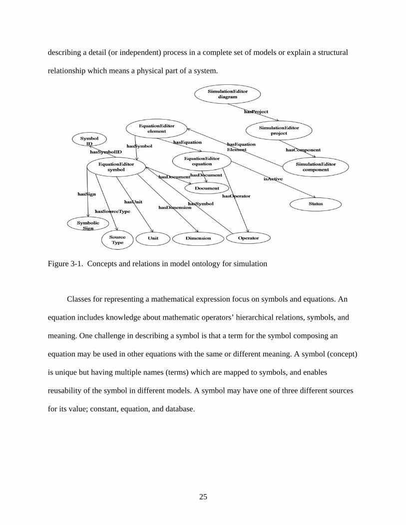
describing a detail (or independent) process in a complete set of models or explain a structural
relationship which means a physical part of a system.
Figure 3-1. Concepts and relations in model ontology for simulation
Classes for representing a mathematical expression focus on symbols and equations. An
equation includes knowledge about mathematic operators’ hierarchical relations, symbols, and
meaning. One challenge in describing a symbol is that a term for the symbol composing an
equation may be used in other equations with the same or different meaning. A symbol (concept)
is unique but having multiple names (terms) which are mapped to symbols, and enables
reusability of the symbol in different models. A symbol may have one of three different sources
for its value; constant, equation, and database.
25
EquationEditor
The EquationEditor is a tool for creating equations associated with a model, and properly
defining symbols appearing in these equations. It provides a facility for creating, browsing, and
inspecting all equations, symbols, and units appearing in the model. It uses an interface that
resembles other equation editors such as Microsoft Office Equation Editor (Microsoft, 2003) and
MatyType (MathType, 1996), but differs significantly because all the symbols in equations and
equations are represented internally by using ontology objects. This provides a way to represent
the meaning of equations and symbols that is not possible with other equation editors.
Equation Object Model (EOM)
The Equation Object Model (EOM) is an intermediate collection of basic objects that
represents information describing a mathematical expression and communicates with the Lyra
physical storage manage to retrieve and store equations and symbols (Figure 3-2). The main
purpose of EOM is to represent the elements of mathematical expressions. Operators and other
symbols of an equation are objects of the two main classes, MathTemplate and MathPrimitive.
MathTemplate defines a type of operator and a collection of arguments. Character symbols and
numerical symbols are subclasses of MathPrimitive. MathSymbol objects representing a symbol
contain two properties; a linguistic-level property and a programmatic-level property. Symbol (in
multiple terms), symbolID, and definition are linguistic-level properties. Programmatic-level
contains three properties; source, matrixType, and matrixSymbolUsage. A property source
represents the origin of the numerical value of the symbol (equationType, databaseType, or
constant). If the symbol is a matrix, property matrixType gives the matrix dimensions. A flag,
"constant" or "variable", is a value representing matrixSymbolUsage property. The value
"constant" means that the value never changes, whereas "variable" means the value can change.
26
Figure 3-2. Class diagram of Lyra equation object model retrieving instances of model ontology
Components of the EquationEditor
The EquationEditor has three sub-editors, Symbol Editor, Mathematical Statement Editor,
and Unit Editor, to create and maintain symbols, equations and symbol units.
Symbol Editor (Figure 3-3) is an editor for individual symbols appearing in equations and
includes a symbolic expression of a symbol, a quantity of measurement, and a description of the
linguistic and programmatic properties of the symbol. A symbol is implemented as a class in the
ontology, which has a unique meaning within a specific domain. Often, the same symbolic
character (term for the symbol) is used over different domains, but is used in different ways and
has different meaning. Since a symbol has a distinguishing identifier representing a specific
27
concept in the ontology, a use of the same term for different symbols is permitted, and the
domain ontologies can be used to resolve their ambiguous meaning.
Figure 3-3. Features of the symbol editor in the EquationEditor: symbol ID, symbol, unit and description of Cell Crop Evapotranspiration
The value of a symbol is determined by one of three methods: from an equation, from a
database, or from a constant which is directly assigned to the symbol. In the case where the
symbol value is determined by an equation, there must be an equation in the database in which
this symbol appears alone on the left side. To obtain the value from the database, some
constraints may be required in order to locate and query a database to obtain the value (e.g. a
current time and a soil layer number for querying a soil temperature at a specific date), and these
constraints can be specified as a part of the symbol’s properties (Figure 3-4).
Symbols can also be arrays, when a symbol can be used in different discrete intervals in
space and time. For example, soil water content can be expressed in different soil layers which
occur in different soil profiles, characterized by the depth from the soil surface, the soil profile
number and time.
28
Figure 3-4. Database constraints and array dimension description of a symbol
Figure 3-5. Equation ID and equation of Cell Evapotranspiration in the mathematical statement editor
29
The mathematical statement editor is designed to graphically create an equation from
existing symbols and mathematical operator templates (Figure 3-5). An equation is an expression
that has a hierarchical tree data structure composed of symbols and operators. The equal operator
is the root node of the tree structure, containing a single symbol on the left branch of the tree.
The value of the left side symbol is defined by the calculation of the right side terms. Thus the
equation is assumed to be a function which has symbols as arguments. The editor provides an
operator template which can describe specific argument sets. There are eight operator groups
used to compose an equation (Table 3-1).
Table 3-1. List of operators in EquationEditor Operator group Operators Exponential Subscript, double subscript, superscript, exponent, sub and super
maximum, minimum Logic And, or, not Arithmetic Add, subtract, multiply, divide, negation Relation Less than, greater than, less and equal, greater and equal, equal,
equivalent, not equal, not equivalent, less than and less than equal to, less than equal to and less than
Case n-case, matrix
The Unit editor is an interface to create and maintain the unit for a symbol and its
compositions for representing the quantity of measurement of symbols (Figure 3-6). Unit
includes not only the generic collection of global standard unit of metric system (e.g.
international system of unit (SI) and the English unit system), but also domain specific units such
as “cm3 of soil” in soil engineering. It is very important to carefully track the units associated
with symbols, since different models may use the same symbol but having different units. A unit
is not represented by a simple string, but by a composition of symbols (like an equation). The
30
unit can be expressed using a composition of limited operators (multiply, divide, and power
operator) and other units. Thus, basic units such as length and weight can be reused for creating a
composite unit, and this makes it possible to automatically calculate conversion of units from
one form to another (e.g. the English unit to the metric unit).
Figure 3-6. Unit ID, unit and definition of centimeter of water in unit editor
SimulationEditor
The SimulationEditor is used to describe the structure of dynamic systems using graphic
elements such as source, sink, storage, and flow. It adopts concepts from the compartmental
modeling technique (Peart and Curry, 1998) and Forrester notation (Forrester, 1971) which is
widely used in agriculture and natural resource models. However, like the EquationEditor, these
concepts are represented internally using the ontology and stored in the Lyra database. The
SimulationEditor is used for specifying the overall model structure in the form of elements, and
31
incorporates the EquationEditor described in the previous section in order to build equations
associated with each element. The SimulationEditor provides a graphic user interfaces to create
and maintain a simulation system which includes a structure design interface, a simulation
control interface, and a simulation result reporting interface. The SimulationEditor also contains
facilities for automatically generating and running simulations and generating reports.
Figure 3-7. Structure editor showing a compartmental diagram of a soil-water model
The structure editor is the main interface of the SimulationEditor and provides
functionalities which enables modelers to create and maintain a simulation project by designing
the structure of a system, and to interact with the EquationEditor and the simulation controller.
Structural design of a system is a procedure by which a modeler creates physical or
environmental elements and relationships in the system by using graphic elements. For example
(Figure 3-7), a 3-dimensional soil profile system may be designed as a composition of soil cell
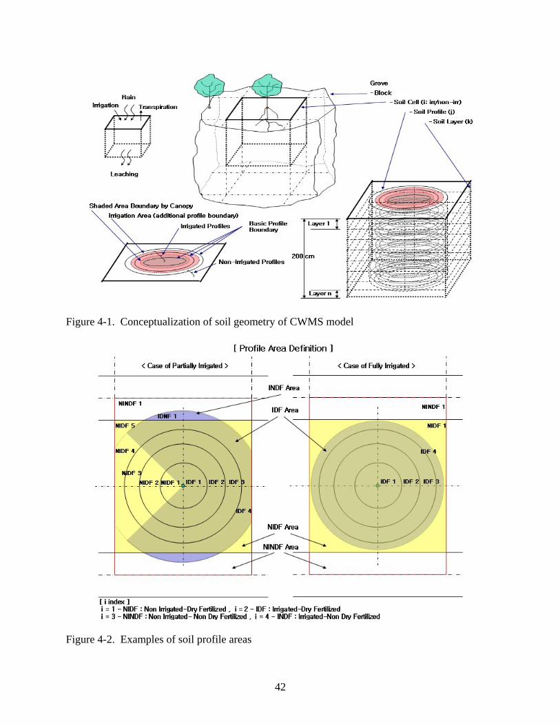
A soil cell consists of a one-tree planting row area with the tree in the center. The width
and length of the cell are in-row and between-row distances to adjacent trees. It includes four-
types of zones (i.e. a non-irrigated & dry-fertilized area, an irrigated & dry-fertilized area, a non-
irrigated & non-dry-fertilized area, and an irrigated and non-dry-fertilized area as shown in
Figure 4-2) according to the irrigation status and the dry-fertilized status, and each zone may
have from 1 to 5 soil profile(s) which consist of n soil layers. The total soil layer number (n) is
determined based on the particular soil type or a depth of each soil layer.
41
Figure 4-1. Conceptualization of soil geometry of CWMS model
Figure 4-2. Examples of soil profile areas
42
Water balance for each profile is determined using rainfall and irrigation events as water
inputs and evapotranspiration (ET) and leaching water as water losses from the balance.
Basically, the water budget calculation is based on the tipping bucket model, enhanced by
considering the effect of the delayed soil water drainage caused by the soil hydraulic
conductivity during one daily time step. It is assumed that water inputs are applied at the first soil
layer. Water infiltration depth is calculated as a function of the infiltration characteristics of the
soil.
A pure tipping bucket model assumes that water moves the entire layer depth in one time
step. Tipping bucket does not always reflect soil water content on a daily time step due to soil
hydraulic characteristics. To account for the hydraulic characteristics of the soil, CWMS assumes
that all irrigation, water with N application and rainfall occurs at noon and has a maximum of 12
hours to move through the soil on the first day. The model calculates the wetting front speed and
the time for which the wetting front travels a layer thickness, thus to obtain the layer index of
wetting front at the end of the day and let unfinished drained water continues to drain at next
day.
As stated above, water loss from the water balance is water drainage below the 200 cm
maximum depth and crop ET. Daily crop ET is calculated in CWMS using reference ET as user
input or from weather data. A crop coefficient based on Morgan et al. (2006b) is applied to the
reference ET based on seasonal variability. The crop ET deducted from each soil profile layer is
proportional to the root length density of the profile layer. A layer root length density distribution
is a function of tree size (Morgan et al., 2006a). An irrigation is scheduled when the CWMS
determines that water content in the irrigated zone is below the allowed depletion. The irrigation
43
duration is determined by the water amount needed to bring water content to field capacity and is
determined by the emitter flow rate, irrigation efficiency, and irrigation depth.
For nutrient management, especially application of nitrogen by irrigation (fertigation), the
CWMS model provides processes for calculating nitrogen balance followed by transformation of
nitrate and ammonium. Transformations are composed of complicated sub-processes and are
affected by input and flow (drainage from above layer) amount of nutrient and water between
layers. The model assumed that there are four nutrient flow processes by four drain events: drain
by rain, pre-irrigation, during-irrigation, and post-irrigation. After four-drain steps,
transformation processes is applied to ammonium and nitrate following in order of volatilization,
uptake of ammonium, uptake of nitrate, and nitrification.
Model Base of the CWMS Model
The CWMS models is implemented by using a taxonomy representing physical
relationship of natural resources (soil profile, crop, and environment), which consists of 4 soil
related concepts (block, soil cell, soil profile, and soil layer), root density, weather, and
irrigation. The system structure taxonomy is built graphically with the SimulationEditor (Figure
3-7).
For the CWMS model approximately 700 symbols and 500 equations were created.
Symbols and equations developed for the CWMS model are interrelated, and their relationship
can be visualized as a graph diagram (Figure 4-3), which displays connections of symbols and
equations used to model the water and nitrogen balance process. Symbols and equations are
represented as rectangular boxes, and the number above a box shows the count of connected
boxes but not displayed. An arrow means that the target symbol is required to calculate the
source equation.
44
Figure 4-3. Relationship among equation symbols for water and nitrogen balance
In the diagram, nitrogen balance process group is connected with the water balance process
group by referencing several equations for water balance. They can be switched with similar
process groups independently. Particular processes, uptake, nitrification and volatilization, are
clustered clearly from other equations in the equation group of nitrogen balance, and for water
balance a similar pattern was found for processes of evapotranspiration, infiltration, and
irrigation. This suggests possibilities for organizing and categorizing models and subprocesses.
45
The graphic in Figure 4-3 is generated automatically from the ontology objects, and an animated
interface allows the model to navigate through the space of symbols.
A model base is a database of many models, model elements, equations, and symbols. It
can be utilized for reusing models by applying a taxonomic organization to an ontology. In
Figure 4-4, a model base is shown, which consists of equations used in the CWMS model. The
taxonomy contains 6 classes including weather, water, nutrient, soil, crop and site. The water
class has 5 subclasses (infiltration, evapotranspiration, precipitation, irrigation and runoff), and
each subclass contains related equations and symbols. For example, the CWMS model includes
two different infiltration models (Tipping Bucket Water Content Equation and Enhanced
Wetting Front Water Content Equation).
Figure 4-4. Taxonomy diagram of the CWMS model
46
Examples of Model Representing Process
Representing a model formed as theoretical or logical expressions (equations) in the
ontology-based simulation system is a process of redefining and adjust them into a real world
simulation for describing a phenomenon. Theoretical models provide the conceptual knowledge,
and there are usually many reformulated models depending on assumptions and the given
situation.
Morgan et al. (2006a) described how they derived the infiltration model used in CWMS
from theoretical models. In summary, their infiltration model is based on Green-Ampt infiltration
(Green and Ampt, 1911) and unsaturated flow based on Richard’s equation (Richards, 1931)
derived from Darcy’s Law for irrigation and rainfall moving into soil from the surface and
moving between soil layers. The Green-Ampt model in the case of no ponding at surface can be
expressed as:
Where,
fp : infiltration capacity of soil (the rate that water will infiltrate as limited by soil factors)
F : cumulative infiltration
Ks : the hydraulic conductivity of the transmission zone
M : the difference between initial and final volumetric water contents
Sf : the effective suction at the wetting front
Furthermore, the model adopted Mein and Larson’s equation (Mein and Larson, 1973)
applying the Green-Ampt model for rainfall conditions by determining cumulative infiltration at
the time of surface ponding. Some assumptions addressing the situation in which the rainfall
47
intensity is less than the infiltration capacity of the soil are focused. The general Mein and
Larson equation can be described as:
Where,
Sav : the average suction at wetting front
Fp : the cumulative infiltration at the time of surface ponding
R : the rainfall intensity
By considering the relation between rainfall intensity, infiltration capacity, and saturated
hydraulic conductivity, the Mein and Larson equation can be written like as:
Morgan et al. assumed that no ponding occurred in the sandy soil (e.g. for Candler soil, Ks
is 25 cm/hour) because rainfall is less than 5 cm/hour (except during hurricanes) and irrigation
rates are typically 0.315 cm/hour or less. It was also assumed that runoff does not exist since the
rainfall and irrigation intensity is usually smaller than Ks. Thus, the infiltration rate equals the
rainfall rate and the amount of infiltration water equals amount of rainfall rate multiplied by time
t. If rainfall rates are larger than the irrigation rate, the infiltration rate equals the rainfall
intensity. Otherwise, it equals irrigation intensity. Thus, the Mein and Larson equation is
simplified for such rainfall and irrigation conditions. The condition term for comparing the rain
48
intensity with the saturated hydraulic conductivity was simplified to comparing the rainfall
amount (represented by PWID4) with the irrigation amount at soil cell (represented by CIAM)
for creating the average infiltration rate of soil profile. To apply the world system to the model,
additional condition term s describing whether current soil profile exists in the irrigated-area or
non-irrigated-area were added to the model. With the above result, an equation for the infiltration
rate of soil profile was formed in Figure 4-5. CIAM is the cell irrigation amount, and i is the
profile type, and numbers (1, 2, 3 and 4) represent the profile type, a non-irrigated & dry-
fertilized area, an irrigated & dry-fertilized area, an irrigated and non-dry-fertilized area, and an
non-irrigated and non-dry-fertilized area. SAKtop is the saturated hydraulic conductivity at
surface, and PWID4 is the soil profile water input amount from rainfall effect. IAM is the
equation calculating irrigation amount from irrigation duration, and IDur is the irrigation
duration time.
Examples of CWMS Model Implementation
Concepts developed above were entered into the ontology system. The geometry relating
soil cell and profile, soil water redistribution, and root density are given below as examples.
Soil geometric dimension
Basically, a profile is determined by the distance from the trunk of a tree to three root zone
radii (75, 125, and 175cm). Other profile boundaries are the irrigation diameter and the dry-
fertilized area. Depending on the irrigation type (360 degree or less than 360 degree), soil
profiles can be divided into irrigated-areas and non-irrigated areas. Irrigation and dry-fertilizing
events are assumed to be conducted in a soil cell area except two equipment drive paths between
tree rows. Therefore, the two drive paths are always considered as a non irrigated & non dry-
fertilized area (NINDF). An irrigated & non-dry fertilized area (INDF) is an irrigated area in the
drive paths.
49
Where,
Figure 4-5. Morgan’s infiltration rate model in the CWMS model
Figure 4-6. Equations of profile number
50
Equations for calculating each profile number and area are defined at the cell, and Figure
4-6 shows equations of three different profile number (profile number of a non irrigated & non
dry-fertilized area is always 1 and it is defined as a constant). NPIDF, NPNIDF, and NPINDF
are respectively symbols of a profile number of an irrigated & dry-fertilized area, a profile
number of a non-irrigated & dry-fertilized area, and a profile number of an irrigated and non-dry-
fertilized area. RZR is a symbol of the root zone radius matrix, and WD is a symbol of the
wetting diameter, and SpP is a symbol of the spray pattern.
A soil layer is one vertical element of a soil profile, and the number of soil layers in a soil
profile is determined by layer thickness and total depth of the soil profile, whose maximum depth
is 200cm. The thickness of soil layers can be grouped, and it is represented as a matrix as in
Figure 4-7. Each row is a layer group, the first column is a thickness of layers in a group, and the
second column is the number of layers in a group, and third column is a cumulative layer number
to that group.
Symbols belonging in concepts, block, soil cell, soil profile, and soil layer, are required
dimensions. The time dimension is a common dimension required by most symbols as one
dimension of the matrix. Symbols in block and soil cell need only the time dimension, whereas
those in soil profile need three dimensions, one for time, one for soil profile type, and one for
soil profile number. Symbols in the soil layer need four dimensions, and they include three
dimensions from soil profile and one for soil layer number. For example, a symbol, historical soil
layer temperature, defined in soil layer has four dimensions, and it is described through the
EquationEditor (Figure 4-8).
51
Figure 4-7. Layer thickness matrix
Figure 4-8. Example of dimension description of a symbol in soil layer
Time step
The main time step for the model is daily. Rain event, irrigation event, and fertilizer
applications are assumed to occur at 12:00 pm, but adjustments to the time period of 0-12:00 pm
and 12:00 pm - 24:00 pm are controlled by using some time flag symbols. The minimum period
of simulation which can be executable is 14 days. The first 13 days (for 14 days calculation) or
first 5 years (for 20 years calculation) are used to initialize and stabilize values of symbols whose
initial condition are not known at the simulation starting time. For example, the initial values of
soil water content is usually unknown, but assumed to be a default value and computed over the
13 days (or 5 years) to initialize the values.
52
Figure 4-9. Total number of time steps symbol, t
There are two concepts related with time. One is Total Number of Time Steps for
assigning system time dimension size, a value that is stored in and obtained from the database
(Figure 4-9). The other concept related with time is Index variable of Time Step, t, which is used
as the general variable for the current time.
Root density
As shown in Figure 4-10, root density is represented as a matrix from the model for each
soil depth and root sections based on root density distribution as a function of tree size (Morgan
et al., 2006a). A column is a root section and a row is a soil layers group to a specific depth.
Following Morgan’s model, the root horizontal area is divided into four sections (0-75 cm, 75-
125 cm, 125-175cm and 175cm-boundary), and 10 soil layer groups are used. The first 6 rows
have thicknesses 15 cm and last 4 rows have 30 cm thicknesses, which are calculated by
proportional equations based on the root density value of 6th soil depth group. RD is a symbol of
53
the root density, and cv is a symbol of the canopy volume, and RSL is a matrix symbol of the
root density regression parameters for layers below 6th soil depth group.
The root density equation is designed for specific soil layer depths and root ranges. The
CWMS model utilizes it for an equation of LRD which is the layer root density (Figure 4-11).
LD and LT are symbols of the layer depth and thickness of a layer at specific depths.
Figure 4-10. Root density matrix
54
Figure 4-11. Layer root density equation
Water dynamics
The water balance model consists of rainfall, irrigation, evapotranspiration, and infiltration.
As stated previously, surface runoff and subsurface lateral flow are not considered due to the
high saturated hydraulic conductivity of sandy soils. Basically, the water budget calculation is
based on the tipping bucket model, enhanced by considering the effect of the delayed soil water
drainage which is caused by the soil hydraulic conductivity during one daily time step.
Rainfall and irrigation are water inputs into the system, and it is assumed that they are
applied at the first layer. The symbol Profile Water Input (PWI) in the soil profile module
represents input water amount from water resources into the soil profile. According to the
CWMS model, it considers the complicated nutrient management processes by calculating
different sources of water and nutrient separately. In the equation for PWI, sources of water
inputs are distinguished as 4 different types depending on the considering event: irrigation
(water), N application, post N application, and rainfall. Since the system time step is daily and
55
there is no sub-time step, symbols are created for every stage and distinguished by subscript
number. These are four-drain process named. Figure 4-12a shows related PWI equations (PWI1,
PWI2, PWI3, and PWI4), where it is assumed that irrigation and N application are applied to just
irrigated-area (i=2).
The symbol WI (Figure 4-12b) is the layer water input, and the amount is determined by
the difference of amount of input water into a layer from environment (PWI) or from the upper
layer (DW) and the amount of layer evapotranspiration (nowET). For the four-drain process,
calculation of layer water input is conducted for every stage separately. The symbol WIflag is for
indicating the status of the remained water drain by the hydraulic conductivity.
A layer water content is represented by the symbol WC whose amount is calculated by the
difference of increasing amount (WCpos) by drained water and decreasing amount (WCneg) by
evapotranspiration during the previous time step. At the start of simulation all layer water
content has same amount calculated with constant depletion level. For the four-drain process, a
layer water content at time t would be a WCD4 of previous time step which is the layer water
content applying irrigation, N application, post N application, and rainfall (Figure 4-12c).
The CWMS model enhanced the pure tipping bucket model by computing the wetting front
moving speed during the simulation, whereas the pure tipping bucket model assumed that water
moves the entire layer depth in one time step. The model assumed that all irrigation, water with
N application, water with post N application and rainfall occurs at noon and has a maximum of
12 hours to move through the soil on the first day after irrigation, water with N application, water
with post N application or rainfall. And, the model calculates the wetting front speed (Figure 4-
13) and the time for which the wetting front travels a layer thickness, thus to obtain the layer
index of wetting front at the end of the day and let unfinished drained water continues to drain at
56
next day. WFSP is the layer wetting front speed, and it can be calculated by the symbol of the
infiltration WFSP (Figure 4-13b) or the symbol of the hydraulic conductivity WFSP (Figure 4-
13c). Figure 4-13d is the equation for hydraulic conductivity.
A
B
C
Figure 4-12. Water balance equations: A) profile water input amount equations, B) layer water input amount equation, and C) layer water content equation
57
A
B
C
D
Figure 4-13. Enhanced hydraulic conductivity related equations in CWMS model: A) Wetting front speed equation, B) infiltration wetting front speed equation, C) hydraulic conductivity wetting front speed equation, and D) hydraulic conductivity equation
Nitrogen balance
For nutrient management, especially application of nitrogen by irrigation (fertigation), the
CWMS model provides processes for calculating nitrogen balance followed by transformation of
nitrate and ammonium. Transformations are composed of complicated sub-processes and are
affected by input and flow (drain from above layer) amount of nutrient and water between layers.
The model assumed that there are four nutrient flow processes by four drain events: drain by
rain, pre-irrigation, during-irrigation, and post-irrigation. After four-drain steps, transformation
processes is applied to ammonium and nitrate following in order of volatilization, uptake of
ammonium, uptake of nitrate, and nitrification.
The amount of nitrogen input into a soil profile is an equation formed with the dissolved
ammonium (NH4) and nitrate (NO3) nitrogen amount of dry fertilizer by rain or irrigation and
58
fertilizer amount during the fertigation. Nitrogen drain amounts (ammonium and nitrate) of a
layer from the above layer are represented by symbols, Layer Drained Nitrate and Layer Drained
Ammonium, and they are calculated by equations of soluableRate. For uptake amounts of
nitrogen, passive uptake of ammonium and active/passive uptake of nitrate are formed as an
equation. Also, the model assumed that the uptake process of ammonium occurred after
volatilization and nitrification follows a nitrate uptake process, and they are utilized by using
separate symbols for each stage.
The amount of nitrification is represented by symbol NIT, and its equation includes the
rate of maximum nitrification as a function of ammonium content (NH4NC3), maximum
nitrification amount at a time (NITVmax), half-saturation constant of nitrification (NITkm), and
soil moisture factor (NITwf). Nitrification is allowed till 80% of current ammonium content
Volatilization (cumulativeVOLA) is created at the soil profile module, since volatilization
occurs till 5cm soil depth from the surface. It represents a cumulative volatilization loses over a
day, which is determined by the relationships between ammonium content (VolPNH4NIn), days
counting from the volatilization starting time (NApplyElapse), percentage of maximum
cumulative volatilization (qm), and site-specific temperature/wind parameters (Figure 4-15).
Application Implementation
The CWMS model is used to implement a CWMS application program for use by grower
that utilizes crop, soil and weather data. A CWMS application consists of the automatically
generated simulation code and a graphic user interface. The generated simulation code is plugged
into the graphic user interface without further coding required.
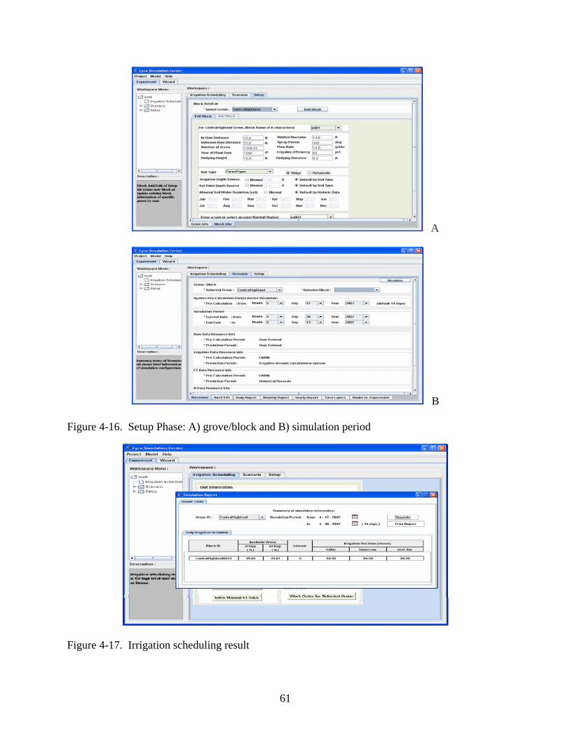
A graphic user interface allows growers to interact with the system through three phases:
the setup, the irrigation scheduling, and reporting. The setup phase is for configuring the cell and
block information for a particular grove (Figure 4-16a) and for describing simulation site,
start/end data, and resource location (Figure 4-16b). The simulation period is separated into an
initializing period and a simulation period. For a long term simulation, an initializing period can
be longer than 14 days which is the default initializing period for farm irrigation scheduling.
The irrigation scheduling phase, shown in Figure 4-17 provides irrigation scheduling
information to growers. By default, it is based on a 14-day simulation followed by a 3-day
prediction period (the simulation period can be extended) to provide immediate term
recommendations on irrigation rates. In order to plan a strategy on irrigation scheduling,
simulation system tested for full seasons (over 250 days per year and over 30 years).
60
A
B
Figure 4-16. Setup Phase: A) grove/block and B) simulation period
Figure 4-17. Irrigation scheduling result
61
A
B
Figure 4-18. Simulation results: A) table and B) graph
62
Detailed simulation results are provided in the form of daily, monthly, and yearly reports
(Figure 4-18). The daily report contains each layer’s root length, water content, nitrate and
ammonium content, and soil coefficient. Data can be browsed by selecting a specific date and
profile type. The monthly report shows data for a particular month including irrigation interval
days and duration, evapotranspiration, crop coefficient, soil coefficient, water and nutrient
leaching amount at 2 m depth and irrigation depth, rain, and irrigation. The yearly report
provides the monthly total value of irrigation, rain, water and nutrient leaching amount at 2 m
depth and irrigation depth, and fertilizing amount. Water, nitrate, and ammonium content
contained in the daily report can be displayed as a chart.
Model Extension
The CWMS Java code was generated automatically by the SimulationEditor and the
EquationEditor, and can be used as a software component that can be used independently of the
model building environment. The compiled Java code can be easily connected to other user
interfaces or simulation system. For example, the Watershed Assessment Model (WAM) which
is used as a part of a larger FDACS BMP simulation, adopted the CWMS model as a sub-
component of land use in citrus production. The CWMS model provides information about
leached water and nutrient amounts to the host simulation system.
A key issue was how easily the CWMS model could be modified for integration with
WAM. A water and nitrogen balance model needed by the WAM was required to use several
new soil types, and modifications to the model were made to support these new parameters.
Using the EquationEditor, new symbols for soil types and parameters were created and existing
equations were modified by replacing old symbol and by adding new formula, and some new
equations calculating required values by the WAM were added into the model. This was all
63
accomplished with less than 10 hours of work including creation of required file input/output
protocol by WAM (that took about 80% of total work hours).
Model Performance
Simulation of the CWMS model containing approximately 700 symbols and 500 equations
uses different numbers of equations depending on the combination of processes (e.g. use process
of tipping bucket or effect of hydraulic conductivity). To test the performance of the CWMS
model for the maximum number of processes, the combination including hydraulic conductivity,
four-drain process and moving wetting front is chosen, which consists of 330 equations.
Applying dimension size to these equations, total number of calculation at double precision level
is 330,000 for 14 days period. It takes approximately 5 seconds by a computer with Intel Pentium
1.7GHz CPU speed and 1G RAM. Calculation time for 1, 10 and 30 years are 24 seconds, 5
minutes and 15 minutes, respectively. For an extension for WAM which contains process of
tipping bucket and moving wet front, it takes 5 minutes for 30 years simulation. In order to
validate the accuracy of the model, Morgan (Morgan et al., 2006a) compared the observed water
contents at soil depth 10, 20, 30 and 50cm from foil surface with 2 years simulation result for
two different sites. According to the validation result, R2 values were varied in the range
between 0.46 and 0.75, and for soil depth 10 and 20 cm it gave 0.7 R2 average value which is
higher than another two points. The validity of the model depends on the accuracy of the
equations and parameters, and is impacted by the quality of the model implementation platform.
Model Sensitivity Analysis
Sensitivity analysis is useful method to guide model development as well as to understand
model behavior when the model is under construction. This method is applied to the CWMS
model for identifying most significant factors to Cell Water Amount (CWA) and determining
their interaction, which has been implemented at the SimulationEditor as an additional feature.
64
The procedure consists of two steps: a factor screening with Morris randomized OAT design and
a global sensitivity analysis with screened factors.
At the factor screening step, a variable (e.g. CWA, a sum of water amount in the soil cell)
is selected to analyze the response of the system to the CWMS models’ water balance processes.
Variables related with the tree characteristics, water inputs (rain and irrigation) and water
movement are selected as an input factor (Table 4-1).
Table 4-1. Input factors related with water input and hydraulic conductivity no Symbol ID Symbol min max unit 1 Canopy Volume cv 3.2 12.6 m2 2 Emitter Flow Rate EFR 20 70 L/hr 3 Hydraulic Conductivity Parameter n HCPn 2.6 4.6 - 4 Initial Depletion Dini 0.09 0.19 - 5 Irrigation efficiency IE 79 89 % 6 Readily Available Coefficient KRA 0.03 0.13 - 7 Wetted Diameter WD 100 500 cm
The selected variable used for tree characteristic was canopy volume (CV, volume of a
citrus tree as function of tree age). Selected water input variables were emitter flow rate (EFR,
the volume of water discharged from the emitter within a period of time), initial depletion (Dini,
the initial condition of depletion), and irrigation efficiency (IE, the percentage of water pumped
into the irrigation system that actually gets distributed by the emitter) and wetted diameter (WD,
the diameter of the irrigation emitter). The selected variables for water movement were soil
hydraulic conductivity (HCPn), was assumed to same for all soil layers, and readily available
coefficient (KRA, coefficient used to calculate the readily available water content for uptake for
uptake).
The minimum and maximum values of factors six different variables in Table 4-1 were
applied. Six orientation matrices are generated according to the Morris factor-screening design,
and the respective elementary effects for 7 different factors per orientation matrix are estimated
65
from the simulation response for CWA. Following Morris OAT design 8 simulation
configurations are generated for each of six orientation matrices. In each orientation matrix, the
first row represents the base case (configuration) and the remaining 7 are used to determine the
elementary effects for all 7 factors involved.
After comparing the elementary effects of 7 factors for 6 different trajectories and the
corresponding mean and variance of the distribution, factor 7, the WD, appears significantly
separated from the other factors and it means that the wetted diameter dominate the simulation
result. The WD increases value of CWA since it determine direct water input amount from
irrigation event, but its effect compared with other factors was explained before this analysis.
Whereas, factor 5 and 6, IE and KRA, has lower mean-variance relation value than other factors,
so that model results are less sensitive those two factors were screened before sensitivity analysis.
At the sensitivity analysis step, 35 complete factorial design makes 243 scenarios with the
5 factors selected by the Morris OAT screening-factor method and 3 different factor levels. The
analysis of variance on the simulation result of CWA was performed, which included
interactions between two different factors. The results presented in Table 4-2 shows the sum of
squares and the sensitivity index which is calculated by dividing the sum of squares with the total
variability.
From the result of sensitivity analysis, the CWA was apparently governed by the WD, and
Dini with a significant impact on the system than other factors. The HCPn was more sensitive
than the CV and the EFR. The EFR appeared as the least sensitive factor among the main factors.
The WD related the water input to the amount of irrigation. Thus, water balance could be
affected significantly by the irrigation amount when there was less rainfall. For the interaction
between two factors, the interaction of the WD and the CV was more significant than others, and
66
interactions with the HCPn had relatively larger value than other interactions because it
contributed to increase water amount in deep soil layer. The CV affected rainfall into the system
by blocking direct rain, and limited amount of rain could reach to soil.
Table 4-2. Sensitivity analysis result including main effects and two-factor interactions Effects SS
Sensitivity analysis result provides information about impact factors and related factors
impacts. It may be useful to reconfigure model parameter and to create other models using these
symbols.
In Chapter 4, the CWMS model developed by Morgan et al. (Morgan et al., 2006a; Morgan
et al., 2006b) is implemented using ontology-based simulation methodologies and tools covered
in Chapter 3. Soil geometry structure is designed with 4 concepts, soil block, soil cell, soil profile,
and soil layer and their dimensions are defined with index concepts describing array size. With
the existing mathematical models symbols and equations are defined and entered into the
ontology, and they formed a model base containing symbols and equations and structuring
relation between them. Model performance is tested under two different simulation conditions,
and using a sensitive analysis tool, critical input factors and the associated factor relations are
revealed for water amount in the soil system. Through these processes the CWMS model is
created and executed efficiently by the graphic interface program.
67
CHAPTER 5 SUMMARY AND FUTURE WORK
The following methodologies were developed utilizing ontology-based simulation
techniques to build mathematical models.
1) The EquationEditor includes a symbol dictionary for entering symbols appearing in
the equations along with their definitions and units. Symbols are defined by
specific concepts. Equation are rendered visually using classic mathematical
notation, but internally a hierarchical data structure (tree) is used for storing
operators and symbols. The equal operator is the root node of the equation tree.
Operators (like + and -) used in the equation become a node in the tree with child
nodes being additional operators or symbols. The Equation Object Model (EOM)
used in the Equation Editor is a collection of basic objects which represent
information describing a mathematical expression and defining data type of
attributes, and which communicate with ontology-based database system to retrieve
data.
2) The SimulationEditor incorporates the EquationEditor and is designed to represent
the structure of dynamic systems using graphic elements. The SimulationEditor
also contains facilities for automatically generating and running simulations and
providing reports. The SimulationEditor provides a graphic user interface to create
and maintain a simulation system; a structure design interface for the simulation
system, a simulation control interface, a simulation result reporting interface, and
some additional interfaces including a math markup language generator and a
statistical model analyzer.
68
These methodologies were applied to develop a model of the Citrus Water Management
System. Approximately 700 symbols and 500 equations are conceptualized and stored in
ontology database using the SimulationEditor and EquationEditor. A Java program for running
the simulation was generated automatically from the modeling environment and incorporated
into both a stand-alone application for grower and WAM. The modeling environment provides
adequate tools to create and modify models without any programming knowledge. From the
results, it can be concluded that ontology-based simulation offers a significant improvement in
the methodology for building, publishing, and managing model.
For the next step, it will be useful to study model reusability within the existing model base
of the CWMS model. Issues on model reusability are related with the scale of models in the
problem domain, which requires the consistency of the temporal and spatial scale to guaranty
compatibility in models (Leon et al., 2002). For a similar scale domain problem with the CWMS
model, such as models using different soil profiles, limitation placed on reusing these sub-
models are that they have rigid and sophisticate connections with other processes such as a
hydraulic conductivity which has strict requirement for spatial scale. On the other hand, from an
extension study of the CWMS model, WAM, in which two different models cooperate
independently keeping the internal scale of the model may cause significant inefficiency of
simulation time. There are needs for an efficient way to organize and classify models and
processes within a model base and for a flexible way to constructing a set of simulation model
for different project and modeler by switching with a different process. Diverse level taxonomic
categories may help the model base to be handled more intuitively.
The data reusability could follow the model reusability. Especially, relational databases are
important sources of data for simulation model, but it is expensive to identify existing data, to
69
determine the exact format of data and to use data in a model. There has been research to convert
directly relational databases directly to ontology using a mapping language (Barrasa et al., 2004)
and to transform/service various heterogeneous database sources including database as
ontologies (TopBraid, 2003). It is difficult to provide a formal way to use databases as ontologies
since security and restriction level of data varies and case depends on the domain. Therefore, it
will be useful to study sharing databases as a form of ontology for a simulation model in the
agriculture domain to build an efficient simulation model network. This study can include
methods to publish/search databases, negotiate/communicate automatically to get wanted data,
and provide a protocol for networking within the domain. Finally, a visual environment will be
required to enhance the reusability of models and data and ontology since they have a
complicated relationship and structure. There are some studies on solving complexity problem
in displaying ontology visually (Bosca et al., 2005; TouchGraph, 2005), but it needs to develop
methods focusing on the relations in model and data.
70
LIST OF REFERENCES
Alam, F. M. and K. R. McNaught, 2004, Using Morris’s Randomized OAT Design as Factor Screening Method for Developing Simulation Metamodels, Proc. Of the 2004 Winter Sim. Conf. Vol. 1:930-938 Athanasiadis, I. N., A. E. Rizzoli, M. Donatelli and L. Carlini, 2006, Enriching software model interfaces using onotlogy-based tools, iEMSs, Burlington, Vermont, July 2006 Ausbrooks, R., S. Buswell and D. Carlisle, 2003, Mathematical Markup Language (MathML) Version 2.0, http://www.w3.org/TR/MathML Barrasa, J., O. Corcho and A. G´omez-P´erez, 2004, R2O, an Extensible and Semantically Based Database-to-ontology Mapping Language, Second Workshop on Semantic Web and Databases (SWDB2004). Toronto, Canada. August 2004 Beck, H. W., 2007, Lyra ontology management system, http://orb.at.ufl.edu/ObjectEditor/index.html Beck, H. W., L. G. Albrigo and S. Kim, 2004, DISC citrus planning and scheduling program, Proceeding of the Seventh International Symposium on Modelling in Fruit Research and Orchard Management: 25-32 Benjamin, P. C., M. Patki and R. J. Mayer, 2006, Using ontologies for simulation modeling, Winter Simulation Conference 2006: 1151-1159 Booch, G., J. Rumbaugh and I. Jacobson, 1997, The Unified Modeling Language user guide, Addson-Wesley Bosca, A., D. Bonino and P. Pellegrino, 2005, OntoSphere: more than 3D ontology visualization tool, SWAP 2005, the 2nd Italian Semantic Web Workshop, Trento, Italy, December 14-16, 2005, CEUR Workshop Proceedings Buswell, S., O. Caprotti, D. P. Carlisle, M. C. Dewar, M. Gaetano and M. Kohlhase, 2004, The OpenMath Standard 2.0, http://www.openmath.org/standard/om20-2004-06-30/ Cuske, C., T. Dickopp and S. Seedorf, 2005, JOntoRisk: An Ontology-based Platform for Knowledge-based Simulation Modeling in Financial Risk Management, European Simulation and Modeling Conference 2005 Donatelli, M., G. Bellocchi and L. Carlini, 2006a, Sharing knowledge via software components: models on reference evapotranspiration, Europ. J. Agronomy Vol. 24(2): 186-192 Donatelli, M., G. Bellocchi and L. Carlini, 2006b, A software component for estimating solar radiation, Environmental Modelling and Software Vol. 21(3): 411-416
Eitzinger, J., M. Trnka, J. Hosch, Z. Zalud and M. Dubrovsky, 2004, Comparison of CERES, WOFOST and SWAP models in simulating soil water content during growing season under different soil conditions, Ecological Modelling Vol. 171(3): 223-246 Ewert, F., H. Van Keulen, M. K. Van Ittersum, K. E. Giller, P. A. Leffelaar and R. P. Roetter, 2006, Multi-scale analysis and modelling of natural resource management, Proceedings of the iEMSs, Burlington, Vermont, July 2006 Fishwick, P. A. and J. A. Miller, 2004, Ontologies for Modeling and Simulation: Issues and Approaches, Proceeding of 2004 Winter Simulation Conference, Vol. 1:251-256 Forrester, J. W., 1971, World Dynamics, Cambridge, MA: Productivity Press: 144 Furmento, N., A. Mayer, S. McGough, S. Newhouse, T. Field and J. Darlington, 2001, Optimisation of component-based applications within a grid environment, Proceedings of the 2001 ACM/IEEE conference on Supercomputing, Denver, CO, November 2001 Green, W. H. and G. Ampt, 1911, Studies of soil physics, part 1.-the flow of air and water through soils, J. Agricultural Science Vol. 4: 1-24 Gruber, T. R., 1995, Toward Principles for the Design of Ontologies Used in Knowledge Sharing, International Journal of Human Computer Studies Vol. 45:907-928 Guarino, N., 1997, Understanding, building and using ontologies, Int. J. Human-Computer Studies Vol.46, 293-310 Haan, C. T., H. P. Johnson and D. L. Brakensiek, 1982, Hydrologic modeling of small watersheds, ASAE Monograph No. 5:533 Islam, A. S. and M. Piasecki, 2004, A Stategy for Web-Based Modeling of Hydrodynamic Processes, EM2004 June 13-16 Ittersum, M. K. v., F. Ewert, T. Heckelei, J. Wery, J. Alkan Olsson, E. Andersen, I. Bezlepkina, F. Brouwer, M. Donatelli, G. Flichman, L. Olsson, A. E. Rizzoli, T. van der Wal, J. E. Wien and J. Wolf, 2008, Integrated assessment of agricultural systems - A component-based framework for the European Union (SEAMLESS), Agricultural Systems, Vol. 96(1-3):150-165 Jones, J. W., B. A. Keating and C. H. Porter, 2001, Approaches to modular model development, Agricultural Systems 70: 421-443 Jurisica, I., J. Mylopoulos and E. Yu, 2004, Ontologies for Knowledge Management: An Information Systems Perspective, Knowledge and Information Systems Vol. 6: 380-401 Knublauch, H., D. Oberle, P. Tetlow and E. Wallace, 2006, A Semantic Web Primer for Object-Oriented Software Developers, W3C Working Group Note 9 March 2006
72
Lacy, L. and W. Gerber, 2004, Potential modeling and simulation applications of the web ontology language - OWL. WSC '04: Proceedings of the 36th conference on Winter simulation, Winter. Leon, L. F., D. Lam, S. Hamilton, N. Crookshank, D. Bonin and D. Swayne, 2002, Multi-model integration in decision support system: a technical user interface approach for watershed and lake management scenarios, Proceeding of 2002 iEMSs Vol. 3: 306 Lu, H.-Y., C.-T. Lu, M.-L. Wei and L.-F. Chan, 2004, Comparison of Different Models for Nondestructive Leaf Area Estimation in Taro, Agron J Vol. 96(2): 448-453 MathType, 1996, Design Science, http://www.dessci.com/en/products/mathtype/ Mein, R. G. and C. L. Larson, 1973, Modeling infiltration during a steady rain, Water Resour. Res. Vol. 9(2): 384-394 Microsoft, 2003, Microsoft Office Equation Editor, http://office.microsoft.com/en-us/word/HP051902471033.aspx Miller, J. A., G. T. Baramidze, A. P. Sheth and P. A. Fishwick, 2004, Investigating ontologies for simulation modeling. Simulation Symposium, 2004. Proceedings. 37th Annual. Morgan, K. T., T. A. Obreza and J. M. S. Scholberg, 2006a, Characterizing citrus tree root distribution in space and time, J. Am. Soc. Hort. Sci. Vol. 131: 149-156 Morgan, K. T., T. A. Obreza, J. M. S. Scholberg, L. R. Parsons and T. A. Wheaton, 2006b, Citrus water uptake dynamics on a sandy Florida Entisol, Soil Sci. Soc. Am. J. Vol. 70(1): 90-97 Morris, M. D., 1991, Factorial Sampling Plans for Preliminary Computational Experiments, Technometrics Vol. 32(2) Muetzelfeldt, R. and J. Massheder, 2003, The Simile visual modelling environment, Europ. J. Agronomy Vol. 18: 345 Noy, N. F. and D. L. McGuinness, 2001, Technical Report KSL_01_05, Ontology Development 101: A Guide to Creating Your First Ontology, Stanford Knowledge Systems Laboratory Park, M. and P. A. Fishwick, 2005, Integrating Dynamic and Geometry Model Components through Ontology-Based Interface, Simulation Vol. 81(12): 795-813 Peart, R. M. and R. B. Curry, 1998. Agricultural systems modeling and simulation. New York, Marcel Dekker. Raubel, M. and W. Kuhn, 2004, Ontology-based task simulation, Spatial Cognition and Computation Vol. 4: 15-37
Reddy, V. and V. Anbumozhi, 2004, DEVELOPOMENT AND APPLICATION OF CROP SIMULATION MODELS FOR SUSTAINABLE NATURAL RESOURCE MANAGEMENT, International Agricultural Engineering Conference (IAEC) Richards, L. A., 1931, Capillary conduction through porous mediums, Physics Vol. 1: 313-318 Rizzoli, A. E., M. Donatelli, R. Muetzelfeldt, T. Otjens, M. G. E. Sevensson, F. v. Evert, F. Villa and J. Bolte, 2004, SEAMFRAME, A Proposal for an Integrated Modelling Framework for Agricultural Systems, Proc. of the 8th ESA Congress: 331-332 Rumbaugh, J., M. Blaha, W. Premerlani, F. Eddy and W. Lorensen, 1991, Object-oriented modeling and design, Englewood Cliffs, New Jersy: Prentice Hall Scholten, H., A. Kassahun, J. C. Refsgaard, T. Kargas, C. Gavardinas and A. J. M. Beulens, 2007, A methodology to support multidisciplinary model-based water management, Environmental Modelling & Software Vol. 22(5): 743-759 Steed, M., 1992, Stella, a simulation construction kit: cognitive process and educational implications, The Journal of Computers in Mathematics and Science Teaching Vol. 11(1): 39 TopBraid, 2003, TopQuadrant White Paper, http://www.topquadrant.com TouchGraph, 2005, TouchGraph White Paper, http://www.touchgraph.com/ Wallach, D., D. Makowski and J. W. Jones, 2007, Working with Dynamic Crop Models, Elsevier