ONTROL OPTIM c - Courant Institute of Mathematical …stadler/papers/HerzogStadlerWach...S u−y d 2...

Copyright © by SIAM. Unauthorized reproduction of this article is prohibited.

SIAM J. CONTROL OPTIM. c© 2012 Society for Industrial and Applied MathematicsVol. 50, No. 2, pp. 943–963

DIRECTIONAL SPARSITY IN OPTIMAL CONTROL OF PARTIALDIFFERENTIAL EQUATIONS∗

ROLAND HERZOG† , GEORG STADLER‡ , AND GERD WACHSMUTH†

Abstract. We study optimal control problems in which controls with certain sparsity patternsare preferred. For time-dependent problems the approach can be used to find locations for control de-vices that allow controlling the system in an optimal way over the entire time interval. The approachuses a nondifferentiable cost functional to implement the sparsity requirements; additionally, boundconstraints for the optimal controls can be included. We study the resulting problem in appropriatefunction spaces and present two solution methods of Newton type, based on different formulations ofthe optimality system. Using elliptic and parabolic test problems we research the sparsity propertiesof the optimal controls and analyze the behavior of the proposed solution algorithms.

Key words. sparsity, optimal control, control device placement, L1-norm minimization, semi-smooth Newton

AMS subject classifications. 49K20, 65K10, 49M15, 49J52

DOI. 10.1137/100815037

1. Introduction. Optimal control problems with control costs of L1-type areknown to produce sparse solutions [8, 26], i.e., the control function is identically zeroon parts of the domain. Since at these points no control needs to be applied, problemswith sparsity terms naturally lend themselves to situations where the placement ofcontrol devices or actuators is not a priori given but is part of the problem.

In this paper, we analyze a general class of optimal control problems with asparsity measure that promotes striped sparsity patterns. As a model problem inL2(Ω), we consider

(P1)Minimize J(u) =

1

2‖Su− yd‖2H +

α

2‖u‖2L2(Ω) + β ‖u‖1,2

subject to ua ≤ u ≤ ub a.e. in Ω,

where H is a Hilbert space corresponding to the state space of the controlled system,yd ∈ H is the desired state, and S : L2(Ω) → H is the linear control-to-state mapping.Moreover, −∞ ≤ ua < 0 < ub ≤ ∞ are bound constraints for the optimal controls,α ≥ 0, β > 0, and ‖u‖1,2, which as specified below favors sparse solutions. To motivatethe approach, in this introduction we assume that Ω = Ω1 × (0, T ) is a space-timecylinder, where Ω1 ⊂ R

n, n ≥ 1, and T > 0, in which case the directional sparsityterm is given by

(1.1) ‖u‖1,2 :=∫Ω1

(∫ T

0

u2 dt

)1/2

dx.

∗Received by the editors November 15, 2010; accepted for publication (in revised form) November2, 2011; published electronically April 19, 2012.

http://www.siam.org/journals/sicon/50-2/81503.html†Faculty of Mathematics, Chemnitz University of Technology, D–09107 Chemnitz, Germany

([email protected], [email protected]).‡Institute for Computational Engineering & Sciences, University of Texas at Austin, Austin, TX

78712 ([email protected]). The work of this author was partly supported by National ScienceFoundation grant CCF-0427985.

943


944 ROLAND HERZOG, GEORG STADLER, AND GERD WACHSMUTH

This term measures the L1-norm in space of the L2-norm in time. We will show thatthe term ‖u‖1,2 leads to certain, in applications often desirable, sparsity patterns forthe optimal controls u. We refer to (P1) as problem with a directional sparsity term.

To explain our interest in (P1), consider a modified problem (P0), in which ‖u‖1,2is replaced by

(1.2) ‖u‖0,2 := μ(C) with C :=

{x ∈ Ω1 :

∫ T

0

u2 dt > 0

}⊂ Ω1,

where μ denotes the Lebesgue measure. The term ‖u‖0,2 accounts for costs originatingfrom the sheer possibility to apply controls at certain locations. For example, thiscould be acquisition costs for control devices or actuators, in which case β is the priceper control device unit. At a solution of (P0), C is the set where placing controldevices is most efficient. Terms such as (1.2) are also called “L0-quasi-norms” sincethey can be found as (formal) limits of Lp-quasi-norms as p → 0. Unfortunately, usingthe sparsity term (1.2) results in a nonconvex, highly nonlinear, and to some extentcombinatorial problem since the set C depends on the (unknown) solution.

However, the directional sparsity problem (P1) can be used as a convex relaxationof the L0-problem. Partial theoretical justification for this approximation can, for in-stance, be found in [4, 11, 12]. We point out that using the “undirected” sparsity termβ ‖u‖L1(Ω) also results in a solution with a certain sparsity structure. However, thissparsity pattern changes over time. Compared to solutions based on the directionalsparsity terms ‖u‖0,2 or ‖u‖1,2, where the sparsity structure is fixed over time, this isdifficult to realize in practice.

Besides the practical relevance of (P1) for finding optimal locations for controldevices, studying (P1) is also of theoretical interest. Since the functional (1.1) cannotbe differentiated in a classical sense, subdifferentials have to be used and the con-struction of efficient solution algorithms becomes challenging. Even though choosingα > 0 (which we mostly assume in this paper) allows us to formulate the problemin a Hilbert space framework, the problem structure and the characteristics of thesolution are very different from smooth optimal control problems.

Let us put our work into perspective. Nonsmooth terms in optimization prob-lems with PDEs are commonly being used for the purpose of regularization in in-verse problems in image processing; see, for instance, [6, 23, 24, 30]. Among thefew papers where L1-regularization is used in the context of optimal control of PDEsare [5, 8, 26, 31, 32]. In [5, 8, 26, 32] elliptic optimal control problems with the non-directional sparsity terms β ‖u‖L1(Ω) are analyzed. In [5, 26, 32], in additional to thesparsity term, the squared L2-norm α/2 ‖u‖2L2(Ω) is part of the cost functional, whichallows the problem to be analyzed and solved by a Newton-type algorithm in a Hilbertspace framework. On the contrary, in [8] the problem is posed and analyzed in L1(Ω)or BV(Ω) and a Newton-type algorithm is proposed that applies to a regularized ver-sion of the problem. In [32], convergence rates as α → 0 are investigated. Comparedto [8, 26, 32], in the problem (P1) under consideration here, points in the controlspace are directionally coupled, which leads to a stronger nonlinearity in the opti-mality system. Additional challenges arise from the combination of pointwise boundconstraints with the nonlocal sparsity term. In [31], the authors use L1-regularizationfor a system of ODEs, which is driven toward a desired state at final time. Here,the nonsmooth objective is motivated by the physics of the problem (the control costmeasures the consumption of fuel) rather than by the need for sparse optimal con-trols. Related research focuses on finding sparse solutions to finite-dimensional, linear


DIRECTIONAL SPARSITY IN OPTIMAL CONTROL OF PDEs 945

x1

x2

Ω2(x

1)

x1Ω1

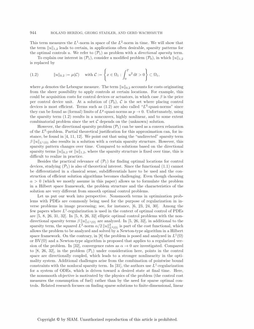
Fig. 1.1. Two-dimensional example domain Ω, its projection Ω1, and the cross section Ω2(x1).

inverse problems. For underdetermined problems, the convex relaxed l1-norm prob-lem provably finds a near-optimal solution also with respect to l0, i.e., the sparsestsolution [4, 11, 12]; we refer to [29] for an overview of numerical methods employed inthis context. In a different interpretation of the sparsity approach, the authors in [15]find optimal experimental designs for linear inverse problems. Here, a sparsity termis used to rule out experiments that do not contribute significant information for theinversion. In practice, this can reduce the number of experiments or measurementsto be made.

The main focus of this paper is twofold. First, we analyze (P1) in a functionspace framework, derive the optimality system, and study characteristics of the sparseoptimal controls. Second, we propose two Newton-type algorithms for the numericalsolution of (P1) and study their convergence behavior. To the authors’ knowledge,available algorithms for finite-dimensional counterparts of (P1) are based only onfirst-order information; see, for example, [22, 25, 34].

The outline of the remainder of this paper is as follows. In section 2, we provethe existence and uniqueness of a solution for (P1) and derive necessary and sufficientoptimality conditions. In section 3, we present a particular form of the optimalitysystem that applies in the absence of pointwise control constraints. Local superlinearconvergence of a semismooth Newton method based on this form is proved. Section 4is devoted to an alternative formulation of the optimality system, which allows tak-ing into account pointwise control constraints. We also derive a semismooth Newtonmethod based on this formulation and study its properties in finite dimensions. Fi-nally, in section 5 properties of solutions of (P1) are studied using numerical examples,and the efficiency of the algorithms proposed in this paper is analyzed.

Notation. While a time-dependent problem has been used in the introductionfor illustration purposes, in the remainder of this paper we allow for a more generalsplit of coordinate directions, which contains the time-dependent problem as a specialcase (see Example 1.2). Throughout the paper, Ω ⊂ R

N with N ≥ 2 is a boundedmeasurable set. The coordinate directions are partitioned according to R

N = Rn ×

RN−n for some 1 ≤ n < N . This induces the sets

Ω1 = {x1 ∈ Rn : ∃x2 ∈ R

N−n with (x1, x2) ∈ Ω},(1.3a)

Ω2(x1) = {x2 ∈ RN−n : (x1, x2) ∈ Ω} for x1 ∈ Ω1.(1.3b)

Hence, Ω1 can be interpreted as the projection of Ω onto Rn, whereas Ω2(x1) is the

cross section of Ω at position x1 ∈ Rn (see Figure 1.1). The general form for the



directional sparsity term ‖u‖1,2 is

(1.4) ‖u‖1,2 :=∫Ω1

(∫Ω2(x1)

u2(x1, x2) dx2

)1/2

dx1.

We now give two examples of problems that fit into our general framework.Example 1.1 (elliptic PDE). The domain Ω ⊂ R

N is a bounded domain withLipschitz boundary, and S : L2(Ω) → H := L2(Ω) denotes the solution map u → y ofthe elliptic PDE

−Δy = u in Ω, y = 0 on Γ.

Example 1.2 (parabolic PDE). This is a particular case of the example describedin the introduction. Suppose that Ω1 ⊂ R

n is a bounded domain with Lipschitzboundary Γ, Ω2 = (0, T ) for some T > 0, and Ω = Ω1×Ω2 is the space-time cylinder.Moreover, for κ > 0, S : L2(Ω) → H := L2(Ω) denotes the solution operator u → yfor

yt −∇ · (κ∇)y = u in Ω, y = 0 on Γ× (0, T ), y(·, 0) = 0 in Ω1.

In both examples, the restriction to homogeneous boundary and initial data canbe waived by modifying yd. Note that problems with vector-valued control variablesu : Ω → R

n, or equivalently u : Ω × {1, 2, . . . , n} → R, are included in our settingif the inner integral in (1.4) is taken with respect to the counting measure. Theregularization term then becomes ‖u‖1,2 :=

∫Ω‖u(x)‖Rn dx, where ‖·‖Rn denotes the

Euclidean norm in Rn. Problems of this type fall into the class of joint sparsity

approaches; see [13, 14].

Function spaces. We denote by Lp(Ω), Lp(Ω1), and Lp(Ω2(x1)) the classicalLebesgue spaces on the respective domains (1 ≤ p ≤ ∞). The norm in these spacesis referred to as ‖·‖p, and the domain will be clear from the context. We write 〈· , ·〉for the scalar product in L2. For 1 ≤ p, q ≤ ∞, we denote by Lp,q(Ω) the space of(equivalence classes of) all measurable functions f : Ω → R whose norm

‖f‖p,q :=∥∥Ω1 � x1 → ‖f(x1, ·)‖q

∥∥p

is finite. In case Ω2(x1) does not depend on x1, this is the usual Bochner spaceLp(Ω1, L

q(Ω2)). In the general case, it is a closed subspace of the latter with Ω2 =∪x1∈Ω1Ω2(x1) being the union of all cross sections. Nevertheless, we also refer toLp,q(Ω) as a Bochner-type space. Finally, for functions u, v defined on Ω we introducethe shorthand notation

|u|x1,2 :=

(∫Ω2(x1)

u2(x1, x2) dx2

)1/2

= ‖u(x1, ·)‖2,

〈u, v〉x1,2 :=

∫Ω2(x1)

u(x1, x2) · v(x1, x2) dx2 = 〈u(x1, ·), v(x1, ·)〉.

That is, | · |x1,2 is the L2-norm and 〈· , ·〉x1,2 the scalar product on the stripe {x1} ×Ω2(x1). Note that for u, v ∈ L2(Ω), the relations |u|·,2 ∈ L2(Ω1) as well as 〈u, v〉·,2 ∈L1(Ω1) hold.

Standing assumptions. We consider problem (P1) under the following assump-tions. H is a Hilbert space, and yd ∈ H is the desired state. We assume that



S ∈ L(L2(Ω), H) is a bounded linear map. For the analysis of the semismooth New-ton method in section 3, we require

(1.5) S�S : L2(Ω) → L6,2(Ω) to be bounded, and S�yd ∈ L6,2(Ω).

Here, we denoted by S� the adjoint of S. Moreover, let ua, ub ∈ L2(Ω) and denote by

(1.6) Uad := {u ∈ L2(Ω) : ua ≤ u ≤ ub a.e. in Ω}the set of admissible controls. It is reasonable to suppose that ua < 0 < ub holds a.e.in Ω, which makes u ≡ 0 an admissible control. Finally, we assume α ≥ 0, β > 0.

Note that (1.5) is satisfied for the examples mentioned above in reasonable di-mensions. First we consider Example 1.1 with N ≤ 3. Due to the smoothing propertyof the control-to-state mapping, S� maps L2(Ω) continuously into H1

0 (Ω). Sobolev’sembedding theorem ensures H1

0 (Ω) ↪→ L6(Ω), and by Holder’s inequality we can inferL6(Ω) ↪→ L6,2(Ω). Altogether, S� maps L2(Ω) continuously into L6,2(Ω). Let us nowconsider Example 1.2 with n ≤ 3. The solution theory for parabolic equations yieldsthe continuity of S� : L2(Ω) → L2(0, T ;H1

0(Ω1)). By Sobolev’s embedding theoremwe have L2(0, T ;H1

0(Ω1)) ↪→ L2(0, T ;L6(Ω1)). For functions f ∈ L2(0, T ;L6(Ω1))the continuous Minkowski inequality (see [9, p. 499]) yields f ∈ L6(Ω1;L

2(0, T )) andmoreover

‖f‖L6(Ω1;L2(0,T )) ≤ ‖f‖L2(0,T ;L6(Ω1)).

Therefore, we have L2(0, T ;L6(Ω1)) ↪→ L6(Ω1;L2(0, T )) = L6,2(Ω). Altogether we

infer the continuity of S� : L2(Ω) → L6,2(Ω).

2. Analysis of the problem. In this section, we prove the existence anduniqueness of an optimal solution for (P1) and derive necessary and sufficient op-timality conditions. We begin by computing the subdifferential of ‖u‖1,2.

2.1. Computation of the subdifferential. Due to the separability of L2(Ω2)we can use a standard result [10, p. 282] to find the dual of the Bochner-type spaceL1,2(Ω). A direct proof can be found in [33, Satz 3.11].

Lemma 2.1. The dual space of L1,2(Ω) can be identified with the Bochner-typespace L∞,2(Ω). This is the space (of equivalence classes) of all measurable functionsϕ defined on Ω whose norm

‖ϕ‖∞,2 := ess supx1∈Ω1

(∫Ω2(x1)

ϕ2(x1, x2) dx2

)1/2

is finite. The dual pairing is given by

〈u, ϕ〉L1,2(Ω),L∞,2(Ω) =

∫Ω

u · ϕ d(x1, x2).

Lemma 2.2. The subdifferential of ‖·‖1,2 : L1,2(Ω) → R at u ∈ L1,2(Ω) is givenby

(2.1) ∂‖·‖1,2(u) = {v ∈ L∞,2(Ω) : v(x1, ·) ∈ ∂‖·‖2(u(x1, ·)) for all x1 ∈ Ω1}with the subdifferential of the L2(Ω2(x1))-norm

s ∈ ∂‖·‖2(w) ⇔{‖s‖2 ≤ 1 if w = 0 a.e. on Ω2(x1),

s = w‖w‖2

elsewhere,



where w ∈ L2(Ω2(x1)). An equivalent characterization of the subdifferential of ‖·‖1,2is given by

v ∈ ∂‖·‖1,2(u) ⇔ for a.a. x1 ∈ Ω1 :

{|v|x1,2 ≤ 1 if |u|x1,2 = 0,

v(x1, ·) = u(x1,·)|u|x1,2

if |u|x1,2 �= 0.

The subdifferential remains the same if ‖·‖1,2 is considered a function of L2(Ω) → R.Proof. We begin by observing that (see [20, p. 56])

(2.2) ∂‖·‖1,2(u) = {v ∈ L∞,2(Ω) : ‖v‖∞,2 ≤ 1, 〈u, v〉L1,2(Ω),L∞,2(Ω) = ‖u‖1,2}.To show that the right-hand sides in (2.2) and (2.1) coincide, let v ∈ ∂‖·‖1,2(u)be given. The first condition in (2.2) yields |v|x1,2 ≤ 1 for almost all x1 ∈ Ω1.Furthermore, we have

‖u‖1,2 =∫Ω1

∫Ω2(x1)

u · v dx2︸︷︷︸=:f(x1)

dx1.

Now, for almost all x1 ∈ Ω1 it holds that f(x1) = 〈u, v〉x1,2 ≤ |u|x1,2|v|x1,2 ≤ |u|x1,2.Therefore, we have

‖u‖1,2 =∫Ω1

f(x1) dx1 ≤∫Ω1

|u|x1,2 dx2 = ‖u‖1,2.

Together, these relations imply that f(x1) = |u|x1,2 holds for almost all x1 ∈ Ω1. This,in turn, shows v(x1, ·) ∈ ∂‖·‖2(u(x1, ·)). The converse inclusion can be proved easily.

If ‖·‖1,2 is considered as a function from L2(Ω) into R, the subdifferential maybecome larger. However, it remains a subset of L∞,2(Ω), and thus the density of L2(Ω)in L1,2(Ω) shows that the subdifferentials coincide. Indeed, suppose vk → v in L1,2(Ω)with vk ∈ L2(Ω). Let g be a subgradient (w.r.t. L2(Ω)) of ‖·‖1,2 at u ∈ L2(Ω), i.e.,

‖w‖1,2 ≥ ‖u‖1,2 + 〈g, w − u〉 for all w ∈ L2(Ω).

Using w = vk and passing to the limit shows the same inequality with w replaced byv ∈ L1,2(Ω).

2.2. Existence, uniqueness, and optimality conditions.Lemma 2.3. Problem (P1) has a unique solution for β ≥ 0 and α > 0. The same

holds for α = 0 in case S is injective.Proof. For α > 0 the objective J(u) is strictly convex and continuous. The

same holds true in case α = 0, provided that S is injective. Furthermore, theset Uad ⊂ L2(Ω) is convex and weakly compact and therefore the existence anduniqueness of the optimal control follows from standard arguments; see, for instance,[28, Thm. 2.14].

The variational inequality

(2.3) 〈u− u, ∂J(u)〉 ≥ 0 for all u ∈ Uad

is a necessary and sufficient optimality condition for (P1). Hence the Moreau–Rocka-fellar theorem [20, p. 57] implies the following lemma.

Lemma 2.4. The function u ∈ L2(Ω) solves (P1) if and only if

(2.4) 〈u − u, −p+ βλ+ αu〉 ≥ 0

holds for all u ∈ Uad, where p = S�(yd − Su) is the adjoint state and λ ∈ ∂‖·‖1,2(u)is a subgradient as defined in (2.1).



With the introduction of a Lagrange multiplier μ associated with the conditionu ∈ Uad, the variational inequality (2.4) becomes

(2.5a) −p+ βλ+ αu + μ = 0,

where λ and μ satisfy

(2.5b) λ ∈ ∂‖·‖1,2(u), μ(x1, x2)

⎧⎪⎨⎪⎩≤ 0 if u(x1, x2) = ua(x1, x2),

≥ 0 if u(x1, x2) = ub (x1, x2),

= 0 else

in an almost everywhere sense. Sections 3 and 4 present two different formulations ofthis optimality system, which lead to different solution algorithms.

3. Semismooth Newton method I: The unconstrained case. SemismoothNewton methods are well studied in both finite-dimensional and function spaces, andthey are commonly used for optimal control problems; see [2, 16, 21]. Under certainconditions, a local superlinear convergence rate and even global convergence can beproved. The aim of this section is to present a semismooth Newton method for thecase that no bound constraints for the controls are present in (P1), i.e., Uad = L2(Ω).For this case we can show local superlinear convergence of the method in functionspace. To this end we state an alternative form of the optimality system (2.5) that istailored to the unconstrained case. In this section, α > 0 is assumed throughout.

Lemma 3.1. In the case Uad = L2(Ω), u ∈ L2(Ω) is the optimal solution of (P1)if and only if

(3.1) u = max

(0, 1− β

|p|·,2

)p

αa.e. in Ω

holds, where p = S�(yd − Su) is the adjoint state.Proof. Let us show the equivalence of (3.1) and (2.5). Note that Uad = L2(Ω)

implies μ = 0 and let x1 ∈ Ω1 be given. If |u|x1,2 = 0, both systems are equivalent to|p|x1,2 ≤ β. Suppose now that |u|x1,2 > 0. Then both systems imply that u(x1, ·) is amultiple of p(x1, ·). Now we have the equivalences

(2.5) ⇔ p(x1, ·) = (α+ β |u|−1x1,2

)u(x1, ·) ⇔ |p|x1,2 = α |u|x1,2 + β

⇔ |p|x1,2 − β = α |u|x1,2 ⇔ (3.1),

which shows the equivalence.This lemma gives rise to the definition of the nonlinear operator F : L2(Ω) →

L2(Ω)

F (u) := u−max

(0, 1− β

|Pu|·,2

)Pu

α,

where Pu := S�(yd−Su) is the adjoint state belonging to u. As a direct consequenceof Lemma 3.1, we have that F (u) = 0 if and only if u solves (P1).

In the remainder of this section we prove the Newton (or slant) differentiability[7, 16] of F and the invertibility of the derivative F ′(u).

Lemma 3.2. The function G : L6,2(Ω) → L2(Ω) defined by

p → max

(0, 1− β

|p|·,2

)p



is Newton differentiable on L6,2(Ω) and a generalized derivative is given by

G′(p)h = max

(0, 1− β

|p|·,2

)h+ χp

β 〈h, p〉·,2|p|3·,2

p with χp =

{1 if |p|·,2 > β,

0 else.

Proof. Let p, h ∈ L6,2(Ω) be given. We define the remainder r(h) by

r(h) = G(p+ h)−G(p)−G′(p+ h)h

=

[max

(0, 1− β

|p+ h|·,2

)−max

(0, 1− β

|p|·,2

)− χp+h

β 〈h, p+ h〉·,2|p+ h|3·,2

]p

−[χp+h

β 〈h, p+ h〉·,2|p+ h|3·,2

]h

= (r1 + r2 + r3) p− r4 h,

where

r1 = χN1

(1− β

|p+ h|·,2 −(1− β

|p|·,2

)− β

〈h, p+ h〉·,2|p+ h|3·,2

),

r3 = χN3

(1− β

|p|·,2

),

r2 = χN2

(1− β

|p+ h|·,2 − β〈h, p+ h〉·,2|p+ h|3·,2

),

r4 = χp+hβ 〈h, p+ h〉·,2

|p+ h|3·,2

with

N1 := {x ∈ Ω : |p+ h|·,2 > β, |p|·,2 ≥ β},N2 := {x ∈ Ω : |p+ h|·,2 > β, |p|·,2 < β},N3 := {x ∈ Ω : |p+ h|·,2 ≤ β, |p|·,2 > β}.

Now we estimate the four parts of the sum for r(h) separately.First part. On N1 we have

r1 = β

(− 1

|p+ h|·,2 +1

|p|·,2 − 〈h, p+ h〉·,2|p+ h|3·,2

)

=β

|p+ h|3·,2 |p|·,2(|p+ h|2·,2

(|p+ h|·,2 − |p|·,2)− |p|·,2 〈h, p+ h〉·,2

)≤ β

|p+ h|3·,2 |p|·,2(|p+ h|·,2 〈h, p+ h〉·,2 − |p|·,2 〈h, p+ h〉·,2

)by Cauchy–Schwarz

=β

|p+ h|3·,2 |p|·,2(|p+ h|·,2 − |p|·,2

)〈h, p+ h〉·,2 ≤ β

|p+ h|2·,2 |p|·,2|h|2·,2 ≤ |h|2·,2

β2.



Similarly, we obtain the lower bound

r1 =β

|p+ h|3·,2 |p|·,2(|p+ h|2·,2

(|p+ h|·,2 − |p|·,2)− |p|·,2 〈h, p+ h〉·,2

)≥ β

|p+ h|3·,2 |p|·,2

(|p+ h|2·,2|p|·,2 〈p, h〉·,2 − |p|·,2 〈h, p+ h〉·,2

)by Cauchy–Schwarz

=β

|p+ h|3·,2 |p|2·,2((|p+ h|2·,2 − |p|2·,2

) 〈p, h〉·,2 − |p|2·,2 |h|2·,2)

=β

|p+ h|3·,2 |p|2·,2((

2 〈p, h〉·,2 + |h|2·,2) 〈p, h〉·,2 − |p|2·,2 |h|2·,2

)≥ −β

|p+ h|3·,2 |p|2·,2(|p|2·,2 |h|2·,2 + |h|3·,2 |p|·,2

)≥ −|h|2·,2

β2− |h|3·,2

β |p|·,2 .

This implies ‖p r1‖2L2(Ω) ≤ 2 β−4 (‖p‖2L6,2(Ω) ‖h‖4L6,2(Ω) + β2‖h‖6L6,2(Ω)).

Second part. On N2 we have

0 ≤ 1− β

|p+ h|·,2 =|p+ h|·,2 − β

|p+ h|·,2 ≤ |h|·,2β

and β|〈h, p+ h〉·,2||p+ h|3·,2

≤ |h|·,2β

,

and hence |r2| ≤ 2 β−1 |h|·,2. Due to β > |p|·,2 > β − |h|·,2 we have μ(N2) → 0 as‖h‖ → 0. This implies ‖p r2‖2L2(Ω) ≤ 4 β−2 ‖p‖2L6,2(Ω) ‖h‖2L6,2(Ω) ‖χN2‖2L6,2(Ω).

Third part. On N3 we have

0 ≤ r3 = 1− β

|p|·,2 =|p|·,2 − β

|p|·,2 ≤ |h|·,2|p|·,2 ≤ |h|·,2

β.

Due to β < |p|·,2 ≤ β + |h|·,2 we have μ(N3) → 0 as ‖h‖ → 0. This implies‖p r3‖2L2(Ω) ≤ β−2 ‖p‖2L6,2(Ω) ‖h‖2L6,2(Ω) ‖χN3‖2L6,2(Ω).

Fourth part. We have

|r4| = χp+h

∣∣∣∣∣β 〈h, p+ h〉·,2|p+ h|3·,2

∣∣∣∣∣ ≤ β−1 |h|·,2.

This implies ‖h r4‖2L2(Ω) ≤ β−2 ‖h‖4L4,2(Ω).Combining the estimates. Due to the above estimates we obtain

‖r(h)‖L2(Ω) ≤ ‖p r1‖L2(Ω) + ‖p r2‖L2(Ω) + ‖p r3‖L2(Ω) + ‖h r4‖L2(Ω)

= o (‖h‖L6,2(Ω)) as ‖h‖L6,2(Ω) → 0,

which proves that G is Newton differentiable with G′ as a derivative.Due to F = I − α−1G ◦ P and the assumption (1.5) that the affine operator P

maps L2(Ω) continuously to L6,2(Ω), we obtain the Newton differentiability of F .Corollary 3.3. The function F : L2(Ω) → L2(Ω) is Newton differentiable and

a generalized derivative is given by

F ′(u) = I +1

α(G′ ◦ P )(u) ◦ S�S.

This corollary shows that F ′(u) is the sum of the identity operator and the com-position of two operators. To show the bounded invertibility of F ′(u), we investigate



its spectrum. To this end, we cite the following lemma from [18, Prop. 1] and derive acorollary. Recall that an operator A on a Hilbert space is called positive if 〈Av, v〉 ≥ 0holds for all v.

Lemma 3.4. Let A and B be operators on a Hilbert space, let B be positive, anddenote by

√B the positive square root of B. Then

σ(AB) = σ(BA) = σ(√BA

√B).

Corollary 3.5. Let A and B both be positive operators on a Hilbert space withone of them self-adjoint. Then σ(AB) ⊂ [0,∞).

Proof. We first assume that B is self-adjoint. Therefore,√B is self-adjoint

as well. This implies that√BA

√B = (

√B)�A

√B is positive, and thus σ(AB) =

σ(√BA

√B) ⊂ [0,∞). The result for self-adjoint A follows analogously.

We shall apply this corollary to infer the invertibility of F ′(u), using the settings

(3.2) A = G′(P (u)), B = S�S,

both considered as operators from L2(Ω) into itself. Clearly, B is positive and self-adjoint. The positivity of A is shown as part of the proof of the following lemma.

Lemma 3.6. For every u ∈ L2(Ω), the bounded linear mapping F ′(u) : L2(Ω) →L2(Ω) is invertible and ‖F ′(u)−1‖ ≤ 1 holds.

Proof. In order to get a better understanding of the structure of F ′(u) we definefor p = Pu the linear maps

χ : L2(Ω) → L2(Ω), (χv)(x1, ·) ={0 if |p|x1,2 < β,

v(x1, ·) otherwise,

Q : L2(Ω) → L2(Ω), (Qv)(x1, ·) ={0 if |p|x1,2 < β,

β |p|−1x1,2

v(x1, ·) otherwise,

R : L2(Ω) → L2(Ω), (Rv)(x1, ·) ={0 if |p|x1,2 < β,

p(x1, ·) |p|−2x1,2

〈v, p〉x1,2 otherwise.

Note that R is the L2(Ω)-orthogonal projector onto the subspace spanned by thestripes of p, i.e., onto the subspace{

u ∈ L2(Ω) : ∃μ ∈ L2(Ω1) : u(x1, ·) = 0 if |p|x1,2 < β

and u(x1, ·) = μ(x1) |p|−1x1,2

p(x1, ·)}.

With these definitions we have

A = G′(P (u)) = χ−Q+QR.

In order to prove the invertibility of F ′(u) we perform two steps.First step. We show that A is a positive operator. Since R is a projector, I−R is

a projector as well. In particular, this implies ‖R− I‖ ≤ 1. Due to ‖Q‖ ≤ 1 we have‖QR − Q‖ ≤ 1. Therefore I + QR − Q is positive. Using χQ = Qχ = Q, Rχ = R,and the self-adjointness of χ, we see that χ+QR−Q = χ (I +QR−Q)χ is positiveas well.

Second step. We apply Corollary 3.5 to infer the invertibility of F ′(u) and thebound for F ′(u)−1. Applying Corollary 3.5 with the setting (3.2) yields σ(G′(P (u)) ◦



S�S) ⊂ [0,∞). By Corollary 3.3 we infer σ(F ′(u)) ⊂ [1,∞). This implies the invert-ibility of F ′(u) as well as ‖F ′(u)−1‖ ≤ 1 independent of u ∈ L2(Ω).

Using classical arguments (see, e.g., [7, Thm. 3.4]) the Newton differentiability ofF and the uniform boundedness of F ′(u)−1 imply the following result.

Theorem 3.7. The semismooth Newton method

uk+1 = uk − F ′(uk)−1F (uk)

converges locally to the unique solution of (3.1) with a superlinear convergence rate.We remark that it is possible to include in (3.1) constraints of the form

(3.3) |u|·,2 ≤ ub,

where ub ∈ L1(Ω1). This constraint bounds the norm of u on each stripe. For thatcase, the optimality system (3.1) has to be replaced by

(3.4) u = min

(ub, max

(0,

|p|·,2 − β

α

))p

|p|·,2 .

The Newton differentiability and the bounded invertibility of the generalized deriva-tive of (3.4) can be shown as for the unconstrained case. We also mention that con-straints of the type (3.3) are the weakest constraints which ensure the solvability of(P1) without additional L

2-regularization, i.e., for α = 0: note that the solution spaceL1,2(Ω) is not reflexive, but the set of admissible controls satisfying (3.3) is weaklycompact, and the existence of a solution in L1,2(Ω) follows by standard arguments.The inclusion of pointwise control bounds into an optimality system of the form (3.1)is not possible because the additional pointwise complementarity conditions interferewith the stripewise structure of (3.1).

4. Semismooth Newton method II: The constrained case. In this section,we propose an alternative approach to solving (P1), which is based on a differentreformulation of the optimality conditions. This form allows for the incorporation ofpointwise bound constraints since it uses u and λ, while (3.1) is a reduced form thatinvolves only the adjoint state. While being more flexible, a drawback of the approachin this section is that it only applies to the discretized, finite-dimensional problem andpermits only a limited analysis. Since the finite-dimensional min- and max-functionsused in the reformulation are semismooth [7, 16], we can compute a slant derivative.However, the resulting semismooth Newton iteration is well defined only under certainconditions (see Lemma 4.2). In numerical practice, we modify the semismooth Newtonstep to enforce these conditions and observe that these modifications are necessaryonly in the initial steps of the iteration. The equivalent form for the optimality systemis given next.

Lemma 4.1. The function u ∈ L2(Ω) solves (P1) if and only if there existλ, μ ∈ L2(Ω) such that the following equations are satisfied a.e. in Ω:

−p+ βλ + αu+ μ = 0,(4.1a)

max(1, |λ+ c1 u|·,2) λ− (λ+ c1 u) = 0,(4.1b)

μ−max(0, μ+ c2 (u− ub))−min(0, μ+ c2 (u− ua)) = 0,(4.1c)

where c1, c2 > 0 are arbitrary and p = S�(yd − Su).Proof. The reformulation of optimality conditions originating from pointwise

control constraints using complementarity functions is well known (see, e.g., [16, 21,



26]). Thus, we skip the proof of the equivalence between (4.1c) and (2.5) and restrictourselves to showing the equivalence between (4.1b) and λ ∈ ∂‖·‖1,2(u), the lattermeaning |λ|·,2 ≤ 1 and

λ = u/|u|·,2 on {x ∈ Ω : |λ|·,2 = 1},(4.2a)

u = 0 on {x ∈ Ω : |λ|·,2 < 1}.(4.2b)

First, we show that (4.2) implies (4.1b). We first consider the case x1 ∈ Ω1 with|λ + c1 u|x1,2 ≥ 1, and thus we are necessarily in case (4.2a). Hence, max(1, |λ +c1 u|x1,2) λ− (λ + c1 u) = (|u|−1

x1,2+ c1)u − (|u|−1

x1,2+ c1)u = 0. If, on the other hand,

|λ+c1 u|x1,2 < 1, then we are necessarily in case (4.2b) and (4.1b) follows immediatelyfrom u = 0.

Conversely, let us assume that (4.1b) holds. We first study x1 ∈ Ω1 with |λ +c1 u|x1,2 ≥ 1, in which case (4.1b) implies that |λ|x1,2 = 1 and that λ = α u for some α.Plugging this expression for λ into (4.1b) shows that α = |u|−1

x1,2, yielding (4.2a). If on

the other hand |λ+ c1 u|x1,2 < 1, we obtain from (4.1b) that u = 0 on {x1}×Ω2(x1),and thus also |λ|x1,2 < 1, resulting in (4.2b).

The form (4.1) of the optimality conditions motivates the application of a New-ton algorithm as in section 3. A formal computation of a semismooth Newton stepfor u, p, λ, and μ in (4.1) results in the following Newton iteration: Given currentiterates (uk, pk, μk, λk), compute the new iterates (uk+1, pk+1, μk+1, λk+1) by solvingthe system

pk+1 − S�(yd − Suk+1) = 0 on Ω,(4.3a)

−pk+1 + β λk+1 + αuk+1 + μk+1 = 0 on Ω,(4.3b)

uk+1 = 0 on Bk,(4.3c) (I −Mk

)λk+1 − c1M

kuk+1 = F k (λk + c1 uk) on Ck := Ω \ Bk,(4.3d)

uk+1 = ua on Aka,(4.3e)

uk+1 = ub on Akb ,(4.3f)

μk+1 = 0 on Ω \ (Aka ∪ Ak

b ).(4.3g)

Above,

(4.3h)

Bk = {(x1, x2) ∈ Ω : |λk + c1 uk|x1,2 ≤ 1},

Aka = {x ∈ Ω : μk + c2 (u

k − ua) < 0},Ak

b = {x ∈ Ω : μk + c2 (uk − ub) > 0},

I denotes the identity, and the linear operators F k,Mk are given by

F k : v(x1, x2) → 〈γk, v〉x1,2|γk|−1x1,2

λk(x1, x2),(4.4)

Mk : v(x1, x2) → |γk|−1x1,2

(v(x1, x2)− F kv(x1, x2)

),

where γk := λk + c1 uk. Next, we study various aspects of (4.3), which motivate

modifications that lead to an inexact semismooth Newton method that convergesglobally in numerical practice. First, we restrict ourselves to the case without controlconstraints, which amounts to μ = 0 in (4.1a) and omits (4.1c). We also assume thatthe problem has been discretized by finite differences or nodal finite elements in a way



that preserves the splitting of RN into Rn and R

N−n. The discrete approximationor coefficient vectors are denoted with the subscript “h.” For simplicity, we assumethat these vectors are of size N = N1N2, where N1 and N2 correspond to a tensorialdiscretization of the Ω1 and the Ω2(x1) direction, respectively. The individual nodesof Ω1 are denoted by xj

1 and we follow a discretize-then-optimize approach. The

matrix Sh ∈ RN×N is the discretization of the operator S. For a vector vh ∈ R

N , wedenote by vhj ∈ R

N2 the components of vh corresponding to {xj1}×Ω2(x

j1), such that

〈vh, wh〉j := v�hjNhjwhj ∈ R

corresponds to the discretization of the inner product 〈·, ·〉x1,2. Here, Nhj ∈ RN2×N2

is the symmetric mass matrix for the Ω2(x1) direction, and the overall L2-mass matrix

Nh ∈ RN×N acts on vectors uh, wh by w�

h Nhuh =∑N1

j=1 nj w�hjNhjuhj with weights

nj > 0. The mass matrix in H is denoted by Lh ∈ RN×N . Note that for a finite

difference approximation, these mass matrices are diagonal. The norm correspondingto 〈·, ·〉j is defined by |vh|j :=

√〈vh, vh〉j . Then, with ph = S�h (yd,h − Shuh) we

obtain the discrete optimality condition

S�h LhShuh + βNhλh + αNhuh − S�

h Lhyd,h = 0,(4.5a)

max(1, |λh + c1 uh|j)λhj − (λhj + c1 uhj) = 0 for j = 1, . . . , N1.(4.5b)

Note thatNhλh ∈ ∂(∑N1

j=1 nj(u�hjNjuhj)

1/2) holds. Computing a semismooth Newton

step (see [16, 27]) for uh, λh in (4.5) results in the following iteration: Given ukh, λ

kh,

compute the new iterates uk+1h , λk+1

h by solving

−S�h Lh(yd,h − Shu

k+1h ) + βNhλ

k+1h + αNhu

k+1h = 0,(4.6a)

uk+1hj

= 0 for j ∈ Bkh,(4.6b) (

Ihj −Mkhj

)λk+1hj

− c1Mkhjuk+1hj

= gkhjfor j ∈ Ck

h(4.6c)

with Bkh = {j : |λk

h + c1 ukh|j ≤ 1 for j = 1, . . . , N1}, Ck

h := {1, . . . , N1} \ Bkh, and

F khj

=1

|γkh |j

λkhj(γk

hj)�Nhj ,(4.7a)

Mkhj

=1

|γkh |j(Ihj − F k

hj

),(4.7b)

gkhj=

1

|γkh |j

F khjγkhj

= λkhj,(4.7c)

where γkh := λk

h + c1 ukh. We observe that (4.6) are the discretized form of (4.3b)–

(4.3d) for μk+1 = 0 and after elimination of pk+1 using (4.3a). The following resultconcerns the existence of a solution for the discrete Newton step (4.6).

Lemma 4.2. We set c1 := αβ−1. Provided that for all j ∈ Ckh holds |λk

h|j ≤ 1and that

(4.8) 〈γkh , λ

kh〉j > max

(0, |γk

h|j |λkh|j − 2 |γk

h|2j + 2 |γkh|j),

the linear system (4.6) admits a unique solution.



Proof. A straightforward computation shows that for j ∈ Ckh,

(Ihj −Mkhj)−1 =

|γkh |j

|γkh |j − 1

(Ihj −

1

|γkh |2j − |γk

h |j + 〈γkh , λ

kh〉j

λkhj(γk

hj)�Nhj

).

Since |γkh |j > 1 and 〈γk

h, λkh〉j ≥ 0, the matrix (Ihj − Mk

hj)−1 is well defined. From

(4.6c) follows

λk+1hj

= αβ−1((Ihj −Mk

hj)−1 − Ih

)uk+1hj

+ (Ihj −Mkhj)−1gkhj

,

where the fact that (Ihj −Mkhj)−1Mk

hj= (Ihj −Mk

hj)−1 − Ih is used. Plugging this

expression for λk+1hj

into (4.6a) yields

(4.9) S�h LhShu

k+1h + α

∑j∈Ck

h

njNhj(Ihj −Mkhj)−1uk+1

hj= gkh

with gkh := S�h Lhyd,h − β

∑j∈Ck

hnjNhj (Ihj − Mk

hj)−1gkhj

. Since S�h LHSh is positive

semidefinite, it is sufficient to show that the matrix Nhj (Ihj − Mkhj)−1 is positive

definite. For that purpose, we choose a discrete vector uh with uhi = 0 for i ∈ Bkh

and a j ∈ Ckh and obtain

u�hjNhj((Ihj −Mk

hj)−1uhj =

|γkh|j

|γkh |j − 1

(|uh|2j −

〈uh, λkh〉j〈uh, γ

kh〉j

|γkh|2j − |γk

h|j + 〈γkh , λ

kh〉j

)

≥ |γkh|j

|γkh |j − 1

⎛⎝|uh|2j −|uh|2j

(〈γkh , λ

kh〉j + |λk

h|j |γkh|j)

2(|γk

h |2j − |γkh|j + γk

hλkhj

)⎞⎠

=|uh|2j |γk

h |j|γk

h|j − 1

(2|γk

h|2j − 2|γkh|j + 〈γk

h , λkh〉j − |λk

h|j |γkh|j

2(|γkh |2j − |γk

h |j + 〈γkh , λ

kh〉j)

)> 0.

Above, (4.8) has been used in the last estimate. This shows that the system matrixin (4.9) is positive definite. Since uk+1

hj= 0 for j ∈ Bk

h, there exists a unique uk+1h

that solves (4.9). The corresponding λk+1h is found from (4.6).

We continue with a series of remarks.

On the conditions of Lemma 4.2. The conditions from Lemma 4.2 are sat-isfied at the solution (uh, λh) of the discretized version of (P1). First, λh satisfies|λh|j ≤ 1 for all j ∈ {1, . . . , N1}. Additionally, λhj and γhj are parallel vectors, ascan be seen from (4.5b). Thus, 〈γh, λh〉j = |γh|j |λh|j and, since |γk

h|j > 1, the condi-tion (4.8) holds. However, the assumptions from Lemma 4.2 are, in general, unlikelyto hold for all j ∈ Ck

h. To guarantee stable convergence, we modify the linear map-pings F k

hjand Mk

hj, as defined in (4.7), in the semismooth Newton step by replacing

them by the “damped” forms

F khj

= min(1, |λkh|−1

j )F khj,

Mkhj

= min

(1,

2(|γk

h|2j − |γkh|j + 〈γk

h , λkh〉j)

|λkh|j |γk

h|j + 〈λkh, γ

kh〉j

)Mk

hj.

(4.10)



Note that F khj

only differs from F khj

for j ∈ Ckhj, for which |λk

h|j ≤ 1 is not satisfied.

Similarly, the second modification in (4.10) comes into play only if the angle betweenλkhj

and γkhj

is large. Thus, the modifications vanish as the iterates converge andwe still expect local fast convergence of the semismooth Newton iterates. This isconfirmed by our numerical experiments. With the modified matrices F k

hj, Mk

hj, one

can follow the proof of Lemma 4.2 and show that the Newton iteration is well defined.The proof of Lemma 4.2 also shows that the reduced system (4.9), which involvesuh only, is positive definite. Similar modifications of semismooth Newton derivativesare employed in [19] for friction problems, which can be written as a nonsmoothoptimization problem similar to (P1). In practice, the above modifications turn outto be important for reliable convergence of the algorithm.

Adding control constraints. In Lemma 4.2, the case without bound con-straints on the control is discussed. To extend the directional sparsity algorithmto the case with control constraints, we introduce the discrete active sets by Ak

h,a

and Akh,b; compare with (4.3h). Since we assume ua < 0 < ub, Bk

h does not overlapwith the active sets for the control constraints at the solution. However, during theiteration such an overlap is possible. This can lead to an unsolvable Newton system,which is a consequence of the independent treatment of the bound constraints and ofthe nondifferentiable term (see [17] for a similar problem). To avoid this problem, wecompute Ak

h,a and Akh,b as subsets of Ck

h in our numerical implementation.Alternatively, one can employ a quadratic penalization to enforce the pointwise

control constraints approximatively using the terms

(4.11)1

2ρ‖max(0, u− ub)‖2L2(Ω) +

1

2ρ‖min(0, u− ua)‖2L2(Ω).

This also has the advantage that the Newton linearization can be reduced to a systemin the control variable u only, as in the case without bound constraints.

Comparison of Newton methods for different reformulations. Using (4.1a)to eliminate λ in (4.1b), neglecting the bound constraints, and choosing c1 = αβ−1

results in

(4.12) max(1, β−1|p|·,2)(p− αu)− p = 0.

As (3.1), this formulation only involves u and p. However, the two formulationslead to different semismooth Newton methods that, in practice, also yield a differentconvergence behavior (see section 5). Yet another formulation is obtained if (4.12)divided by max(1, |p|·,2) is used as a starting point for a Newton method. However,we found (4.1) and the reduced form (4.12) and (3.1) to be preferable in numericalpractice.

5. Numerical results. In this section we analyze the structure of optimal con-trols arising from the directional sparsity formulation (P1). We also study the perfor-mance of the algorithms proposed in sections 3 and 4. We start with a presentationof the test examples.

5.1. Test examples and settings.Example 5.1. We consider an elliptic state equation as in Example 1.1 with

Ω = (0, 1)× (0, 1), i.e., N = 2 and n = 1. For the discretization we use an equidistantmesh and approximate the solution operator S of the Poisson equation with thestandard five-point finite difference stencil. The remaining problem data are yd =



00.2

0.40.6

0.81

0

0.2

0.4

0.6

0.8

1−40

−30

−20

−10

0

10

20

30

40

optimal control

0.20.4

0.60.8

0.2

0.4

0.6

0.8

−0.5

0

0.5

optimal state

0.20.4

0.60.8

0.2

0.4

0.6

0.8

−1

−0.5

0

0.5

1

multiplier λ

0.20.4

0.60.8

0.2

0.4

0.6

0.8

−1.5

−1

−0.5

0

0.5

1

1.5

x 10−3

multiplier μ

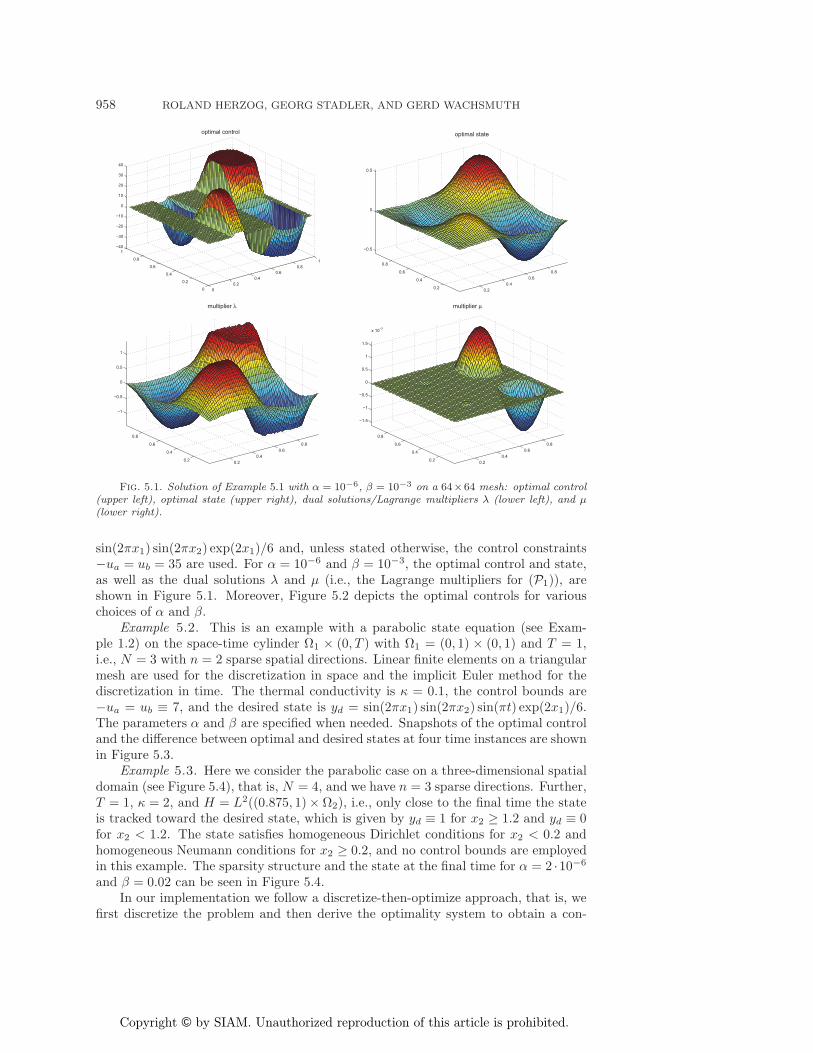
Fig. 5.1. Solution of Example 5.1 with α = 10−6, β = 10−3 on a 64×64 mesh: optimal control(upper left), optimal state (upper right), dual solutions/Lagrange multipliers λ (lower left), and μ(lower right).

sin(2πx1) sin(2πx2) exp(2x1)/6 and, unless stated otherwise, the control constraints−ua = ub = 35 are used. For α = 10−6 and β = 10−3, the optimal control and state,as well as the dual solutions λ and μ (i.e., the Lagrange multipliers for (P1)), areshown in Figure 5.1. Moreover, Figure 5.2 depicts the optimal controls for variouschoices of α and β.

Example 5.2. This is an example with a parabolic state equation (see Exam-ple 1.2) on the space-time cylinder Ω1 × (0, T ) with Ω1 = (0, 1) × (0, 1) and T = 1,i.e., N = 3 with n = 2 sparse spatial directions. Linear finite elements on a triangularmesh are used for the discretization in space and the implicit Euler method for thediscretization in time. The thermal conductivity is κ = 0.1, the control bounds are−ua = ub ≡ 7, and the desired state is yd = sin(2πx1) sin(2πx2) sin(πt) exp(2x1)/6.The parameters α and β are specified when needed. Snapshots of the optimal controland the difference between optimal and desired states at four time instances are shownin Figure 5.3.

Example 5.3. Here we consider the parabolic case on a three-dimensional spatialdomain (see Figure 5.4), that is, N = 4, and we have n = 3 sparse directions. Further,T = 1, κ = 2, and H = L2((0.875, 1)× Ω2), i.e., only close to the final time the stateis tracked toward the desired state, which is given by yd ≡ 1 for x2 ≥ 1.2 and yd ≡ 0for x2 < 1.2. The state satisfies homogeneous Dirichlet conditions for x2 < 0.2 andhomogeneous Neumann conditions for x2 ≥ 0.2, and no control bounds are employedin this example. The sparsity structure and the state at the final time for α = 2 ·10−6

and β = 0.02 can be seen in Figure 5.4.In our implementation we follow a discretize-then-optimize approach, that is, we

first discretize the problem and then derive the optimality system to obtain a con-



00.2

0.40.6

0.81

0

0.2

0.4

0.6

0.8

1−40

−30

−20

−10

0

10

20

30

40

optimal control

00.2

0.40.6

0.81

0

0.2

0.4

0.6

0.8

1−40

−30

−20

−10

0

10

20

30

40

optimal control

00.2

0.40.6

0.81

0

0.2

0.4

0.6

0.8

1−80

−60

−40

−20

0

20

40

60

80

optimal control

00.2

0.40.6

0.81

0

0.2

0.4

0.6

0.8

1−150

−100

−50

0

50

100

150

optimal control

Fig. 5.2. Optimal controls for Example 5.1 for different values of α and β. Upper row: α =10−6, and β = 10−4 (left) and β = 2 · 10−3 (right). The optimal control for β = 10−3 can be seenin Figure 5.1. Lower row: Results without control constraints for β = 10−4, and α = 10−6 (left)and α = 10−8 (right).

Fig. 5.3. Optimal control u (top) and residual yd − y (bottom) for Example 5.2 with α =3 · · · 10−4, β = 5 · 10−3 at times t = 0.25, 0.5, 0.75 (from left to right).

sistent discrete formulation. The linear systems for the elliptic problem are solvedwith a direct solver. The parabolic examples use the iterative generalized minimalresidual method (GMRES) to solve the Newton linearizations. Since these linear



Fig. 5.4. Example 5.3: Sparsity structure of optimal control (left; on gray elements the optimalcontrol is identically zero) and temperature at final time t = 1 (right).

Table 5.1

Results for Example 5.1 for various α and β on 64× 64 mesh with and without control bounds.The fourth and fifth columns show the sparsity of the optimal control (i.e., the percentage of Ωwhere the optimal control vanishes) and the L2-norm of the difference between optimal and desiredstate, respectively. The number of iterations (#iter) needed by the method described in section 4is shown in the sixth column, where the iteration is terminated when the nonlinear residual dropsbelow 10−8. For the unconstrained case we give in brackets the iteration count for the semismoothNewton method from section 3. The last column points to the figure showing the optimal control.

β α ua, ub Sparsity ‖y − yd‖L2(Ω) #iter Plot of u in Fig.

0 1e-6 yes 0% 5.00e-2 112e-3 1e-6 yes 69% 1.42e-1 18 5.2 (upper right)1e-3 5e-5 yes 45% 1.00e-1 71e-3 1e-6 yes 55% 9.46e-2 14 5.1 (upper left)1e-4 1e-6 yes 23% 5.22e-2 11 5.2 (upper left)1e-4 1e-6 no 31% 1.33e-2 7(6) 5.2 (lower left)1e-4 1e-8 no 43% 1.12e-2 16(15) 5.2 (lower right)

systems are similar to optimality systems from linear-quadratic optimal control prob-lems, they can also be solved using advanced iterative algorithms such as multigridmethods [1, 3].

5.2. Qualitative study of solutions. First, we solve Example 5.1 for differentvalues of the parameters α and β to study structural properties of the solutions.Figure 5.1 allows a visual verification of the complementarity conditions for u, λ, andμ. Note, in particular, that the multiplier λ satisfies |λ|x1,2 ≤ 1 for all x1 ∈ Ω1 but doesnot satisfy |λ| ≤ 1 in a pointwise sense. The results for Example 5.1 are summarizedin Table 5.1 and can be seen in Figures 5.1 and 5.2. Also, for the parabolic problems(Examples 5.2 and 5.3) we study the influence of β on the solution. Results are shownin Figure 5.5 (sparsity patterns for Example 5.2 for different values of β) and in Figure5.4. Recall that for time-dependent problems, our notion of sparsity implies that theoptimal control vanishes for all t ∈ [0, T ] on parts of the spatial domain Ω1. From theresults we draw the following conclusions:

• As β increases, the optimal controls become sparser.• As for problems without sparsity constraints, the parameter α controls thesmoothness of the optimal control.

• Even solutions with significant sparsity are able to track the state close tothe desired state. This is particularly true for problems without control con-straints.



Fig. 5.5. Mesh and sparsity structure of optimal controls for Example 5.2 using 1365 spatialdegrees of freedom and 64 time steps for α = 3 · 10−4 and β = 5 · 10−4 (left), β = 5 · 10−3 (middle),β = 2 · 10−2 (right). At dark gray node points, the optimal controls vanish for all time steps.

Table 5.2

Example 5.2 with α = 10−4, β = 10−3, and ρ = 103. Shown are the number of nonlinear itera-tions #iter for different spatial resolution (#nodes denotes the number of spatial degrees of freedomof the triangulation) and numbers of time steps #tsteps. The nonlinear iteration is terminated assoon as the L2-norm of the residual drops below 10−4. With |B| we denote the number of pointswhere the optimal control is zero for every time step and with |Aa| and |Aa| the number of pointswhere the control constraints are active in the space-time domain.

#nodes #tsteps #iter |B| |Aa| |Ab|102 64 7 80 47 61102 256 7 80 184 237367 64 7 273 242 222367 256 7 273 941 862

1365 64 8 992 864 8691365 256 8 994 3368 3403

• The lower right plot in Figure 5.2 suggests that as α → 0, the optimal con-trols become concentrated on the boundary of the active region B in theabsence of pointwise control constraints. A theoretical analysis of this behav-ior, which requires α = 0 and, hence, a different choice of solution spaces (as,for instance, in [8]) might be worthwhile.

5.3. Performance of semismoothNewton methods. Both algorithms basedon semismooth Newton methods prove to be very efficient to solve (P1) for largeranges of the parameters α and β. This can be seen from the number of iterationsto solve Example 5.1 as shown in Table 5.1. Note that the iteration number for thedirectional sparsity approach is not significantly larger than that for the solution ofthe problem with control constraints only (first row in Table 5.1). In the absence ofpointwise control bounds, both algorithms performed equally well (see the last tworows in Table 5.1) and converged for all initializations we tested. We found that themodifications (4.10) of the Newton derivative are important for stable convergence ofthe method presented in section 4.

For the solution of the parabolic problems (Examples 5.2 and 5.3), a reduced spaceapproach is used for the numerical solution of (4.3) (using the modification (4.10)),that is, y, p, and λ, are eliminated from the Newton step and the optimal control u isthe only unknown. To allow for this reduction in Example 5.2, the control constraintsare realized through the quadratic penalization (4.11) with penalization parameterρ = 103. In Table 5.2, we show the number of semismooth Newton iterations required



Table 5.3

Example 5.1 with α = 10−6, β = 10−4 on a 64× 64-mesh, solved with the semismooth Newtonmethod in section 3. Shown is the L2-norm of the nonlinear residual resk in the kth iteration.

k 0 1 2 3 4 5 6resk 3.72e3 2.18e1 8.28e0 3.53e0 1.04e0 6.30e-2 7.93e-13

to solve the problem for different spatial and temporal resolutions. The iteration isterminated as soon as the L2-norm of the nonlinear residual drops below 10−4. Notethat the number of Newton iterations (and thus linear solves) remains approximatelyconstant as the spatial and the temporal resolution increases.

Finally, in Table 5.3 we show the iteration behavior of the nonlinear residualduring the solution of Example 5.1 with α = 10−6 and β = 10−4. Note that the resultshows superlinear convergence of the semismooth Newton method.

6. Conclusion and discussion. In this paper we considered a new class ofnonsmooth control cost (regularization) terms for optimal control problems for PDEs.These terms promote sparsity of the optimal control in preselected directions of theunderlying domain of definition. This behavior is confirmed by numerical examples.Two methods of semismooth Newton type were proposed for the solution of problemsof this new class. In the absence of pointwise control bounds, a complete proof oflocal superlinear convergence was given for the first method. Both methods provedto be very efficient in practice.

Some questions are still open and provide opportunities for further research. Asuitable formulation of the optimality system in the presence of pointwise controlbounds which would allow a rigorous semismooth Newton analysis in function spaceis lacking. Related to this is the question of which reformulations of the optimalityconditions lead to the most efficient and stable algorithm. Moreover, a priori errorestimates, as given, for instance, in [5, 32] for related problem classes involving the“undirected” sparsity term L1(Ω), are not yet available for the problems consideredhere. Finally, the extension to semilinear PDEs and in particular the study of second-order optimality conditions present another challenge.

REFERENCES

[1] S. S. Adavani and G. Biros, Multigrid algorithms for inverse problems with linear parabolicPDE constraints, SIAM J. Sci. Comput., 31 (2008), pp. 369–397.

[2] M. Bergounioux, K. Ito, and K. Kunisch, Primal-dual strategy for constrained optimalcontrol problems, SIAM J. Control Optim., 37 (1999), pp. 1176–1194.

[3] A. Borzı and V. Schulz, Multigrid methods for PDE optimization, SIAM Rev., 51 (2009),p. 361.

[4] E. Candes and Y. Plan, Near-ideal model selection by l1 minimization, Ann. Statist., 37(2009), pp. 2145–2177.

[5] E. Casas, R. Herzog, and G. Wachsmuth, Optimality conditions and error analysis of semi-linear elliptic control problems with L1 cost functional, SIAM J. Optim., to appear.

[6] T. F. Chan and X.-C. Tai, Identification of discontinuous coefficients in elliptic problemsusing total variation regularization, SIAM J. Sci. Comput., 25 (2003), pp. 881–904.

[7] X. Chen, Z. Nashed, and L. Qi, Smoothing methods and semismooth methods for nondiffer-entiable operator equations, SIAM J. Numer. Anal., 38 (2000), pp. 1200–1216.

[8] C. Clason and K. Kunisch, A duality-based approach to elliptic control problems in non-reflexive Banach spaces, ESAIM Control Optim. Calc. Var., 17 (2011), pp. 243–266.

[9] A. Defant and K. Floret, Tensor Norms and Operator Ideals, North-Holland Math. Stud.176, North-Holland, Amsterdam, 1993.

[10] N. Dinculeanu, Vector Measures, Deutscher Verlag der Wissenschaften, Berlin, 1966.



[11] D. Donoho, Compressed sensing, IEEE Trans. Inform. Theory, 52 (2006), pp. 1289–1306.[12] D. Donoho, For most large underdetermined systems of linear equations the minimal �1-norm

solution is also the sparsest solution, Comm. Pure Appl. Math., 59 (2006), pp. 797–829.[13] M. Fornasier, R. Ramlau, and G. Teschke, The application of joint sparsity and total

variation minimization algorithms in a real-life art restoration problem, Adv. Comput.Math., 31 (2009), pp. 301–329.

[14] M. Fornasier and H. Rauhut, Recovery algorithms for vector-valued data with joint sparsityconstraints, SIAM J. Numer. Anal., 46 (2008), pp. 577–613.

[15] E. Haber, L. Horesh, and L. Tenorio, Numerical methods for experimental design of large-scale linear ill-posed inverse problems, Inverse Problems, 24 (2008), p. 055012.

[16] M. Hintermuller, K. Ito, and K. Kunisch, The primal-dual active set strategy as a semis-mooth Newton method, SIAM J. Optim., 13 (2002), pp. 865–888.

[17] M. Hintermuller, S. Volkwein, and F. Diwoky, Fast solution techniques in constrainedoptimal boundary control of the semilinear heat equation, Internat. Ser. Numer. Math.,155 (2007), pp. 119–147.

[18] M. Hladnik and M. Omladic, Spectrum of the product of operators, Proc. Amer. Math. Soc.,102 (1988), pp. 300–302.

[19] S. Hueber, G. Stadler, and B. I. Wohlmuth, A primal-dual active set algorithm for three-dimensional contact problems with Coulomb friction, SIAM J. Sci. Comput., 30 (2008),pp. 572–596.

[20] A. D. Ioffe and V. M. Tichomirov, Theorie der Extremalaufgaben, VEB Deutscher Verlagder Wissenschaften, Berlin, 1979.

[21] K. Ito and K. Kunisch, The primal-dual active set method for nonlinear optimal controlproblems with bilateral constraints, SIAM J. Control Optim., 43 (2004), pp. 357–376.

[22] J. Liu, S. Ji, and J. Ye, SLEP: Sparse Learning with Efficient Projections, Arizona StateUniversity, Tempe, AZ, 2009.

[23] M. Nikolova, Local strong homogeneity of a regularized estimator, SIAM J. Appl. Math., 61(2000), pp. 633–658.

[24] M. Nikolova, Analysis of the recovery of edges in images and signals by minimizing nonconvexregularized least-squares, Multiscale Model. Simul., 4 (2005), pp. 960–991.

[25] Z. Qin, K. Scheinberg, and D. Goldfarb, Efficient Block-Coordinate Descent Algorithmsfor the Group Lasso, Technical report 2806, Optimization Online, 2010.

[26] G. Stadler, Elliptic optimal control problems with L1-control cost and applications for theplacement of control devices, Comput. Optim. Appl., 44 (2009), pp. 159–181.

[27] D. Sun and J. Han, Newton and quasi-Newton methods for a class of nonsmooth equationsand related problems, SIAM J. Optim., 7 (1997), pp. 463–480.

[28] F. Troltzsch, Optimal Control of Partial Differential Equations: Theory, Methods and Ap-plications, Grad. Stud. Math. 112, American Mathematical Society, Providence, RI, 2010.

[29] J. A. Tropp and S. J. Wright, Computational methods for sparse solution of linear inverseproblems, Proc. IEEE, 98 (2010), pp. 948–958.

[30] C. R. Vogel, Computational Methods for Inverse Problems, SIAM, Philadelphia, 2002.[31] G. Vossen and H. Maurer, On L1-minimization in optimal control and applications to

robotics, Optimal Control Appl. Methods, 27 (2006), pp. 301–321.[32] G. Wachsmuth and D. Wachsmuth, Convergence and regularization results for optimal con-

trol problems with sparsity functional, ESAIM Control Optim. Calc. Var., 17 (2011),pp. 858–886.

[33] G. Wachsmuth, Elliptische Optimalsteuerungsprobleme unter Sparsity-Constraints, Diplomathesis, Technische Universitat Chemnitz, 2008; also available online from http://www.tu-chemnitz.de/mathematik/part dgl/publications.php.

[34] S. J. Wright, R. D. Nowak, and M. A. T. Figueiredo, Sparse reconstruction by separableapproximation, IEEE Trans. Signal Process., 57 (2009), pp. 2479–2493.

Date post:	05-Jul-2018
Category:	Documents
Upload:	doantruc
View:	216 times
Download:	0 times

ONTROL OPTIM c - Courant Institute of Mathematical …stadler/papers/HerzogStadlerWach...S u−y d 2...

Documents