DEPARTMENT OF THE INTERIOR U. S. GEOLOGICAL SURVEY RESPONSE SPECTRUM TECHNIQUES FOR PREDICTING WIND-INDUCED VIBRATIONS AND DISCOMFORT IN HIGH-RISE BUILDINGS Part 1- Along-wind direction vibrations E. §afak United States Geological Survey Menlo Park, California, USA E. Uzgider, and A. §anli Istanbul Technical University Istanbul, Turkey Open-File Report 90-19 This report is preliminary and has not been reviewed for conformity with U.S. Geological Survey editorial standards. Any use of trade, product, or firm names is for descriptive purposes only and does not imply endorsement by the U.S. Government. January 1990
Transcript
DEPARTMENT OF THE INTERIOR
U. S. GEOLOGICAL SURVEY
RESPONSE SPECTRUM TECHNIQUES FORPREDICTING WIND-INDUCED VIBRATIONS AND
DISCOMFORT IN HIGH-RISE BUILDINGS
Part 1- Along-wind direction vibrations
E. §afakUnited States Geological Survey
Menlo Park, California, USA
E. Uzgider, and A. §anliIstanbul Technical University
Istanbul, Turkey
Open-File Report 90-19
This report is preliminary and has not been reviewed for conformity with U.S. Geological Survey editorial standards. Any use of trade, product, or firm names is for descriptive purposes only and does not imply endorsement by the U.S. Government.
January 1990
TABLE OF CONTENTS
ABSTRACT ............................... 2
ACKNOWLEDGMENT ......................... 3
1. INTRODUCTION ........................... 4
2. WIND FORCES IN HIGH-RISE BUILDINGS .............. 5
2.1. Models of wind velocity near ground ................. 5
2.2. Wind forces in the along-wind direction ................ 8
3. DYNAMIC RESPONSE OF HIGH-RISE BUILDINGS ........... 9
4. RESPONSE TO WIND LOADS ..................... 11
5. RESPONSE SPECTRA FOR EARTHQUAKE LOADS .......... 15
6. RESPONSE SPECTRA FOR WIND LOADS ............... 17
6.1 A reference building for wind spectra ................. 18
6.2 Modal participation factors for wind spectra .............. 20
6.2.1 Case-1: Pressures are spatially uncorrelated ............ 21
6.2.2 Case-2: Pressures are fully correlated ............... 22
7. MODIFICATION OF EXISTING COMPUTER PROGRAMS ....... 24
8. EXAMPLES FOR WIND RESPONSE SPECTRA ............. 24
9. USE OF WIND TUNNELS FOR WIND RESPONSE SPECTRA ...... 25
10. COMFORT SPECTRA ........................ 26
11. JOINT DESIGN SPECTRA FOR WIND AND EARTHQUAKES ..... 26
12. SUMMARY AND CONCLUSIONS ................... 27
REFERENCES ............................. 28
ABSTRACT
Current methods of building design for dynamic wind loads are based on the equivalent
static load concept, where the dynamic components of wind loads are converted to an
equivalent static load, under which the static deflection is equal to the dynamic deflection.
In the equivalent static load approach, accelerations of the building cannot be incorporated
in the design, because of their dynamic nature. It is well known, however, that in high-
rise buildings wind induced discomfort due to excessive accelerations in the upper stories
can be a problem. Thus, there is a need for a design procedure which can include peak
accelerations as well as peak displacements.
In this report, we present one such method, the response spectrum method, for pre
dicting the wind-induced dynamic response of high-rise buildings. The technique is similar
to that used for earthquake loads, and incorporates not only peak displacements, but also
peak accelerations of the building. In this report, only along-wind direction forces and
vibrations are considered. The across-wind direction response will be considered in the
second part of the research. We develop wind response spectra for a reference building,
defined as a single-degree-of-freedom rectangular rigid block with a rotational base spring
and a damper. We then show that, for a given building, we can calculate peak modal
displacements and accelerations in terms of those of the reference building. We present
wind response spectra for different wind and terrain conditions, and perform a parametric
analysis to investigate the effect of various parameters on these spectra. We show that
existing computer programs that perform spectral analysis for earthquake loads can easily
be modified to perform spectral analysis for wind loads.
We also introduce the concept of comfort spectra. For a given building height, we plot
the acceleration response spectrum and observe the building frequency corresponding to
the critical acceleration for human discomfort. By doing this for a range of building heights,
we can construct an interaction curve showing the building height versus critical frequency.
We call this interaction curve the comfort spectrum, and present several examples. We
conclude by discussing the development of a single design spectrum for earthquake and
wind loads.
11
ACKNOWLEDGMENT
This research has been partially financed by the NATO Collaborative Grants Pro gramme under Grant No 0121/88. The authors wish to acknowledge the support they
received from NATO.
in
1. INTRODUCTION
Wind loading is one of the most important factors to be considered in designing
high-rise buildings. The dynamic component of wind forces have long been recognized
and incorporated in design codes. The current practice of design for wind is based on
the equivalent static load concept, where the dynamic component of the wind load is
converted to an equivalent static load, under which the static deflection of the building
is equal to the dynamic deflection (ANSI, 1982; NBCC, 1985). This load, along with the
static component of wind load, is applied to the building, and a static analysis is performed for design. This approach is known as the gust factor approach (Davenport, 1961). The
design criterion for the gust factor method is to limit the stresses and deflections, the
same as for any other static load, since the method is based on the equivalent static
load concept. It is well known, however, that one of the major problems in high-rise
buildings is the wind-induced discomfort of occupants. Occupant discomfort occurs due
to excessive accelerations, rather than deflections. This observation suggests that the
wind design criterion of high-rise buildings should be based on peak accelerations, as well as peak displacements. Current codes do not have any provisions for wind-induced
peak accelerations. Using existing theory, analytical expressions can be developed for
peak accelerations (e.g., Simiu and Scanlan, 1978; §afak and Foutch, 1987). However, the
expressions are probably too complex to use for practicing design engineers. There is a need
for a simple wind design methodology that will not only incorporate peak displacements and peak accelerations but also will be consistent with the current methods of analysis, so
that design engineers can easily adopt it.
One such method is the response spectrum method. The response spectrum method
has been widely used for earthquake design, and is well known among engineers. It is very
simple, and can incorporate peak accelerations, velocities, and displacements. It was first
suggested by Newmark (1966), and Cevallos-Candau (1980) showed that the earthquake
and wind loads, and corresponding building responses, have a lot of similarities. Therefore, similar methods of analysis, such as the response spectrum technique, can be used for both loads. An important advantage of using the response spectrum technique for both wind and earthquake loads is that when both loads need to be considered for design, the designer
would know beforehand which load will dominate his design, without doing a separate
analysis for each load.
In this report, we present the response spectrum technique for predicting wind-induced
response of high-rise buildings. The technique is similar to that used for earthquake loads,
and incorporates not only peak displacements, but also peak accelerations of the building. Therefore, the method can be used for design for safety (i.e., considers peak displacements),
and also for design for comfort (i.e., considers peak accelerations). We first outline current
1
techniques used for wind and earthquake response analysis of structures. We then show how
the random vibration technique used for wind loads can be put into a response spectrum
form. We present wind response spectra for different wind and terrain conditions, and
perform a parametric analysis to investigate the effect of various parameters on spectra.
We show that existing computer programs that perform spectral analysis for earthquake
loads can easily be modified to also perform spectral analysis for wind loads. We introduce
a comfort spectrum, by which a designer can determine whether the building will be
susceptible to wind-induced discomfort. We conclude by investigating the feasibility of
developing a single design spectum for wind and earthquake forces.
2. WIND FORCES ON HIGH-RISE BUILDINGS
Wind-induced vibrations in high-rise buildings are due to individual or combined
effects of the following dynamic force mechanisms: along-wind forces due to turbulence, across-wind forces due to vortex shedding, wake buffeting, and galloping. Along-wind
forces are in the direction of main wind flow. They include static and dynamic components,
generated by the steady and fluctuating components of the wind, respectively, and are the most dominant force mechanism in a typical building. In general, along wind forces are
in the form of pressures on the frontal (i.e., windward) face, and suctions on the back (i.e., leeward) face of the building. Across-wind forces are generated by vortecies that
develop at the sides of the building moving clockwise and counterclockwise, and shed in
an alternating fashion in the direction perpendicular to the mean wind flow. Across-wind forces can be critical for slender structures, such as buildings with very large height to width
ratios, smokestacks, and transmission towers. Wake buffeting occurs if one structure is
located in the wake of another structure, and can cause large oscillations in the downstream
structure if the two structures are similar in shape and size, and less than ten-diameter
apart. Galloping is an oscillation induced by forces generated by the motion itself. It
corresponds to an unstable motion with negative damping, and can be seen in structures
like transmission lines, or long slender towers with sharp edged crossections. More detail
on wind force mechanisms can be found in Simiu and Scanlan (1978) and §afak and Foutch (1980). In this study, we will deal only with along-wind forces in the direction of main
wind flow. Forces in the across-wind direction will be considered in the second phase of
the study.
2.1. Models of wind velocity near ground:
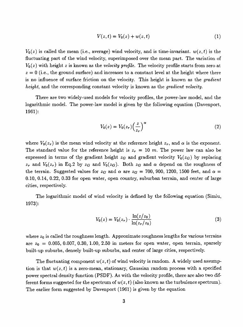
Wind velocity generates all the force mechanisms acting on the structure. Near the ground, the wind velocity V(z, t) at height z can be expressed as the sum of two compo
nents, as shown in Fig. 1, such that
) (1)
VQ(Z) is called the mean (i.e., average) wind velocity, and is time-invariant. w(z,t) is the fluctuating part of the wind velocity, superimposed over the mean part. The variation of
VQ(Z) with height z is known as the velocity profile. The velocity profile starts from zero at z = 0 (i.e., the ground surface) and increases to a constant level at the height where there
is no influence of surface friction on the velocity. This height is known as the gradient
height, and the corresponding constant velocity is known as the gradient velocity.
There are two widely-used models for velocity profiles, the power-law model, and the
logarithmic model. The power-law model is given by the following equation (Davenport,
1961):
(2)
where Vo(zr ) is the mean wind velocity at the reference height zr , and a is the exponent.
The standard value for the reference height is zr = 10 m. The power law can also be
expressed in terms of the gradient height ZG and gradient velocity VQ(ZG} by replacing
zr and VQ(ZT ) in Eq.2 by ZG and VQ(ZG)> Both ZG and a depend on the roughness of
the terrain. Suggested values for ZG and a are ZG = 700, 900, 1200, 1500 feet, and a = 0.10, 0.14, 0.22, 0.33 for open water, open country, suburban terrain, and center of large
cities, respectively.
The logarithmic model of wind velocity is defined by the following equation (Simiu,
1973):
where ZQ is called the roughness length. Approximate roughness lengths for various terrains
are ZQ = 0.005, 0.007, 0.30, 1.00, 2.50 in meters for open water, open terrain, sparsely
built-up suburbs, densely built-up suburbs, and center of large cities, respectively.
The fluctuating component w(z, t) of wind velocity is random. A widely used assump
tion is that w(z,t) is a zero-mean, stationary, Gaussian random process with a specified
power spectral density function (PSDF). As with the velocity profile, there are also two dif ferent forms suggested for the spectrum of w(z, t) (also known as the turbulence spectrum).
The earlier form suggested by Davenport (1961) is given by the equation
1200/
where Vb(10) is the mean wind velocity in meters per second at the reference height of 10
meters, / is the frequency in cycles per second (Hz), and K is the surface drag coefficient.
The value of K varies from 0.005 for open country to 0.05 for city centers. The shape of
Davenport's spectrum is independent of the height, and has a peak at a wave length of 600
meters (i.e., Vb(10)// = 600). This spectrum is currently used in building codes in many
countries.
A later model for the turbulence spectrum is suggested by Simiu (1974), and can
incorporate the variation of the spectrum with height. Simiu's spectrum is given by the
following equation:
"« 2007V fz (5)
where w* is known as the friction velocity, calculated in terms of the reference velocity and
the roughness length by the following equation
*
Since N in Eq.5 is a function of 2, Sw(z,f) is height dependent. A more precise, but
analytically more complicated, form of this spectrum is given in Simiu (1974).
The level of turbulence in a wind flow is described by its turbulence intensity. The
turbulence intensity I(z) is calculated as the ratio of the RMS (root-mean-square) value
of the fluctuating component of wind velocity to the mean component. That is
where crw (z) is the RMS value of w(z,t). From random process theory,
oo
<£(*) = / Sw(z, f)df (8)/=0
For Davenport's spectrum (Eq.4), aw is constant, since the spectrum is independent of 2,
and equal to 6XV02 (10). For tall buildings, the turbulence intensity may vary from 0.05
to 0.30 depending on the building height and the roughness of the terrain.
2.2. Wind forces in the along-wind direction:
Forces in the along-wind direction are generated by the velocity of the wind flow.
Neglecting the relatively small added mass term, the pressure P(z,t) acting at a point of
height z of a fixed body in a turbulent flow can be written as
P(z,t) = \pCp(z)V\z,t) (9)
where V(z, i) is the wind velocity, Cp (z) is called the pressure coefficient, and p is the mass
density of the air. By separating the wind velocity V(z,t) into its mean and fluctuating
components, as in Eq.l, and also neglecting the w'2 (z^i] terms, Eq.9 can be approximated
as
P(z, t) « \pCr(z}V*(z) + PCp(z)V0 (z)w(z, t) (10)
The omision of the i/; 2 (^,t) term is justified since the turbulence intensity is generally
much less than one. The first term on the right hand side of Eq. 10 is independent of
t, therefore it represents the static wind pressure. The second term is the dynamic wind
pressure. Denoting static and dynamic wind pressures by PQ(Z) and p(z,t), respectively,
we can write
P(z,t) = P0 (z)+p(z,t) (11)
where
z)V?(z) and p(*,t) = pCp(z)V0 (z)w(z,t) (12)
Since PQ(Z) is a static load, the response of the structure resulting from this load can be
calculated by using static methods of analysis.
The calculation of the response due to the dynamic pressure p(z,t) requires the ap
plication of random vibration techniques because of the random w(z,t). Since p(z,t) is a
linear function of w(z, t), we conclude that p(z, t) is also a zero-mean, stationary, Gaussian
random variable. Its standard deviation, <fp (z}, and PSDF, 6^(2, /), can be calculated in
terms of those of w(z,t):
op (z) = pCp(z)V0 (z)<rw (z) (13)
and
S,(z,f) = [pCr(z)V0 (z)] 2 Sw(z,f) (14)
5p (^,/) is sufficient to describe fully the stochastic characteristics of p(z,t\
3. DYNAMIC RESPONSE OF HIGH-RISE BUILDINGS
Vibration tests indicate that the behavior of high-rise buildings under dynamic loads
is somewhere between that of a shear beam and a flexural beam. The closed form vibration
equations, assuming a shear beam or a flexural beam model, can be derived in the con
tinuous domain (see, for example §afak and Foutch, 1980). Vibration equations can also
be expressed in a discrete domain by using discrete modeling techniques, such as matrix
methods and finite element methods. We will prefer the discrete approach, so that we can
make use of commercially available computer programs.
We will assume that the motion of the building can be modeled in terms of horizontal
displacements at each story level. The rotations will be neglected, since their contribution
to the response is generally very small (Hurty and Rubinstein, 1964). We will also assume
that the building is symmetric, and moves only in the along-wind direction (we will consider
the motion in the across-wind direction in the second phase of the study). With these
assumptions, the building becomes an n-DOF (n-degrees-of-freedom) dynamic system, n
representing the number of stories. The equations of motion, assuming linear behavior,
can be written as
WWW + lC}{y(t)} + lK}{y(t)} = (F(t)} (15)
In Eq.15, [M], [C], and [K] are n x n mass, damping, and stiffness matrices, respectively,
and {y(t)} and {F(t)} are n-dimensional displacement and force vectors. The dots over y
denote derivatives with respect to time t. The solution of Eq.15 can be accomplished by
using modal analysis techniques. First, assuming that [C] = 0 and {F(t)} = 0 in Eq.15,
we solve the following n-dimensional eigenvalue equation:
[M]{y(t)} + (K}{y(t)} = 0 (16)
Eigenvalues and eigenvectors obtained from the solution of this equation correspond, re
spectively, to n natural frequencies and mode shapes of the building. Using calculated
mode shapes, the displacement vector {y(t)} can be expressed as
(17)
where [$] is a n x n matrix composed of mode shapes (i.e., each column of [$] represents
a mode shape), and {<?(£)} is the n-dimensional generalized coordinate vector representing
the modal amplitudes. In explicit form, the i-th component yi(t) of {y(t}} can be written
where $^ represents the element at the z'-th row and k-th column of matrix [$]. An
important property of vibration mode shapes of an n-DOF system is orhogonality:
= 0 and {3> k }[K]{$ l }=Q for k^l (19)
where {$*} and {$/} are vectors denoting the fc'th and Vth mode shapes, and the super
script T denotes the transpose. If it is assumed that the damping matrix C is a linear
combination of mass and stiffness matrices (i.e., C = cm M -\- c^A"), the orthogonality
property also applies to the damping matrix, that is
{*k}T[C]{$i} = Q for k?l (20)
The orthogonality property can be used to reduce the n-dimensional matrix equation in
Eq.15 to a set of n independent modal equations. Using Eq.17 in Eq.15, and then multi
plying both sides by the transpose of any (e.g., k-th) mode shape vector, and also using
the orthogonality properties (Eqs.19 and 20), we can write for the k-th modal equation of
the motion
(21)
For simplicity, introduce the following notation:
(22)
CJ = {^nCK**} (23)
(24)
(25)
M^, C^, K%, and F£(t} are called the fc-th generalized mass, damping, stiffness, and force,
respectively. To simplify it further, we will write
2 *C*k = 2£o*(27r/o*)M; and tffc* = (27r/ofc )M,* (26)
where fofc is the damping ratio, and /o* is the cyclic frequency for the fc-th mode. With
these, we can write for the fc-th modal equation of the motion as
where Aj denotes the tributary wind exposure area for the j-th story, and x denotes the
horizontal coordinate axis perpendicular to the main wind flow. It is assumed that VQ(Z)
does not change in the horizontal direction. The tributary area Aj can be calculated as
(31)£,
Bj and hj are the width and the story height (with respect to the story below), respectively,
at the j 'th story.
{Pw(t)} can be separated into static and dynamic components, {Po w } and {pw (t)},
such that
{Pw (t)} = {P0w } + [pw (t)} (32)
The j'th components of {Po«;} and {pw (t)} can be written, from Eq.30, as
zj+hi + l /2
P0wj = ^pBj j Cp (z}V2 (z}dz (33)
Zj-hj/2
pwj (t) = P I I Cp(z)V0 (z)w(x, z,t)dxdz (34)
All the other components can be calculated similarly.
Since {PQ W } is a static load, the resulting static response, {t/o}, can easily be calculated
as
POWJ (35)
For the dynamic response, we will first calculate the generalized force vector {F*(t)}. For
the j'th component of {F*(t)}, we can write from Eq.25 that
n
= XI *jkP*,k(t) (36)k=l
where the vector {$j} denotes the j'th mode shape. In Eq.36, the generalized force is given
in a discrete form as the sum of modal amplitudes multiplied by the corresponding dynamic
story forces (i.e., dynamic pressures times the tributary story area). The same equation can
also be written in a continuous form by using integrals instead of sums. We will prefer the
continuous form, since the available information on the stochastic description of dynamic wind loads is all given in the continuous domain. When the mode shapes are available
only in discrete form, we can approximate the continuous mode shapes by connecting the
discrete amplitudes by straight lines. Using Eq.34, we can write for the j'th generalized
modal wind force in the continuous form as
j(z) pCp (z)V0 (z)w(x, z, t) dxdz (37) *i
where $j(z) denotes the continuous j'th mode shape.
Since w(x, z t t) is random, the generalized modal force Fj(t) is also random. Therefore, the calculation of the response requires applications of random vibration techniques. One
popular method for stationary excitations is the spectral analysis technique, where the
response is calculated in terms of PSDF's. For a multi-degree-of-freedom system (e.g.,
Eq.15) with random excitation, the relationship between input and output PSDF's can be written as (Lin, 1976)
Sy (zi,z<2~f] is the cross "PSDF of the responses at points z\ and z<i, and [Sp*(f)] is the
PSDF matrix of the generalized force. {$(21)} and {$(^2 )} denote vectors composed of
modal coordinates at height z\ and 22, respectively.
[H(f)] is the complex frequency response matrix of the structure, calculated by the
equation
(39)
where i= \/--T. [H(f)] denotes the complex conjugate of [H(f)}.
The j,fc component of the PSDF matrix [Sp*(f)} of the generalized force can be
written in the continuous domain from Eq.37 as
= [ fJ J Aj JAk
x 2 dz2 (40)
$ti;(£i , z\ , £2 , 22> /) is tne cross-PSDF of the fluctuating wind velocitiy w(x, z, t), and can
where Sw(z,f) is the PSDF at z, and Coh(xi,z\,x2 , z2 ,f] is the coherence function of
the fluctuating wind velocities at points (#1,2/1) and (x 2 ,y2 ). It is assumed that Sw(z,f)
does not change horizontally (i.e., it is not a function of x). The equation suggested for
Coh(xi,zi,x2 ,z2 ,f) is (Vickery, 1971)
1/21(42)
Cz and Cz are called the exponential decay coefficients. Their suggested values are Cx = 16
and Cz = 10. Experiments show that these values can change significantly, depending on
the terrain, height, and the wind speed, and therefore represent a source of uncertainity
(Simiu and Scanlan, 1978).
By using expressions derived in Eqs. 39-42, the response PSDF, Sy (zi,z2 ,f), is calcu
lated from Eq.38. The integral of Sy(z\,z2 ,f) over the frequency / gives the covariance
matrix, ai (z\, z2 }, of the response. That is
oo
= f (43)
For z\ = z2 = z, &y(z) is the mean square response at z. At a given height 2, the peak
response is calculated as
Oy(*) (44)
where y$(z) is the static response due to static wind load, and gy (z) is known as the
peak (or gust) factor. The peak factor can approximately be calculated by the following
equation (Davenport, 1964):
(45)
v(z) is the average number of peaks in the response y(z) per unit time, and T is the
duration in seconds considered for the excitation and response in peak calculations. A
commonly used value for T is 3600 seconds, corresponding to a one-hour wind storm. v(z)
can be calculated in terms of the PSDF by the equation
11
ffSy(z,f)df"2 W = fs (46)
/ S,(z, f) df0
This approximation is based on the assumption that the response is a narrow band sta
tionary random process with independently arriving peaks.
The accelerations can be calculated by taking the second derivatives of displacements.
The PSDF Sa (zi, ^2? /) of accelerations can be written in terms of the PSDF of displace
ments as
Sa (zi,Z2 J) = (2*f)*Sy ( Zl ,Z2 J) (47)
The covariance function of the accelerations is
00
= f (48)
The peak acceleration at height z is calculated in the same way as the peak displacements
(Eq.44):
maxa(z,£) = ga cra (z) (49)
Note that the mean (i.e., static) acceleration is zero. ga is calculated similar to gy by
replacing ay and Sy in Eqs.44-46 by aa and 5a .
5. RESPONSE SPECTRA FOR EARTHQUAKE LOADS
The response spectrum for earthquakes is a curve that shows the variation of the peak
displacement of a SDOF ( single- degree-of- freedom) oscillator with its natural frequency for
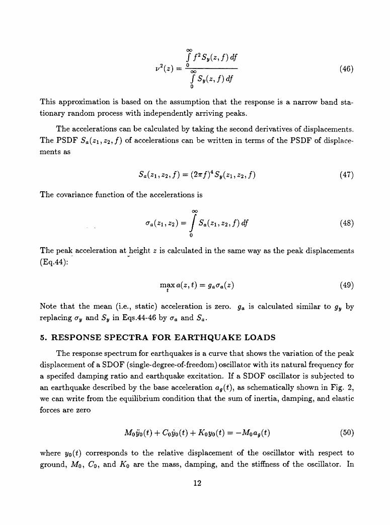
a specifed damping ratio and earthquake excitation. If a SDOF oscillator is subjected to
an earthquake described by the base acceleration ag (t), as schematically shown in Fig. 2, we can write from the equilibrium condition that the sum of inertia, damping, and elastic
forces are zero
M0 y0 (0 + C0yo(0 + K0 y0 (t) = -M0 ag (t) (50)
where yo(t) corresponds to the relative displacement of the oscillator with respect to
ground, MO, Co, and KQ are the mass, damping, and the stiffness of the oscillator. In
12
terms of the natural frequency and damping, we can write the same equation (see Eq.26) as
Equation 50 shows that the effect of earthquake base motion in a SDOF oscillator is
equivalent to applying a ficticious force on the oscillator, defined by the equation
F0 (0 = -M0 ag (t) (52)
Using Duhamel's integral, as in Eq.28, we can write for the displacement (relative to the
base) yo(t) of a SDOF oscillator to earthquake base acceleration ag (t)
t
yo(<) = -^~ j ag (r) h0 (t - r) dr (53)
r=0
where ho(t T) is given by Eq.29. We define the response spectrum -D(/o) for frequency /o as
£>(/<>)= max y0 (0 (54)
The plot of D(fo) with respect to /o gives the response spectral curve. Since the response
yo(0 is dependent on the damping in addition to the excitation, different damping ratios,
£o, and excitations, ag (t), would give different spectral curves.
For multi-story buildings, again considering the relative displacement of the building
with respect to the ground, we can express the load vector as the product of the mass matrix and acceleration vector whose elements are all equal to ground acceleration. That
is,
{F(t)} = -lM]{I}ag (t) (55)
where {/} denotes an n-dimensional unit vector. The generalized force vector given by
Eq.25 then becomes
where A* = -MI (56)
\k is called the participation factor for the fc-th mode, which represents the portion of total load associated with that mode. Using Eq.56 in Eq.28, we can write for the Ar-th
modal response qk(t) of a building subjected to ground acceleration ag (t)
13
(57)r=0
By comparing Eq.57 with Eq.53, we note that the right hand side of Eq.57 is equivalent
to the response of a SDOF oscillator except the constant term \k/M£. Therefore the peak
fc'th modal response is equal to that of a SDOF oscillator corresponding to mode k (i.e.,
the amplitude of the response spectrum for damping £ofc at frequency /ojt) multiplied by
A fc /M£. That is
/\ JL At
maxqk (t) = - maxy0 (<) = -^ D(fok ) (58)
For each mode, peak modal responses can be calculated similarly by using the response
spectrum. Although the response at any given time can be written in terms modal re
sponses (Eq.17), the same is not true for the peak response, because the peak modal
responses do not necessarily occur at the same time. In other words, the peak response is
not equal to, but less than, the sum of peak modal responses. Various methods have been
used to approximate peak response in terms of peak modal responses, such as the absolute
sum, the -square root of the sum of the squares, or the quadratic combination.
6. RESPONSE SPECTRA FOR WIND LOADS
Development of response spectra for wind loads can be accomplished following a sim
ilar approach to that for earthquake loads. Wind response spectra should be defined for a
given site, since the velocity and turbulence structure of the wind is strongly site depen
dent. Earthquake loads are inertia loads. Therefore the spectral response involves only the
damping and the natural frequency of a structure and not any other structural parameter.
Wind loads, however, are strongly dependent on the outside geometry of the structure. It
is the size and the shape of the wind exposure area that determine the total wind load
on the building. Therefore, wind response is dependent not only on the natural frequency
and damping, but also on the outside geometry of the structure. Since we are dealing with
buildings with rectangular cross-sections and normally incident wind, and also considering
only along-wind vibrations at this phase of the study, we can define the outside geometry
with the height and frontal width of the building. Further simplification can be achieved
for very tall buildings by neglecting the variation of wind pressures in the horizontal di
rection and using pressure coefficients averaged over the frontal width. For such buildings,
the outside geometry is represented only by the height of the building. In the formulation
that follows we will consider both the height and the width of the building. We will define
14
wind response spectra for a given site, and given structural damping, height, and height-
to-width ratio. The dependence of wind response spectra on height and height-to-width
ratio is the major difference when compared to earthquake response spectra.
6.1. A reference building for wind spectra;
In order to develop wind response spectra, we will consider a reference building as
schematically shown in Fig. 3. The reference building can be visualized as a rigid block
of specified width, height, and mass, connected to the base by a rotational spring-dashpot
system. Therefore, the reference system is a SDOF system, and its single mode shape is a
straight line. We will develop wind response spectra for the reference system for different
damping ratios, wind velocities, heights, and height-to-width ratios. We will assume unit
mass per unit height, and a location in the middle of a city.
Using the coordinate system shown in Fig. 3, we can write for the response of the
reference system as
where $r (z) denotes the single mode shape of the system. Since the building has only one
degree of freedom, a rigid body rotation with respect to the base, we can write for the
mode shape
*r« = jj (60)
The equation for qr (t), similar to Eq.28, is
qr\l) i ^sOr\^""yOrJ9r\" ) i (.^^jOr) 9rv*J = %~f~~~ v /lvl r
where £or and /o r are the damping ratio and natural frequency, and F* and M* are the
generalized load and mass of the reference building, respectively. For unit mass per unit
height, we can calculate the generalized mass of the reference system as
H H
M; = /*fc) -1 dz = I(±-} 2 dz = %. (62)
Using Eqs.38-41, we can write for the PSDF, Syr (zi,Z2-> f}, of the displacement response
of the reference system
15
2) /) (63)
The PSDF for the accelerations is
Sar (zl ,z2 ,f) = (2,fYSyr (z,,z2 ,f) (64)
The RMS displacement cryr (H), and the RMS acceleration crar (H) at the top of the building are
00 00
= Jsyr (HJ)df and aar (H) = J Sar (HJ)df (65) yr
0
For the peak displacement, maxyr (H, £), and the peak acceleration max ar (#,£), at theI I
top, we can write (see, Eqs.44-49)
max yr (H, t) = y0r (H) + gyr (H)ayr (H) (66)
max ar (H, t) = gar (H)crar (H) (67)Z
where yo r (H) is the static displacement due to static wind load, and gyr (H) and gar(H) are the displacement and acceleration peak factors, respectively, at the top of the referencesystem.
For the displacement response spectra, we will only consider the dynamic displace ment, since the static displacement can easily be calculated using static analysis. It should be noted here that, if desired, the static displacement can also be included in the response spectrum by expanding it into static modal components. We will define the displacement response spectra as the plot of the peak dynamic displacement response at the top of the reference building against the natural frequency for a range of frequencies. Therefore, for the natural frequency /QJ the displacement spectra, D(/oj), is
. = gtr (H)ff,T (H) (68)dynamic
Similarly for the acceleration spectra, we can write
16
= gar(H)aar (H) (69)
6.2. Modal participation factors for wind spectra:
In order to calculate the wind response of a given building by using the response
spectra of the reference building, we first have to determine the modal participation factors.
The modal participation factor will be defined as the ratio of the peak modal response of
a given system to that of the reference system that has the same modal frequency and
damping.
The PSDF, Syj(f), of the j-th modal displacement of a given building is (from Eq.38)
(70)
where Hj(f), the frequency response function for the j-th mode, can be written from Eq.39
Bj(f) = f - T (71) MJ [-(2ir/)» + i(
SF? (f) can be calculated from Eq.40 by putting j = k. Similarly, the PSDF of the reference
system, 5rj(/), corresponding to j-th mode (i.e., the reference system with frequency /QJ,
damping £o>, and same outside dimensions) is
STi (z,f) = *(*)|JM/)|Si7//) (72)
The frequency response function of the reference system, Hrj , is the same as that of the
actual system for the j'th mode, Hj(f), except the scaling factor (i.e., the mass term).
The relationship can be written as
M*(73)
Since the loading on the reference and actual systems are the same, and their frequency
response functions are equal to within a scaling factor, we conclude that the spectral con
tents of the modal response and the response of the corresponding reference system are the
same. Therefore the peak factors for each response can be assumed equal. Consequently,
the ratio of the peak modal response to the peak response of the corresponding reference
system is equal to the ratio of their RMS responses. If we denote this ratio by kj(z) for
the responses at height z, we can write
17
a'iw ISrj(z,f)df0
Because of the four-fold integration involved in the calculations of SF* (/) and SF*.
(see Eq.40), a straightforward evaluation of kj(z) is very complicated, and would not
have much practical use. To simplify the calculations, we will consider two extreme cases
regarding the spatial correlation of the pressures. Case 1 will refer to the situation where
the pressures are spatially uncorrelated, whereas Case 2 will refer to the situation where
the pressures are fully correlated. In addition, we will assume that the PSDF of the velocity fluctuations is independent of the height as suggested by Davenport (1961). The simplifed
expressions for kj(z) can then be developed as follows:
6.2.1. Case 1: Pressures are spatially uncorrelated
If the pressures are uncorrelated we can assume that
For Case 1, from Eq.74 and also using Eq.73, the ratio of the top-story RMS responses
becomes
li( ' ~Mr*
(80)
6.2.2. Case 2: Pressures are fully correlated
If the pressures are fully correlated, the coherence function is unity, that is
Coh(xi,zi,x2 ,z2 ,f) - I
The PSDF of the generalized force (Eq.40) then becomes
(81)
(82)
Using the same approximation as in Case 1 for Cp(z), we can write for the PSDF of the
j-th modal response at the top
H
(83)
and similarly for the reference system
Srj (HJ) = r (H)(PCDB^\Hrj
The ratio of the RMS responses, k%j, becomes
H
(84)
* Sr 0*H
> /0
19
As stated earlier, since the peak factors for the modal response and the corresponding
reference system response are equal, these ratios are also valid for the peak responses.
Therefore, the peak value of the j-th modal response at the top, maxyj(#, £), can be
calculated in terms of the response ratio and the peak response of the reference system as
m&xyj(H,t) = kj(H)m&xyr(H,t) (86)T t
Since we defined maxyr (#, t) as the spectral response (Eq. 68), we can calculate the peak
modal response as
) = kj (H)D(foj ) (87)
The total peak response can be approximated by combining peak modal responses. If
SRSS (square-root-of-sum-of-squares) method is used for the combination, the total peak
response becomes
1/2(88)
The "equations for accelerations are similar. Since the relationship between acceler
ations and displacements is a function of frequency only (see Eq.47), the ratios kij and
&2j calculated for displacements are also valid for the accelerations. Therefore, we can
calculate the peak top-story acceleration for the j-th mode, maxaj(#, t] in terms of the
spectral acceleration of the reference system as
max a.j(H, t) = kj (H)A(foj ) (89)
The total peak acceleration is obtained by combining the peak modal accelerations as in
Eq.88.
For a given building, the value of kj(z) is somewhere between kij(z) and k2j(z). We
have no way of knowing the exact values without explicitly incorporating the correlation
structure of the wind. Therefore, an approximation needs to be made regarding which value
to use for kj(z). For the first mode, the two values would be very close since the first mode
shape in most buildings is almost a straight line, the same as that of the reference building.
For higher modes, the ratio kij(z) would always be larger than the ratio k2j(z), because
the value of the integral / $*(z)V£(z)dz is always larger than that of f$j(z)Vo(z)dz (the
negative portions of mode shapes become positive in the first integral due to the square),
whereas the values for the integrals f $*(Z)VQ(z)dz and f $r(z)Vo(z)dz are always close.
20
Therefore, for higher modes kij(z) can be considered as the upper bound, while &2j(<z) is
the lower bound. We suggest that an average value calculated as
*, = ^±^ (90)
is an appropriate one.
7. MODIFICATION OF EXISTING COMPUTER PROGRAMS
There is a large number of commercially available computer programs that can perform
free vibration analysis. These programs can easily be extended to perform dynamic wind
analysis by using the spectral analysis method presented above. In order to do this, we
first have to generate a set of response spectra that includes spectral curves for different
meteorological (e.g., mean wind velocities, turbulence levels, etc.), and structural (e.g.,
damping, width, height) conditions, as will be shown in the next section.
To estimate the dynamic wind response of a given building, we determine the natural
frequencies, mode shapes, and generalized masses of the building by performing free vibra
tion analysis. We then add a subroutine to the program to compute the ratios k\j(z] and
k2j(z) and the average ratio kj(z) from Eqs.80, 85, and 90 for the velocity model selected.
Note that only the shapernot the exact amplitudes, of the velocity profile is required in the
calculations. The mode shape and the generalized mass for the reference system are given
by Eqs.60 and 62. For each modal frequency and damping we take the spectral amplitude
from the corresponding response spectra, and multiply it by the modal participation factor
to obtain peak modal responses. We then combine the peak modal responses according to
Eq.88 to obtain the total peak response.
8. EXAMPLES FOR WIND RESPONSE SPECTRA
In this section we develop a set of displacement and acceleration response spectra
for a location assumed to be the center of a city. We consider three wind velocities,
three building heights, three height-to-width ratios, and two damping ratios, resulting in
3x3x3x2 = 54 spectral curves for the displacements and accelerations. The frequency
range used in the spectra is 0.1 Hz to 2.0 Hz with 0.1 Hz increments (20 values).
For the wind velocity structure, we assume the velocity profile and the PSDF suggested
by Simiu (1973, 1974). The three mean wind velocities considered, at the reference height
zr = 10 m., are Vo(10) = 50, 80, and 100 km/h. The roughness length, z0 (Eq.3) was
chosen 0.5 m., a value representative of a city center. The friction velocity u* for each
Vo(10) was calculated from Eq.6. The velocity spectrum used corresponds to a turbulence
level, such that <7^ = 6uJ. The pressure coefficient taken as Cp (z) = 1.3, which is assumed
21
to be the sum of the pressure coefficient on the front face (taken as 0.8), and the suction
coefficient on the back face (taken as 0.5). It is assumed that this value represents the
averaged value over the building (i.e., CD = Cp (z) = 1.3 in Eq.77). The exponential decay
coefficients of the coherence function (Eq.42) were chosen as Cx = 16 and Cz = 10. The
mass density of the air is p = 1.25 kg/m3 .
As for the structural parameters, we consider three heights, H = 100, 200, 300 m.,
and for each height, three height-to-width ratios, H/B = 2, 4, 6. The damping ratios
used are 0.02 and 0.05. We also assumed unit mass per unit height. Since only alongwind
direction forces and displacement are considered, the third dimension of the building (i.e.,
the depth) is not needed in the calculations.
For every combination of wind and structural parameters given above, the peak dis
placement and acceleration at the top of the building were calculated for frequencies from
0.1 to 2.0 Hz with 0.1 Hz intervals. The resulting spectral curves are plotted in Figs.
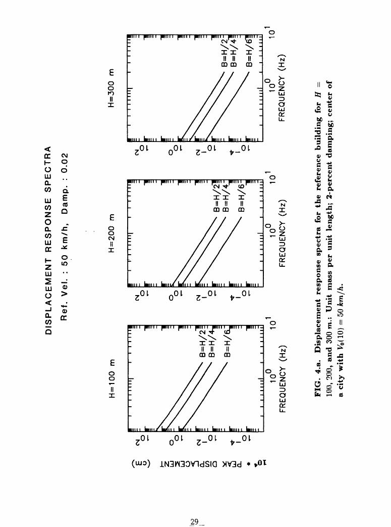
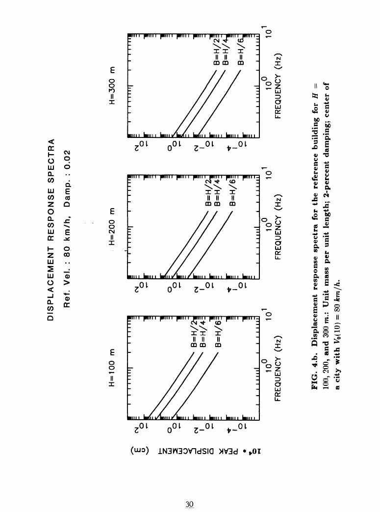
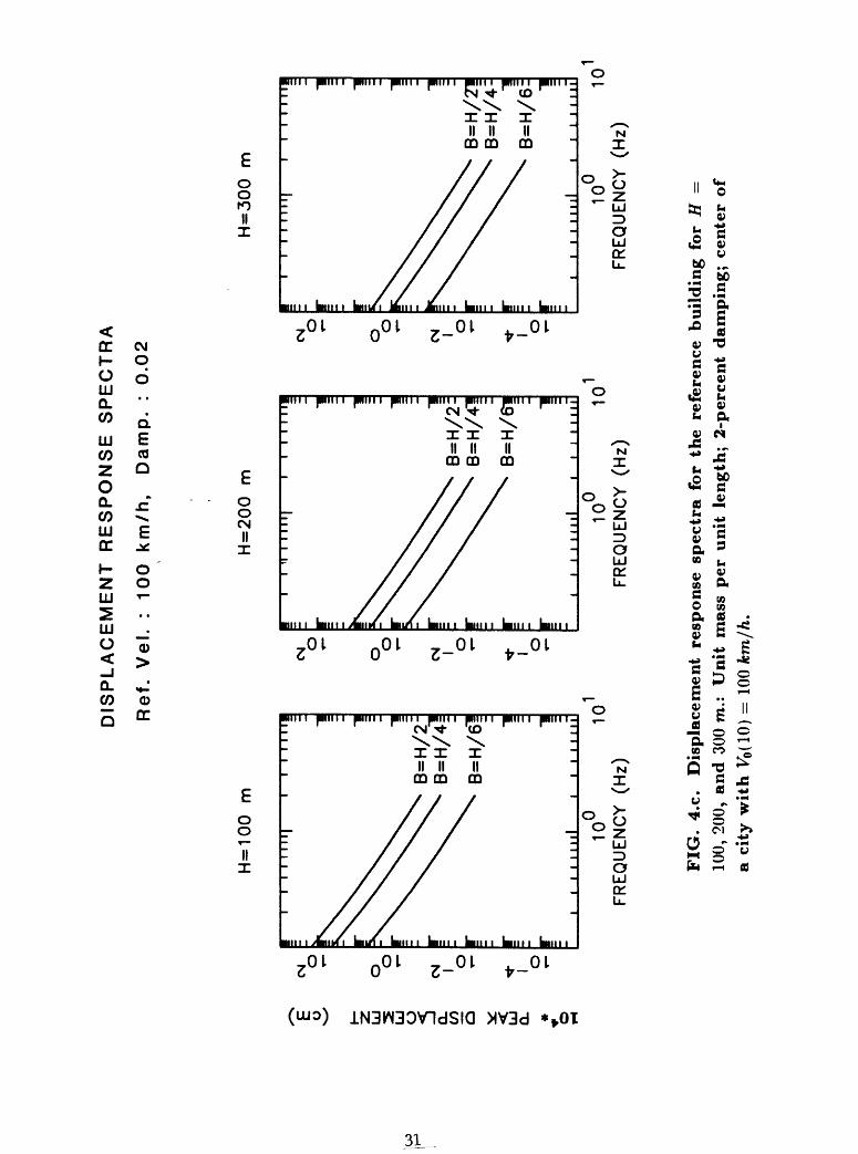
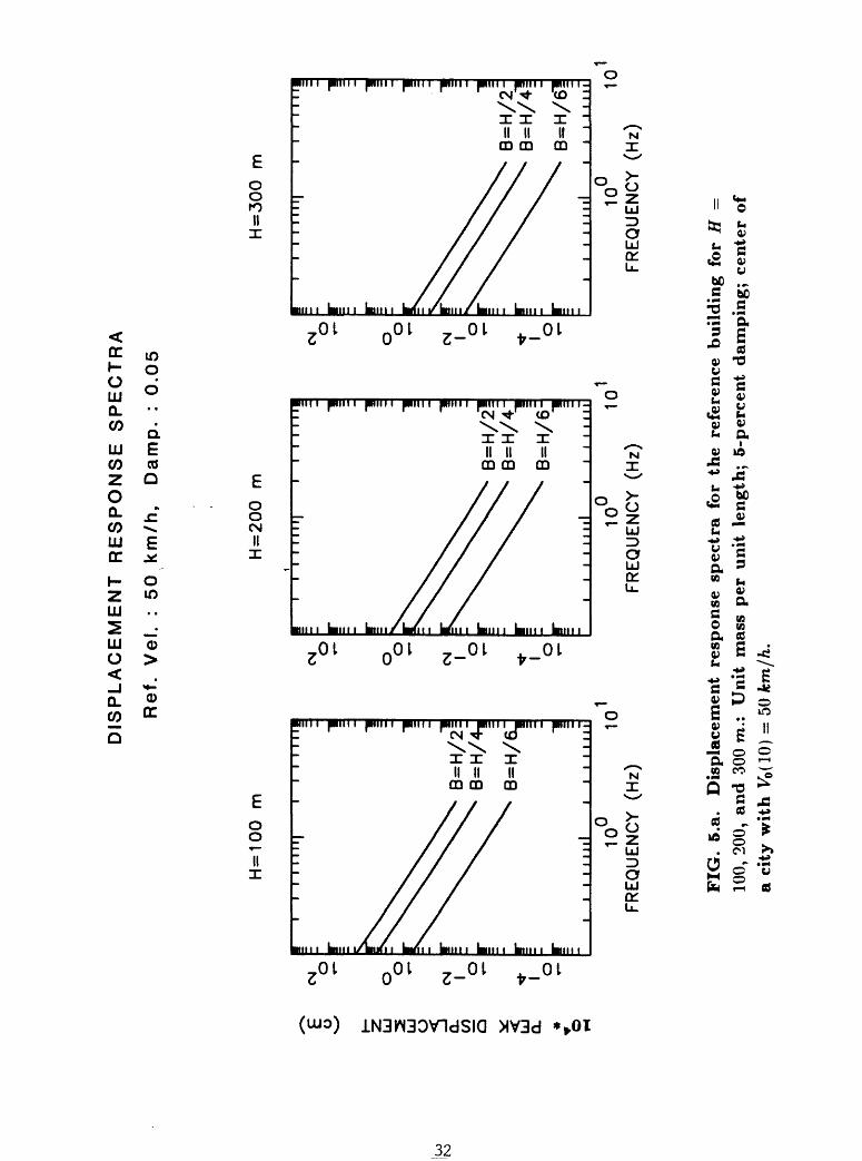
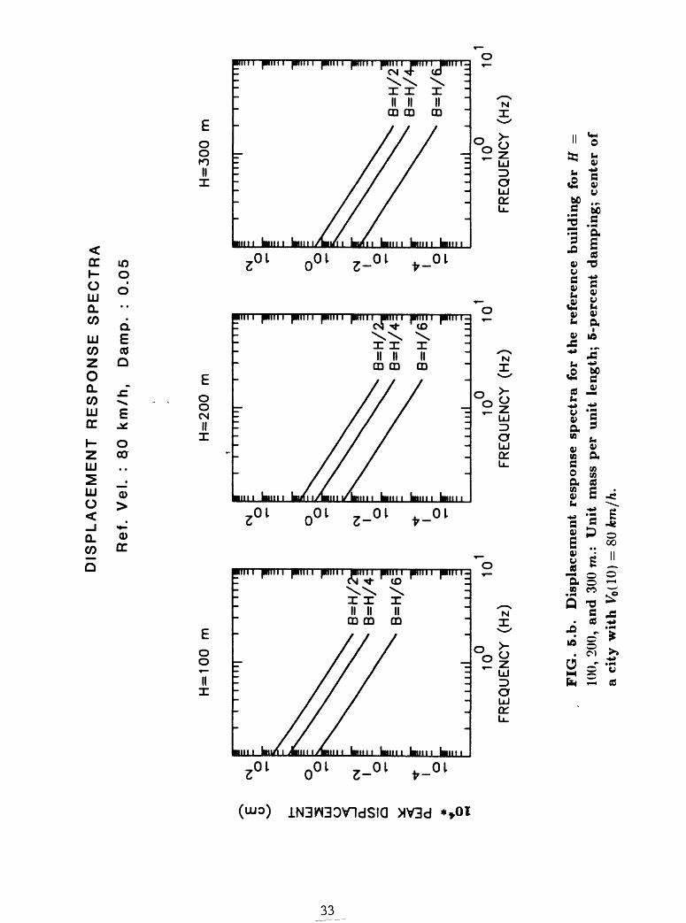
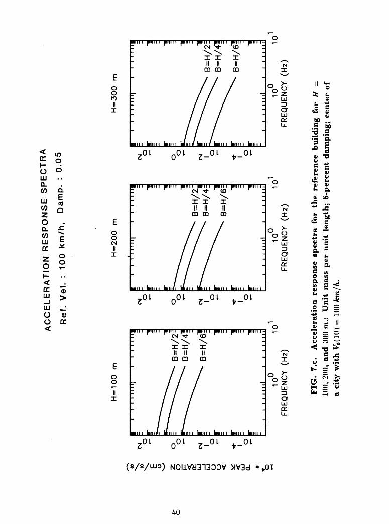
4 through 7. Figs. 4.a-c show the displacement spectra for 2-percent damping for for
V0 (10) = 50, 80, and 100 km/h, respectively, whereas Figs. 5.a-c show the same for 5-
percent damping. Corresponding curves for the acceleration spectra are given in Figs.
6.a-c and Figs. 7.a-c for 2-percent and 5-percent damping ratios. The spectra are plotted
on a log-log scale to be consistent with the convention used for earthquake excitations. As
the figures show, the displacement spectra are all straight lines. Recall that these spectra
are for the displacement due to dynamic wind forces only. The acceleration spectra differ
slightly from a straight line.
9. USE OF WIND TUNNELS FOR WIND RESPONSE SPECTRA
The wind response spectra in the previous section were developed by using an analyt
ical approach. A more accurate spectra can be developed in wind tunnels. The procedure
suggested here to develop spectra is based on a reference building, which is a rigid block
with rotational base spring and damper. This building can easily be modeled in a wind
tunnel by using a flexible base plate. By changing the flexibility of the base plate, the
response spectra can be obtained for a given location and a building with specified dimen
sions. By testing various buildings with different outside dimensions and damping ratios,
and also considering different wind conditions, a data base for wind response spectra can
be generated in the laboratory. It may be argued that modeling the roughness around the
building is an important and critical part of the wind tunnel tests, and it is unique for each
building. However, a generic roughness model for a given location can be approximated,
since wind spectra will be used for preliminary design purposes, rather than exact response
estimations.
22
10. COMFORT SPECTRA
Occupant discomfort due to wind-induced motions has long been recognized as one of
the major problems in high-rise buildings (Hansen, et. al., 1973). The discomfort is mainly
due to excessive low-frequency accelerations in the upper stories of buildings. The critical values of maximum acceleration for human comfort are available from experimental studies
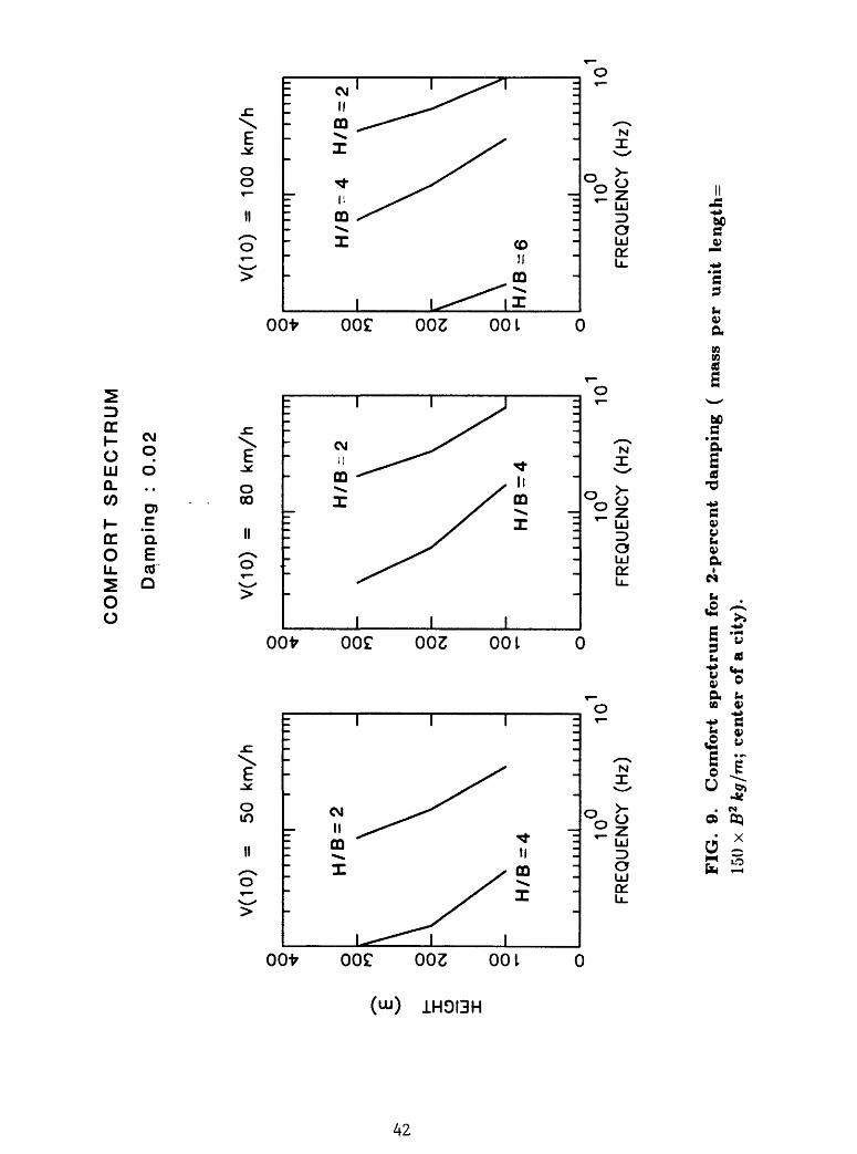
(NBCC, 1985). For a given building height and width, and wind structure, we can plot the acceleration response spectra. The intersection of the spectra with the straight line
representing the critical acceleration gives the critical frequency of the building. This is
schematically shown in Fig. 8. In order not to have human discomfort, the building should be designed to have a frequency higher than the critical frequency. If we determine critical frequency by using this approach for a range of building heights, we can then construct an interaction curve showing the building height versus critical frequency for a specifed
location. We will call this interaction curve the comfort spectrum. The left side of this curve (i.e., the lower frequency side) represents the uncomfortable side. We should select
building height and frequency to stay on the right side of the curve.
To give an .example, a set of comfort spectra for the reference building was developed
by considering the same set of values used for the development of response spectra in
section 8. To make the values realistic, we used m = 150. x B2 kg/m for the mass per unit
length instead of unit mass. The critical acceleration for human discomfort was taken as
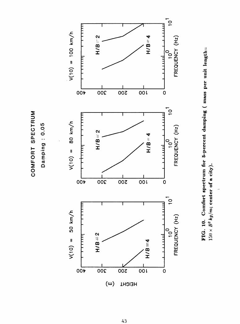
0.005g, where g is the gravitational acceleration. The comfort spectra are plotted in Fig.
9 for 2-percent damping, and in Fig. 10 for 5-percent damping. Each spectra is composed
of three points (corresponding to H =100, 200, and 300 m.), connected by straight lines.
11. JOINT DESIGN SPECTRA FOR WIND AND EARTHQUAKES
It is likely that for most buildings, either wind or earthquake will determine the design
criteria for lateral loads. Since we now can draw the wind response spectra in the same
way as the earthquake response spectra, we can easily plot them together superimposed on
the same axes, and see which one dominates at each frequency. This allows the designer
to determine which load is more critical for his building without doing any analysis.
An important drawback in this approach is that in any given location the probability of
occurence of a large storm is not equal to the probability of occurence of a large earthquake. Therefore, a straightforward comparison of the two spectra is not appropriate. We can
incorporate the probabilities of occurences in the spectra by using appropriate weighting
factors for each spectra, or we can scale each spectra in a probabilistic manner and compare
them for a specified exceedance (e.g., 90-percent) level.
We will investigate this topic in detail after we complete the second phase of the
23
study on wind spectra, where we will develop wind response spectra for across-wind vibra
tions. The reason for this is that for some buildings across-wind vibrations may dominate
the along-wind vibrations. In such cases we need to compare across-wind spectra with
earthquake spectra.
12. SUMMARY AND CONCLUSIONS
We have presented a response spectrum technique to estimate wind-induced dynamic
response (displacements and accelerations) of high-rise buildings. The method presented is
parallel to that used for earthquake excitations. At this phase of the research, we consider
only along-wind direction forces and vibrations. We will consider across-wind direction
response in the second phase of the research.
We develop wind response spectra for a reference building, defined as a single-degree-
of-freedom rectangular rigid block, with a rotational base spring and a damper. The wind
response spectrum is obtained as the peak response of the reference building for a range
of frequencies. We present 54 response spectra considering different combinations of wind
and structural configurations. We show that, for any given building, we can calculate peak
modal responses in terms of those of the reference building. We obtain the total peak
response of the building by combining peak modal responses.
We have also introduced the concept of comfort spectra. For a given building height,
we plot the acceleration response spectrum, and observe the building frequency corre
sponding to the critical acceleration for human discomfort. By doing this for a range of building heights, we can construct an interaction curve showing the building height versus
critical frequency. We call this interaction curve the comfort spectrum. We present a set
of examples for comfort spectra.
We conclude by discussing the development of a joint design spectrum for wind and
earthquakes loads. We will do a more detailed study on this topic after we complete
the second phase of the reserach, where we will develop response spectra for across-wind
vibrations.
24
REFERENCES
ANSI (1982). American National Standard, Minimum design loads for buildings and other structures, American National Standards Institute, Inc. , New York, NY, ANSI A58.1- 1982.
Cevallos-Candau, P.J. (1980). The commonality of earthquake and wind analysis, Ph.D. Thesis, Department of Civil Engineering, University of Illinois, Urbana, Illinois.
Davenport, A. G.(1961). The application of statistical concepts to the wind loading of structures, Proc., Inst. of Civil Eng., London, Vol. 19, pp. 449-472, 1961.
Davenport, A. G. (1964). The distribution of largest value of a random function with application to gust loading, Proc., Inst. of Civil Eng., London, Vol. 28, pp. 187-196, 1964.
Hansen, R.L., J.W. Reed, and E.H. Vanmarcke (1973). Human response to wind induced motion of buildings, Engineering Journal, American Institute of Steel Construction, July 1973.
Hurty, W.C. and M.F. Rubinstein (1964). Dynamics of Structures, Prentice-Hall, Inc., Englewood Cliffs, NJ.
Lin, Y. K. (1976). Probabilistic Theory of Structural Dynamics, Robert E. Krieger Pub lishing Company, Huntington, New York, 1976.
NBCC (1985). National Building Code of Canada, National Research Council of Canada, Ottawa, Canada.
Newmark, N.M. (1966). Relation between wind and earthquake response of tall buildings, proceedings, 1966 Illinois Structural Engineering Conference, University of Illinois, Urbana, 111.
Safak, E. and D.A. Foutch (1980). Vibration of buildings under random wind loads, Department of Civil Engineering, University of Illinois, SRS No. 480, Urbana, Illinois, May 1980.
§afak, E. and D.A. Foutch (1987). Coupled vibrations of rectangular buildings subjected to normally-incident random wind loads, Journal of Wind Engineering and Industrial Aero dynamics, 26, pp. 129-148.
Simiu, E. (1973). Logarithmic profiles and design wind speeds, Jour. of Eng. Mech. Div., ASCE, v.99, EM5, October 1973, pp.1073-1083.
Simiu, E. (1974). Wind spectra and dynamic alongwind response, Jour, of Struc. Div., ASCE, v.100, ST9, Sept. 1974, pp. 1877-1910.
Simiu, E. and R.H. Scanlan ( 1978). Wind Effects on Structures, an Introduction to Wind Engineering, John Wiley ana Sons, New York, 1978.
Vickery, B. J. (1971). On the reliability of gust loading factors, Civil Engineering Trans actions, pp. 1-9, April 1971.
25
VELOCITY
0
I9393a
cnC9** * 3
CTQ
3a<Jo" o>* **
*<J
M,
KoCo
yo(t)
y«(t)
FIG. 2. Single-degree-of-freedom damped oscillator subjected to base acceler ation.
27
T- Rigid block with unit / mass per unit height.
FIG. 3. Schematic view of the single-degree-of-freedom reference building used to generate response spectra.
28
104 * PEAK DISPLACEMENT (cm)
10~4 10~2 10° 102
* o2. - 0 «* a er £- OU d5 co sr ,_ o "Oo o I
Tj! I ot 3 0 d s * a B a 3. * t * n
? 3 29 t3 en A05 S
** CD
C «2. S
er(0
fi* n
I r 8 K&
5- »
m oc
XN
CD CD CDII II IIX XX
i tiiuf 11 HUB i IIIMJ iniiJ imiJ iniuJ i HIM
10"4 10~2 10° 102
m Oc
XN
GD CD CD II II II X XX X
-i mid i mud iniiJ iniiJ imiJ iniiJ iniiJ i HIM
10~4 10"2 10° 102
73m Oc
5°=
X N
_ CD CD CD. !! I! !!. X XX
k -IIHIIJ IIIIUJ lllllJ IIIIBJ IIIIMJ IIIIUJ IIHlJ I HIM
X II
Oo
3
X II
N3 O O
3
XII
O4o o
3
o
-o
< S <D rn - 2m
<» H O ^
TT ^3 m2. co 3- -0" O
3 m
m p ob HN) 30
DIS
PL
AC
EM
EN
T
RE
SP
ON
SE
S
PE
CT
RA
Ret.
Vel.
: 8Q
km
/h,
Da
mp
. :
0.0
2
H=
100
mH
=2
00
m
H=
300
m
E u UJ
LJ
O
CM O
O O
CM I O
O
I I
111
10°
FRE
QU
EN
CY
(H
z)10
CN O
O O
CM
I O
I T
T I
I
I II
I T
I IT
T1
B-H
/2J
B=
H/4
:
B=
H/6
itl 10°
10
FRE
QU
EN
CY
(H
z)
I I
I I
I I
I II
I I
I I
I M
l
10~
10
FR
EQ
UE
NC
Y
(Hz)
FIG
. 4.
b.
Dis
pla
cem
ent
resp
onse
sp
ectr
a fo
r th
e re
fere
nce
bu
ild
ing
for
H
100,
200
, an
d 3
00 m
.: U
nit
mas
s p
er u
nit
len
gth
; 2-
per
cen
t d
amp
ing;
cen
ter
of
a ci
ty w
ith
V0(
10)
= 8
0 k
m/h
.
DIS
PL
AC
EM
EN
T
RE
SP
ON
SE
S
PE
CT
RA
Ret.
Vel.
: 100
km
/h,
Dam
p.
: 0.0
2
H=
100
mH
=200
mH
=300
m
E u o 3 Q.
GO
O LJ
Q. * * O
(N O
O O
CM I O
I I
I I 1
11
B=
H/2
:
B=
H/4
~1
B=
H/6
l
10°
FRE
QU
EN
CY
(H
z)10
(N O
O O
CM I O
TT
T
10°
10
FREQUENCY (Hz)
10~
10
FREQUENCY (Hz)
FIG
. 4.
c.
Dis
pla
cem
ent
resp
onse
sp
ectr
a f
or t
he
refe
ren
ce
bu
ild
ing
for
H =
10
0, 2
00,
and
300
m.:
Un
it m
ass
per
un
it l
engt
h;
2-p
erce
nt
dam
pin
g; c
ente
r o
f a
city
wit
h F
0(10
) =
100
km
/h.
DIS
PL
AC
EM
EN
T
RE
SP
ON
SE
S
PE
CT
RA
Re
f.
Vel.
: 50
km
/h,
Dam
p.
: 0.0
5
H=
100
mH
=200
mH
=300
m
LJ
O 5 Q_
C/)
O
10
10
FRE
QU
EN
CY
(H
z)10
10
F
RE
QU
EN
CY
(H
z)
O O
04 I O
I I
I I
I IT
T|
I I
I I
I I If
B=
H/2
:
B=
H/4
l
B=
H/6
l
10°
10
FRE
QU
EN
CY
(H
z)
FIG
. 5.
a.
Dis
pla
cem
ent
resp
onse
sp
ectr
a fo
r th
e re
fere
nce
b
uil
din
g fo
r H
100,
200
, an
d 3
00 m
.:
Un
it m
ass
per
un
it l
engt
h;
5-p
erce
nt
dam
pin
g; c
ente
r of
a ci
ty w
ith
V0(
W)
= 5
0 k
m/h
.
DIS
PLA
CE
ME
NT
R
ES
PO
NS
E
SP
EC
TR
A
Ref.
Vel.
: 3
0
km
/h,
Dam
p.
: 0.0
5
H=
100
mH
=200
mH
=300
m
E o o Q.
Q 0. *
CN O O
CM
I O
i ill
10°
10
FR
EQ
UE
NC
Y
(Hz)
10°
FR
EQ
UE
NC
Y
(Hz)
10FR
EQ
UE
NC
Y
(Hz)
FIG
. 5.
b.
Dis
pla
cem
ent
resp
onse
sp
ectr
a f
or t
he
refe
ren
ce b
uil
din
g fo
r H
100,
200
, an
d 3
00 m
.:
Un
it m
ass
per
un
it l
engt
h;
5-p
erce
nt
dam
pin
g; c
ente
r o
f a
city
wit
h F
0(10
) =
80
km
/h.
104* PEAK DISPLACEMENT (cm)
*+ (B
|jLgH- O *O
2 ° 5TII .2 S- " 3§ d I
*
3 CO
g*Pj
« o en »S Q OJ» rt
11 CO
S o
s ->
"" 5T cn A i d 3- 7
5 = I I;
10 4 10 2 10°
73m Oc:
-
XN
I HIM I III
GO CD CDII II IIX XX
IIJ I I IIIJ
10-4
10-210'10'
m Oc
OO O
XN
". ITTHrillHB ITTT
CD CD CDII II IIX XX
k -tiuiJ i i HIM i mud IIIIHJ imuj iinuJ
10-4
10-2
10104
73m oc m
XN
CD CD CDII II IIX XX
itJ imuJ imJ i mud IIIIHJ imyj MIIUJ t mm
O O
XII 10 O O
O O
am W2, «
0 O. m
m o z /^ H
3 v.IT*
a0)313
mCO
COmCO
mo o b HOi 33
AC
CE
LE
RA
TIO
N
RE
SP
ON
SE
S
PE
CT
RA
Ref.
V
el.
:
50
km
/h,
Dam
p.
: 0
.02
H=
100
mH
=2
00
m
H=
300
m
CO \ E o a:
LJ
_j UJ o
o * o10
10
FR
EQ
UE
NC
Y
(Hz)
CM O
O O
CM I O
I I
I I
I I I
II
B=
H/2
E
B=
H/4
J
B=
H/6
J
10°
10
FRE
QU
EN
CY
(H
z)
CM O
O O
CM I O
III
IT T
U
I I
I 1I
I 10FR
EQ
UE
NC
Y
(Hz)
FIG
. 6.a
. A
ccel
era
tio
n
resp
on
se
spec
tra
fo
r th
e re
fere
nce
b
uil
din
g
for
H
=
100,
200
, an
d 3
00 m
.:
Un
it m
ass
per
un
it l
eng
th;
2-p
erce
nt
dam
pin
g;
cen
ter
of
a ci
ty w
ith
V0(
10)
= 5
0 k
m/h
.
104* PEAK ACCELERATION (cm/s/s)
» K "^a--5 s V*« IO
* 09 BT S
^«3S § 2.
10~4 10~2 10° 102
m Oc m _^
iiiuJ i mid iniuj mild iintJ i mud imiJ iin«
III
O O
3
GO «*£ C 5'
> 3 i a *001 Ow 3
"i en
g « 9 o
o ^
o ,2 « 5 3 «* oa «
I ? o c:5' ft en D
2 o* . *»
10~4 10~2 10° 102
m Ocz
X^k ^N
CD CD CD II II II XXX \ \\ ;
-IIIIUJ IIIIUJ IIIIUJ I I HUB IIIIMJ lllllJ IIIIUJ Mill
10~4 10"2 10° 102
m oc
XN
CD CD CD ii II ii XXX
CD -^ K) i miJ i miJ 1 1 HUB iinuJ i miJ iniuJ iniuJ i nm
XIIK)OO
3
XII
OJo o
3
33 O 0 O-*» mr-< m
H
oo O o z* 333 m ^ co? T>
O0 S 0) CO3 m
m o o
104* PEAK ACCELERATION (cm/s/s)
10~4 10~2 10° 102
-i 5 n ^ A j- . - Q10 '
arr- CL > " 2 t-1 cr 2o o JL - a «n 3 3^ " sr. § d o3
en 3 >0 S
8- 2 ^ 2 »3a
I I 1-1aq 3 oq
« O1 °
Oc
xNCO CO COII II II X XX
-imiW 11111 j i mm! i mini i mJi miij iniuj MUM
10~4 10~2 10° 102
~n
m o
IK'x'N
10~4 10~2 10° 102
70m Oc
XN
CO CO COII II II III \ \\
"iiiiiJ iiuiS i lima i iinJ 11 Hid i mid iintJ i HIM
X II
Oo
3
XIIN)OO
3
IIIGJ O O
3
2, m<(D
3 m* CO 3- "D
OO Z p CO3 m? CO"D
p S O H N> DO
ACCELERATION RESPONSE SPECTRA
Ref. Ve
l.
: 50 km
/h,
Damp.
: 0.05
H=
10
0
mH
=200
mH
=300
m
LO oo
w (0 E o Z O Sc O
O * o
CN
O
O O
CM
I O
Til
10°
10
FRE
QU
EN
CY
(H
z)
B=
H/2
1
B=
H/4
= T!
10
10
FR
EQ
UE
NC
Y
(Hz)
10~
10
FR
EQ
UE
NC
Y
(Hz)
FIG
. 7.
a.
Acc
eler
ati
on
re
spon
se
spec
tra f
or t
he
refe
ren
ce
bu
ild
ing
for
H
=
100,
200
, an
d 3
00 m
.:
Un
it m
ass
per
un
it l
engt
h;
5-p
erce
nt
dam
pin
g; c
ente
r o
f a
city
wit
h V
b(10
) =
50
km
/h.
6
104* PEAK ACCELERATION (cm/s/s)
1(T4 10~2 10° 102
9 H- 43
--s s
5T
^ °- >~ W 2 -' S 2 f~> O *» * * >- ~ 3 «ii E 3 00 «* c C 5* 5- s s 3 *