PROCESSING SYSTEMSChristoforos N. Hadjicostis,1 Hugo Rodrıguez Cortes,2
Aleksandar M. Stankovic2
1University of Cyprus and University of Illinois at Urbana-Champaign2Northeastern University
2.1 INTRODUCTION
Our main research goal was to develop a comprehensive framework for faulttolerance enhancement in electric drives and power systems. This framework wasto serve as a general tool for analysis and fault-tolerant operation. Its developmentled us to re-examine the foundations of fault detection and accommodation inenergy-processing systems.
Energy processing systems share a number of features with other large, complexengineered systems, including the possibility of failure of components and links.Present technology tends to emphasize the role of automation in detecting andaccommodating equipment failures and in maintaining system integrity. In powersystems the problem of component failure is addressed in the framework ofsecurity. The main premise is that the analyst can generate a list of likely (credible)outages, and then study the effects of each of these outages using the best availableinformation about the state of the system at the time of interest. In utility practicethe list of outages typically includes faults of major (single) pieces of equipment,
like generators, transmission lines, loads, and transformers. Under the assumptionthat the system protection correctly identifies the faulted piece, a static (load-flow)analysis is performed on the remaining system (with the faulted piece disconnected)to ensure that the system continues to operate within acceptable performance andsafety limits. The models used in the process often come from system design studies,and they have not been verified by specific experiments. The US Navy uses a similarprocedure: the damage tolerance analysis includes a generation of the list of failedcomponents (often as a part of weapons damage assessment), followed by a staticanalysis of line flows and node voltages.
Neither utility nor Navy experts are completely satisfied with the present stateof affairs. Months of studies and model tuning are often necessary to only qualita-tively capture the main features of systemwide outages, such as in California in 1996.Improvements that have been considered (mostly in the research literature) include theuse of dynamical models for assessment of prefault states (dynamic state estimation)and of transients following the outage (the so-called dynamic security assessment).Two main stumbling blocks with this approach are the need to tailor the level ofdetail for component models (so as to keep the overall model tractable) and the needto include the effects (and possible misfiring) of protection in a systematic fashion.
In our research we developed dynamic models for various tasks, including com-ponent protection, dynamic fault detection, and accommodation, and made novelconnections with traditional fault detection techniques. Toward this end, in Section 1.2we review model-based fault detection techniques. The review covers failure detectionfiltering approaches, starting from the pioneering work of Beard and Jones and endingat the detection schemes based on differential geometry techniques. The rest of thechapter is devoted to the solution of fault detection problems in energy processingsystems. We begin in Section 1.3 with a monitoring scheme to detect detuned opera-tion in IFOC driven induction motors. In Section 1.3 we propose a monitoring schemeto detect broken rotor bars on IFOC-driven squirrel cage induction motors. Finally, inSection 1.5 we propose a monitoring scheme to detect bus load changes, symmetricline short circuits, and lost lines on the power system of the Navy electric ship.
2.2 MODEL-BASED FAULT DETECTION
The basic function of a fault detection scheme is to produce an alarm when a faultoccurs in the monitored system, and in a second stage to identify the failed component.Ideally the alarm should be a binary signal announcing that a fault is influencing thesystem or that no fault is hampering the system. Another important characteristic forthe alarm is the speed of detection. It is desirable to have a fault detection schemethat produces an alarm immediately after the occurrence of the fault. Finally, themost important characteristic of the alarm is the rate of false alarms, as false alarmsdeteriorate the performance of fault detection schemes. Thus a great effort in thedesign of fault detection schemes focuses on the problem of generation of alarmsproviding effective discrimination between different faults, system disturbances andmodeling uncertainties.
MODEL-BASED FAULT DETECTION 17
2.2.1 Fault Detection via Analytic Redundancy
Residuals, also denoted as alarms, are quantities expressing the difference between theactual plant outputs and those expected on the basis of the applied inputs and the math-ematical model. They are obtained by exploiting dynamic or static relationships amongsensor outputs and actuator inputs. An important characteristic for residuals is that theyneed to be robust with respect to the effect of nuisance faults; otherwise, nuisancefaults will obscure the residual’s performance by acting as a source of false alarms.
The general procedure of fault detection, isolation and accommodation (FDIA)in dynamic systems with the aid of analytical redundancy consists of the followingthree steps [20]:
1. Generation of functions that carry information about the faults, so-called resid-uals.
2. Decision about the occurrence of a fault and localization of the fault, so-calledisolation.
3. Accommodation of the faulty process, and transition to normal operation.
To date, much of the work on the generation of residuals mostly performed within theanalytic redundancy framework observes two important tendencies: failure detectionfilters and parity relations. The similarities between these two approaches lead to thesame residuals being applicable for linear systems and for some nonlinear systems [8].
2.2.2 Failure Detection Filters
Beard [2] was the first to propose a fault detection filter, refined later by Jones [10]. Inthis filter, known as the Beard–Jones detection (BJD) filter, the reachable subspacesof each fault are placed into invariant independent subspaces. Then, when a nonzeroresidual is detected, the fault is identified by projecting the residual onto the reachablesubspaces of faults and comparing the projection against a threshold. Even thoughmultiple faults can be detected with this filter, the approach is very restrictive asfaults have to satisfy a mutual detectability condition [15].
Further improvements to the BJD filter were suggested in [16] with the restricteddiagonal detection (RDD) filter. In this approach faults are divided into faults thatneed to be detected (so-called target faults) and nuisance faults (e.g., parameter uncer-tainties, changes in system parameters, and noise). Nuisance faults are projected ontothe unobservable space of residuals while maintaining observability of target faults;then target faults are identified as in the BJD filter. When every fault is detected, BJDand RDD filters are equivalent.
The most recent version of the BJD filter, the so-called unknown input (UI)observer approach, was proposed in [20] using the eigenstructure assignment and theKronecker canonical form as design methods, and in [16] using geometric techniques.In the UI observer approach, nuisance faults are projected onto the unobservablesubspace so that residuals are influenced only by the target fault, simplifying in thisway the decision task. It should be pointed out that even though the use of UI observers
18 DYNAMICAL MODELS IN FAULT-TOLERANT OPERATION
in fault detection and isolation was first proposed in [16–20], UI observers havereceived significant attention only after the pioneering work of Basille and Marro,presented for instance in [1]. In this chapter we consider the UI observer approachwith geometric techniques.
In the nonlinear setting, the residual generation problem using analytic redundancyhas been addressed in [9] for state-affine systems and lately in [6] for input-affinesystems. In these works residual generator construction is based, under some mildadditional assumptions, on the existence of an unobservability subspace (distribution)leading to a subsystem unaffected by all fault signals but the fault of interest; then anasymptotic observer for such a subsystem, which in the nonlinear case may not exist,yields the residual generator.
Consider the nonlinear system
x = f (x) + g(x)u + lN (x)mN + lT (x)mT
y = h(x)(2.1)
where x ∈ Rn is the state, y ∈ Rk is the measurable output, mN ∈ Rl1 and mT ∈ Rl2
are arbitrary functions of time representing the nuisance and target failure modesrespectively. During fault free operation the failure modes are equal to zero. Thecolumns of f (x), g(x), h(x), lT (x), and lT (x) are smooth vector fields. The matriceslT (x) and lN (x) denote the failure signatures.
Problem 1: Consider the energy processing system described by equation (2.1)Design a dynamic residual generator with state x ∈ Re , of the form
˙x = F (x , y) + E (x , y)ur = M (x , y)
(2.2)
where F (x , y), E (x , y), and M (x , y) are smooth vector fields, that takes y and u asinputs and generates the residual signal r with the following local properties:
I. When the target failure is not present, r decays asymptotically to zero; thatis, the transmission from u and nuisance faults is zero and r is asymptoticallystable.
II. For a nonzero target fault, the residual is nonzero.
Condition I considers the stability of the residual generator and ensures that the inputsignal u and the nuisance faults mN do not affect the residual r . Condition II guaranteesthat the target fault affects the residual.
In [6] a necessary condition for the existence of a solution to Problem 1 is given.This condition, under some mild assumptions, leads to a subsystem driven only bythe fault of interest. Thus the solution to Problem 1 can be found provided there is anobserver for such a subsystem. Specifically, assume that the minimal unobservabilitydistribution of (2.1), denoted by S ∗, that contains the image of the nuisance faultsignature is locally nonsingular. Then it can be shown that if
S ∗ ∩ span{lT(x)} = {0} (2.3)
DETUNING DETECTION AND ACCOMMODATION ON IFOC-DRIVEN INDUCTION MOTORS 19
it is possible to find a state diffeomorphism and an output diffeomorphism⎡⎣z1
z2
z3
⎤⎦ = φ(x),
[w1
w2
]= ψ(y) (2.4)
such that in the new coordinates the system (2.1) is described by equations of theform
z1 = f1(z1, z2) + g1(z1, z2) + lT 1(z )mT
z2 = f2(z ) + g2(z ) + lN 2(z )mN + LT 2(z )mT
z3 = f3(z ) + g3(z ) + lN 3(z )mN + LT 3(z )mT
w1 = h1(z1)
w2 = z2
From these equations it is possible to extract a subsystem driven only by the fault ofinterest (target fault) as
z1 = f1(z1, z2) + g1(z1, z2) + lT 1(z )mT
w1 = h1(z1)(2.5)
Clearly, when it is possible to design an observer for (2.5), the residual generationproblem is solvable. The minimal unobservability distribution S ∗ containing the imageof the nuisance fault signature can be computed as the last element of the sequence
S0 = W ∗ + Ker{dh}Sk = W ∗ + [ f , Sk−1 ∩ Ker{dh}] + [ g , Sk−1 ∩ Ker{dh}], i = 1, . . . , k
(2.6)
where k ≤ n − 1 is determined by the condition Sk = Sk−1. Concerning W ∗, it iscomputed as the last element of the following sequence:
W0 = PWi = W i−1 + [ f , W i−1 ∩ Ker{dh}] + [ g , W i−1 ∩ Ker dh], i = 1, . . . , k
(2.7)
with i ≤ n − 1 determined by the condition Wi+1 = Wi . In (2.6) and (2.7) the [. , .]denotes the Lie product, X denotes the involutive closure of X , and P = span{lN (x)}.
Finally, we consider nonlinear systems with unstructured failure modes describedby equations of the form
x = f (x , mT , mN ) + g(x , mT , mN )uy = h(x)
(2.8)
2.3 DETUNING DETECTION AND ACCOMMODATIONON IFOC-DRIVEN INDUCTION MOTORS
In most high-performance applications of electric drives (e.g., speed and positionservos), the control structure utilized is the so-called field oriented (vector) control.It allows for (almost) decoupled control of torque and flux, and yields a very fast
20 DYNAMICAL MODELS IN FAULT-TOLERANT OPERATION
transient response. In the case of a well-tuned controller, the main performance limi-tations come from the current bandwidth of the drive. With modern power electronicswitching devices (e.g., IGBT) that bandwidth is well above a kHz, resulting in out-standing electromechanical response. In the case of a detuned operation, however, theperformance can degrade substantially, both in transients (torque command following)and in steady state (efficiency). If the detuning is caused by a typically nonmonitoredprocess (e.g., rotor time constant variation, or a slow degradation of the shaft positionsensor information), it may go undetected for a while, and lead to drastic efficiencyreduction, or even a hard fault. In this chapter we propose model-based scheme todetect the detuning process in a general purpose field-oriented induction drive motor.It is based on differential geometric considerations, and it is immune to a number oftransients that normally occur in a high-performance drive, like load torque variations.
2.3.1 Detuned Operation of Current-Fed Indirect Field-OrientedControlled Induction Motors
It is well known that mechanical commutation simplifies significantly the control taskin DC motors. The action of the commutator is to reverse the direction of the armaturewinding currents as the coils pass the brush position so that the armature currentdistribution is fixed in space regardless of the rotor speed. Thus the field flux producedby the stator and the magneto-motive force (MMF) created by the current in thearmature winding are maintained in a mutually perpendicular orientation independentof the rotor speed. The result of this orthogonality is that the field flux is practicallyunaffected by the armature current, as a result when the field flux is kept constant,the produced electromechanical torque is proportional to the armature current. Highdynamic performance can be obtained using two linear control loops, one (slow)controlling the field flux and the other (fast) one controlling the armature current.
In induction motors field flux and armature MMF distributions are not orthogonal,rendering the analysis and control of these devices more complicated. However, theaction of the commutator of a DC machine in holding a fixed orthogonal spatialangle between the field flux and the armature MMF can be emulated in inductionmachines by orienting the stator current with respect to the rotor flux so as to attainpractically independent controlled flux and torque. Such controllers are called field-oriented controllers and they require independent control of both magnitude and phaseof the AC quantities.
An understanding of the decoupled flux and torque control resulting from fieldorientation can be attained from the model of an induction machine in the fixed statorframe [13,18,19]
σd
dtiαs = −
(rs + Lm
Lrτr
)iαs + ωr
Lm
Lrλβr + Lm
Lrτrλαr + vαs
σd
dtiβs = −
(rs + Lm
Lrτr
)iβs − ωr
Lm
Lrλαr + Lm
Lrτrλβr + vβs
d
dtλαr = − 1
τrλαr − ωrλβr + Lm
τriαs (2.9)
DETUNING DETECTION AND ACCOMMODATION ON IFOC-DRIVEN INDUCTION MOTORS 21
d
dtλβr = − 1
τrλβr + ωrλαr + Lm
τriβs
2J
P
d
dtωr = P
2
Lm
Lr(λαr iβs − λβr iαs) − τL
where iαβs are the stator currents, λαβr are the rotor flux linkages, vαβs are the sta-tor voltages, ωr (P/2) is the mechanical velocity, P is the number of poles in themachine, J is the rotational inertia, τL is the torque load, rs , rr are the stator androtor resistances, Ls , Lr , Lm are the stator, rotor and mutual inductances, τr = Lr/rr
and σ = Ls − L2m/Lr .
The field orientation concept implies that the current components supplied to themachine should be oriented in phase (flux components) and in quadrature (torquecomponent) to the rotor flux vector λαβr . This can be accomplished by choosing ωe
to be the instantaneous speed of λαβr and locking the phase of the reference systemto the direction of the magnetizing flux λM ; that is,[
λM
0
]= e−J θe
[λαr
λβr
](2.10)
where
eJ θe =[
cos(x) − sin(θe)
sin(x) cos(x)
].
When the machine is supplied from a current-regulated source, the stator equationscan be omitted; the rotor dynamics, in terms of stator currents and rotor flux, in arotor field-oriented frame is described by the equations
d
dtλM = − 1
τrλM + Lm
τrids (2.11)
ωe = ωr + Lm
τr
iβs
λM(2.12)
2J
P
d
dtωr = P
2
Lm
LrλM iqs − τL (2.13)
with idqs = e−J θe iαβs
Equations (2.11) to (2.13) describe the dynamic response of a field-oriented induc-tion machine and essentially parallel the DC machine dynamics. Equation (2.11)corresponds to the field circuit on a DC machine. Equation (2.12) defines what iscommonly called the slip frequency ωs = ωe − ωr which is inherently associated withthe division of the input stator current into the desired flux and torque components.The electromechanical torque in (2.13) shows the desired torque control property ofproviding a torque proportional to the torque command current iqs .
The implementation of field orientation can be easily carried out provided thatthe position angle of the rotor flux θe is known. There are two basic approaches todetermine θe : direct schemes, which determine the angle from flux measurements, and
22 DYNAMICAL MODELS IN FAULT-TOLERANT OPERATION
SPEEDREGULATOR
INDUCTION MOTOR
IFOC dq2ab
ab2dq
i abs
i *qs
i *ds
v abs
v dqs
i dqs
CURRENTREGULATOR
wr
w*r
∧
q e∧
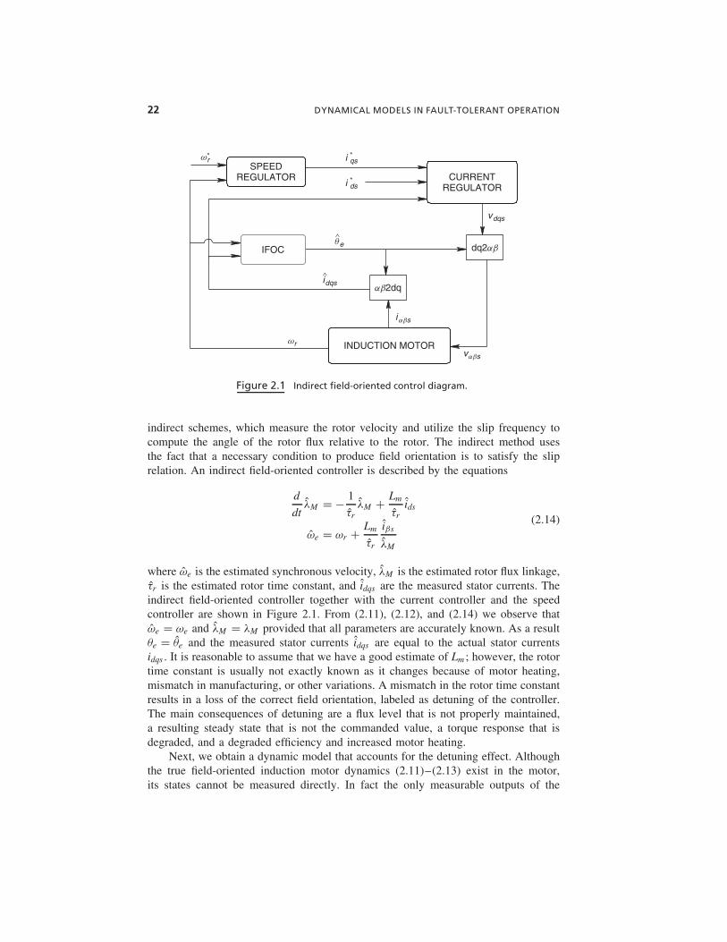
Figure 2.1 Indirect field-oriented control diagram.
indirect schemes, which measure the rotor velocity and utilize the slip frequency tocompute the angle of the rotor flux relative to the rotor. The indirect method usesthe fact that a necessary condition to produce field orientation is to satisfy the sliprelation. An indirect field-oriented controller is described by the equations
d
dtλM = − 1
τrλM + Lm
τrids
ωe = ωr + Lm
τr
iβs
λM
(2.14)
where ωe is the estimated synchronous velocity, λM is the estimated rotor flux linkage,τr is the estimated rotor time constant, and idqs are the measured stator currents. Theindirect field-oriented controller together with the current controller and the speedcontroller are shown in Figure 2.1. From (2.11), (2.12), and (2.14) we observe thatωe = ωe and λM = λM provided that all parameters are accurately known. As a resultθe = θe and the measured stator currents idqs are equal to the actual stator currentsidqs . It is reasonable to assume that we have a good estimate of Lm ; however, the rotortime constant is usually not exactly known as it changes because of motor heating,mismatch in manufacturing, or other variations. A mismatch in the rotor time constantresults in a loss of the correct field orientation, labeled as detuning of the controller.The main consequences of detuning are a flux level that is not properly maintained,a resulting steady state that is not the commanded value, a torque response that isdegraded, and a degraded efficiency and increased motor heating.
Next, we obtain a dynamic model that accounts for the detuning effect. Althoughthe true field-oriented induction motor dynamics (2.11)–(2.13) exist in the motor,its states cannot be measured directly. In fact the only measurable outputs of the
DETUNING DETECTION AND ACCOMMODATION ON IFOC-DRIVEN INDUCTION MOTORS 23
qs
qs
bs
as
qe
qe
∧
ds
ds
∧
∧
Figure 2.2 Fixed frame and rotating frames.
induction motor are the stator currents in the abc frame and the mechanical rotorspeed ωr . Since it is assumed that the induction motor is wye connected, the currentsiαβs can be obtained from iabcs as follows:
iαs =√
3
2ias
iβs = 1√2(ibs − ics )
(2.15)
As observed in Figure 2.2, the relation between currents iαβs and currents idqs isdefined by
iαβs = eJ θe idqs (2.16)
Note now that in a detuned condition (θe �= θe) stator currents are given as
idqs = e−J θe iαβs (2.17)
thus from (1.16) and (1.17) we conclude that
idqs = e−J θe idqs (2.18)
with θe = θe − θe .Replacing (2.18) into (2.11) to (2.13) and reordering terms, we get an indirect
field-oriented controlled induction motor model that includes detuning effects and isdescribed by the following equations:
d
dtλM = − 1
τrλM + Lm
τr
[cos(θe)ids + sin(θe)iqs
]d
dtθe = Lm
τr
cos(θe)iqs − sin(θe)ids
λM− Lm
τr
ids
λM
24 DYNAMICAL MODELS IN FAULT-TOLERANT OPERATION
d
dtλM = − 1
τrλM + Lm
τrids (2.19)
2J
P
d
dtωr = P
2
Lm
LrλM
[cos(θe)iqs − sin(θe)ids
]− τL
where ddt θe = ωe − ωe . Note now that in steady state, from equation (2.19) we have
that
1
τr
cos(θe)iqs − sin(θe)ids
cos(θe)ids + sin(θe)iqs= 1
τr
iqs
ids(2.20)
This gives
tan(θe) =(
1 − τrτr
)iqs
ids
1 + τrτr
(iqs
ids
)2
thus θe = 0 provided that τr = τr .
2.3.2 Detection of the Detuned Operation
Next we design a residual generator to detect detuned indirect field-oriented controllersfollowing the model-based fault detection method outlined in the previous section.We consider θe in (2.19) as an externally generated signal, and for fault detection weconsider the following system:
d
dtλM = − 1
τrλM + Lm
τr[cos(θe)ids + sin(θe)iqs ]
2J
P
d
dtωr = P
2
Lm
LrλM [cos(θe)iqs − sin(θe)ids ] − τL
(2.21)
Note now that to express the dynamics in (2.21) in terms of the system (2.1), we needto identify the target and nuisance faults. Since the load torque τL is also an unknownquantity that may vary over a wide range depending on the motor application, weconsider it as a nuisance fault; that is,
lN =[
0
− P
2J
]
Note that now the information about detuning (θe �= 0) is contained on the trigono-metric functions of (2.21). So, by defining,
mT =[
cos(θe) − 1sin(θe)
]
DETUNING DETECTION AND ACCOMMODATION ON IFOC-DRIVEN INDUCTION MOTORS 25
we have
lT =
⎡⎢⎣
Lm
τrids
Lm
τriqs
P2
4J
Lm
LrλM iqs −P2
4J
Lm
LrλM ids
⎤⎥⎦ ,
f =⎡⎣− 1
τrλM
0
⎤⎦ , g =
⎡⎢⎣
Lm
τr0
0P2
4J
Lm
LrλM
⎤⎥⎦
and u = [ids iqs ].As was stated previously, the only measurable quantity in (2.21) is the rotor speed
ωr ; that is,
y = ωr (2.22)
Straightforward computations show that for (2.22) the minimal unobservability distri-bution is given as
S ∗ωr
= span
⎧⎪⎨⎪⎩
01
τr
− P
2J0
⎫⎪⎬⎪⎭
and condition (2.3) is not satisfied.Consider further the magnetizing flux as the output of the system:
y1 = λM (2.23)
Analogous computations show that
S ∗λM
= span
{0
− P
2J
}
and condition (2.3) is satisfied.By inspection we see that in this case the subsystem (2.5), with z1 = λM and
w1 = y1, reads as
λM = − 1
τrλM + Lm
τrids + Lm
τrids mt1 + Lm
τriqs mt2
Hence we have a solution to Problem 1 by designing an observer for subsystem (2.24).Note that in (2.24) the rotor time constant is unknown. However, the residual generator
λM = − 1
τrλM + Lm
τrids − �(λM − λM )
r = λM − λM
(2.24)
where � > 0 solves Problem 1.
26 DYNAMICAL MODELS IN FAULT-TOLERANT OPERATION
To verify that a solution to Problem 1 is given by (2.24), note that the dynamicsof the residual is described by the equation
r = −�r −(
1
τr− 1
τr
)(λM − Lm ids) − Lm
τrids mt1 − Lm
τriqs mt2 (2.25)
The second right-hand term in (2.25) is somewhat unexpected; however, we noticethat this term will be zero provided mt1 and mt2 are equal to zero. This term, in fact,also represents the detuning problem expressed as the difference between the estimatedrotor time constant and the actual rotor time constant. Hence we have established that(2.24) is a solution to Problem 1.
2.3.3 Estimation of the Magnetizing Flux
Note that to compute the residual, we need to have access to the magnetizing fluxλM , which is not typically available. As stated in [17], this flux can be computed asfollows. Assuming that the rotor dynamics is in steady state, we have
σ
[iβs
d
dtiαs − iαs
d
dtiβs
]= ωe
Lrλ2
M + q (2.26)
where q = vαs iβs − vβs iαs . Define now
θ = arctan
(iαs
iβs
)(2.27)
thus (2.26) can be written as
θ =ωeLr
λ2M + q
σ(i 2αs + i 2
βs)(2.28)
Under the assumption above λM is a constant in (2.28). In order to estimate λM , wefollow the general results presented in [11]. Define the estimation error
z = � − λ2M + β(θ) (2.29)
thus we have
z = � + ∂β
∂θ
ωeLr
(� − z + β(θ)) + q
σ(i 2αs + i 2
βs)
Defining
β(θ) = K σθ , � = −KωeLr
(� − z + β(θ)) + q
σ(i 2αs + i 2
βs)(2.30)
DETUNING DETECTION AND ACCOMMODATION ON IFOC-DRIVEN INDUCTION MOTORS 27
with K > 0, we can describe the estimation error dynamics by
z = − K
Lr
ωe
(i 2αs + i 2
βs )z
thus z converges exponentially to zero and
limt→∞(� − λ2
M + K σθ) = 0 (2.31)
Finally, from (2.31) we have that
λM =√
|� + K σθ |We can also estimate the magnetizing flux from stator steady state values. To see this,note that
iβsd
dtiαs − iαs
d
dtiβs = iqs
d
dtids − ids
d
dtiqs − ωe[i 2
αs + i 2βs ] (2.32)
Thus, by replacing (2.32) into (2.26) and assuming that the stator dynamics is insteady state, we have
λM =√∣∣∣∣ Lr
ωe(vβs iαs − vαs iβs ) − σLr (i 2
αs + i 2βs)
∣∣∣∣2.3.4 Accommodation of the Detuning Operation
In steady state we have
ids = λM
Lm
Moreover, since (2.18) implies
‖idqs‖ = ‖idqs‖we can compute iqs as
iqs =√
i 2ds + i 2
qs + i 2ds (2.33)
Finally, from (1.20) we have
τr = τriqs
ids
ids
iqs(2.34)
For accommodation of the detuning operation, we define a threshold rm > 0 for theresidual in such a way that the IFOC is detuned provided that |r |> rm . This thresholdreduces the effect of noise and other nonmodeled dynamics on the decision.
Once it is decided that the IFOC is detuned, the accommodation procedure waitsfor the system to achieve a steady state operation. Then it computes the new rotortime constant from (1.34), and sends it to the IFOC scheme.
28 DYNAMICAL MODELS IN FAULT-TOLERANT OPERATION
TABLE 2.1 Parameters of the induction motor
Parameter Motor (3 HP)
Ls , Lr (H ) 0.3826,0.3808Lm(H ) 0.3687rr , rs (�) 1.34, 1.77P 4
Time (s)
Res
idua
l r
0−0.5
0.5
−0.25
0
0.25
3 6 11 17 20
Rot
or ti
me
cons
tant
tr
0.8
0.5684
0.2842
0.1421
0
Time (s)
0 3 6 11 17 20
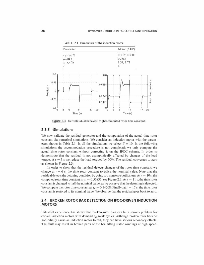
Figure 2.3 (Left) Residual behavior; (right) computed rotor time constant.
2.3.5 Simulations
We now validate the residual generator and the computation of the actual time rotorconstant via numerical simulations. We consider an induction motor with the param-eters shown in Table 2.1. In all the simulations we select � = 10. In the followingsimulations the accommodation procedure is not completed; we only compute theactual time rotor constant without correcting it on the IFOC scheme. In order todemonstrate that the residual is not asymptotically affected by changes of the loadtorque, at t = 3 s we reduce the load torqued by 50%. The residual converges to zeroas shown in Figure 2.3.
In order to show that the residual detects changes of the rotor time constant, wechange at t = 6 s, the time rotor constant to twice the nominal value. Note that theresidual detects the detuning condition by going to a nonzero equilibrium. At t = 10 s, thecomputed rotor time constant is τr = 0.56836; see Figure 2.3. At t = 11 s, the time rotorconstant is changed to half the nominal value, as we observe that the detuning is detected.We compute the rotor time constant as τr = 0.14208. Finally, at t = 17 s, the time rotorconstant is restored to its nominal value. We observe that the residual goes back to zero.
2.4 BROKEN ROTOR BAR DETECTION ON IFOC-DRIVEN INDUCTIONMOTORS
Industrial experience has shown that broken rotor bars can be a serious problem forcertain induction motors with demanding work cycles. Although broken rotor bars donot initially cause an induction motor to fail, they can have serious secondary effects.The fault may result in broken parts of the bar hitting stator windings at high speed.
BROKEN ROTOR BAR DETECTION ON IFOC-DRIVEN INDUCTION MOTORS 29
This in turn can cause a serious damage to the induction motor; therefore faulty rotorbars need to be detected as early as possible.
Broken rotor bars cause disturbances of the flux pattern in induction machines.These non-uniform magnetic field components influence machine torque and statorterminal quantities, and are thus detectable, in principle, by monitoring schemes.To date, different methods have been proposed for broken rotor bar detection. Themost well known approach is the non–model-based motor current signature analysis(MCSA) method [26]. This method monitors the spectrum of a single phase ofthe stator current for frequency components associated with broken rotor bars. Themain disadvantage of the MCSA method is that it relies on the interpretation ofthe frequency components of the stator current spectrum that are influenced bymany factors, including variations in electric supply and in static and dynamic loadconditions. These conditions can lead to errors in the fault detection task [3]. Onthe other hand, a practical advantage of MCSA is that only stator currents needto be measured. Efforts to eliminate the influence of load conditions have beenpresented, for instance, in [24] where it is shown that the direct component of thestator currents in a synchronous frame is not affected by load conditions; thus it isproposed to monitor the spectrum of that stator current component. It turns out thatin our proposed monitoring scheme we monitor a state closely related to the directcomponent of the stator current. However, we discovered our signal selection usinggeometric techniques. Fuzzy logic [22] and neural network [7] techniques have beenalso proposed to handle load-related ambiguous frequency components. The MCSAmethod has been the main approach used for detecting broken rotor bars on inductionmotors operating in open-loop. However, spectral analysis techniques applicable undervariable speed conditions have also been presented in the literature (e. g., [4,27]).
Despite the extensive work on broken rotor bar detection, model-based techniqueshave not received much attention. Main reasons are that fault-related induction motorparameters are not well known, and available models are quite complicated to betractable with model-based fault detection techniques. However, by making a compro-mise between a better tracking of the fault-related signals (by using dynamic models)and a reduced domain of applicability of the results (due to assumptions about theinduction motor parameters), model-based broken rotor bar detection techniques havebeen recently proposed. One such example is the Vienna monitoring method (VMM)presented in [12]. The VMM is based on the comparison of the computed electrome-chanical torque from two real-time machine models. A healthy induction motor leadsto equal values computed by the two models, whereas a faulted induction motor excitesthe models in a different way, leading to a difference between computed torque values.This difference is used to determine the existence of broken rotor bars. The VMM hasone disadvantage, which is also present in our proposed monitoring scheme: variationson the time rotor constant deteriorate the performance of the fault detection scheme.
2.4.1 Squirrel Cage Induction Motor Model with Broken RotorBars
We present now an induction motor model with broken rotor bars. The proposedmodel is less detailed than the models presented, for instance, in [14] and [29]. Anovel feature is that the effect of broken rotor bars is taken into account by adding only
30 DYNAMICAL MODELS IN FAULT-TOLERANT OPERATION
a s′c s′
b b′ b b
g
b s′as
cs
cr
as
ar
bs
br
cs bs
a r′c r′ b r′ar cr br
2π π
fr
fs
qr
a
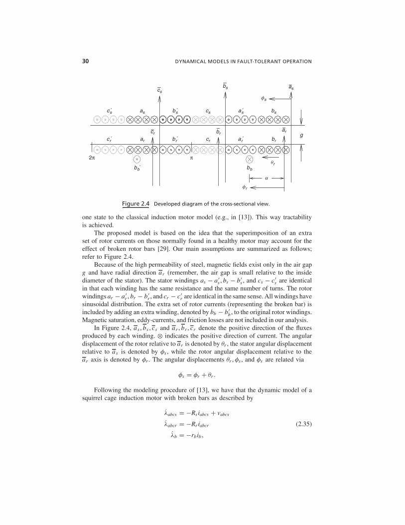
Figure 2.4 Developed diagram of the cross-sectional view.
one state to the classical induction motor model (e.g., in [13]). This way tractabilityis achieved.
The proposed model is based on the idea that the superimposition of an extraset of rotor currents on those normally found in a healthy motor may account for theeffect of broken rotor bars [29]. Our main assumptions are summarized as follows;refer to Figure 2.4.
Because of the high permeability of steel, magnetic fields exist only in the air gapg and have radial direction ar (remember, the air gap is small relative to the insidediameter of the stator). The stator windings as − a ′
s , bs − b ′s , and cs − c′
s are identicalin that each winding has the same resistance and the same number of turns. The rotorwindings ar − a ′
r , br − b ′r , and cr − c′
r are identical in the same sense. All windings havesinusoidal distribution. The extra set of rotor currents (representing the broken bar) isincluded by adding an extra winding, denoted by bb − b ′
b , to the original rotor windings.Magnetic saturation, eddy-currents, and friction losses are not included in our analysis.
In Figure 2.4, as , bs , cs and ar , br , cr denote the positive direction of the fluxesproduced by each winding. ⊗ indicates the positive direction of current. The angulardisplacement of the rotor relative to ar is denoted by θr , the stator angular displacementrelative to as is denoted by φs , while the rotor angular displacement relative to thear axis is denoted by φr . The angular displacements θr , φs , and φs are related via
φs = φr + θr .
Following the modeling procedure of [13], we have that the dynamic model of asquirrel cage induction motor with broken bars as described by
λabcs = −Rs iabcs + vabcs
λabcr = −Rr iabcr (2.35)
λb = −rbib ,
BROKEN ROTOR BAR DETECTION ON IFOC-DRIVEN INDUCTION MOTORS 31
where λabcs , λabcr are the stator and rotor flux linkages, iabcs , iabcr are the stator androtor currents, vabcs is the stator voltage, λb , ib are the broken bar flux linkage andcurrent, Rr = diag{rr } is the rotor resistance, and Rs = diag{rs} is the stator resistance.Flux linkages and currents are related as
⎡⎣iabcs
iabcr
ib
⎤⎦ =
⎡⎣ Ls Lsr Lbs
LTsr Lr Lbr
LTbs LT
br Lb
⎤⎦
−1 ⎡⎣λabcs
λabcr
λb
⎤⎦ (2.36)
where
Lbs = −Lbs
[cos(α)cos
(α − 2π
3
)cos
(α + 2π
3
)]
Lbr = −Lbr
[cos(θr − α)cos
(θr − α − 2π
3
)cos
(θr − α + 2π
3
)]
Ls =
⎡⎢⎢⎢⎢⎣
Lls + Lms −Lms
2−Lms
2−Lms
2Lls + Lms −Lms
2−Lms
2−Lms
2Lls + Lms
⎤⎥⎥⎥⎥⎦ (2.37)
Lsr = Lsr
⎡⎢⎢⎢⎢⎢⎢⎣
cos(θr ) cos
(θr + 2π
3
)cos
(θr − 2π
3
)
cos
(θr − 2π
3
)cos(θr ) cos
(θr + 2π
3
)
cos
(θr + 2π
3
)cos
(θr − 2π
3
)cos(θr )
⎤⎥⎥⎥⎥⎥⎥⎦
In equations (2.36) and (2.37), Lls , Lms are the stator leakage and self inductance,Llr , Lmr are the rotor leakage and self-inductance, Lsr = Lms is the stator–rotor mutualinductance, Lbr , Lbs = Lbr are the broken bar–stator and broken bar–rotor mutualinductance, respectively, Lb is the broken bar self-inductance, and α is the angularposition of the broken bar. Finally, the mechanical dynamics is described by
J ωm = P
2
d
dθr
(i Tabcs Lsr iabcr + i T
abcs Lbs ibb) − τL (2.38)
Note that the inductances Lbr , Lbs , the resistance of the broken rotor bar and the angularposition α are unknown parameters, since it is not possible to know in advance thenumber and the position of broken rotor bars.
2.4.2 Broken Rotor Bar Detection
Now we design a residual generator to detect broken rotor bars on an IFOC-drivensquirrel cage induction motor. To this end, by considering ib as an externally generated
32 DYNAMICAL MODELS IN FAULT-TOLERANT OPERATION
signal, we express the induction motor dynamics (2.1) in terms of a frame with phaselocked with the direction of the rotor-magnetizing flux rotating at synchronous speedωe . Thus we have
where τr = (Llr + Lmr )/rr is the rotor time constant, ωr = 2ωm/P is the rotor angularfrequency and θs = θe − θr is the slip angular frequency.
Because the induction motor may be assumed to be fed by current inverters withfast current controllers in an IFOC scheme, the induction motor dynamics that weconsider for fault detection reads as
where ids and iqs are the stator currents components controlled by the current con-trollers.
To write the rotor flux dynamics (1.40) in terms of (1.1), we first identify thetarget and nuisance faults. Because we want to design a broken rotor bar detector thatis not influenced by load conditions, τL and ib in (1.40) are identified as the nuisanceand target fault modes respectively:
ln =
⎡⎢⎢⎢⎣
00
− 1
J0
⎤⎥⎥⎥⎦ , lt =
⎡⎢⎢⎢⎢⎢⎢⎢⎣
−Lbr
τrsin(θs − α)
03P2
8JLbs [cos(θs + α)ids + sin(θs + α)iqs ]
−Lbr cos(θs − α)
τrλM
⎤⎥⎥⎥⎥⎥⎥⎥⎦
BROKEN ROTOR BAR DETECTION ON IFOC-DRIVEN INDUCTION MOTORS 33
Moreover we have
f =
⎡⎢⎢⎢⎣
− 1
τrλM
ωr
0ωr
⎤⎥⎥⎥⎦ , g1 =
⎡⎢⎢⎢⎣
Lm
τr000
⎤⎥⎥⎥⎦ , g2 =
⎡⎢⎢⎢⎢⎢⎢⎣
00
3P2
8JλM
Lm
τrλM
⎤⎥⎥⎥⎥⎥⎥⎦
From a practical standpoint, it is desirable to design a residual generator using the rotorspeed, as it is an easily measurable state. However, it can be shown that with the rotorspeed as the output of (1.40) the corresponding minimal unobservability distributionintersects the image of the nuisance fault signature; that is, the load condition effectscannot be removed from the residual. So, if we consider the rotor flux λM as theoutput of (1.40), the minimal unobservability distribution S ∗ is computed as
S ∗ = span
⎧⎪⎪⎨⎪⎪⎩
0 0 01/J 0 0
0 1/J 00 0 1/J
⎫⎪⎪⎬⎪⎪⎭ . (2.41)
Clearly, (2.3) is satisfied for θs − α �= 0, and we can go further to find the diffeomor-phism (2.4). By inspection, we note that (2.5), with w1 = y , reads as
λM = − 1
τrλM + Lm
τrids − Lbr
τrsin(θs − α)ib (2.42)
y = λM
As a result we have that Problem 1 is solvable with the residual generator dynamicsdescribed by
˙λM = −�λM −(
1
τr− �
)λM + Lm
τrids (2.43)
r = λM − λM
where � > 0. Furthermore, from residual dynamics described by
r = −�r + Lbr
τrsin(θs − α)ib (2.44)
it is possible to verify that conditions I and II are satisfied. This is because for ib = 0the residual goes exponentially to zero and is not affected by the nuisance fault (loadtorque). Moreover for ib �= 0 the residual will move away from zero.
In [24] it is shown that an induction motor state that is not influenced by loadconditions is the current ids , so we suggest that the spectrum of ids be monitored. Notethat in steady state λM = Lmids . Note that we arrived at this conclusion using nonlinear
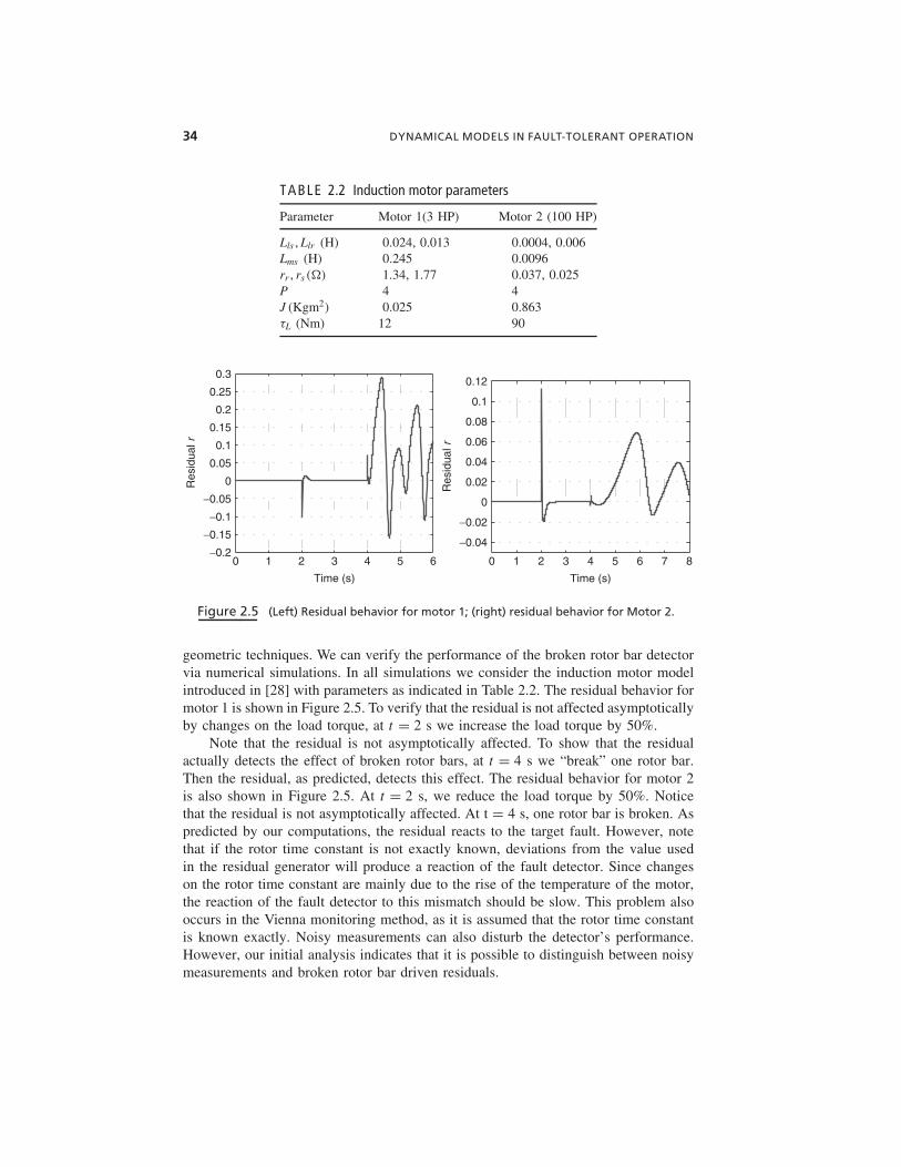
Figure 2.5 (Left) Residual behavior for motor 1; (right) residual behavior for Motor 2.
geometric techniques. We can verify the performance of the broken rotor bar detectorvia numerical simulations. In all simulations we consider the induction motor modelintroduced in [28] with parameters as indicated in Table 2.2. The residual behavior formotor 1 is shown in Figure 2.5. To verify that the residual is not affected asymptoticallyby changes on the load torque, at t = 2 s we increase the load torque by 50%.
Note that the residual is not asymptotically affected. To show that the residualactually detects the effect of broken rotor bars, at t = 4 s we “break” one rotor bar.Then the residual, as predicted, detects this effect. The residual behavior for motor 2is also shown in Figure 2.5. At t = 2 s, we reduce the load torque by 50%. Noticethat the residual is not asymptotically affected. At t = 4 s, one rotor bar is broken. Aspredicted by our computations, the residual reacts to the target fault. However, notethat if the rotor time constant is not exactly known, deviations from the value usedin the residual generator will produce a reaction of the fault detector. Since changeson the rotor time constant are mainly due to the rise of the temperature of the motor,the reaction of the fault detector to this mismatch should be slow. This problem alsooccurs in the Vienna monitoring method, as it is assumed that the rotor time constantis known exactly. Noisy measurements can also disturb the detector’s performance.However, our initial analysis indicates that it is possible to distinguish between noisymeasurements and broken rotor bar driven residuals.
FAULT DETECTION ON POWER SYSTEMS 35
Clearly, the limitations of the developed induction motor model will affect thefault detector scheme. But because we consider ideally distributed stator and rotorwindings, it is not possible to determine the influence of other current harmonics onthe residual.
2.5 FAULT DETECTION ON POWER SYSTEMS
In the new highly interconnected electricity markets, state estimation is the key func-tion in determining real-time network operating conditions. Operators justify technicaland economical decisions based on the network operation conditions, such as manag-ing congestion and uncovering potential operation problems. As a consequence moreaccurate and reliable state estimators are needed.
In power systems practice, state estimation is currently performed in a non–model-based framework. So state estimation is mainly used to filter redundant data,to eliminate incorrect measurements, and to allow for the determination of the powerflows in parts of the network that are not directly metered. There are some state esti-mation procedures that include a simplified dynamics (a first-order dynamic equationdriven by noise) to add pseudomeasurements that help in filtering bad analog data thatmay arise during parameter estimation; observability conditions improve in situationswhere the meter configuration may change during the process. Recently some dynamicmodel-based state estimation approaches have been introduced. For instance, in [5]a gain-scheduled nonlinear observer is introduced to estimate the machine angle in asingle machine infinite bus configuration. In [25] the multimachine state estimationproblem is addressed and solved with a linear observer.
In this section we propose a model-based fault detection scheme for embeddedpower systems. Traditionally fault detection problems in power systems have beenaddressed in a model-free framework. A carefully selected signal is monitored in timeor frequency domain in order to track deviations from its expected value. More elabo-rated monitoring schemes include the identification of false alarms. Since false alarmscould cause costly shutdowns, this state of affairs is not completely satisfactory. Sincethe state estimation is the cornerstone for model-based fault detection, the proposedmonitoring scheme relies in a model-based state estimation process. Two main stum-bling blocks remain on this approach: one is the need to tailor the level of detail forcomponent models (as to keep the overall model tractable) and the other is the needto discriminate the sources of possible misfirings in a systematic fashion. We considerthe dynamics of a power system associated to the swing model, assuming that lineparameters, generator parameters, bus voltage magnitudes, and generator speed areknown. A nonlinear observer is used to estimate a quantity related to the generatorangles, which in turn is used to generate a residual signal. To illustrate the idea, weconsider a very simplified version of the power system of the electric ship presentedin [21].
2.5.1 The Model
We consider the structure-preserving internal-node classical swing model [23]. In thismodel the generator is described by the swing equations, and its effect on the network
36 DYNAMICAL MODELS IN FAULT-TOLERANT OPERATION
is considered as a constant voltage source behind a transient reactance, so that thepower system is described by the differential equations
dδi
dt= ωi − ωs
2Hi
ωs
dωi
dt= TMi − Re(Eqi I
∗Gi ) − Di (ωi − ωs) (2.45)
Eqi ejδi = jX ′
di IGi + Vi ejθi , i = 1, . . . , m
and the load-flow equations
Vi ejθi I ∗
Gi + PLi + jQLi =n∑
k=1
Vi Vk Yik ej (θi −θk −αik ), i = 1, . . . , m
PLi + jQLi =n∑
k=1
Vi Vk Yik ej (θi −θk −αik ), i = m + 1, . . . , n
(2.46)
where δi i = 1, . . . , m are the generator angles, ωi i = 1, . . . , m are the generatorspeeds, ωs is the synchronous speed in p.u., Hi is the inertia in p.u. of generatori , Di is the damping constant in p.u. of generator i , X ′
di is the transient impedance ofgenerator i , TMi is the mechanical torque applied to the generator shaft, Eqi ejδi is theinternal voltage of generator i , IGi is the internal current of generator i , Vi ejθi is thevoltage at bus i , PLi is the active power load at bus i , QLi is the reactive power loadat bus i , and Yik e−jαik is the i , k element of the admittance bus matrix.
Assuming constant load impedances, we can write the differential algebraicequations (2.45)-(2.46) as
dδi
dt= ωi − ωs
2Hi
ωs
dωi
dt= TMi − Re(Eqi I
∗Gi ) − Di (ωi − ωs) (2.47)
[IG
0
]=
[YG YB
Y TB YC
] [EV
]
where
IG = [IG1 . . . IGm
]E = [
Eq1ejδ1 . . . Eqm ejδm]
V = [V1ejθ1 . . . Vm ejθm
]YG = diag
{1
jX ′d1
. . .1
jX ′dm
}
FAULT DETECTION ON POWER SYSTEMS 37
YB = [−YG 0]
YC = Ybus +[
YG 00 0
]+ diag{yL1 . . . yLn}
with Ybus the network admittance matrix and
yLi = PLi − jQLi
V 2i
, i = 1, . . . , n
2.5.2 Class of Events
Here we model three classes of events: bus load changes, symmetrical line shortcircuits, and lost lines.
1. Bus load change. A load change at bus i is modeled adding to the nominaladmittance matrix YC a matrix with all entries equal to zero but the entry(i , i ):
YFlc =i
⎡⎢⎢⎣
0 0 0 00 �ybi 0 00 0 0 00 0 0 0
⎤⎥⎥⎦
i
(2.48)
where
�ybi = �PLi − j�QLi
V 2i
with �PLi and �QLi as the active and reactive power changes, respectively.
2. Symmetrical line short circuit. A symmetrical line short circuit is modeled byadding a virtual bus at the point of the short circuit and by connecting to thevirtual bus a load with very high admittance. For instance, if the short circuitoccurs between buses s and t at 1
βthe length of the line from bus s , the
following admittance matrix is added to YC :
YFsc =
s
t
n + 1
⎡⎢⎢⎢⎢⎢⎢⎣
0 0 0 0 0 00 −αyli 0 yli 0 −αyli
0 0 0 0 0 00 yli 0 −(1 − α)yli 0 −(1 − α)yli
0 0 0 0 0 00 −αyli 0 −(1 − α)yli 0 yli + y0
⎤⎥⎥⎥⎥⎥⎥⎦
s t n + 1
(2.49)
where α = 1/β and y0 represents the added high admittance.
3. Lost line. The effect of losing a line is modeled by removing the line’s admit-tance from the admittance bus matrix. For instance, if the line from bus s
38 DYNAMICAL MODELS IN FAULT-TOLERANT OPERATION
to bus t , with admittance yli , is lost, the following matrix is added to theadmittance bus matrix YC :
Since the events have been modeled as admittance changes, their effects on thepower system dynamics enter through the admittance matrices YB and YC . In thischapter we consider only two events: a load bus change and a lost line. Thus thefaulted admittance matrix YC is defined as
YC = YC + aYFlc + bYFll (2.51)
where a and b take the value 1 when the event is present and the value 0 when it isnot.
2.5.3 The Navy Electric Ship Example
Consider the simplified version, shown in Figure 2.6, of the ship power system intro-duced in [21]. The bus admittance matrix Ybus is defined as
Ybus =⎡⎣ 2ya 0 −2ya
0 2yb −2yb
−2ya −2yb 2(ya + yb
⎤⎦ (2.52)
On the other hand, we have
YG =
⎡⎢⎢⎣
1
jX ′d1
0
01
jX ′d2
⎤⎥⎥⎦ , YB =
⎡⎢⎢⎣
1
jX ′d1
0 0
01
jX ′d2
0
⎤⎥⎥⎦
YC =
⎡⎢⎢⎢⎢⎣
X ′d1(2ya + yM 1) − j
X ′d1
0 −2ya
0X ′
d2(2yb + yM 2) − j
X ′d2
−2yb
−2ya −2yb 2yab + yL3
⎤⎥⎥⎥⎥⎦ (2.53)
where yab = ya + yb . From the last two equations of (2.47) we have
IG = ZE , Z = YG − YB Y −1C Y T
B (2.54)
FAULT DETECTION ON POWER SYSTEMS 39
j Xd
j Xd
y M1
V 1E 1
E 2 V 2
V 3
y L3
y M 2
ya
ya
yb
yb
+−
+−
Figure 2.6 Power system diagram of the Navy electric ship.
Then equation (2.47) for the power system of Figure 2.6 reads as follows:
dδ1
dt= ω1 − ωs
2H1
ωs
dω1
dt= TM 1 − Z r
11E 2q1 − Eq1Eq2Z r
12 cos(δ1 − δ2)
− Eq1Eq2Z i12 sin(δ1 − δ2) − D1(ω1 − ωs)
dδ2
dt= ω2 − ωs (2.55)
2H2
ωs
dω2
dt= TM 2 − Z r
22E 2q2 − Eq1Eq2Z r
21 cos(δ1 − δ2)
+ Eq1Eq2Z i21 sin(δ1 − δ2) − D2(ω2 − ωs)
where Z rij = Re(Zij ) and Z r
ij = Im(Zij ) with Zij the (i , j ) element of Z .Next we consider a load change at bus 1 followed by a loss of the line between
bus 1 and bus 3. These two events are modeled by the following matrices:
YFlc =⎡⎣�yb1 0 0
0 0 00 0 0
⎤⎦ , YFll =
⎡⎣−ya 0 ya
0 0 0ya 0 −ya
⎤⎦ (2.56)
2.5.4 Fault Detection Scheme
Assuming that the events occur independently, we propose the following residualcandidate:
r = (Y TB E + YC V )e−jδ2 (2.57)
40 DYNAMICAL MODELS IN FAULT-TOLERANT OPERATION
the term in parenthesis, under fault free conditions, is equal to zero. Expanding (2.57),we have
The unknown quantities in (2.58) are δ1 − δ2 and V e−jδ2 . In order to compute V e−jδ2 ,we consider the relation
0 = Y TB Ee−jδ2 + YC V e−jδ2 (2.59)
which givesV e−jδ2 = −Y −1
C Y TB Ee−jδ2
Substituting the above into (2.57), we have
r = Y TB Ee−jδ2 + YC (−Y −1
C Y TB Ee−jδ2) (2.60)
that is r = 0. However, in the faulty case, the admittance matrix YC is replaced byYC defined in (2.51), so (2.60) becomes
r = Y TB Ee−jδ2 + (YC + aYFlc + bYFll )(−Y −1
C Y TB Ee−jδ2)
As a consequence the residual candidate r moves away from zero, satisfying the basicrequirements to be considered a true residual. Now, in order to distinguish betweenthe two events, we redefine the residual signal as follows:
rs1 = v1r ,rs2 = v2r
with
v1YFlc �= 0, v1YFll = 0v2YFll �= 0, v2YFlc = 0
(2.61)
so that rs2 �= 0 implies that a line between bus 1 and bus 3 is lost and rs1 �= 0 impliesthat the load at bus 1 has changed. Note that for our example the vectors
v1 = [1 0 1], v2 = [0 0 1]
satisfy (2.61). Then for rs1, mt = a and mn = b while for rs2 we have mt = b andmn = a .
FAULT DETECTION ON POWER SYSTEMS 41
In order to compute the angle δ1 − δ2, we design an observer. To begin, wedefine
δ12 = δ1 − δ2
ω12 = ω1 − ω2(2.62)
Straightforward computations show that in the coordinates (2.62), the power systemdynamic equations (2.55) can be rewritten as
dδ12
dt= ω12 (2.63)
dω12
dt= a1 + a2 cos(δ12) + a3 sin(δ12)
where
a1 = ωs
2H1[TM 1 − Z r
11E 2q1] − ωs
2H2[TM 2 − Z r
22E 2q2]
a2 = ωs
2Eq1Eq2
(Z r
21
H2− Z r
12
H1
)(2.64)
a3 = −ωs
2Eq1Eq2
(Z i
12
H1+ Z i
21
H2
)
and we have disregarded the damping terms.We propose an observer with the following structure:
By linearization it can be shown that for �1 < 1 and �2 > 0 the observation errorseδ = δ12 − δ12 and eω = ω12 − ω12 go asymptotically to zero.
2.5.5 Numerical Simulations
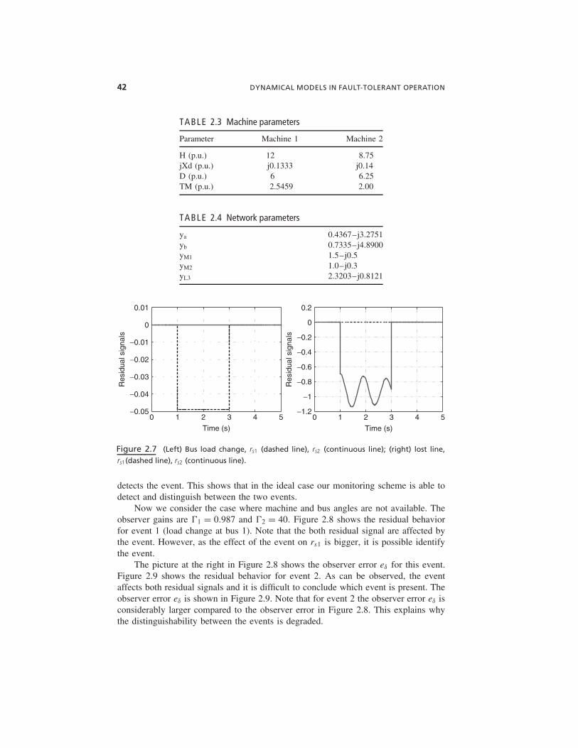
To verify the performance of the monitoring scheme, we carried out numerical simula-tions. The power system parameters are given in Tables 2.3 and 2.4. In all simulationsit is assumed that events do not occur simultaneously and that the power system isinitially at a given equilibrium point. The events occur during 1 ≤ t ≤ 3 s.
First, we consider the ideal case; that is, we assume that machine and bus anglesare available. Figure 2.7 shows the residual behavior for a load change of 0.5 p.u. atbus 1. As expected, the residual signal rs1 moves away from zero while rs2 remainsequal to zero.
The picture at the right in Figure 2.7 shows the residual behavior in the eventof losing a line between bus 1 and 3. Note that as expected, the residual signal rs2
ya 0.4367–j3.2751yb 0.7335–j4.8900yM1 1.5–j0.5yM2 1.0–j0.3yL3 2.3203–j0.8121
Time (s)
0 1 2 3 4 5
Res
idua
l sig
nals −0.2
−0.4
−0.6
−0.8
−1
−1.2
0.2
0
Time (s)
Res
idua
l sig
nals
0
0.01
0
−0.01
−0.02
−0.03
−0.04
−0.051 2 3 4 5
Figure 2.7 (Left) Bus load change, rs1 (dashed line), rs2 (continuous line); (right) lost line,
rs1(dashed line), rs2 (continuous line).
detects the event. This shows that in the ideal case our monitoring scheme is able todetect and distinguish between the two events.
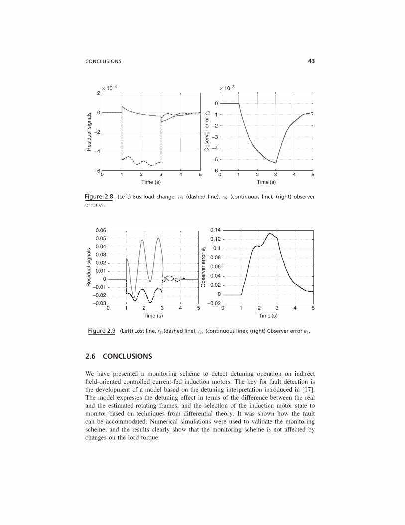
Now we consider the case where machine and bus angles are not available. Theobserver gains are �1 = 0.987 and �2 = 40. Figure 2.8 shows the residual behaviorfor event 1 (load change at bus 1). Note that the both residual signal are affected bythe event. However, as the effect of the event on rs1 is bigger, it is possible identifythe event.
The picture at the right in Figure 2.8 shows the observer error eδ for this event.Figure 2.9 shows the residual behavior for event 2. As can be observed, the eventaffects both residual signals and it is difficult to conclude which event is present. Theobserver error eδ is shown in Figure 2.9. Note that for event 2 the observer error eδ isconsiderably larger compared to the observer error in Figure 2.8. This explains whythe distinguishability between the events is degraded.
We have presented a monitoring scheme to detect detuning operation on indirectfield-oriented controlled current-fed induction motors. The key for fault detection isthe development of a model based on the detuning interpretation introduced in [17].The model expresses the detuning effect in terms of the difference between the realand the estimated rotating frames, and the selection of the induction motor state tomonitor based on techniques from differential theory. It was shown how the faultcan be accommodated. Numerical simulations were used to validate the monitoringscheme, and the results clearly show that the monitoring scheme is not affected bychanges on the load torque.
44 DYNAMICAL MODELS IN FAULT-TOLERANT OPERATION
We also developed a simplified model for a squirrel cage induction motor thatincludes broken rotor bars effects. Relying on differential geometry techniques, wehave proposed a model-based solution to the broken rotor bar detection problem onIFOC-driven squirrel cage induction motors. We show that load torque conditions willnot lead to errors in the detection, as the fault detector is not affected by the loadtorque. Numerical simulations of very different induction motors validate the modeland the performance of the monitoring scheme.
Finally, we addressed the fault detection problem in an embedded power systemand proposed a model-based solution. The distinguishability is achieved in the idealcase. However, as shown by our numerical simulation the capability to distinguishbetween the two events is degraded by the observer performance, ongoing efforts aredirected toward the design of an adaptive observer.
BIBLIOGRAPHY
1. Basille, G., and Marro, G. Controlled and Conditioned Invariants in Linear Systems Theory .Prentice Hall, 1992, ISBN 0-13-172974-8.
2. Beard, R. V. Failure Accommodation in Linear Systems through Self-Reorganization . PhDdissertation. MIT, Cambridge, February 1971.
3. Benbouzid, M. H., and Kliman, G. B. “What Stator Current Processing-Based Technique toUse for Induction Motor Rotor Fault Diagnosis?” IEEE Trans. Energy Conversion , 18(2):238–244, 2003.
4. Burnett, R., Watson, J. F., and Elder S. “The Detection and Location of Rotor Faults withinThree Phase Induction Motors.” Proc. Int. Conf. Electric Machinery , pp. 288–293, 1994.
5. Chang, J., Taranto, G., and Chow, J. “Dynamic State Estimation in Power System UsingHigh Gain-Scheduled Nonlinear Observer.” Proc. 4th IEEE Conf. on Control Applications ,pp. 221–226, 1995.
6. De Persis, C., and Isidori A. “A Geometric Approach to Nonlinear Fault Detection andIsolation.” IEEE Trans. on Automatic Control , 46(6): 853–865, 2001.
7. Filippetti, F., Franchescini, G., and Tassoni, C. “Neural Network Aided On-line Diagnosisof Induction Motor Rotor Faults.” IEEE Trans. Industrial Applications , 31(4): 892–899,1995.
8. Gertler, J., All Linear Methods are Equal and Extendible to (Some) Nonlinearities.’’ Int.J. Robust Nonlinear Control , 12: 629–648, 2002.
9. Hammouri, H., Kinnaert, M., and El Yaagoubi, E. H. “Fault Detection and Isolation forState Affine Systems.” European Journal of Control , 4(11): 2–16, 1998.
10. Jones, H. L. Failure Detection in Linear Systems . PhD dissertation. MIT, 1973.
11. Karagiannis, D., Astolfi, A., and Ortega, R. “Two Results for Adaptive Output FeedbackStabilization of Nonlinear Systems.” Automatica, 39(5): 857–866, 2003.
12. Kral, C., Pirker, F., and Pascoli, G. “Detection of Rotor Faults in Squirrel-Cage InductionMachines at Standstill for Batch Test by Means of the Vienna Monitoring Method.” IEEETrans. Industry Applications , 38(3): 618–624, 2002.
13. Krause, C. P., Wasynczuk, O. and Sudho, D. S. Analysis of Electric Machinery . IEEE Press,New York, 1995.
BIBLIOGRAPHY 45
14. Manolas, S. T. J., and Tegopoulos, J. A., “Analysis of Squirrel Cage Induction Motors withBroken Bars and Rings.” IEEE Trans. Energy Conversion , 14(4): 1300–1305, 1999.
15. Massoumnia, M. “A Geometric Approach to the Synthesis of Failure Detection Filters.”IEEE Trans. Automatic Control , 31(9): 839–846, 1986.
16. Massoumnia, M., Verghese, G., and Willsky, A. “Failure Detection and Identification.”IEEE Trans. Automatic Control , 34(3): 316–321, 1989.
17. Mijalkovic, M. Sensitivity Analysis for Nonlinear Magnetics . Northeastern University Inter-nal Report, May, 2002.
18. Mohan, N. Advanced Electric Drives . MNPERE, Minneapolis, MN, 2001.
19. Novotny, D. W., and Lipo, T. A. Vector Control and Dynamics of AC Drives . ClarendonPress, New York, 1996.
20. Patton, R., Frank, P., and Clark R. Fault Diagnosis in Dynamic Systems Theory and Appli-cation . Prentice Hall, Upper Saddle River, NJ, 1989.
21. Pekarek, S., Tichenor, J., Benavides, N., Koeing, A., Wang, H., Sudho, S., Kuhn, B.,Glover, S., Aliprantis, D., Byoun, J., and Sauer, J. Development of a Test Bed for Designand Evaluation of Power Electronic Based Systems . Society of Automotive Engineers, Troy,MI, 2002.
22. Ritchie, E., Deng, X., and Jokinen, T. “Diagnosis of Rotor Faults in Squirrel Cage InductionMotors Using a Fuzzy Logic Approach.” Proc. Int. Conf. Electric Machinery , Paris, France,pp. 348–352, 1994.
23. Sauer, P. W., and Pai, M. A. Power System Dynamics and Stability . Prentice Hall, UpperSaddle River, NJ, 1998.
24. Schoen, R. R., and Hableter, G. T. “Evaluation and Implementation of a System to EliminateArbitrary Load Effects in Current–Based Monitoring of Induction Machines.” IEEE Trans.Industry Applications , 33(6):, 1997.
25. Scholtz, E., Sonthikorn, P., Verghese, G. C., and Leisure, B. C. “Observers for Swing StateEstimation of Power Systems.” Proc. North American Power Symp., October, 2002.
26. Thomson, W. T., and Fenger, M. “Current Signature Analysis to Detect Induction MotorFaults.” IEEE Industry Applications , July–August: 26–34, 2001.
27. Watson, J. F., and Elder, S. “Transient Analysis of the Line Current as a Fault Detec-tion Technique for 3-phase Induction Motors.” Proc. Int. Conf. Electric Machinery , pp.1241–1245, 1992.
28. Welsh, M. S. Detection of Broken Rotor Bars in Induction Motors Using Stator Measure-ments . PhD dissertation. MIT, Cambridge, May 1988.
29. Williamson, S., and Smith A. C. “Steady-State Analysis of 3-phase Cage Motors with RotorBar and End Ring Faults.” Proc. Institute of Electrical Engineering , 2(3B): 93–100, 1982.