Operational algorithm for ice–water classification ondual-polarized RADARSAT-2 imagesNatalia Zakhvatkina1,2, Anton Korosov3, Stefan Muckenhuber3, Stein Sandven3, and Mohamed Babiker3
1Nansen International Environmental and Remote Sensing Centre (Nansen Centre, NIERSC), 14th Line 7,Office 49, Vasilievsky Island, St. Petersburg, 199034, Russian Federation2Arctic and Antarctic Research Institute (AARI), Bering Str. 38, St. Petersburg, 199397, Russian Federation3Nansen Environmental and Remote Sensing Center (NERSC), Thormøhlensgate 47, 5006 Bergen, Norway
Received: 30 May 2016 – Published in The Cryosphere Discuss.: 21 June 2016Revised: 23 October 2016 – Accepted: 6 December 2016 – Published: 11 January 2017
Abstract. Synthetic Aperture Radar (SAR) data fromRADARSAT-2 (RS2) in dual-polarization mode provide ad-ditional information for discriminating sea ice and open wa-ter compared to single-polarization data. We have developedan automatic algorithm based on dual-polarized RS2 SARimages to distinguish open water (rough and calm) and seaice. Several technical issues inherent in RS2 data were solvedin the pre-processing stage, including thermal noise reduc-tion in HV polarization and correction of angular backscatterdependency in HH polarization. Texture features were ex-plored and used in addition to supervised image classificationbased on the support vector machines (SVM) approach. Thestudy was conducted in the ice-covered area between Green-land and Franz Josef Land. The algorithm has been trainedusing 24 RS2 scenes acquired in winter months in 2011 and2012, and the results were validated against manually derivedice charts of the Norwegian Meteorological Institute. The al-gorithm was applied on a total of 2705 RS2 scenes obtainedfrom 2013 to 2015, and the validation results showed that theaverage classification accuracy was 91± 4 %.
1 Introduction
Synthetic Aperture Radar (SAR) is an active microwave sen-sor providing high-resolution images over large areas inde-pendent of clouds and daylight. This is especially useful forobserving the polar regions, where SAR data are widely usedfor exploring sea ice concentration, extent, detection of leads,polynyas, ice floes and ice edge, and ice type identification
and classification (Johannessen et al., 2007; Dierking, 2013).Monitoring of sea ice processes, i.e., ice edge variations andmotion, is important for practical tasks such as ice navigationand for scientific studies. High-resolution data from C-bandSAR such as ERS-1/2 (European Remote Sensing satellites,European Space Agency, ESA), RADARSAT-1 (Earth ob-servation satellite, Canadian Space Agency), and ENVISAT(Environmental Satellite, ESA) have been used as the maindata source for sea ice monitoring in the last 2 decades (e.g.,Johannessen et al., 2007). The advanced capabilities of SARon board of RADARSAT-2 (RS2) and Sentinel-1 (EuropeanCommission and ESA) with multi-polarization data can im-prove sea ice observations such as ice edge detection and icetype classification.
SAR images can be used to identify different sea icetypes and open water (OW) areas based on variations of thebackscattered radar intensity caused by surface roughnessand other sea ice properties. Classification methods basedonly on the backscattering coefficients (σ ◦) are hampered byambiguities in the relation between ice types and σ ◦, sincevarious ice types (multiyear, first-year, and some young andnew ice) and open water depending on wind speed and direc-tion can have similar σ ◦ (Dierking, 2010; Johannessen et al.,2007). In particular, discrimination between calm open wa-ter and smooth first-year ice, as well as between windy openwater and young ice with frost flowers or multiyear ice, canbe problematic. Including additional image characteristicslike image texture, tone, and spatial structures can improvethe classification results significantly (Shokr, 1991; Soh and
Published by Copernicus Publications on behalf of the European Geosciences Union.
34 N. Zakhvatkina et al.: Operational algorithm for ice–water classification
Tsatsoulis, 1999; Clausi, 2002; Bogdanov et al., 2005; Mail-lard et al., 2005; Yu et al., 2012).
Numerous efforts have been made to develop algorithms toretrieve sea ice variables from SAR data. The SAR polynyadetection algorithm proposed by Dokken et al. (2002) isbased on wavelet transforms for edge detection and standardtexture analysis. A threshold function using texture informa-tion is used to classify sea ice and water for polynya detec-tion. A semi-automated sea ice classification method basedon fuzzy rules was reported by Gill (2003) for classificationof RADARSAT-1 data over the Arctic into calm water, wind-roughened water, and sea ice in low and high concentrations.Advanced Reasoning using Knowledge for Typing of Sea Ice(ARKTOS) (Soh et al., 2004) has been established to sup-port scientific research and operational applications in thefield of sea ice segmentation and classification. Haarpainterand Solbø (2007) developed an automatic algorithm for ice–ocean discrimination in RADARSAT-1 and ENVISAT SARimagery. The texture-based algorithm consists of an automat-ically trained maximum likelihood classifier and divides theSAR images into slices of small incidence angle ranges. Theresults show that sea ice and water can be discriminated quitereliably. Some examples showed a tendency of the algorithmto a better performance at low incidence angles. Karvonen etal. (2005) distinguished the Baltic Sea ice from open waterbased on thresholding of segment-wise local autocorrelationsin SAR images. The method provided 90 % accuracy com-pared to digital ice charts for the Baltic Sea. This algorithmhas been used by the Finnish Meteorological Institute (FMI).Tests with RADARSAT-2 and ENVISAT SAR data show thatover 89.4 % of the test data fit the ice classification providedby the Finnish Ice Service for the Baltic Sea and Arctic Sea(Karvonen, 2010, 2012).
Dual polarization has several advantages for sea ice clas-sification compared to single-polarization SAR data. Roughor frost-flower-covered young ice and multiyear ice, whilevery different in their thickness (10–15 cm and more than2.5 m, respectively), show rather similar brightness in theHH channel whereas MYI is brighter than young ice in theHV channel. Smooth first-year level ice is darker in bothHH and HV and can be easily distinguished from youngice and MYI. Wind-roughened open water is difficult to dis-tinguish from sea ice in a single HH polarization. How-ever, open water especially affected by wind is darker in HVthat improves sea ice classification (Sandven et al., 2008).The dual-polarization ENVISAT SAR Alternative Polariza-tion Mode data enabled discrimination of sea ice types andopen water with a decision-tree classifier using estimatedstatistical thresholds for winter. Open water can be unam-biguously discriminated from smooth FYI, rough FYI, andMYI with > 99 % accuracy using a co-polarized ratio thresh-old (Geldsetzer and Yackel, 2009). The possibilities of su-pervised k-means and maximum likelihood classification ofvarious SAR polarimetric data to three pre-identified sea ice
types and wind-roughened open water was explored in Gilland Yackel (2012).
The MAp-Guided Sea Ice Classification System (MAGIC)for automated ice–water discrimination on dual-polarizationimages from RADARSAT-2 combines a “glocal” IterativeRegion Growing using Semantics (IRGS) classification (Yuand Clausi, 2008) with a pixel-based support vector machine(SVM) approach. The “glocal” classification identifies ho-mogeneous regions with arbitrary class labels. The ice–watermap is created with the SVM classifier exploiting SAR tex-ture and backscatter features. The MAGIC system has beenapplied on 20 RS2 scenes over the Beaufort Sea. The aver-age classification accuracy with respect to manually drawnice charts is 96.5 % (Clausi et al., 2010; Ochilov and Clausi,2012; Leigh et al., 2014).
A neural-network-based algorithm has been developed forENVISAT SAR images for operational sea ice classifica-tion including validation (Zakhvatkina et al., 2013). The al-gorithm discriminated the level FYI, deformed FYI, MYI,and open water/nilas in the high Arctic in winter conditionsand demonstrated good applicability in the central Arctic.Using the same approach an algorithm for mapping ice–water utilizing ENVISAT ASAR WSM images was createdfor automated ice edge detection in Fram Strait. The ice–water classes were estimated by a multi-layer perceptronneural network which uses SAR calculated texture featuresand concentration data from AMSR (Advanced MicrowaveScanning Radiometer) and, later, SSM/I (Special Sensor Mi-crowave/Imager) as inputs (Sandven et al., 2012). Daily ice–water products were provided with a resolution of 525 mfrom winter 2011 until April 2012. The accuracy of this clas-sification was about 97 % compared to high-resolution seaice concentration charts based on manual interpretation ofsatellite data provided by the Norwegian Meteorological In-stitute.
Our goal is to extend the method originally used for thesingle polarized ENVISAT SAR images (Sandven et al.,2012) by utilizing dual-polarization data from RS2 and todevelop an algorithm for ice–water classification, which canbe applied to RS2 data for the production of ice–water mapsas part of marine services under the Copernicus programme.A special motivation for our work was not only developmentof an algorithm but also its extensively validation in varioussea ice conditions and identification of the applicability con-ditions. We also aimed to develop the algorithm as an open-source software available for other scientists. Our algorithmis based on texture features and the SVM method using theadvantages of dual-polarization RS2 SAR image data.
This paper describes the developed algorithm and dis-cusses practical issues of its applicability. The steps and pa-rameters for implementation of the algorithm are described,allowing users to test the algorithms themselves. The paperis organized as follows. Section 2 introduces the satelliteimages and geographical area used in the study. The algo-rithm including pre-processing and validation procedure is
The Cryosphere, 11, 33–46, 2017 www.the-cryosphere.net/11/33/2017/
N. Zakhvatkina et al.: Operational algorithm for ice–water classification 35
described in Sect. 3. Results of the pre-processing step, ice–water classification, and comparison with manual ice chartsare given in Sect. 4. Finally, a discussion of the results is pre-sented in Sect. 5.
2 Data
The region of interest is the ice-covered sea between Green-land and Franz Josef Land, where detailed ice informationfrom SAR data is important due to the highly variable sea iceconditions, in particular the export out of the Arctic throughFram Strait (Vinje and Finnekåsa, 1986). SAR is the mostuseful sensor to provide high-resolution year-round data forestimation of sea ice variables such as ice classification, iceedge variability, and ice drift.
This study is based on RS2 ScanSAR Wide (SCW)mode images with 500 km swath width, a pixel spacing of50× 50 m, and dual-polarization (HH+HV). This is themain mode used by RS2 for operational sea ice monitoring(RS2 Product Description, 2011). Twenty-four SCW scenesaround Svalbard (Fig. 1) from 2011 and 2012 were utilizedin the following analysis to train the algorithm. The winter-month images were selected to cover various types of thin(e.g., new and young ice), first-year, and multiyear ice withdifferent degrees of deformation, packed ice, broken ice, andopen water under different wind speed conditions (rough,very rough, and calm water, also in leads). The radar imagesinclude the most typical samples since the radar intensitycontrast between open water and ice varies greatly with iceconditions and wind speed or direction which significantlyaffect the radar brightness of open water. In summer the con-trast between backscatter intensities of the melted differentice types observed on the SAR image is diminished sincesurfaces become smoother and are covered by meltwater. Theintensities are reduced as well as the contrast between ice andOW.
The backscatter at HH generally decreases with increas-ing incidence angle (Fig. 2a), whereas the HV channel is lesssensitive to the incidence angle. The HV channel includesdisturbances in azimuth direction (visible as bright and darkstripes) along the burst boundaries in the ScanSAR WideBeam SAR image (Fig. 2b). The expected noise level is alocal mean noise power value that fluctuates across the im-age. The noise level is obtained from a model that accountsfor the characteristics of the SAR sensor, the beam mode, theacquisition, and the ground processing (RS2 PUG) (Jefferies,2012). The system noise level as a function of the incidenceangle is documented in the XML file that comes with the RS2image.
3 Methodology
3.1 Incidence angle correction for HH
During the first step of our ice–water classification algorithmSAR data pre-processing is conducted, including incidenceangular correction for HH and absolute calibration to ob-tain σ ◦ values. The auxiliary XML files coming with theproduct, i.e., scaling look-up table (LUT), provide informa-tion for georeferencing and calibration. These LUTs allowconverting the processed digital numbers of the output SARimage to calibrated values. An important goal of radiomet-ric calibration is to provide the proper comparison betweenthe scattering of image targets with different SAR sensors orfrom the same sensor with different operating conditions, sothe backscatter values of targets can be compared to one an-other or a reference. Absolute radiation calibration is used toconvert the digital numbers in the SAR image to σ ◦, apply-ing a constant offset and range dependent gains to the SARimage (RS2 Product Description, 2011). All images are cor-rected to a reference angle of 35◦, which represents the centerincidence angle and allows analysis of the SAR images with-out brightness amplification. Backscatter recalculation to 35◦
incidence angle is carried out using a predefined calculatedcoefficient:
σj◦= 10 · log10
(
digital number2j
)Aj
· sin(θj)
−(coefficient ·
(θj − 35
)), (1)
where σ ◦ is the backscatter values of pixels in jth line (rangedirection), given in dB; digital number is the pixel brightness(data consist of the SAR amplitude value Amp and intensityvalue I=Amp2; A is the gain value (invariant in line) corre-sponding to the range sample j (obtained by linear interpo-lation of the LUT supplied gain values); θ is the incidenceangle for each jth pixel; and coefficient is the predefined cal-culated coefficient.
The coefficient was defined by calculating the linear trendof the observed backscatter signal on several HH-polarizedRS2 SCW images of pack ice. The procedure is similar tothe pre-processing of ENVISAT ASAR data in Zakhvatkinaet al. (2013). The backscatter normalization to a pre-definedincidence angle provides homogenous image contrast acrossthe swath over ice-covered areas. The details of the angularcorrection method are discussed in Sect. 5.1.
3.2 Thermal noise correction for HV
SAR data pre-processing also includes reduction of ther-mal noise effect and absolute calibration for HV. The ther-mal noise reduction consists of three steps: (1) reading thenoise values and corresponding incidence angles from theXML file, (2) interpolation of noise on a finer grid for each
www.the-cryosphere.net/11/33/2017/ The Cryosphere, 11, 33–46, 2017
36 N. Zakhvatkina et al.: Operational algorithm for ice–water classification
Figure 1. Location of RADARSAT-2 image used for training. All data are provided in GeoTIFF format with auxiliary XML files.
Figure 2. RS2 SCW dual-polarization image taken over Fram Strait on 28 November 2011 prior pre-processing. (a) HH channel with angulardependence; (b) HV channel with noise floor variations.
pixel, and (3) subtraction of interpolated noise values fromthe backscatter values of the entire image.
Due to the discontinuity of the noise floor at the bound-aries of the individual SAR beams and the low resolution ofthe provided noise values in the XML file (only 100 pointsfor 500 km swath width), the noise correction may result inan erroneous subtraction of a high noise floor from a low sig-nal of the neighboring SAR beam and, hence, yield negativevalues for σ ◦. To prevent such flaws, a 10 pixel wide stripe
of data along the edge of the SAR beam is masked out anddisabled for further analysis.
3.3 Manual classification
The second step includes manual classification of SAR im-ages into predefined classes (e.g., open water and ice ofvarious types depending on which classes are needed). Thepredefined classes take into account information from opti-cal data, ice concentration from passive microwave, previousclassification results, and historical data.
The Cryosphere, 11, 33–46, 2017 www.the-cryosphere.net/11/33/2017/
N. Zakhvatkina et al.: Operational algorithm for ice–water classification 37
Manual classification has been done for the training im-ages containing several different sea ice types and ice-freeareas with both rough and smooth open water. Predominantsubclasses, which must be reliable and of high quality, wereidentified and chosen by sea ice experts through visual anal-ysis of RS2 scenes based on their previous experience. Theimages selected for our algorithm training did not containhomogeneous ice cover because the mixing of different icetypes with different degrees of deformation, cracks, ridgesand leads usually occurs in ice-covered areas. The main class“sea ice” was chosen to include the following subclasses:(1) subclass including young ice, first-year, and multiyearice; (2) fast ice; and (3) broken ice on the edge (border) mixedwith ice-free areas (mostly found in the marginal ice zone).The class “open water” included the two subclasses open wa-ter with high and very high wind speed conditions and a thirdsubclass that represented a mixture of calm open water, frazilice, leads, and nilas. These manual classification results werecollocated with texture feature images (description providedin Sects. 3.4 and 4.2) to get a number of training vectors. Forthe final product the subclasses were merged into the mainclasses “sea ice” and “open water” since the similarities be-tween the subclasses are too high for a reliable discriminationwithout additional data.
3.4 Calculation of texture features
The third step is a calculation of texture features from HHand HV images. The calculation of texture features con-sists of the computation of the gray level co-occurrence ma-trix (GLCM) using Eq. (2) and the calculation of texturefeatures based on the GLCM (Eqs. 3–10). Considering thefull range of possible brightness levels (e.g., 0–255) and asmall window size, most GLCM elements would be zero andthat would have a negative effect on the classification result.Therefore we divide the full brightness range into few inter-vals (quantization levels K). The GLCM is created for eachdirection θ , where each cell (i, j) is a measure of the rel-ative frequency of two pixels occurrence with brightness iand j, respectively, separated by a co-occurrence distance d.One may also say that the matrix element Pd,θ (i, j) is a mea-sure of the second-order statistical probability for changesbetween gray levels i and j at a particular displacement dis-tance d and at a particular angle (direction) (θ). The size ofsquare GLCM is equal to number of quantized brightnesslevels K. The GLCM is averaged over four directions θ (0,45, 90, 135◦) to account for possible rotation of the ice floes(Clausi, 2002; Haralick et al., 1973).
Sd,θ (i,j)=Pd,θ (i,j)∑K
i=1∑Kj=1Pd,θ (i,j)
, (2)
where Sd,θ is the GLCM, Pd,θ is the number of neighborpixel pairs, θ is the fixed vector directions (0, 45, 90, 135◦),d is the co-occurrence distance, K is the number of quantized
gray levels, and i, j are the gray levels (0–255).
Energy=∑K
i=1
∑K
j=1
[Sd,θ (i,j)
]2 (3)
Homogeneity=∑K
i=1
∑K
j=1
Sd,θ (i,j)
1+ (i− j)2(4)
Contrast=∑K
i=1
∑K
j=1(i− j)2Sd,θ (i,j) (5)
Correlation=
∑Ki=1∑Kj=1 (i−µx)
(j −µy
)Sd,θ (i,j)
σxσy(6)
Entropy=−∑K
i=1
∑K
j=1Sd,θ (i,j) log10Sd,θ (i,j) (7)
Kurtosis=∑K
i=1
∑K
j=1
(Sd,θ −µ
)4σ 4 (8)
Skewness=∑K
i=1
∑K
j=1
(Sd,θ −µ
)3σ 3 (9)
Cluster prominence=∑K
i=1
∑K
j=1
(i+ j −µx −µy
)4Sd,θ (i,j) (10)
σ 2x =
K∑i=1
K∑j=1
(j −µx)2Sd,θ (i,j) and σ 2
y =
K∑i=1
K∑j=1
(j −µy
)2Sd,θ (i,j) are standard devia-
tion of rows and columns, µx =K∑i=1
K∑j=1
iSd,θ and
µy =K∑i=1
K∑j=1
jSd,θ are mean values of rows and columns,
σ 2=
K∑i=1(i−µ)2
K∑j=1
Sd,θ (i,j) is the standard deviation,
and µ=K∑i=1
K∑j=1
iSd,θ (i,j) is the mean values of brightness.
The results of this procedure depend on several factorssuch as the size of the sliding window, the co-occurrencedistance, and the quantization levels (Shokr, 1991; Soh andTsatsoulis, 1999; Clausi, 2002). In order to test the effects ofthese parameters on the classification accuracy, texture fea-tures were calculated for the window sizes 16, 32, 64, and128 pixels using different co-occurrence distances and vary-ing the number of quantized gray levels (Table 1). The opti-mal values for the parameters of texture features calculationwere selected analyzing variations in the texture parametersby visual inspection of the normalized mean values distribu-tion of each texture feature for a defined class. The decisionis made for the benefit of the cases when the separation of thenormalized texture values for the classes increases in the ma-jority of investigated texture feature figures. Defined parame-ters were applied for calculations of all set of texture features,and then the visual comparison showed the best discrimina-tion between the ice–water classes for some texture features(details provided in Sect. 4.2).
www.the-cryosphere.net/11/33/2017/ The Cryosphere, 11, 33–46, 2017
38 N. Zakhvatkina et al.: Operational algorithm for ice–water classification
Table 1. Experiments of computation parameters. W is the windowsize, d is the co-occurrence distance, K is the quantized gray level,and moving step is a step of sliding window moving.
A selection procedure is applied to limit a set of tex-ture characteristics that provides a good classification witha small computational load. This procedure includes visualassessment of scatter plots, comparing values of texture fea-tures in different combinations. Candidate texture featuresthat provide the best separation of classes are selected andothers are discarded. The selection procedure also uses a setof training images to establish the set of texture features andits computation parameters, providing the smallest classifi-cation error. In other words, we constrain the texture featuresnumber by the demanded balance considering the SAR im-age level of details, computation time, and the optimal reli-able class separation.
3.5 Support vector machines
The next step is the training of classifier (e.g., SVM) forclassification of arrays with certain texture features as wellas σ ◦ values based on the results of manual classification.The SVM are supervised learning methods with associatedlearning algorithms that provide data classification. The ba-sic SVM takes a set of input data (several “attributes”, i.e.,the features) and predicts the outputs (i.e., the class labels)for each given input, making it a non-probabilistic classifier.The support vector network maps the input vectors into ahigh dimensional feature space through nonlinear mapping.SVM finds a linear hyperplane separating objects into classesby the most widely clear gap between the nearest trainingdata points of any class. An optimal hyperplane is definedas the linear decision function with maximal margin betweenthe vectors in this higher dimensional space. When the maxi-mum margin is found, only points which lie closest to the hy-perplane have weights > 0. These points determine this mar-gin and are called support vectors (Cortes and Vapnik, 1995).
SVM performs a nonlinear classification using the ker-nel trick. The kernel function may transform the data into
a higher dimensional space to make this nonlinearly separa-tion possible when the relation between class labels and at-tributes is nonlinear. A common choice is a Gaussian kernel.In our study we have used the radial basis function kernel(RBF kernel), which is found to work well in a wide varietyof applications.
The scikit-learn open source was used to implementthe SVM classification method (http://scikit-learn.org/stable/index.html). SVM models implementation in scikit-learn isbased on LIBSVM. Basically, SVM trains the model usinglow-level method and can only solve binary classificationproblems. In the case of multi-class classification, LIBSVMimplements the “one-against-one” technique by fitting all bi-nary sub-classifiers and finding the correct class by a vot-ing mechanism. The effectiveness of SVM training dependson the selection of kernel, the kernel’s parameters (γ ), andmargin parameter C. The software provides a simple tool tocheck a grid of parameters obtaining cross-validation accu-racy for each parameter setting: the parameters with the high-est cross-validation accuracy are returned (Hsu et al., 2003).The SVM parameters in our case were γ = 0.1 and C = 1.
The calculated texture features and σ ◦ values corre-sponding to the manually identified classes on several pre-processed RS2 images were used as input data for trainingthe SVM classifier. After completing the training procedurethe resulting SVM is applied for automatic sea ice classifica-tion to divide the RS2 scene into the predefined classes.
3.6 Validation
The final step includes validation of the classification re-sults using manually drawn ice charts. Validation of Arcticsea ice classification results is a challenging task since seaice is a very inhomogeneous medium and validation dataon ice classification are difficult to obtain. As a substituteour sea ice classification results have been compared withmanual sea ice charts produced by the operational ice ser-vice at the Norwegian Meteorological Institute (MET Nor-way, http://polarview.met.no/). MET Norway produces icecharts every workday using the following data sources: high-resolution SAR images, low-resolution microwave SSM/Iand SSMIS data (DMSP), MODIS images (Terra and Aqua),and AVHRR data from NOAA. In our comparison MET Nor-way ice charts are assumed to represent “true” classificationand the confusion matrix was calculated for accuracy evalu-ation of our algorithm results.
After completing the algorithm training, the fully auto-mated image classification includes only three of the abovementioned steps: pre-processing (Sect. 3.1 and 3.2), texturefeature retrieval (Sect. 3.4), and application of the automaticclassifier (SVM).
The initial size of the full-resolution RS2 SCW image isabout 10 000× 10 000 pixels. We downscale the original im-age by averaging to 5000× 5000 pixels to increase the com-putational efficiency and decrease the influence of speckle
The Cryosphere, 11, 33–46, 2017 www.the-cryosphere.net/11/33/2017/
N. Zakhvatkina et al.: Operational algorithm for ice–water classification 39
noise. The image size is further reduced during the com-putation of the texture features by using a sliding windowwith 16 pixel step size (the detailed parameters are describedin Sect. 4.2). The image size of the final product is about330× 330 pixels with 1600 m pixel spacing. This reductionin resolution significantly increases the processing speed andallows computing a classification results in less than 15 min.
Pre-processing of RS2 data was performed utilizing theopen-source Python toolbox NANSAT (Korosov et al.,2015), (https://github.com/nansencenter/nansat/wiki). Thetexture extraction algorithm was created in the Python pro-gramming language.
4 Results
To illustrate the algorithm performance the automatic SVMclassification was applied to the RS2 scene shown in Fig. 2.The example scene was acquired on 28 November 2011 overthe western part of Svalbard in Fram Strait. Figures 2 and 3show both HH and HV polarizations before and after corre-sponding corrections described in Sect. 2: compensation ofincidence angle effects for HH (Fig. 3a) and noise reductionfor HV (Fig. 3b). The image contains several ice types, openwater under different wind conditions, and land. The openwater area is located on the right-hand side of the image andthe ice-covered area in the upper-left corner. The sea ice areaincludes a marginal ice zone with bright broken up ice. Theice-covered areas and the rough OW areas appear both brightin HH and are therefore difficult to distinguish. Including HV,however, provides additional information since OW areas onthis image appear generally darker than sea ice in HV. Thisis one of the major dual-polarization advantages and can beseen in the lower right part of the example image (Fig. 2).
4.1 Correction for incidence angle and thermal noise
The linear trend coefficient used for backscatter angu-lar dependence correction of HH was estimated to be−0.298 dB/1◦ and allowed normalization of σ ◦ to the inci-dence angle 35◦ as shown on Fig. 3a and c. The application ofour noise correction procedure for HV reduces significantlythermal noise and gets rid of vertical striping as shown inFig. 3b, d.
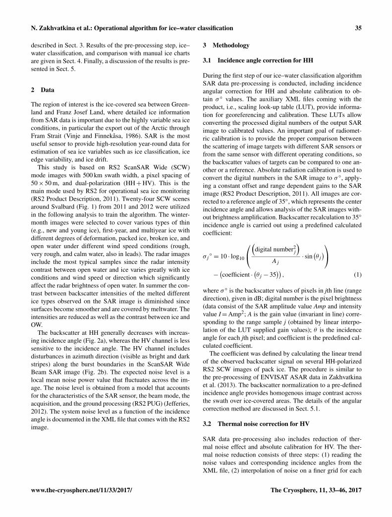
4.2 Texture feature calculation
As part of the algorithm development texture features werecalculated based on different parameter settings. Visualexamination of mean values of several texture features(Fig. 4a, b) suggested the optimal combination of the slidingwindow, moving step, and distance between neighboring pix-els, which provides better separation of the ice–water classescompared to other combinations of window sizes with dif-ferent texture parameters. A set of texture characteristics wasselected analyzing variations in mean values of the textu-
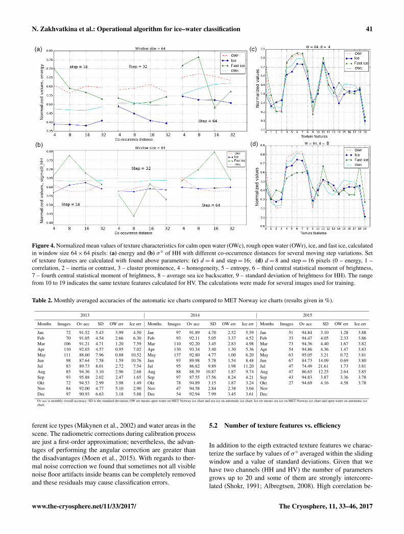
ral characteristics of defined classes calculated with severalcombinations of obtained parameters (Fig. 4c, d). The largestchange of distance between mean values of texture featuresof different classes on Fig. 4d defines the best option forthe potential classification. Finally, together with visual in-spection of the texture images (some examples are given onFig. 5a–f) of the a priori known most problematic classifi-cation cases on the SAR images used for training, the setof texture characteristics are defined. The best results wereachieved using the following parameter set: number of graylevels (K= 32), co-occurrence distance (d= 8), sliding win-dow size (w= 64× 64), and moving step of the sliding win-dow (s= 16). Using the following texture features for thetwo channels provided the best test results: for HH channelthe energy, inertia, cluster prominence, entropy, third statis-tical moment of brightness, backscatter, and standard devia-tion were calculated; for HV channel the energy, correlation,homogeneity, entropy, and backscatter were calculated. In-cluding more texture features for both channels was testedbut found not to improve the information content. The calcu-lation parameters were found experimentally to give a goodcompromise between speckle noise reduction, preservationof details, and correct classification results (methodology de-scription in Zakhvatkina et al., 2013).
Texture characteristics provide a more complete delin-eation of surface parameters in addition to the raw backscat-ter signal, and increase the ability for ice and water separa-tion. The scatter plots in Fig. 5g, h show the values of twodifferent texture features plotted against each other and il-lustrate the usefulness of texture features for discriminationbetween defined classes.
4.3 Manual versus automatic classification
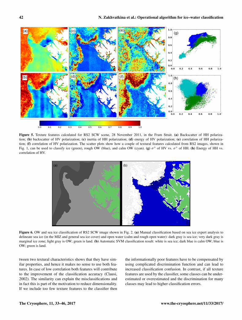
As described in Sect. 3 several SAR images were classifiedmanually as part of the training procedure for the automaticalgorithm. Comparing the manual classification from sea iceexpert analysis with the algorithm results (Fig. 6) reveals ageneral high level of correspondence and illustrates the capa-bility of the automatic approach. Detailed observation of theclassification results show that most misclassifications areobserved near land and in the MIZ. Figure 6b shows smallfeatures inside ice-covered zone (blue dots) that were mis-classified as OW.
4.4 Validation
Validation of the algorithm results has been performed us-ing 2705 RS2 images taken over our area of interest in theperiod 1 January 2013 until 25 October 2015. For each RS2image an error matrix based on pixel-by-pixel difference be-tween algorithm result and MET Norway chart has been cal-culated. OW and sea ice correspondence as well as an over-all accuracy were obtained for each RS2 image classifica-tion result and averaged accuracies have been calculated for
www.the-cryosphere.net/11/33/2017/ The Cryosphere, 11, 33–46, 2017
40 N. Zakhvatkina et al.: Operational algorithm for ice–water classification
Figure 3. RS2 SCW dual-polarization image taken over Fram Strait on 28 November 2011, including pre-processing. (a) Calibrated imageafter correction of σ ◦ at 35◦ incidence angle using the predefined coefficient for sea ice of −0.298 dB/1◦. (b) Noise-corrected image: beamboundaries are visible due to differences in noise levels between adjacent beams. (c) σ ◦ curves of SAR image across the entire swath: originalimage (blue) and after angular correction (green). (d) σ ◦ curves of SAR image along the whole swath. The blue curve shows σ ◦ value profileof the raw HV channel image in range direction, the red curve depicts the noise floor level, and the green curve is the result of subtraction.
each month. The impact of each class on the classificationerror has been estimated and the respective monthly aver-aged errors were computed. The averaged overall accuraciesincluding standard deviation and errors in ice and water clas-sification for each month are given in Table 2. In addition,the monthly accuracies are presented as a graph in Fig. 7.The monthly averaged overall accuracies show lower valuesduring summer months (Fig. 7 – from May to October) andhigher values during winter. The average total classificationaccuracy for all 2705 scenes is 91± 4 %.
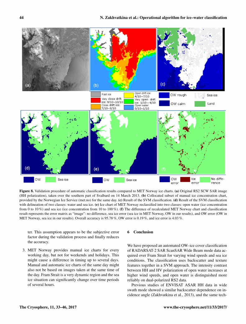
Figure 8 shows an example of the validation process. TheRS2 HH image is shown in Fig. 8a, the result of our SVMclassification in Fig. 8c, and the MET Norway sea ice chartin Fig. 8b. To compare the algorithm result with the manu-ally derived ice charts, both products are reclassified into iceand water (Fig. 8d and e). The error matrix is represented asan image (Fig. 8f) with the following three classes: no differ-ence, sea ice error (MET Norway: sea ice, OW in our results),and OW error (MET Norway: OW, sea ice in our results).
5 Discussion
5.1 Significance of incidence angle variations andthermal noise reduction
Water areas have a very large range of brightness dependingon wind speed. At higher wind speeds the contrast betweenopen water and first- and multi-year ice is reduced, whichgives an ambiguity between these classes. The dependence ofbackscatter on incidence angle is well known (Shokr, 2009)and is significantly higher for open water than for sea ice.The correction factor for the incidence angle is therefore verydifferent for ice and water. The coefficients for the angu-lar dependence of water-covered areas are significantly in-fluenced by wind conditions – with stronger wind intensitygrows faster. Our observations show that angular dependenceof sea ice is more stable regardless of wind or other condi-tions (Fig. 3). Since the surface type is not known a prioriwe have to choose which angular correction to apply and thepreference is given to the more reliable sea ice angular cor-rection. However, the total compensation is impossible as thebackscatter dependence on the incidence angle varies for dif-
The Cryosphere, 11, 33–46, 2017 www.the-cryosphere.net/11/33/2017/
N. Zakhvatkina et al.: Operational algorithm for ice–water classification 41
Figure 4. Normalized mean values of texture characteristics for calm open water (OWc), rough open water (OWr), ice, and fast ice, calculatedin window size 64× 64 pixels: (a) energy and (b) σ ◦ of HH with different co-occurrence distances for several moving step variations. Setof texture features are calculated with found above parameters: (c) d = 4 and step= 16; (d) d = 8 and step= 16 pixels (0 – energy, 1 –correlation, 2 – inertia or contrast, 3 – cluster prominence, 4 – homogeneity, 5 – entropy, 6 – third central statistical moment of brightness,7 – fourth central statistical moment of brightness, 8 – average sea ice backscatter, 9 – standard deviation of brightness for HH). The rangefrom 10 to 19 indicates the same texture features calculated for HV. The calculations were made for several images used for training.
Table 2. Monthly averaged accuracies of the automatic ice charts compared to MET Norway ice charts (results given in %).
2013 2014 2015
Months Images Ov acc SD OW err Ice err Months Images Ov acc SD OW err Ice err Months Images Ov acc SD OW err Ice err
Jan 72 91.52 5.43 3.99 4.50 Jan 97 91.89 4.70 2.52 5.59 Jan 51 94.84 3.10 1.28 3.88Feb 70 91.05 4.54 2.66 6.30 Feb 93 92.11 5.05 3.37 4.52 Feb 33 94.47 4.05 2.33 3.86Mar 106 91.21 4.71 1.20 7.59 Mar 110 92.20 3.45 2.83 4.98 Mar 73 94.36 4.40 1.67 3.82Apr 110 92.03 4.57 0.95 7.02 Apr 130 93.34 3.40 1.30 5.36 Apr 54 94.86 4.36 1.47 3.83May 111 88.60 7.96 0.88 10.52 May 137 92.80 4.77 1.00 6.20 May 63 95.05 3.21 0.72 3.81Jun 98 87.64 7.58 1.59 10.76 Jun 93 89.98 5.78 1.54 8.48 Jun 67 84.73 14.09 0.69 3.80Jul 83 89.73 8.01 2.72 7.54 Jul 95 86.82 9.89 1.98 11.20 Jul 47 74.49 21.61 1.73 3.81Aug 85 94.36 3.10 2.96 2.68 Aug 88 88.39 10.87 1.87 9.74 Aug 47 86.65 12.25 2.64 3.85Sep 93 95.88 2.02 2.47 1.65 Sep 97 87.55 17.56 8.24 4.21 Sep 43 94.83 3.87 3.36 3.78Okt 72 94.53 2.99 3.98 1.49 Okt 78 94.89 3.15 1.87 3.24 Okt 27 94.69 4.16 4.58 3.78Nov 84 92.00 4.77 5.10 2.90 Nov 47 94.58 2.84 2.38 3.04 NovDec 97 90.93 6.63 3.18 5.88 Dec 54 92.94 7.99 3.45 3.61 DecOv acc is monthly overall accuracy; SD is the standard deviation; OW err means open water on MET Norway ice chart and sea ice on automatic ice chart; Ice err means sea ice on MET Norway ice chart and open water on automatic icechart.
ferent ice types (Mäkynen et al., 2002) and water areas in thescene. The radiometric corrections during calibration processare just a first-order approximation; nevertheless, the advan-tages of performing the angular correction are greater thanthe disadvantages (Moen et al., 2015). With regards to ther-mal noise correction we found that sometimes not all visiblenoise floor artifacts inside beams can be completely removedand these residuals may cause classification errors.
5.2 Number of texture features vs. efficiency
In addition to the eigth extracted texture features we charac-terize the surface by values of σ ◦ averaged within the slidingwindow and a value of standard deviations. Given that wehave two channels (HH and HV) the number of parametersgrows up to 20 and some of them are strongly intercorre-lated (Shokr, 1991; Albregtsen, 2008). High correlation be-
www.the-cryosphere.net/11/33/2017/ The Cryosphere, 11, 33–46, 2017
42 N. Zakhvatkina et al.: Operational algorithm for ice–water classification
Figure 5. Texture features calculated for RS2 SCW scene, 28 November 2011, in the Fram Strait. (a) Backscatter of HH polariza-tion; (b) backscatter of HV polarization; (c) inertia of HH polarization; (d) energy of HV polarization; (e) correlation of HH polariza-tion; (f) correlation of HV polarization. The scatter plots show how a couple of textural features calculated from RS2 images, shown inFig. 1, can be used to classify ice (green), rough OW (blue), and calm OW (cyan). (g) σ ◦ of HV vs. σ ◦ of HH. (h) Energy of HH vs.correlation of HV.
Figure 6. OW and sea ice classification of RS2 SCW image shown in Fig. 2. (a) Manual classification based on sea ice expert analysis todelineate sea ice (in the MIZ and general sea ice cover) and open water (calm and rough open water): dark gray is sea ice; very dark gray ismarginal ice zone; light gray is OW; green is land. (b) Automatic SVM classification result: white is sea ice; dark blue is calm OW; blue isOW; green is land.
tween two textural characteristics shows that they have sim-ilar properties, and hence it makes no sense to use both fea-tures. In case of low correlation both features will contributeto the improvement of the classification accuracy (Clausi,2002). The similarity can explain the misclassifications andin fact this is part of the motivation to reduce dimensionality.If we include too few texture features to the classifier then
the informationally poor features have to be compensated byusing complicated discrimination function and can lead toincreased classification confusion. In contrast, if all texturefeatures are used by the classifier, some classes can be under-estimated or overestimated and the discrimination for manyclasses may lead to higher classification errors.
The Cryosphere, 11, 33–46, 2017 www.the-cryosphere.net/11/33/2017/
N. Zakhvatkina et al.: Operational algorithm for ice–water classification 43
Figure 7. Monthly accuracy and standard deviation of SVM classification of RS2 images assuming that MET Norway operational ice chartsare correct.
Sea ice in the upper part of Fig. 5a could not be dis-tinguished from rough open water (upper right). However,Fig. 5b shows reliable detection of sea ice-covered area (leftside). Calm open water can be easily recognized in Fig. 5cand d (dark blue areas). In both figures, the heterogeneoussea ice area can be clearly distinguished from the open waterzone. The latter consist of very close ice floes and/or brokenice. Some other ice-covered area can be incorrectly definedas open water. Figure 5e adds more useful information aboutopen water location (blue colored area). The scatter plot onFig. 5g, h represents advantage of texture feature applica-tion for discrimination between the sea ice and two classesof open water using both polarizations, where sea ice (green)can be clearly seen as standing separately from OW (blue).The scatter plot in Fig. 5h demonstrates how different texturecharacteristics, e.g., energy versus correlation, of differentpolarizations can add useful information for detection. Theexamples in Fig. 5e and f show that the same texture featurecalculated for one polarization can be used in applications toobtain well-delineated class; otherwise for other polarizationit demonstrates the poor separation between classes.
5.3 Sources of errors
The MET Norway manual products and our algorithm re-sults show generally a good consistency. However, differ-ences typically appear at the ice–water boundary and insideice-covered areas, where leads or channels on the SAR im-age are not delineated on the MET Norway ice charts. Somedifferences are also found in the coastal zones, where narrowice zones near the coast are wrongly shown in our results orfast ice is wrongly classified as OW by our algorithm. Thismisclassification can be explained by appearance of fast iceand calm open water on a SAR image and its similarity inthe low backscatter. For this case the polarization differencein backscatter between HH and HV bands (cross-polarization
ratio) could be included for further improvement (Sandven,2008; Dierking and Pedersen, 2012; Moen et al., 2013). Moresignificant classification errors can be found in the MIZ.
Detecting typical backscatter ranges and textural struc-tures for different sea ice types and water areas with differ-ent roughness stages is extremely difficult due to the highdynamic and variable nature of sea ice and wind speed im-pact. In particular, different structures on the water affectedby wind and currents and visually detected on the SAR im-ages (e.g., stripes, eddies) may cause wrong sea ice classifi-cation.
Residual HV noise effects (after correction) along theScanSAR image beam boundaries and signal variationsinside the separate beams due to instrumental artifacts(Fig. 5b, d) can have an uncorrected effect on the texturefeature analysis and may cause classification errors. Theseresidual noise effects are not visible in the ice-covered areas,but rough open water on high incidence angle close to thebeam boundaries may be erroneously classified as sea ice.
The backscatter signal of melting ice becomes similar toopen water and imposes limitations for the classification ofRS2 images for the summer season.
We assume that our automatic algorithm classifies SARimages more reliable as than represented by the provided ac-curacy (91 %), and this inconsistency may occur for the fol-lowing reasons:
1. The MET Norway ice charts have a lower resolutionthan our automatic ice charts making an absolute ac-curate estimation of the ice conditions in the each SARimages and detailed comparison impossible.
2. The classes obtained by MET Norway are not consistentwith the simple ice–water classification provided by thealgorithm. In the comparison, we reclassify the METNorway ice chart into ice and open water. Here, areaswith ice concentrations≤ 10 % are regarded as open wa-
www.the-cryosphere.net/11/33/2017/ The Cryosphere, 11, 33–46, 2017
44 N. Zakhvatkina et al.: Operational algorithm for ice–water classification
Figure 8. Validation procedure of automatic classification results compared to MET Norway ice charts. (a) Original RS2 SCW SAR image(HH polarization), taken over the southern part of Svalbard on 14 March 2013. (b) Collocated subset of manual ice concentration chart,provided by the Norwegian Ice Service (met.no) for the same day. (c) Result of the SVM classification. (d) Result of the SVM classificationwith delineation of two classes: water and sea ice. (e) Ice chart of MET Norway reclassified into two classes: open water (ice concentrationfrom 0 to 10 %) and sea ice (ice concentration from 10 to 100 %). (f) The difference of recalculated MET Norway chart and classificationresult represents the error matrix as “image”: no difference, sea ice error (sea ice in MET Norway, OW in our results), and OW error (OW inMET Norway, sea ice in our results). Overall accuracy is 95.78 %, OW error is 0.19 %, and ice error is 4.03 %.
ter. This assumption appears to be the subjective errorfactor during the validation process and finally reducesthe accuracy.
3. MET Norway provides manual ice charts for everyworking day, but not for weekends and holidays. Thismight cause a difference in timing up to several days.Manual and automatic ice charts of the same day mightalso not be based on images taken at the same time ofthe day. Fram Strait is a very dynamic region and the seaice situation can significantly change over time periodsof several hours.
6 Conclusion
We have proposed an automated OW–ice cover classificationof RADARSAT-2 SAR ScanSAR Wide Beam mode data ac-quired over Fram Strait for varying wind speeds and sea iceconditions. The classification uses backscatter and texturefeatures together in a SVM approach. The intensity contrastbetween HH and HV polarization of open water increases athigher wind speeds, and open water is distinguished morereliably on dual-polarized RS2 data.
Previous studies of ENVISAT ASAR HH data in wideswath mode showed a similar backscatter dependence on in-cidence angle (Zakhvatkina et al., 2013), and the same tech-
The Cryosphere, 11, 33–46, 2017 www.the-cryosphere.net/11/33/2017/
N. Zakhvatkina et al.: Operational algorithm for ice–water classification 45
nique was applied for the HH band of RS2 SCW images.The ScanSAR image swath consists of different combina-tions of four physical beams and there are well-known tech-nical features caused by a wave-like modulation of the im-age intensity in range direction throughout the entire imagein the sub-swaths and their edges of HV band (Romeiser etal., 2013). Although the techniques for compensating the ef-fect in the SAR processor have been developed and applied,some ScanSAR images still show residual effects. To im-prove utilization of such images we have carried out a pro-cedure of HV band noise reduction that is applied as a pre-processing tool. By computing texture features with slidingwindow size of 64× 64 pixels and number of quantized graylevels amounting to 32, we classified more that 2700 SARimages for the period from January 2013 to October 2015.Validation of the classification was done by comparing withice charts produced by MET Norway. The texture featureswere used as input to SVM classification. The results showthat open water and ice are discriminated with an accuracyof 91 %.
The automated SVM-based algorithm has been adoptedfor operational decoding the ice edge, and it will also beextended and improved for sea ice type classification. WithSentinel-1A/B as the main satellite SAR system in the com-ing years, the next step will be to adapt the classification al-gorithm to Sentinel-1 data (Korosov, 2016). The amount ofSAR data available for sea ice monitoring will increase sig-nificantly in the coming years. Efficient utilization of thesedata will require further efforts to develop automated algo-rithms which can be used in operational ice services.
7 Data availability
The RADARSAT-2 data used in this study are not publiclyaccessible because RADARSAT-2 is a commercial satellite.We obtained the data used in the study as MyOcean users un-der a special contingency agreement between ESA and MDAGSI.
Acknowledgements. The work has been supported by the EUprojects MyOcean (grant agreement no. 218812), SIDARUS (grantagreement no. 262922), MAIRES (grant agreement no. 263165),Research Council of Norway (contract 196214), NorwegianSpace Center (JOP.01.11.2), and EuRuCAS (grant agreementno. 295068), SONARC project under Research Council of Norway(contract no. 243608), and Russian Foundation for Basic Research(RFBR) project SONARC (grant agreement no. 15-55-20002). Weacknowledge the MDA for providing RADARSAT-2 data throughSIDARUS project. Authors would thank Nick Hughes fromNorwegian Meteorological Institute for providing high-resolutionice charts for validation of the classification method.
Edited by: C. DuguayReviewed by: W. Dierking and two anonymous referees
References
Albregtsen, F.: Statistical Texture Measures Computed from GrayLevel Coocurrence Matrices, Image Processing Laboratory De-partment of Informatics University of Oslo, 5 November 2008.
Bogdanov, A. V., Sandven, S., Johannessen, O. M., Alexandrov, V.Y., and Bobylev, L. P.: Multisensor approach to automated clas-sification of sea ice image data, IEEE T. Geosci. Remote, 43,1648–1664, 2005.
Clausi, D. A.: An analysis of co-occurrence texture statistics as afunction of grey level quantization, Can. J. Remote Sens., 28,45–62, 2002.
Clausi, D. A., Qin, A. K., Chowdhury, M. S., Yu, P., and Maillard,P.: MAGIC: MAp-Guided Ice Classification System, Can. J. Re-mote Sens., 36, suppl. 1, S13–S25, 2010.
Cortes, C. and Vapnik, V.: Support-Vector Networks, Mach. Learn.,20, 273–297, 1995.
Dierking, W.: Mapping of different sea ice regimes using imagesfrom Sentinel-1 and ALOS synthetic aperture radar, IEEE T.Geosci. Remote, 48, 1045–105, 2010.
Dierking, W. and Pedersen, L.: Monitoring sea ice using ENVISATASAR— A new era starting 10 years ago, Proc. IEEE Int.Geosci. Remote SE (IGARSS2012), 1852–1855, 2012.
Dokken, S. T., Markus, P. W. T., Askne, J., and Bjork, G.: ERS SARcharacterization of coastal polynyas in the Arctic and comparisonwith SSM/I and numerical model investigations, Remote Sens.Environ., 80, 321–335, 2002.
Geldsetzer, T. and Yackel, J. J.: Sea ice type and open water dis-crimination using dual co-polarized C-band SAR, Can. J. Re-mote Sens., 35, 73–84, 2009.
Gill, R. S.: SAR Ice Classification Using Fuzzy Screening Method,in: Proc. Workshop on Applications of SAR Polarimetry andPolarimetric Interferometry (POLinSAR), 14–16 January 2003,Frascati, Italy, 2003.
Gill, J. P. S. and Yackel, J. J.: Evaluation of C-band SAR polarimet-ric parameters for discriminating of first-year sea ice types, Can.J. Remote Sens., 38, 306–323, 2012.
Haarpaintner, J. and Solbø, S.: Automatic ice-ocean discriminationin SAR imagery, Norut IT-report, Tech. Rep., 2007.
Haralick, R. M., Shanmugam, K. S., and Dinstein, I.: Textural fea-tures for image classification, IEEE T. Syst. Man. Cyb., 3, 610–621, 1973.
Hsu, C.-W., Chang, C.-C., and Lin, C.-J.: A practical guideto support vector classification, Initial version: 2003, avail-able at: http://www.csie.ntu.edu.tw/~cjlin/papers/guide/guide.pdf, last access: 8 June 2016.
Jefferies, B.: Radarsat-2 – New Ice Information Products, Proc. ofthe 13th Meeting – International Ice Charting Working Group,15–19 October 2012, Tromso, Norway, 2012.
Johannessen, O. M., Alexandrov, V., Frolov, Bobylev, L., Sand-ven, S., Miles, M., Pettersson, L., Kloster, K., Smirnov, V.,Mironov, Y., and Babich, N.: Remote Sensing of Sea Ice in theNorthern Sea Route: Studies and Applications, Chichester, UK,Springer-Praxis, available at: https://www.nersc.no/sites/www.nersc.no/files/front-matter.pdf, 2007.
Karvonen, J.: C-band sea ice SAR classification based on segmen-twise edge features, in: Geoscience and Remote Sensing New
www.the-cryosphere.net/11/33/2017/ The Cryosphere, 11, 33–46, 2017
Karvonen, J., Simila, M., and Mäkynen, M.: Open Water Detectionfrom Baltic Sea Ice Radarsat-1 SAR Imagery, IEEE T. Geosci.Remote Lett., 2, 275–279, 2005.
Korosov, A.: Very high resolution classification of Sentinel-1Adata using segmentation and texture features, Proc. of Euro-pean Space Agency Living Planet Symposium, 9–13 May 2016,Prague, Czech Republic, 2016.
Korosov, A., Hansen, M. W., and Yamakava, A.: Nansat – scien-tist friendly toolbox for processing satellite data, World OceanScientific Congress, 2–8 February 2015, Cochin, India, 2015.
Leigh, S., Zhijie, W., and Clausi, D. A.: Automated Ice–Water Clas-sification Using Dual Polarization SAR Satellite Imagery, IEEET. Geosci. Remote, 52, 5529–5539, 2014.
Maillard, P., Clausi, D. A., and Deng, H.: Map-guided sea ice seg-mentation and classification using SAR imagery and a MRF seg-mentation scheme, IEEE T. Geosci. Remote, 43, 2940–2951,2005.
Mäkynen, M. P., Manninen, A. T., Similä, M. H., Karvonen, J. A.,and Hallikainen, M. T.: Incidence angle dependence of the statis-tical properties of C-band HH-polarization backscattering signa-tures of the Baltic Sea ice, IEEE T. Geosci. Remote, 40, 2593–2605, 2002.
Moen, M.-A. N., Doulgeris, A. P., Anfinsen, S. N., Renner, A. H.H., Hughes, N., Gerland, S., and Eltoft, T.: Comparison of fea-ture based segmentation of full polarimetric SAR satellite seaice images with manually drawn ice charts, The Cryosphere, 7,1693–1705, doi:10.5194/tc-7-1693-2013, 2013.
Moen, M.-A. N., Anfinsen, S. N., Doulgeris, A. P., Renner, A. H. H.,and Gerland, S.: Assessing polarimetric SAR sea-ice classifica-tions using consecutive day images, Ann. Glaciol., 56, 285–294,2015.
Ochilov, S. and Clausi, D. A.: Operational SAR sea-ice image clas-sification, IEEE T. Geosci. Remote, 50, 4397–4408, 2012.
Romeiser, R., Horstmann, J., Caruso, M. J., and Graber, H. C.:A descalloping post-processor for ScanSAR images of oceanscenes, IEEE T. Geosci. Remote, 51, 3259–3272, 2013.
Sandven, S., Kloster, K., Alexandrov, V., Piotrovskaya, N., and Za-khvatkina, N.: Sea ice classification using ASAR AlternatingPolarisation images, SeaSAR 2008, 21–24 January 2008, Oslo,Norway, 2008.
Sandven, S., Alexandrov, V., Zakhvatkina, N., and Babiker, M.: Seaice classification using RADARSAT-2 Dual Polarisation data,SeaSAR 2012, the 4th International Workshop on Advances inSAR Oceanography, 18–22 June 2012, Tromso, Norway, 2012.
Shokr, M. E.: Evaluation of Second-Order Texture Parameters forSea Ice Classification from Radar Images, J. Geophys. Res., 96,10625–10640, 1991.
Shokr, M. E.: Compilation of a radar backscatter database of sea icetypes and open water using operational analysis of heterogeneousice regimes, Can. J. Remote Sens., 35, 369–384, 2009.
Soh, L. K. and Tsatsoulis, C.: Texture analysis of SAR sea ice im-agery using gray level co-occurrence matrices, IEEE T. Geosci.Remote, 37, 780–795, 1999.
Soh, L. K., Tsatsoulis, C., Gineris, D., and Bertoia, C.: ARKTOS:An intelligent system for SAR sea ice image classification, IEEET. Geosci. Remote, 42, 229–248, 2004.
Vinje, T. and Finnekåsa, Ø.: The ice transport through the FramStrait, Norsk Polar institutt Skriffer, 186, 39, 1986.
Yu, Q. and Clausi, D. A.: IRGS: Image segmentation using edgepenalties and region growing, IEEE T. Pattern Anal., 30, 2126–2139, 2008.
Yu, P., Qin, A. K., and Clausi, D. A.: Feature extraction of dual-polSAR imagery for sea ice image segmentation, Can. J. RemoteSens., 38, 352–366, 2012.
Zakhvatkina, N., Alexandrov, V., Johannessen, O. M., Sandven, S.,and Frolov, I.: Classification of sea ice types in ENVISAT syn-thetic aperture radar images, IEEE T. Geosci. Remote, 51, 2587–2600, 2013.
The Cryosphere, 11, 33–46, 2017 www.the-cryosphere.net/11/33/2017/