Operational forecasting of daily summer maximum and minimum temperatures in

the Valencia Region.

(Natural Hazards, 2014, 70:1055–1076. DOI 10.1007/s11069-013-0861-1:

http://link.springer.com/article/10.1007%2Fs11069-013-0861-1)

I. GÓMEZ a, M. J. ESTRELA b,c, V. CASELLES a,b

a Departament de Física de la Terra i Termodinàmica, Facultat de Física, Universitat de

València, Doctor Moliner, 50, 46100 Burjassot, Valencia, Spain.

bLaboratorio de Meteorología y Climatología, Unidad Mixta CEAM-UVEG, Charles R.

Darwin, 14, 46980 Paterna, Valencia, Spain.

cDepartament de Geografia, Facultat de Geografia i Història, Universitat de València,

Avda. Blasco Ibáñez, 28, 46010 Valencia, Spain.

Igor Gómez Doménech

E-mail: godoi@uv.es

ABSTRACT.

Extreme temperature events have a great impact on human society. Thus, knowledge of

summer temperatures can be very useful both for the general public and for organisations

whose workers operate in the open. An accurate forecasting of summer maximum and

minimum temperatures could help to predict heat-wave conditions and permit the

implementation of strategies aimed at minimizing the negative effects that high

temperatures have on human health. The objective of this work is to evaluate the skill of the

RAMS model in determining daily summer maximum and minimum temperatures in the

Valencia Region. For this, we have used the real-time configuration of this model currently

running at the CEAM Foundation. This operational system is run twice a day, and both runs

have a three-days forecast range. To carry out the verification of the model in this work, the

information generated by the system has been broken into individual simulation days for a

specific daily run of the model. Moreover, we have analysed the summer forecast period

from 1st June to 31st August for 2007, 2008, 2009 and 2010. The results indicate good

agreement between observed and simulated maximum temperatures, with RMSE in general

near 2 ºC both for coastal and inland stations. For this parameter, the model shows a

negative bias around -1.5 ºC in the coast while the opposite trend is observed inland. In

addition, RAMS also shows good results in forecasting minimum temperatures for coastal

locations, with bias lower than 1 ºC and RMSE below 2 ºC. However, the model presents

some difficulties for this parameter inland, where bias higher than 3 ºC and RMSE of about

4 ºC have been found. Besides, there is little difference in both temperatures forecasted

within the two daily RAMS cycles and that RAMS is very stable in maintaining the

forecast performance at least for three forecast days.

Keywords: mesoscale modeling, operational forecasting, heat-waves, summer

temperatures.

1. Introduction.

The Valencia Region (western Mediterranean area) (Fig. 1) is especially sensitive to

certain meteorological hazards from severe weather phenomena, due to its climatic

characteristics and geographic situation (Gómez-Tejedor et al., 1999; Pastor et al. 2001;

Pastor et al., 2010; Estrela et al., 2007; Estrela et al, 2008; Gómez et al. 2007; Gómez et al.,

2009a; Gómez et al., 2009b; Gómez et al., 2010; Gómez et al., 2011; Gómez et al., 2012).

The area's typical Mediterranean climate, characterized by high summer temperatures,

permits record maximum temperatures exceeding 30 ºC, as well as record minimum

temperatures exceeding 20 ºC, during so-called tropical nights (Miró et al., 2006; Estrela et

al., 2007; Estrela et al., 2008). Increasing concern for public health in relation to extreme

maximum and minimum temperature episodes in summer has motivated the

implementation of an operational meteorological, forecast and warning system for high

temperatures in the Valencia Region within the collective agreement between the General

Direction of Public Health within the Regional Government of Valencia and the

Meteorology and Climatology Programme at the CEAM (Centro de Estudios Ambientales

de Mediterráneo) Foundation (Estrela et al., 2007; Estrela et al., 2008). This tool has been

added to the meteorological real-time forecasting system running at the CEAM Foundation

(Gómez et al., 2007; Gómez et al., 2010), which is based on the Regional Atmospheric and

Modeling System (RAMS) (Pielke et al., 2002; Cotton et al., 2003). This meteorological

forecast and warning system uses the RAMS daily maximum and minimum temperatures

forecasted by the model to detect high-temperature hazard levels for the thermo-climatic

areas in which the Valencia Region has been divided (Miró et al., 2006; Estrela et al., 2007;

Estrela et al., 2008). These levels are then used to generate high-temperature hazard-level

maps which are displayed in a user-friendly way on the web page of the Meteorology and

Climatology Programme at the CEAM Foundation

(http://www.ceam.es/ceamet/vigilancia/temperatura/verano/olas_calor.html). The General

Direction of Public Health within the Regional Government of Valencia utilizes this

information to monitor and evaluate the potential risk to human health and activate the

established protocol to provide the population with the corresponding social and public

health services.

The aim of the current work is to investigate the skill of the RAMS model in

forecasting daily maximum and minimum temperatures during the summer period over the

Valencia Region, in order to quantify the RAMS errors with respect to these magnitudes. In

this paper, we present the results of the operational CEAM-RAMS implementation

assessment for determining these magnitudes. The results obtained are based on a

systematic comparison between RAMS-simulated maximum and minimum temperatures

and observations at both the agro-climatic stations in the Instituto Valenciano de

Investigaciones Agrarias network (Valencian Agricultural Research Institute, IVIA, 2003)

and the CEAM Foundation meteorological station network. The complexity of the area of

study in terms of diversity of climatic and geophysical characteristics has obliged us to

disaggregate the available data and analyse the behaviour of the model according to the

station location. Therefore, IVIA and CEAM data are processed for each station separately.

Within the Mediterranean area, different systems have been implemented to forecast

extreme temperature, such as that of Bartzokas et al. (2010) for northwest Greece, or the

one implemented by Federico (2011) for the Calabria region (southern Italy). In the first

case, using the MM5 model (Dudhia, 1993), the daily maximum air temperature was

slightly overestimated by the model, while minimum temperature was significantly

overestimated. This overestimation was strongest for inland areas, where bias values up to

6 ºC were observed. Federico (2011), using an optimal interpolation analysis, reproduced

low RMSE errors, around 2 ºC for minimum temperatures and slightly higher values for the

maximum. In this study, the highest values both for Bias and RMSE were also located

inland.

To characterize the behaviour of RAMS in determining maximum and minimum

summer temperatures in the Valencia Region, we have stored the values generated by the

model simulations for the CEAM and IVIA weather stations for the 2007, 2008, 2009 and

2010 summer season. The evaluation presented in this study is based on the simulations for

these periods. The rest of the paper is organized as follows: Section 2 gives a brief

description of the RAMS real-time forecasting configuration used to provide the maximum

and minimum temperatures utilized within the meteorological forecast and warning system

for high temperatures. Details on the evaluation process are included in Section 3. In

Section 4 the results obtained for the individual station evaluation are given. Finally,

Section 5 contains the concluding remarks.

2. CEAM-RAMS real-time forecasting system.

The RAMS model (Pielke et al., 2002; Cotton et al., 2003) has been used at the

CEAM Foundation for different research studies (Salvador et al. 1997; Salvador et al.,

1999; Gómez-Tejedor et al., 1999; Palau et al., 2005; Pastor et al., 2001; Pérez-Landa et al.,

2007). The results obtained have provided us with the necessary know-how to develop and

implement a meteorological forecasting system based on running the RAMS model

operationally (Gómez et al, 2007; Gómez et al, 2010).

In the CEAM real-time forecasting system, the three-dimensional, non-hydrostatic

mode of the RAMS model in its version 4.4 has been used. Extensive information about

RAMS can be found in Pielke et al. (2002) and Cotton et al. (2003). A series of two-way

interactive nested domains were configured at increasing horizontal grid spacing using

three domains of 48, 12 and 3 km, respectively (Fig. 2). The vertical discretization is a 24-

level stretched vertical coordinate with a 50 m spacing near the surface increasing gradually

up to 1000 m near the model top at 11 000 m, and with 9 levels in the lower 1000 m. A

summary of the horizontal and vertical grid parameters is provided in Table 1. This

configuration was selected as the best compromise for resolving the mesoscale circulations

in the Valencia Region within a time frame regarded as useful for the model forecast within

the computational resources available. Our version of RAMS includes the Mellor and

Yamada (1982) level 2.5 turbulence parameterization, a full-column two-stream single-

band radiation scheme that accounts for clouds to calculate short-wave and long-wave

radiation (Chen and Cotton, 1983), and a Kuo-modified parameterization of sub-grid scale

convection processes in the coarse domain (Molinari, 1985), whereas grids 2 and 3 utilize

explicit convection only. The choice of this convective scheme is based on previous studies

carried out within the area of study and for the summer season (Palau et al., 2005; Pérez-

Landa et al., 2007). The cloud and precipitation microphysics scheme from Walko et al.

(1995) was applied in all the domains. The LEAF-2 soil-vegetation surface scheme was

used to calculate sensible and latent heat fluxes exchanged with the atmosphere, using

prognostic equations for soil moisture and temperature (Walko et al., 2000).

Atmospheric boundary and initial conditions are derived from the operational global

model of the National Centre for Environmental Prediction (NCEP) Global Forecasting

System (GFS), at 6 h intervals and 1 x 1 degree resolution globally. Five variables

including the temperature, relative humidity, zonal and meridional wind components and

geopotential height for 26 vertical standard pressure levels are used in the initialization.

Besides, a Four-Dimensional Data Assimilation (FDDA) technique is used to define the

forcing at the lateral boundaries of the outermost five grid cells of the largest domain. The

duration of the forecasts is three complete days (today, tomorrow and the day after

tomorrow), initialized twice daily at 0000 and 1200 UTC using the GFS forecast grid from

its forecast cycle 12-h earlier (Fig. 3). Finally, RAMS forecast output is available once per

hour for display and analysis purposes.

In this kind of systems, operational time constraint is a key factor (Fast et al., 1995;

Case et al., 2002). Thus, the real-time configuration of RAMS selected permits obtaining a

good representation of the mesoscale circulations covering the whole Valencia Region in a

computational time for which the model forecast is still useful. In this sense, if the forecast

is based on 00 UTC GFS data, it will not be released until about 13 UTC, thus making it

difficult to take immediate advantage of the results. That is, due to this delay in the forecast

release, the results may not be applied to forecast a hazard situation for the first simulation

day. On the other hand, if the RAMS forecast is based on the 12 UTC GFS data from the

previous day of the forecast, it will be released with the current configuration at about 01

UTC of the current day, and thus be useful for forecasting risk situations with plenty of

advance time.

3. Description of the evaluation process.

To evaluate the RAMS maximum and minimum temperatures, we have used data

from both the CEAM meteorological station network and the IVIA agro-climatic station

network. Using both measurement networks assures good coverage within the Valencia

Region (IVIA, 2003; Estrela et al., 2007; Estrela et al., 2008; Gómez et al., 2009a; Gómez

et al., 2009b; Gómez et al., 2010). IVIA daily maximum and minimum observed

temperatures are open and freely available within the IVIA database (IVIA, 2003). The data

used in this study is quality controlled by CEAM and IVIA (Corell-Custardoy et al., 2010;

IVIA, 2003). Furthermore, we have performed an additional evaluation of both datasets.

Firstly, we have taken advantage of both weather station networks to compare the daily

maximum and minimum temperature values for those stations located close to each other

but linked with each independent network (Fig. 2). Secondly, we have compared these

magnitudes for stations located in specific thermo-climatic areas in which the Valencia

Region has been divided (Miró et al., 2006; Estrela et al., 2007; Estrela et al., 2008).

Measurements are quality controlled to reject data that show gross differences with nearby

stations (Federico, 2011).

To analyse the RAMS results, we have followed a procedure that uses the simulated

results obtained with the higher resolution domain to account for the terrain influence on

the atmospheric flows (Salvador et al., 1999). This domain includes the best detailed

description of the orography in the area of study available for each simulation. We have

developed a tool to extract the RAMS-computed near-surface temperature forecast from

CEAM and IVIA weather station data, by means of the RAMS/HYPACT Evaluation and

Visualization Utilities (REVU) software (Tremback et al., 2002) applied to Grid 3. This

magnitude is used for the comparison between the model and the observations. Specifying

the latitude, longitude and sensor height for each observational location, REVU uses the

GRAB option to extract data from the analysis files and to interpolate forecast data in three

dimensions from surrounding RAMS grid points (Case et al., 2002), using an overlapping-

quadratic interpolation scheme in the horizontal direction. Additionally, REVU takes into

account the orography as resolved by the model to compute the temperature for the specific

location by means of a weighted linear interpolation corresponding to the two lowest levels

in the simulation. This technique to extract RAMS-forecast data has already been used by

Pastor et al. (2010) and Gómez et al. (2011) for precipitation. In each RAMS forecast cycle

(0000 and 1200 UTC), the hourly RAMS temperatures forecasted for each of the CEAM

and IVIA station locations are used to calculate the maximum and minimum temperatures

for the corresponding station and for the three-days forecast period. The maximum and

minimum temperatures of all the stations are stored for today, tomorrow and the day after

tomorrow and for each RAMS operational cycle.

Two processes are carried out in the RAMS evaluation. The first process focuses on

the scatter plots of measurements and the corresponding modelling magnitudes, which are

plotted for visual comparison. Besides, a second process is based on statistical calculations

(Willmott, 1981; Pielke, 2002; Palau et al. 2005; Pérez-Landa et al., 2007; Bartzokas et al.,

2010; Federico, 2011), such as mean bias, root mean square error (RMSE), index of

agreement (IoA), correlation coefficient (CORR), standard deviation of the difference (SD)

and the anomaly correlation coefficient (ACC) for the maximum and minimum air

temperature at 1.5 m above ground level (m a.g.l.), as defined by the following equations:

(1)

(2)

(3)

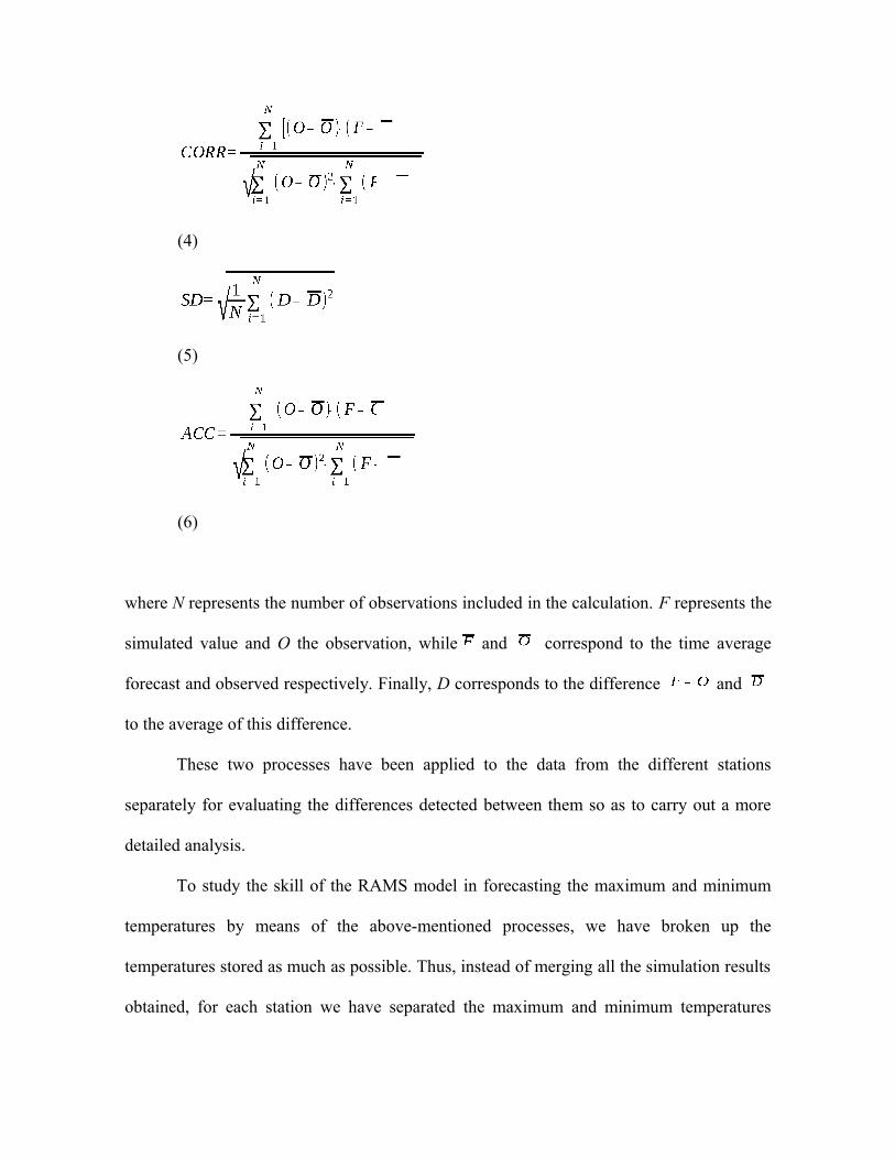
(4)

(5)

(6)

where N represents the number of observations included in the calculation. F represents the

simulated value and O the observation, while and correspond to the time average

forecast and observed respectively. Finally, D corresponds to the difference and

to the average of this difference.

These two processes have been applied to the data from the different stations

separately for evaluating the differences detected between them so as to carry out a more

detailed analysis.

To study the skill of the RAMS model in forecasting the maximum and minimum

temperatures by means of the above-mentioned processes, we have broken up the

temperatures stored as much as possible. Thus, instead of merging all the simulation results

obtained, for each station we have separated the maximum and minimum temperatures

forecasted by RAMS within each forecast day and each forecast cycle. With the

computational resources used to carry out this study, a high-resolution simulation takes

about 6 hours to finish. And even if the available computational resources permitted the

simulation time to be reduced, the restriction in the availability of data to initialize the

model would still delay the forecast release. It follows that, even if better computational

resources are available, the configuration of the model can always be improved, i.e., by

increasing the horizontal resolution, number of points, etc. In this case, again, more

resources are needed to finish the simulation on time. Thus, we decided to implement two

daily RAMS runs: a first forecast that can provide an early warning of temperature spikes,

and an update forecast that follows the evolution of the situation with recent data. To

analyse the skill of the model in both forecast releases and to assure that the GFS forecast

cycle does not significantly affect the RAMS results, 00 UTC and 12 UTC RAMS forecast

cycles are analysed separately. This will show if the RAMS initialization method used is

reasonably applicable. In relation to the forecast day, our aim is to study the stability of the

model and the quality of the forecast results for the three simulation days. Thus, we will

analyse how far in advance RAMS is able to forecast the observed maximum and minimum

temperatures. RAMS model has been run from 1 June to 31 August for the 2007, 2008,

2009 and 2010 summer season. We have analysed the behaviour of the model in the two

daily cycles and the three simulation days of these four years. To clarify the analysis of

results, we only present those obtained merging all summer periods. However, it has been

observed that the results are very similar evaluating each year separately (not shown),

reflecting the model patterns in forecasting maximum and minimum temperatures within

the summer season. Finally, in the next section we present both the results found for both

the 00 and 12 UTC RAMS forecast cycles. The first is the one basically used to elaborate

the high temperature hazard maps and activate the protocols established by the General

Direction of Public Health of the Regional Government of Valencia. Nevertheless, results

for the 12 UTC RAMS forecast cycle are also presented to show that both forecast cycles

yield very similar results.

Additionally, in order to investigate the representative errors of the surface stations,

we have used the procedure suggested by Myrick and Horel (2006) and Federico (2011).

This method is based on the observation ( ) and background ( ) error covariances,

where the background field is the RAMS first-day forecast for the 0000 UTC simulation,

computed as previously described. The covariance between observational innovations

(difference between observation and background values) at two points is computed as a

function of the distance r from all background field-observation pairs during all summer

seasons:

(7)

where o is the measurement and b is the background field interpolated at the station point.

If we assume that: (a) the observational errors are uncorrelated with one another; and (b)

the background and the observational errors are uncorrelated, Eq. (7) becomes:

(8)

and

(9)

where ρ(r) is the background error correlation, which is assumed as an isotropic function of

the distance.

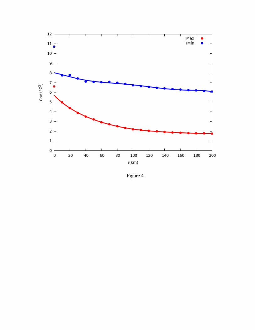
We have represented the covariance of observational innovations as a function of

distance r for all summer seasons and for maximum and minimum temperatures (Fig. 4). It

is observed that the maximum temperature covariance drops sharply as a function of

horizontal distance and remains almost constant for greater distances. However, a rather

smoother covariance rate is found for the minimum temperature. For this parameter, a low

variation is produced compared to that detected for the maximum. None of this curves

asymptotes to 0, which suggests that the RAMS background fields exhibit errors that

remain correlated over distances of hundreds of kilometers, particularly in the case of the

minimum temperatures. Fitting a least squares curve to the innovation covariance values for

horizontal distances greater than 10 km and extrapolating the curve back to r = 0 makes it

possible to estimate the ( ). A 6th-order polynomial has been chosen to fit the covariance

values at r = 0, because it minimizes the of the interpolating polynomial (Federico,

2011). As a result, for the maximum (minimum) temperature is estimated to be equal to

5.70 ºC2 (8.02 ºC2). Using Eq. 8, the observation error covariance can then be estimated

from the difference between the innovation covariance value at distance zero and the

estimate of . Thus, for maximum (minimum) temperature is estimated to be equal

to 0.90 ºC2 (2.68 ºC2). Based on these results, we may see that is quite reduced in

relation to . However, a significant difference is identified in the observational

representative error between the two parameters analysed, with the minimum temperatures

presenting the largest values. In this case, the innovation covariance does not display a

relevant decrease at long distance when compared to the maximum, showing the influence

of the RAMS forecast far from the corresponding station and reducing the

representativeness of the minimum temperatures. As a result, it appears that this condition

is likely to play a significant role in the overestimation of the RAMS errors for this

parameter over complex orography, as shown in the next section.

4. Results.

Because of the topographic, climatic and physical diversity of the study area, we

have carried out a detailed analysis based on separating the data available from the different

CEAM and IVIA stations. This has allowed us to differentiate the coastal stations from the

inland ones and see how the topography and other physical characteristics of the station

location can affect the observation and how the model is able to capture these effects. Thus,

we were interested in finding out if the model might follow a pattern that could be isolated.

There are basically two ways to do this. The first is to merge the two types of data and

study the results obtained with all the data from each type separately (Pérez-Landa et al.,

2007). This permits working with two groups of data, and relating the results to all the data

connected to a concrete type. The second way to carry out the study is to select some

stations from the different areas and analyse each of them separately (Palau et al., 2005).

The latter could show the skill of the model not only to reproduce the characteristics of the

station location but also to detect relationships between different stations in different

locations but with similar physical or climatic characteristics. We have adopted the second

formula. In a previous step, the CEAM and IVIA scatter plots and statistics were calculated

for the different meteorological magnitudes and all the stations within the study area. This

permitted us to carry out a preliminary analysis of the different stations. Then we grouped

each station according to similar physical and climatic characteristics (Miró et al., 2006)

and evaluated them individually based on the scatter plots and statistical scores. This initial

analysis showed that RAMS presents a clearly different behaviour for coastal stations than

for inland stations when forecasting maximum and minimum temperatures. Moreover, pre-

coastal stations behave like either coastal or inland stations according to topographic and

physical issues. As a result of this finding, some representative stations within the study

area have been selected to analyse and discuss the RAMS results in the current section (Fig.

5).

As we can see, for coastal stations (Fig. 6a, 6c, 6e), RAMS generally does a good

job of reproducing the temperature cycle and magnitude for the whole period in the

maximum as well as the minimum temperatures. It also captures quite well the observed

maximum and minimum temperature peaks. However, with respect to the deviations

between the modeled and measured maximum and minimum temperatures a different

behaviour is observed. In the case of the maximum temperature, the model forecast has a

clear tendency to underpredict the observations. On the other hand, the deviations in the

minimum temperature forecasted by the model have a tendency to overpredict the

observations. On coastal locations, the model seems to behave better for minimum

temperatures than for maximum temperatures, as reflected in the better fit between

simulated values and observed values. In forecasting both variables, RAMS shows very

stable behaviour, as can be appreciated in the similar results obtained for the three days of

simulation. In fact, for some stations and situations, RAMS provides better forecasts for the

second and third day than for the first one (Fig. 6a, 6c, 6e).

RAMS-simulated maximum temperatures for inland stations agree quite well with

the observed maximum, better than for coastal stations (Fig. 6b, 6d, 6f). In this case, the

separation between forecast and measurement data is substantially reduced compared with

that observed for coastal stations. Besides, these differences have a tendency to overpredict

the measurement, thus reversing the tendency obtained for coastal stations. In the case of

minimum temperatures for inland stations, the skill of the model decreases in general with

respect to their forecast for coastal stations. For inland stations, the model tends to

overpredict the minimum temperature forecast, as was also observed for coastal stations.

Comparing both kinds of stations, the differences between forecasted and measured

minimum temperatures for inland stations are greater than those obtained for coastal

stations. This behaviour of the model is maintained for the three days of simulation (Fig.

6b, 6d, 6f).

Finally, as can be seen in Fig. 7, the results obtained for the 12 UTC RAMS cycle

are very similar to those released by the 00 UTC RAMS cycle.

To obtain more specific information on the global skill of the RAMS model for

determining maximum and minimum temperatures within the Valencia Region, we have

used different statistical indexes to carry out a quantitative analysis for each individual

station in the CEAM and IVIA measurement networks. Tables 2 and 3 show the statistics

for the maximum and minimum temperatures obtained for the representative coastal, pre-

coastal and inland stations, on the first day of simulation for all forecasting period (summer

2007, 2008, 2009 and 2010).

Analysing the stations not far from the coast (pre-coastal) we have found that the

behaviour of the model with respect to both maximum and minimum temperatures for these

locations is generally related to the topographic complexity of the station location. Table 2

presents the maximum temperature statistics obtained for the stations selected. The RMSE

values are an indication of how well the RAMS model is able to simulate this variable. In

general, the values obtained are near 2 ºC. Similar results are found for the SD score, with

the lowest ones corresponding to inland stations, as in the case of CAS station with a value

of 1.58 ºC. For coastal stations, the model has a low negative bias (below 2 ºC), with

average values also showing an underestimation for all the coastal stations. In this case, the

RAMS-simulated heating is lower than the observed heating. Besides, the ACC values,

above 0.60, indicate the usefulness of the model for the maximum temperature at the coast.

For the inland station and the pre-coastal ones, the model has a slight positive bias, showing

that RAMS is capturing very well the heating effects on the daytime temperature for these

locations. Furthermore, the high ACC values, above 0.80, indicate that the model is able to

capture very well the day-to-day variability for the maximum temperature inland. This

statistical score also indicates the model skill for pre-coastal stations, with values closer to

those observed at the coast or inland, depending on the station location. All the IoA values

are near 0.9, indicating that the daily and the day-to-day maximum temperature evolution is

very well reproduced by the model. Moreover, CORR score has values near 0.9, showing a

very good relation between model-data maximum temperatures.

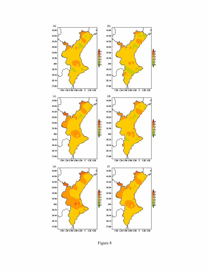
To procure a more detailed picture, maps of the bias and RMSE statistic scores has

been drawn for maximum and minimum temperatures within the Valencia Region, using

the available CEAM and IVIA data (34 stations operated by CEAM and 43 operated by

IVIA; Fig. 1). The map for RMSE corresponding to the maximum temperatures is

introduced in Fig. 8. In general, the RMSE for the whole territory remains around 2 ºC,

with the exception of some areas. This can be due to the complexity of the area surrounding

the station that produces the model not to capture the local characteristics properly.

Besides, although the values for the three forecast days are close to the ones obtained for

the first day, the RMSE shows a small increase with the forecasting time. In this sense, the

area spanned for RMSE values higher than 2 ºC within the third day of simulation is more

extensive than that observed in the first day. These results are also reproduced in the 12

UTC RAMS cycle (Fig. 8b, 8d, 8f), with slightly better values of RMSE than the estimated

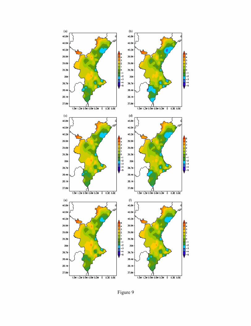
within the 00 UTC cycle. In the case of the bias, we can see that the values for this score

show an underestimation of the observations for coastal stations while an overestimation is

reproduced by the model for maximum temperatures as we move inland (Fig. 9). There is a

bias distribution associated with the complex terrain as well as with steep topography,

which is a tendency reproduced by RAMS for the entire region of study.

Table 3 shows the statistics on minimum temperatures obtained merging data for all

years. In this case, RMSE values obtained for the coastal and the pre-coastal stations

located over areas of low topographical complexity are near 2 ºC. The values obtained for

the inland and more inland pre-coastal stations (LLI), reveal a systematic error of the

model, with values higher than 4 ºC. For the SD, the lowest scores are reached over flatter

terrain, with values lower than 2 ºC. This error can also be seen for the bias and average

scores, which show a clear overestimation for nearly all stations. For inland as well as pre-

coastal stations located in areas of high topographical complexity, bias values are near 3 ºC.

In contrast, for all coastal stations and the pre-coastal stations located in a flatter terrain, the

bias scores show values near or even lower than 1 ºC. The IoA for the minimum

temperature is near 0.8 for the coastal stations. For inland stations, the IoA values are near

0.6. Thus, although the model reproduces the daily and day-to-day minimum temperature

evolution quite well for coastal stations, it has more problems in this respect for inland

stations. This result is also shown in the CORR score. Once again, for pre-coastal stations,

the behaviour of the IoA and CORR statistics is similar to that described for the bias and

RMSE scores. These results are also shown by the ACC score. In this case, the model is

still able to capture the day-to-day variability for the minimum temperature at the coast, as

indicated by the values of ACC, near 0.70. However, this score shows the complexity in

forecasting minimum temperatures inland. In this regard, the ACC value falls below 0.60.

The results shown in tables 2 and 3 for the 00 UTC forecast are very similar to those

obtained for the 12 UTC RAMS forecast update (not shown).

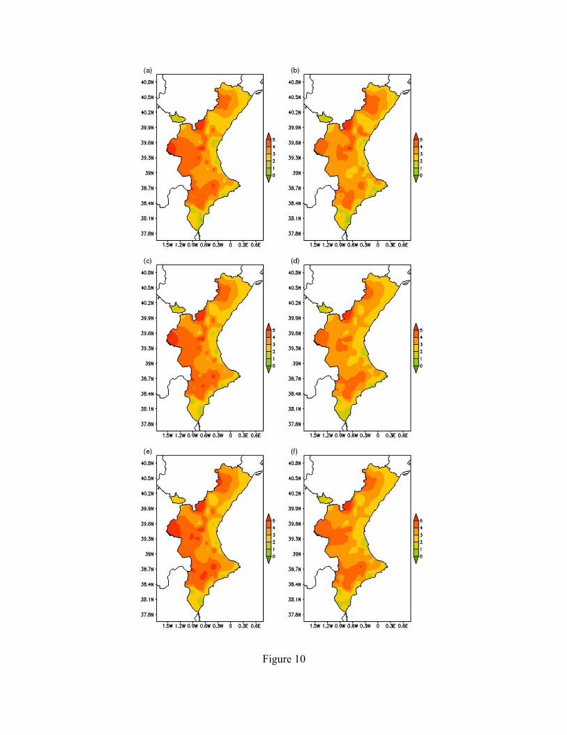
The RMSE for minimum temperatures increases slightly as we move forward in the

simulation, although the values are close to the ones obtained for the first day of simulation

(Fig. 10). This result is reproduced both by the 00 and 12 UTC RAMS cycles. However, it

seems that using the 12 UTC simulations, RAMS produces slightly lower values of RMSE

compared to those obtained using the 00 UTC cycle. As a difference with maximum

temperatures, when modeling the minimum, higher errors are obtained. In this case, areas

with RMSE score higher than 3 ºC are more extensive than those estimated for the

maximum temperatures. According to the bias results, significant differences between both

daily temperatures are also reproduced by the model (Fig. 11). As a result, for minimum

temperatures, the bias has a general tendency to overestimate the measured values with

different degree of accuracy. Thus, reduced areas of negative bias are observed.

Furthermore, the values of this statistics for the minimum are higher than those estimated

for the maximum temperatures both in magnitude as well as regarding spatial area

distribution. This effect of bias is reproduced for the complete Valencia Region, especially

in those areas where the terrain complexity is evident.

In Estrela et al. (2008), it is explained the high-temperature prediction system for

the Valencia Region based on the RAMS-forecast maximum and minimum temperatures. A

different degree of agreement is found between the forecast and observed hazard-level for

coastal and inland areas, higher in the coast. The current work explains these results due to

the fact that the minimum temperatures are over-predicted by RAMS inland. This provokes

a clear tendency to forecast higher hazard-levels over these areas compared to those

observed. In contrast, when the maximum temperature plays the most significant role in

determining the high-temperature hazard-level, the system is rather useful as little

differences are found between the forecast and observed hazard-level. These results seem

clear looking at Fig. 6 and Fig. 7. In this sense, it is also observed that for coastal stations,

the distribution of both the maximum and minimum temperatures shows a skilled degree of

correlation between the forecast and observed hazard-levels.

5. Conclusions.

The main aim of this work has been to evaluate the skill of the RAMS model in

forecasting summertime maximum and minimum temperatures for the whole Valencia

Region, to be used within the extreme-temperature forecast and warning system

implemented in this area. For this, we have used the high-resolution configuration of

RAMS running operationally at CEAM. We have focused on an evaluation of the model,

using all the data available for the 2007, 2008, 2009 and 2010 summer periods from both

inland and coastal stations. The results indicate that RAMS reproduces the maximum

temperature cycles quite well and is also able to capture the high maximum temperature

peaks that occurred in the summer season. In addition, the model can also capture the

minimum temperature peaks produced in this period. However, RAMS has more

difficulties in determining the minimum temperature, tending to overestimate the

observations. Regarding the different station locations, we have found that RAMS

behaviour with respect to both maximum and minimum temperatures differs between

inland stations and coastal stations. In relation to the maximum, RAMS shows good

agreement with the observations at both types of stations. However, the behaviour of the

model is not the same as the tendency of the model. In this sense, RAMS tends to over-

predict the observations at inland stations while underestimating the coastal ones. On the

other hand, the forecasted minimum temperatures have a general tendency to over-predict

the measurements at both kinds of stations. Although the model results for coastal locations

agree quite well with the observations, higher errors are encountered for the most inland

locations, where the topographical complexity is more marked. In relation to the minimum

temperatures forecasted by the model for pre-coastal stations, RAMS follows the behaviour

shown for the coastal stations or the inland stations depending on the topographical

complexity of the measurement site.

The same results are found for the three days of simulation, indicating that RAMS

maximum and minimum temperature forecasts are very stable for at least three forecast

days. Moreover, the initialization method used for RAMS is valid as the results obtained

are very similar in both daily simulation cycles. The influence of the temporal gap in the

GFS data used to initiate the RAMS model in the operational implementation of this study

is not critical in the results obtained. Thus, RAMS provides very useful information at least

three days in advance and the daily update forecast basically follows the first daily forecast

behaviour.

Accordingly, RAMS is able to reproduce maximum temperatures with a great de-

gree of accuracy and thus could be perfectly applied to forecast maximum temperatures for

the whole Valencia Region. Besides, RAMS is very useful for minimum temperature fore-

casting at coastal stations within the Valencia Region and it is also able to reproduce the

minimum temperature peaks quite well over the whole Valencia Region. On the contrary,

RAMS significantly overestimates the minimum temperature for inland areas for a consid-

erable number of days within the summer period. This issue is probably related to the noc-

turnal cooling of the ground which is not satisfactorily simulated by the model, as has

already been pointed out in diagnostic studies (Palau et al., 2005; Pérez-Landa et al., 2007).

The same results have also been found for other Mediterranean Regions using other real-

time mesoscale models (Bartzokas et al., 2010). Likewise, in other areas with Mediter-

ranean-type climate regimes, it has been found that atmospheric humidity is the main cause

of elevated minimum temperatures (Gershunov et al., 2009; Gershunov and Guirguis,

2012). Finally, the larger representativeness error for the minimum temperature using the

current methodology could also be related to the overestimation of this parameter in com-

plex orography.

It is the plan of the authors to continue verifying the CEAM RAMS real-time

forecasting system by focusing on the skill of the model in forecasting other meteorological

variables within the Valencia Region. More in-depth analysis will help to isolate the

processes causing the main differences between RAMS-forecasted and observed maximum

and minimum temperatures, with the aim of improving the system implemented.

Acknowledgement. This work has been funded by the Spanish Ministerio de Educación y

Ciencia through the projects CGL2008-04550 (Proyecto NIEVA), CSD2007-00067

CONSOLIDER-INGENIO 2010 (Proyecto GRACCIE) and CGL2007-65774/CLI

(Proyecto MAPSAT), and by the Regional Government of Valencia through the contract

“Simulación de las olas de calor e invasiones de frío y su regionalización en la Comunitat

Valenciana” (“Heat wave and cold invasion simulation and their regionalization at the

Valencia Region”) and the project PROMETEO/2009/086. The authors wish to thank F.

Pastor, J. Miró and M. J. Barberà for their appreciable collaboration as well as J. L. Palau

and R. Niclòs for their constructive comments while writing this paper. We also want to

thank Jackie Scheiding for the review of the English text. NCEP are acknowledged for

providing the GFS meteorological forecasts for RAMS initialization.

References

Bartzokas A, Kotroni V, Lagouvardos K, Lolis CJ, Gkikas A, Tsirogianni MI (2010).

Weather forecast in north-western greece: Riskmed warnings and verification of mm5

model. Natural Hazards and Earth System Sciences 10:383-394.

Case JL Manobianco J, Dianic AV, Wheeler MM, Harms DE, Parks CR (2002). Verifica-

tion of high-resolution rams forecasts over east-central Florida during the 1999 and 2000

summer months. Weather and Forecasting 17:1133-1151.

Chen C, Cotton WR (1983). A one-dimensional simulation of the stratocumulus-capped

mixed layer. Boundary-Layer Meteorology 25:289-321.

Cotton WR, Pielke RAS, Walko RL, Liston GE, Tremback CJ, Jiang H, McAnelly RL,

Harrington JY, Nicholls ME, Carrio GG, McFadden JP (2003). RAMS 2001: Current status

and future directions. Meteorology and Atmospheric Physics 82 (1-4):5-29.

Corell-Custardoy D, Valiente-Pardo JA, Estrela-Navarro MJ, García-Sánchez F, Azorín-

Molina C (2010). Red de torres meteorológicas de la Fundación CEAM (CEAM

meteorological station network), in: 2nd Meeting on Meteorology and Climatology of the

Western Mediterranean, Valencia, Spain.

Dudhia J (1993). A non-hydrostatic version of the Penn State/NCAR mesoscale model: val-

idation tests and simulation of an Atlantic cyclone and cold front, Mon. Weather Rev., 121,

1493–1513.

Estrela M, Pastor F, Miró J, Gómez I, Barberà M (2007). Heat waves prediction system in a

mediterranean area (valencia region). 7th EMS Annual Meeting / 8th European Conference

on Applications of Meteorology.

Estrela M, Pastor F, Miró J, Gómez I, Barberà M (2008): Diseño de un sistema de predic-

ción de niveles de riesgo por temperaturas extremas para la Comunidad Valenciana. Olas

de calor, 235-252. Riesgos Climáticos y Cambio Global, Colección Interciencias.

Fast JD (1995). Mesoscale modeling in areas of highly complex terrain employing a four-

dimensional data assimilation technique. Journal of Applied Meteorology 34:2762-2782.

Federico S (2011). Verification of surface minimum, mean, and maximum temperature

forecasts in Calabria for summer 2008. Natural Hazards and Earth System Sciences 11:

487-500.

Gershunov A, Cayan D, Iacobellis S (2009). The great 2006 heat wave over California and

Nevada: Signal of an increasing trend. Journal of Climate 22: 6181-6203.

Gershunov A, Guirguis K (2012). California heat waves in the present and future.

Geophysical Research Letters 39, L18710, doi:10.1029/2012GL052979.

Gómez I, Pastor F, Estrela MJ, Miró J, Barberà MJ (2007). Development of a Java-based

graphical user interface to control/monitor a real-time forecast and alert system. 7th EMS

Annual Meeting/ 8th European Conference on Applications of Meteorology, San Lorenzo

de El Escorial, Spain.

Gómez I, Estrela M (2009a). Operational forecasting of daily temperatures in the valencia

region. Part I: maximum temperatures in summer. 9th EMS Annual Meeting/9th European

Conference on Applications of Meteorology, Toulouse, France.

Gómez I , Estrela M (2009b). Operational forecasting of daily temperatures in the valencia

region. Part II: minimum temperatures in winter. 9th EMS Annual Meeting/9th European

Conference on Applications of Meteorology, Toulouse, France.

Gómez I, Estrela MJ (2010). Design and development of a java-based graphical user inter-

face to monitor/control a meteorological real-time forecasting system. Computers &

Geosciences 36:1345-1354. doi:10.1016/j.cageo.2010.05.005.

Gómez I, Pastor F, Estrela MJ (2011). Sensitivity of a mesoscale model to different

convective parameterization schemes in a heavy rain event. Natural Hazards and Earth

System Sciences 11: 343-357, doi: 10.5194/nhess-11-343-2011.

Gómez I, Marin MJ, Pastor F, Estrela MJ (2012). Improvement of the Valencia region ul-

travioleta index (UVI) forecasting system. Computers & Geosciences 41: 72-82, doi:

10.1016/j.cageo.2011.08.015.

Gómez-Tejedor JA, Estrela MJ, Millán MM (1999). A mesoscale model application to fire

weather winds. International Journal of Wildland Fire 9:255-263.

IVIA (2003): IVIA (instituto valenciano de investigaciones agrarias): Servicio de tecnolo-

gía del riego. SIAR (servicio integral de asesoramiento al regante) red de estaciones agro-

climáticas de la Comunitat Valenciana. Tech. rep. URL http://estaciones.ivia.es/estacion.

Mellor G, Yamada T (1982). Development of a turbulence closure model for geophysical

fluid problems. Reviews of Geophysics and Space Physics 20:851-875.

Miró JJ, Estrela MJ, Millán MM (2006). Summer temperature trends in a mediterranean

area (valencia region). International Journal of Climatology 26:1051-1073.

Molinari J. (1985). A general form of kuo's cumulus parameterization. Monthly Weather

Review 113:1411-1416.

Myrick DT, Horel JH (2006). Verification of surface temperature from the National

Digital Forecast Database over the western United States, Weather and Forecasting,

21:869-

892.

Palau JL, Pérez-Landa G, Diéguez JJ, Monter C, Millán MM (2005). The importance of

meteorological scales to forecast air pollution scenarios on coastal complex terrain. Atmo-

spheric Chemistry and Physics 5:2771-2785.

Pastor F, Estrela MJ, Peñarrocha D, Millán MM (2001). Torrential rains on the spanish

mediterranean coast. Modeling the effects of the sea surface temperature. Journal of Ap-

plied Meteorology 40(7):1180-1195.

Pastor F, Gómez I, Estrela MJ (2010). Numerical study of the october 2007 flash flood in

the Valencia region (Eastern Spain): the role of orography. Natural Hazards and Earth Sys-

tem Sciences 10:1331-1345. doi:10.5194/nhess-10-1331-2010.

Pérez-Landa G, Ciais P, Sanz MJ, Gioli B, Miglietta F, Palau JL, Gangoiti G, Millán M

(2007). Mesoscale circulations over complex terrain in the Valencia coastal region, Spain.

Part 1: Simulation of diurnal circulation regimes. Atmospheric Chemistry and Physics

7:1835-1849.

Pielke Sr. RA (2002). Mesoscale meteorological modeling. 2nd Edition. Academic Press,

San Diego, CA, 676 pp.

Salvador R, Calbó J, Millán M (1999). Horizontal grid size selection and its influence

on mesoscale model simulations. Journal of Applied Meteorology 39(9):1311-1329.

Salvador R, Millán M, Mantilla E, Baldasano JM. 1997. Mesoscale modelling of atmo-

spheric processes over the western mediterranean area during summer. International

Journal of Environment and Pollution 8:513-529.

Tremback CJ, Walko RL, Bell MJ (2002). RAMS/HYPACT Evaluation and Visualization

Utilities (REVU) user´s guide, version 2.3.1, Technical Report.

Walko RL, Cotton WR, Meyers MP, Harrington JY (1995). New RAMS cloud microphys-

ics parameterization. Part I: The single-moment scheme. Atmospheric Research 38:29-62.

Walko RL, Band LE, Baron J, Kittel TGF, Lammers R, Lee TJ, Ojima D, Pielke RA,

Taylor C, Tague C, Tremback CJ, Vidale PL (2000). Coupled atmospheric-biophysics-hy-

drology models for environmental modeling. Journal of Applied Meteorology 39:931-944.

Willmott CJ (1981). On the validation of models. Physical Geography 2 (2):184-194.

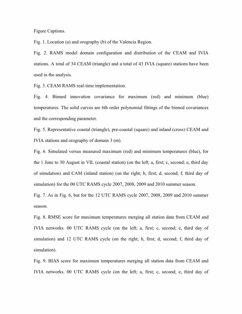
Figure Captions.

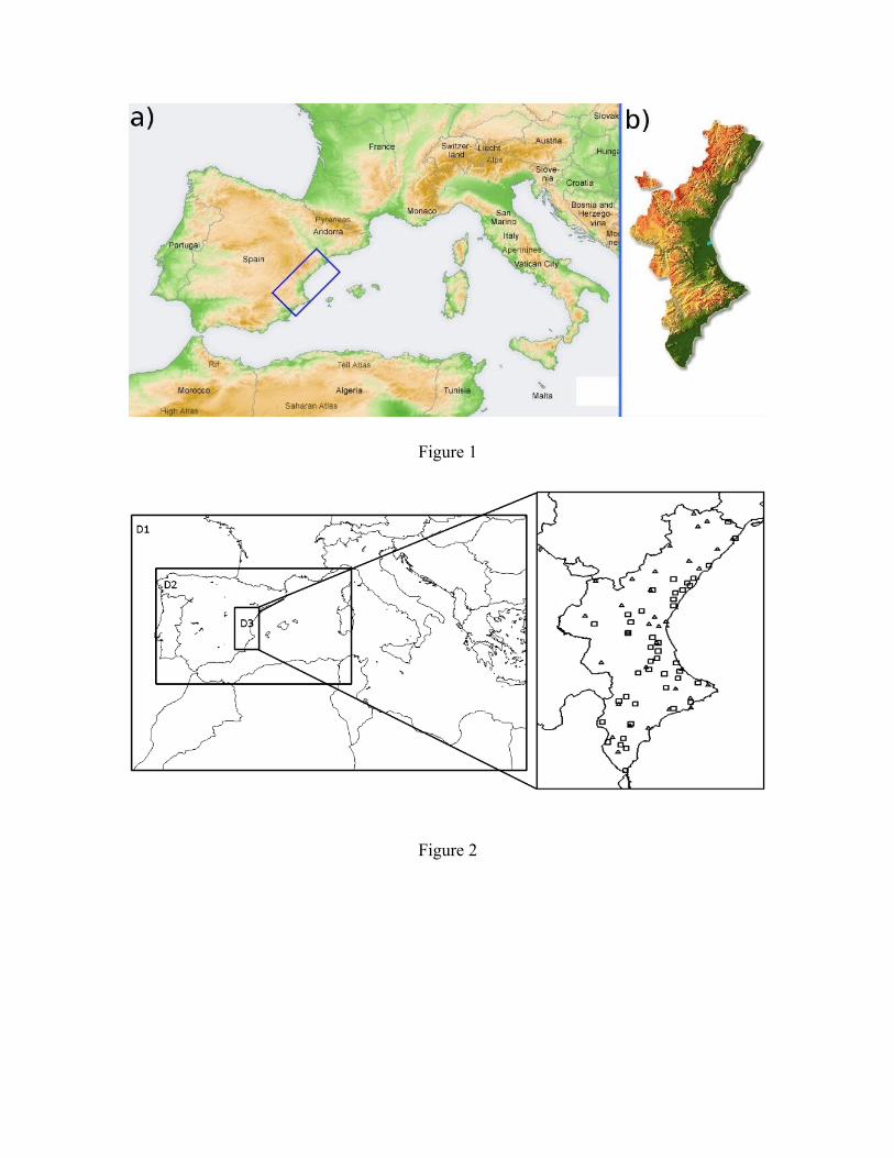
Fig. 1. Location (a) and orography (b) of the Valencia Region.

Fig. 2. RAMS model domain configuration and distribution of the CEAM and IVIA

stations. A total of 34 CEAM (triangle) and a total of 43 IVIA (square) stations have been

used in the analysis.

Fig. 3. CEAM RAMS real-time implementation.

Fig. 4. Binned innovation covariance for maximum (red) and minimum (blue)

temperatures. The solid curves are 6th order polynomial fittings of the binned covariances

and the corresponding parameter.

Fig. 5. Representative coastal (triangle), pre-coastal (square) and inland (cross) CEAM and

IVIA stations and orography of domain 3 (m).

Fig. 6. Simulated versus measured maximum (red) and minimum temperatures (blue), for

the 1 June to 30 August in VIL (coastal station) (on the left; a, first; c, second; e, third day

of simulation) and CAM (inland station) (on the right; b, first; d, second; f, third day of

simulation) for the 00 UTC RAMS cycle 2007, 2008, 2009 and 2010 summer season.

Fig. 7. As in Fig. 6, but for the 12 UTC RAMS cycle 2007, 2008, 2009 and 2010 summer

season.

Fig. 8. RMSE score for maximum temperatures merging all station data from CEAM and

IVIA networks. 00 UTC RAMS cycle (on the left; a, first; c, second; e, third day of

simulation) and 12 UTC RAMS cycle (on the right; b, first; d, second; f, third day of

simulation).

Fig. 9. BIAS score for maximum temperatures merging all station data from CEAM and

IVIA networks. 00 UTC RAMS cycle (on the left; a, first; c, second; e, third day of

simulation) and 12 UTC RAMS cycle (on the right; b, first; d, second; f, third day of

simulation).

Fig 10. As in Fig. 8, but for minimum temperatures.

Fig 11. As in Fig. 9, but for minimum temperatures.

Tables.

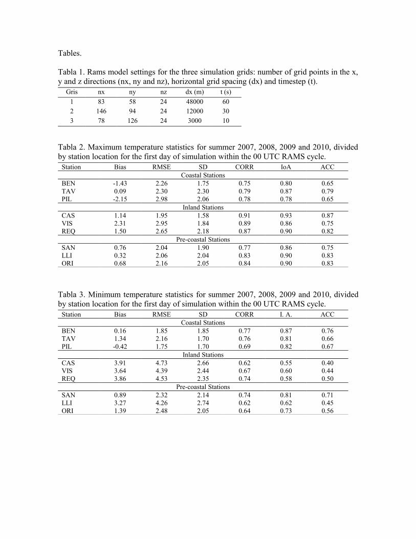
Tabla 1. Rams model settings for the three simulation grids: number of grid points in the x,y and z directions (nx, ny and nz), horizontal grid spacing (dx) and timestep (t).

Gris nx ny nz dx (m) t (s)

1 83 58 24 48000 60

2 146 94 24 12000 30

3 78 126 24 3000 10

Tabla 2. Maximum temperature statistics for summer 2007, 2008, 2009 and 2010, dividedby station location for the first day of simulation within the 00 UTC RAMS cycle.

Station Bias RMSE SD CORR IoA ACCCoastal Stations

BEN -1.43 2.26 1.75 0.75 0.80 0.65TAV 0.09 2.30 2.30 0.79 0.87 0.79PIL -2.15 2.98 2.06 0.78 0.78 0.65

Inland StationsCAS 1.14 1.95 1.58 0.91 0.93 0.87VIS 2.31 2.95 1.84 0.89 0.86 0.75REQ 1.50 2.65 2.18 0.87 0.90 0.82

Pre-coastal StationsSAN 0.76 2.04 1.90 0.77 0.86 0.75LLI 0.32 2.06 2.04 0.83 0.90 0.83ORI 0.68 2.16 2.05 0.84 0.90 0.83

Tabla 3. Minimum temperature statistics for summer 2007, 2008, 2009 and 2010, dividedby station location for the first day of simulation within the 00 UTC RAMS cycle.

Station Bias RMSE SD CORR I. A. ACCCoastal Stations

BEN 0.16 1.85 1.85 0.77 0.87 0.76TAV 1.34 2.16 1.70 0.76 0.81 0.66PIL -0.42 1.75 1.70 0.69 0.82 0.67

Inland StationsCAS 3.91 4.73 2.66 0.62 0.55 0.40VIS 3.64 4.39 2.44 0.67 0.60 0.44REQ 3.86 4.53 2.35 0.74 0.58 0.50

Pre-coastal StationsSAN 0.89 2.32 2.14 0.74 0.81 0.71LLI 3.27 4.26 2.74 0.62 0.62 0.45ORI 1.39 2.48 2.05 0.64 0.73 0.56

Figure 1

Figure 2

Figure 3

Figure 4

Figure 5

Figure 6

Figure 7

Figure 8

Figure 9

Figure 10

Figure 11